the Creative Commons Attribution 4.0 License.
the Creative Commons Attribution 4.0 License.
 | 23 Aug 2022
A dynamic hierarchical Bayesian approach for forecasting vegetation condition
Peter D. Hurley
James M. Muthoka
Andrew Bowell
Seb Oliver
Pedram Rowhani
Agricultural drought, which occurs due to a significant reduction in the moisture required for vegetation growth, is the most complex amongst all drought categories. The onset of agriculture drought is slow and can occur over vast areas with varying spatial effects, differing in areas with a particular vegetation land cover or specific agro-ecological sub-regions. These spatial variations imply that monitoring and forecasting agricultural drought require complex models that consider the spatial variations in a given region of interest. Hierarchical Bayesian models are suited for modelling such complex systems. Using partially pooled data with sub-groups that characterise spatial differences, these models can capture the sub-group variation while allowing flexibility and information sharing between these sub-groups. This paper's objective is to improve the accuracy and precision of agricultural drought forecasting in spatially diverse regions with a hierarchical Bayesian model. Results showed that the hierarchical Bayesian model was better at capturing the variability for the different agro-ecological zones and vegetation land covers compared to a regular Bayesian auto-regression distributed lags model. The forecasted vegetation condition and associated drought probabilities were more accurate and precise with the hierarchical Bayesian model at 4- to 10-week lead times. Forecasts from the hierarchical model exhibited higher hit rates with a low probability of false alarms for drought events in semi-arid and arid zones. The hierarchical Bayesian model also showed good transferable forecast skills over counties not included in the training data.
- Article
(11293 KB) - Full-text XML
- Companion paper
- BibTeX
- EndNote


Drought is a naturally occurring phenomenon that affects the food security of approximately 55 million people annually and can severely impact a country's economy (Vatter, 2019; Deleersnyder, 2018; Nicolai-Shaw et al., 2017). Drought, in most cases, is associated with below-average precipitation and is referred to as meteorological drought. Prolonged meteorological drought events mainly lead to a significant reduction in the amount of soil moisture required for vegetation growth, thus resulting in an agricultural drought (Heim, 2002; Boken et al., 2005). Hence, agricultural drought events are considered a physical manifestation of meteorological drought (Boken et al., 2005).
Agricultural drought, which is the focus of this paper, is known to be very complex (Boken et al., 2005); this is because, aside from the soil moisture dynamics, the severity of agriculture drought events is further augmented by over-exploitation of vegetation through various human and wildlife activities like deforestation and overgrazing (Lal, 2012).
Its onset can be slow and can occur in vast areas with varying spatial impact (Boken et al., 2005). For instance, the impact of drought may differ within a given region depending on whether it is dominated by trees, grasslands, or croplands. In croplands especially, variation in drought occurrences may be also attributed to farming practices. Spatial differences in drought impact can also arise due to the varied agro-ecological sub-regions within an affected area. These differences indicate that early warning systems (EWSs) for agricultural drought will require very complex models.
Drought EWSs have been recognised by global initiatives like the United Nations Sustainable Development Goals (SDGs) for effective drought monitoring and hazard preparedness (IISD, 2018). As such, international agencies like the United Nations Development Programme (UNDP) and the United States Agency for International Development (USAID) (https://usaid.gov/, last access: 3 October 2021) mandated to monitor drought hazards have developed and deployed several EWSs. These systems assist drought management officials and people living in drought-prone communities to prepare for hazardous events (UN, 2018). The Famine Early Warning Systems Network (FEWS NET) (https://fews.net/, last access: 3 October 2021) is an example of such EWSs. The system, developed by the USAID, utilises household data together with agro-climatic indicators and vegetation health to monitor drought and its impact (FEWSNET, 2021). However, drought forecasting for anticipatory action via the FEWS NET platform is mainly based on expert judgement (Funk et al., 2019) rather than the use of advanced statistical methods or machine learning models.
Recent advances in computational power and processing hardware have enabled researchers to develop and deploy machine learning models (Bishop and Nasrabadi, 2006) such as support vector machines (Shao and Lunetta, 2012) and various neural network architectures (Da Silva et al., 2017). Machine learning models enable the construction of predictive or prescriptive models using advanced statistical methods to capture hidden patterns in data (Bishop and Nasrabadi, 2006). In the field of drought research, most of the data used within machine learning models come from satellite earth observation (EO) images. These datasets are available over long temporal periods, cover vast areas, and are easy to access. Therefore, they provide a cost-effective way of developing models for monitoring and forecasting drought events over vast regions. Examples of such EO datasets include precipitation, soil moisture levels, normalised difference vegetation index (NDVI), enhanced vegetation index (EVI), and vegetation condition index (VCI) (Kogan, 1995), all derived from remotely sensed EO data. Nay et al. (2018), for instance, used the gradient boosting machine (GBM) model to forecast EVI with lagged spectral bands from the Moderate Resolution Imaging Spectroradiometer (MODIS) EO data. Tian et al. (2019) worked on forecasting dryland vegetation condition using NDVI via an eco-hydrological model driven by surface water extent also derived from MODIS images. Others include Barrett et al. (2020) and Adede et al. (2019), who applied Gaussian processes and artificial neural networks, respectively, in their research to develop robust models for short- to medium-term forecasts of vegetation conditions. All the models used in the cited works were mainly implemented by aggregating data over similar land cover types and agro-ecological zones (AEZs). The differences in the AEZs or land covers within the region were not considered.
This paper is part 2 of a previous study (Salakpi et al., 2022), where we used a Bayesian regression method to model the relationship between biophysical drivers and their effect on forecasting vegetation conditions. The approach was based on the classical “no-pooling” method (see Fig. 1), where we fitted separate regression models to data extracted from their respective regions. Pixels representing the biophysical indicators and vegetation conditions were sampled for different land cover and aggregated over the regions of interest. The modelling approach also treated the effects of climate and other biophysical factors on vegetation conditions independently for each region. The models were very skilful for medium- to long-term forecasts, but forecasts over regions with extensive cloud cover suffered due to the lack of data.

Figure 1Figure illustrating the concept of no pooling, complete pooling, and partial pooling of the data.
Although known to vary over the different regions, the effects of biophysical indicators on vegetation also show some similarities across the different regions (Vicente-Serrano, 2007). Data for such analysis can be pooled over all the regions of interest and analysed via the “complete-pooling” modelling approach to capture these similarities. This approach allows information sharing between the regions of interest, which is an advantage over the no-pooling approach (Gelman and Hill, 2006). However, the complete-pooling method is not very useful when the pooled data have sub-groupings, e.g. pooled soil moisture data from different regions with varied land cover types. In such a case, a more advanced approach would be to combine the strengths of both the no-pooling and complete-pooling methods into a model known as a “partial-pooled” model or “hierarchical model” (Gelman and Hill, 2006; Gelman et al., 2013). The hierarchical approach, which we demonstrate in this paper, enables flexibility between the sub-groups while treating them independently at the same time (Gelman and Hill, 2006). A hierarchical model, when implemented within a Bayesian framework, is referred to as a hierarchical Bayesian model (HBM) (Gelman et al., 2013). HBMs have in recent times been recognised as a powerful approach for modelling and analysing very complex data. They have been extensively used for research in fields like astrophysics, neuroscience, and genetics (Sánchez and Bernstein, 2019; George and Hawkins, 2005; Storz and Beaumont, 2002). Although not commonly used in the study of vegetation dynamics and drought monitoring, Senf et al. (2017) used an HBM to study the spatial and temporal variation in broad-leaved forests phenology using Landsat data.
The HBM is an extension of the regular Bayesian regression, where model parameters differ based on the variations within a given dataset (Gelman et al., 2013; Gelman and Hill, 2006). Thus, this paper seeks to test the concept of forecasting VCI, an EO-based agricultural drought indicator, with an HBM and answer the following question. Can we improve forecast accuracy and precision by separately learning parameters for the effects of lagged precipitation and soil moisture on vegetation conditions in each AEZ or over varied land cover types?.
Another advantage of using the HBM is its transferability (Senf et al., 2017). Transfer learning in this context refers to the process where models trained on a given dataset can be re-used to make predictions on different but related data that were not part of the training set (Z. Yang et al., 2017). The partially pooled data used in HBMs make them suitable for transfer learning primarily because the training data are pooled from multiple regions, and the sub-groupings within the data are the same for the non-training sample data (Rosenstein et al., 2005).
Our objectives for this proof of concept are to
-
improve the forecast accuracy and precision of the Bayesian auto-regression distributed lags (BARDL) model with a hierarchical Bayesian model in regions with diverse AEZs and land covers;
-
test the transfer learning property of hierarchical models that enables pre-trained models to be used on similar data from a different location without the need to retrain the model (Y. Yang et al., 2017).
2.1 Study area
To test our concept of forecasting vegetation condition with HBM, we sampled data from some selected counties in Kenya (Baringo, Kitui, Marsabit, Narok, Tana River, Turkana), shown in Fig. 2 with red boundary lines. The selected counties have diverse land use and land covers (LULCs), ranging from crops to evergreen forests. These counties also have varied AEZs, with rainfall and temperature patterns ranging from moderate to extreme. During the short and long rainfall seasons, annual mean precipitation ranges from 20 to 20 mm. Temperature across these counties also ranges from as low as 10 to 40 ∘C (Ayugi et al., 2016). The main economic activity in these counties is agriculture, predominantly agro-pastoral practices (Gebremeskel et al., 2019; Vatter, 2019). However, extreme climatic variations make this region prone to prolonged drought events, and the impact of these dry spells varies over the various land covers within the AEZs.
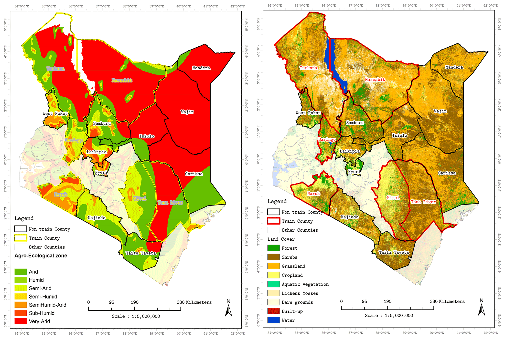
Figure 2Maps of Kenya showing agro-ecological zones (AEZs) and land cover maps for the counties from which pixels were sampled. Kenya AEZ boundary map credit: IGAD Climate Prediction and Application Centre (ICPAC). Land cover map credit: European Space Agency (ESA), Climate Change Initiative (CCI).
We selected only six counties because the algorithm used for parameter sampling by the HBM can be very time-consuming when the input data are more than 10 000 records. The sampling time is also mainly due to the complex nature of HBMs.
2.2 Data
2.2.1 Precipitation (rainfall estimates)
The precipitation data between 2001 and 2018 were obtained from the Climate Hazards Group InfraRed Precipitation (CHIRPS) project (Funk et al., 2015). The data comprise weather station data combined with rainfall estimates captured via satellite remote sensing. The dataset is available as daily 5km resolution images.
2.2.2 Soil moisture
The daily soil moisture products by the European Space Agency's Climate Change Initiative (ESA-CCI), from 2001 to 2018, were used for this work. The data represent soil moisture at a 10 cm soil depth and are derived from an algorithm that takes information from multiple active and passive synthetic aperture radar (SAR) satellites (Gruber et al., 2019; Dorigo et al., 2017; Y. Yang et al., 2017).
2.2.3 Surface reflectance
The vegetation index (VCI) used as a drought indicator for the work was derived from the bidirectional reflectance distribution function (BRDF)-corrected MODIS product, MCD43A4 Version 6 (Schaaf and Wang, 2015). The MCD43A4 products, available as daily 500 m resolution images, are captured in bands that range from visible to infrared. The VCI was derived from the NDVI, using the red and near-infrared (NIR) bands via Eq. (1).
After computing the NDVI, the VCI values are then computed using Eq. (2).
where NDVIi is the values for a given ith week, and NDVImin,i and NDVImax,i represent the long-term minimum and maximum NDVI values of a pixel for the ith week within a baseline year period.
2.3 Agro-ecological zones and vegetation land covers
Two HBMs were developed in this study, one based on AEZs and the other on land covers. AEZs are geographical areas characterised by similar climatic patterns and soil moisture levels suitable for agriculture and vegetation growth. These zones were created by the Food and Agriculture Organization (FAO) in collaboration with the International Institute for Applied Systems Analysis (IIASA) and are based on a framework that utilises a series of models with climate and land use information to quantify and map out the regions (Fischer et al., 2000). The zones are categorised as humid, semi-humid, arid, semi-arid, and very arid. These AEZs, from their definition, exhibit distinct climate properties; thus, a modelling approach that can separately learn parameters for the effects of precipitation and soil moisture on vegetation conditions based on the different AEZs can give a more accurate VCI forecast.
The AEZs in our study area can be seen in Table 1.
Table 1Table describing the agro-ecological zone, vegetation type, and annual rainfall levels.
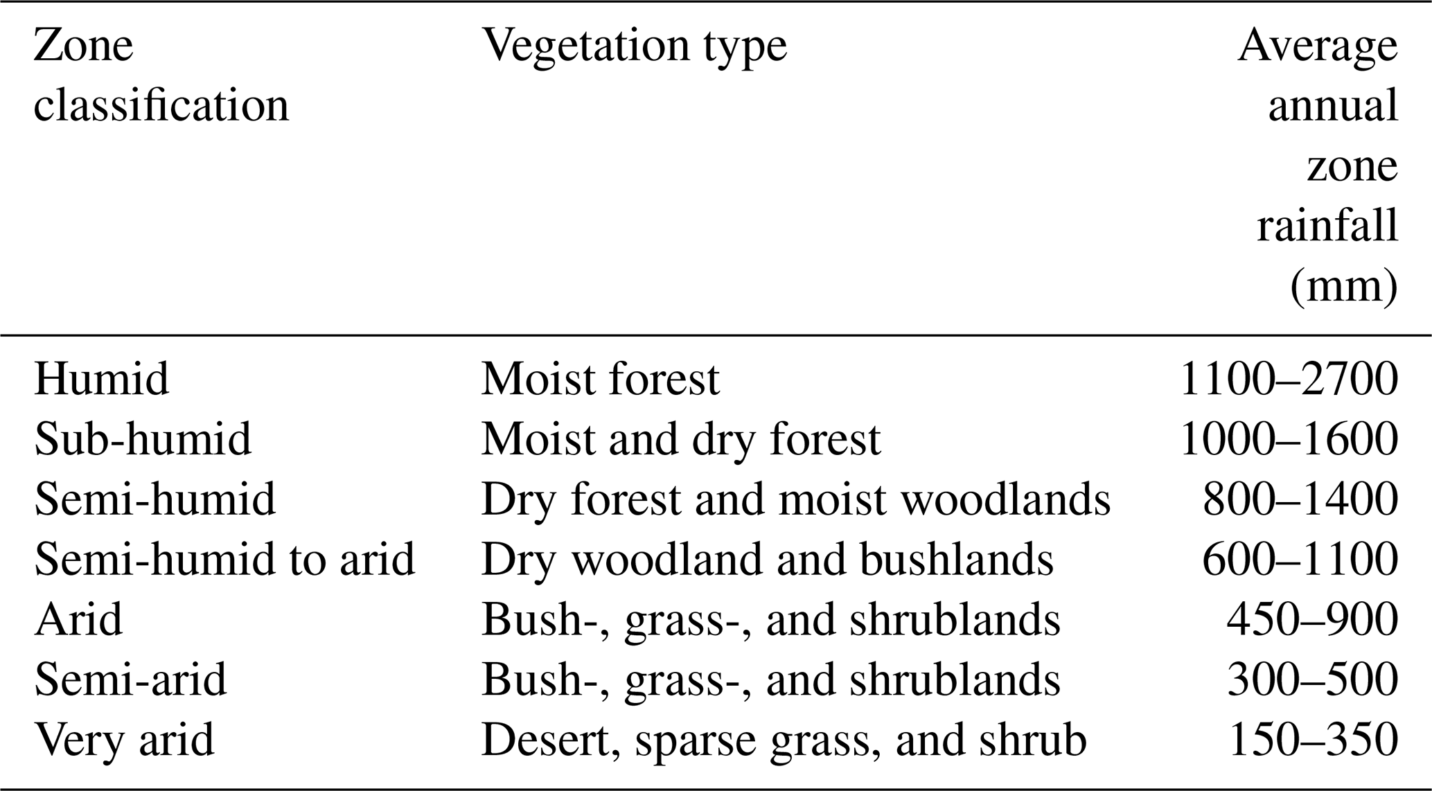
Source: Sombroek et al. (1982).
Most drought-prone regions are made of diverse vegetation covers; these include tree covers (forests), grasslands, shrubs, and croplands. The impact of drought on these land cover types varies both spatially and temporally. Thus, a drought forecast model should consider the varying effects of the biophysical factors on the various land covers. Using an HBM framework in this context enables us to achieve this. Data corresponding to the various vegetation land covers were extracted with the 2016 Sentinel 2 land use and land cover (LULC) map1.
3.1 Data pre-processing
A major challenge with using optical EO images is cloud cover and cloud shadows. In addition, pixel reflectance values sometimes fall outside the meaningful range due to errors during the atmospheric and radiometric correction process. These clouded and poor-quality pixels were filtered out with the quality assurance maps that come with the images. Weekly averages of VCI, precipitation, and soil moisture data corresponding to the vegetation land covers of interest were extracted from the selected counties using the European Space Agency (ESA) 2016 Sentinel 2 land use and land cover (LULC) map. The same data within the various AEZs were also extracted using the AEZ shapefiles produced by the IGAD Climate Prediction and Application Centre (ICPAC) (http://geoportal.icpac.net/layers/geonode%3Aken_aczones, last access: 3 October 2021). The temporal gaps, left by the removal of clouded pixels, were filled using the radial basis function (BBF) interpolation method, which ensures values obtained through interpolation over wide intervals do not go beyond the valid ranges (Rippa, 1999). The noise resulting from optical instrument failures and gap-filling processes was reduced with a penalised least-squares method (Whittaker smoother) (Eilers, 2003; Klisch and Atzberger, 2016). A 3-month (12 weeks) rolling average was applied to the VCI to make it VCI3M primarily because our stakeholders use it for their EWS. Applying the rolling averages enhanced the persistence in the VCI. Three-month precipitation (P3M) and soil moisture (SM3M) were also computed for consistency. Finally, to avoid the influence of strong seasonal cycles on the forecast values and make data stationary, the VCI3M, P3M, and SM3M data were converted to anomalies by subtracting the annual mean per land cover type and AEZ before fitting to the HBM. After forecasting, the subtracted seasonal means for the VCI3M (for each AEZ and land cover) were added back. All the variables were also standardised by subtracting the mean and dividing by the standard deviation to make the variable unitless and avoid the dominance of certain variables over others.
3.2 Forecast model
The HBM implemented in this work was done via an auto-regressive distributed lag (ARDL) model (Gujarati, 2003). The ARDL(p,q) is a time series regression method used for multivariate time series analysis where the variable of interest (dependent variable) is modelled with its lags and that of additional explanatory variables (independent variable) (Gujarati, 2003). The p represents the number of lags for the independent variable used in the model, and the q is the auto-regressive part of the model, representing the lags of the dependent variable passed to the ARDL model. Within the HBM framework, a Bayesian probabilistic approach is used to infer model parameters instead of the maximum likelihood approach. The data Y for the model are partially pooled as Yij, where i is the index of the variable (e.g. precipitation), and j represents the indices of the sub-groups (e.g. AEZs) within the data. This data structure enables parameter inference at both the global θi and sub-group levels θj at the same time as shown in Fig. 3. Using the Bayesian framework also allows us to incorporate informative priors into the parameter estimation process. Furthermore, we obtain a full posterior probability distribution for both the parameters and forecast values instead of just point estimates, which gives a straightforward way to quantify forecast uncertainties (Ravines et al., 2006; Asaad and Magadia, 2019).
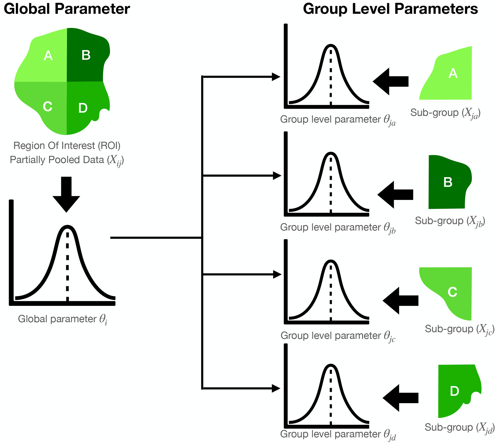
Figure 3An illustration of the parameter structure of the hierarchical Bayesian model based on partially pooled data (Yij). The global parameter (θi) represents the average posterior parameter distribution over an entire region of interest, while the group-level parameters θj(abcd) are the individual posterior parameter distributions inferred from the sub-group data (Yjabc) within the region of interest.
The Bayesian framework used for the parameter inference is based on Bayes' theorem in Eq. (3):
where Xt represents the input data of the ARDL model; P(θ|Xt) represents the probability of our model parameters given our data Xt, also known as the posterior; P(Xt|θ) represents the probability of the data given the parameters, referred to as the likelihood; and P(θ) represents the prior belief about the parameters. P(Xt) is the probability of data or evidence. The evidence is a normalisation term and usually ignored, making the posterior proportional to the likelihood and prior as seen in Eq. (4) (Lambert, 2018; McElreath, 2018).
It is important to note that working with the Bayes' framework allows us to explicitly define our prior beliefs about model parameters. These priors are then updated with the likelihood function to generate the posterior probability distribution when informed by observed data.
The HBM will enable us to fit the ARDL model by simultaneously inferring global parameters (Nodes A and B in Fig. 4) across the partially pooled data as well as their sub-group-level variations (Node G in Fig. 4) (Gelman and Hill, 2006). The sub-group levels, in this case, refer to the different LULCs or AEZs within our data. The varying effect of the sub-groups was incorporated into our HBM as categorical variables (Node K in Fig. 4).
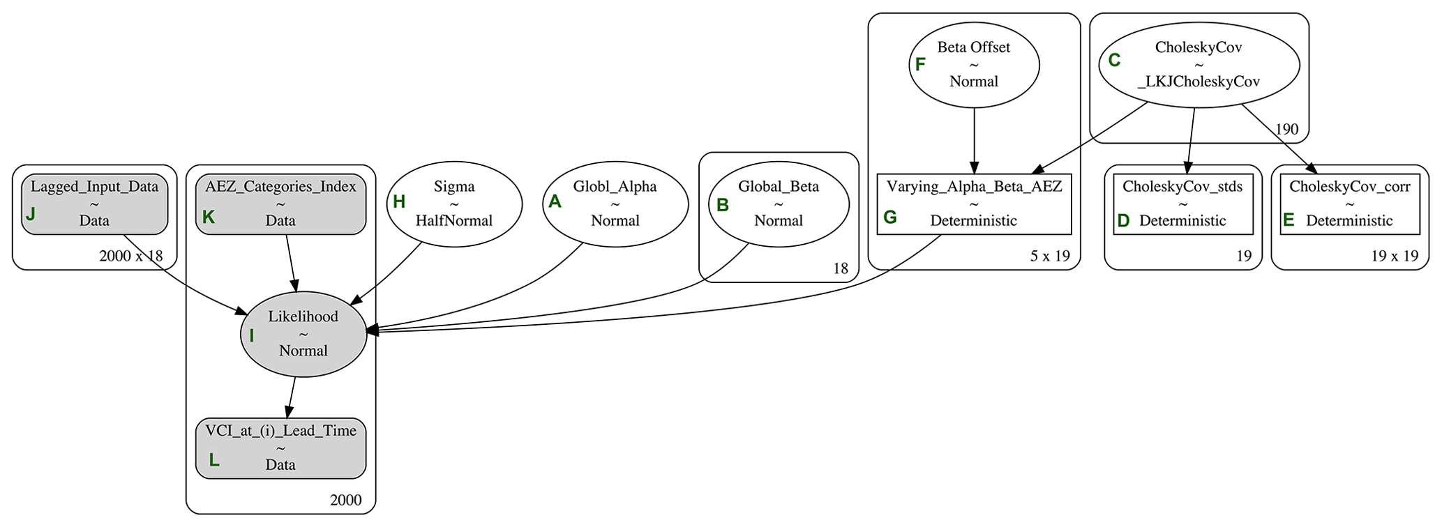
Figure 4A directed acyclic graph (DAG) schema representing the hierarchical model based on varying agro-ecological zones. The figure depicts how the hierarchical model parameters and input data are defined and structured.
The HBM was based on an ARDL (p=6, q=6), where the lagged values of P3M, SM3M, and VCI3M were all set to lags of 6 weeks. The nature of the input variables suggests a high likelihood for our model parameters to have a strong correlation. We addressed this by modelling our group-level parameters as a multivariate normal distribution using a Cholesky matrix decomposition as hyper-priors (prior of a prior distribution) (Nodes C–E in Fig. 4) (McElreath, 2018). The Cholesky factorisation was used to transform the multivariate distribution to increase the efficiency of parameter sampling (Stan Development Team, 2018). The group-level parameters of the HBM are modelled as conditional probabilities of the global parameters; however, these group-level parameters tend to not separate well from the global parameters. When this happens, the model does not converge, resulting in less precise forecasts. We handled this by introducing an offset factor (Node F in Fig. 4) to make the model non-centred (Betancourt and Girolami, 2013). The global parameters were set to follow a normal distribution to enable parameter values to take on positive and negative values. Due to the hierarchical structure of the model parameters, global prior distribution usually serves as hyper-priors for the group-level parameters.
Parameter approximation for the HBM was sampled with the Hamiltonian Monte Carlo (HMC) algorithm (Hoffman and Gelman, 2014), an improved version of the classic Markov Chain Monte Carlo (MCMC) based on the notion of Hamiltonian dynamics. For this research, however, the No-U-Turn Sampler (NUTS) (Hoffman and Gelman, 2014) version of HMC was used.
The hierarchical BARDL model in this study was defined as
where Dt+n is the VCI3M at n weeks ahead, and Dt−q represents the data for lags 0 to q of VCI3M (dependent variable). Pt−p and St−p are the lags 0 to p, P3M, and SM3M, respectively. αj[i] is the global (i) and group-level (j) regression intercept, and βj[d], θj[p], and δj[s] are the regression coefficients for the lagged P3M and SM3M input variables at the global (i) and group level (j). ϵt−p is the regression error term. Equation (5) can be simplified as Eq. (6) and re-written as a Bayesian likelihood function P(Xt|θ) in Eq. (7):
where n is the lead time, βj[i] is the global and group-level model parameters, and Xt−i represents the lagged input variables in Eq. (5).
where , , , and (half-normal distribution).
Below (Fig. 4) is a directed acyclic graph (DAG) schematic representation of an example of the HBM used for this study.
The nodes seen in the HBM DAG in Fig. 4 are defined as follows:
-
Node A is the global (mean) regression intercept or (αi) parameter assumed to be Gaussian.
-
Node B represents global (mean) regression coefficients for each of the lagged input variables (precipitation and soil moisture) or (βi) parameters for the 18 lagged variables (6 lags each for VCI3M, P3M, and SM3M).
-
Node C represents the Cholesky covariance matrix used as hyper-priors for the group-level αj and βj parameters;
-
Nodes D and E are the Cholesky standard deviation and correlation from the matrix decomposition, respectively.
-
Node F represents the offset distribution (Gaussian) hyper-prior to make the model non-centred.
-
Node G is the prior group-level parameters for αj and βj parameters for each vegetation AEZ within our selected counties – i.e. 5 AEZs (βj) within each of the 18 (βi) parameters plus 1 (αi).
-
Node H represents the error term in the HBM regression.
-
Node I is the likelihood function (Eq. 7) of the HBM regression and is based on ARDL (p=6, q=6) shown in Eqs. (5) and (6).
-
Node J is our lagged inputs datasets.
-
Node K is the categorical values that map the input data to their respective AEZs.
-
Node L is the observed VCI3M values at an i lead time.
3.3 Forecasting and model evaluation
The forecast method used in this work was the direct multi-step forecast approach as described by Ben Taieb et al. (2010) and Ben Taieb and Hyndman (2014).
where νi is the model parameters, and Xt−i is the lagged inputs.
With this approach, separate models are fitted for every n lead time forecast. Meaning, for each nth step ahead of a forecast (Dt−n), the observed VCI3M for the training dataset is shifted by n weeks ahead from lag 0 Xt−0 for all input variables.
After the parameter estimation via HMC sampling, the held-out dataset is passed to the fitted model (without the target variable) to produce forecast values for n weeks ahead. The held-out observed values and mean values of our forecast distributions were used to compute the coefficient of determination (R2) (Eq. 10) and root mean square error (RMSE) (Eq. 9) metrics for forecast evaluation. The R2 score quantifies the variation in the observed data that the model could explain, while the RMSE measures the average difference between the observed and forecast values.
where the yi is the observed data, fi is the forecasts, and n is the total number of data points.
where yi is the observed data, and fi is the forecasts.
The forecast uncertainties were analysed with the mean prediction interval width (MPIW) and the prediction interval coverage probability (PICP) (Pang et al., 2018). The PICP computes the percentage of time the observed variable falls within a chosen prediction interval. The MPIW measures the mean distance between the upper (u) and lower (l) bound for a chosen prediction interval.
The MPIW was derived as follows:
where u(Di) and l(Di) are the absolute upper- and lower-bound values of the forecast distribution.
The PICP was derived as follows:
where N is the number of forecast samples, ci is either 0 if the observed drought indicator value at Dt+n falls outside the prediction interval or 1 if the observed value is within the upper and lower bound of the forecast distribution.
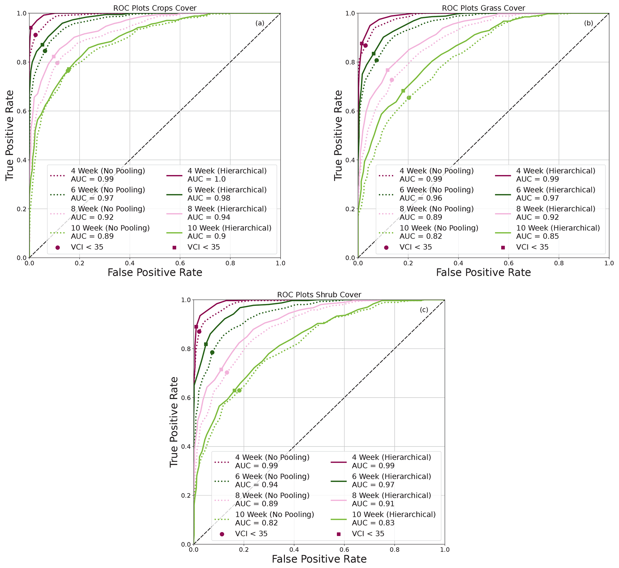
Other forecast verification metrics used in this paper are the receiver operating characteristic (ROC) curve (Wilks, 2006) and forecast probability reliability diagrams and sharpness plots (Wilks, 2006; Jolliffe and Stephenson, 2012).
The ROC curve tells us the likelihood of a forecast being true (true positive rate – TPR) for the given drought threshold and the probability of the forecast event being false (false alarm rate – FAR). In addition, the area under the curve (AUC) was also computed to determine the propensity of our model to separate drought events for the set threshold (Bradley, 1997).
The reliability diagram allows us to assess the accuracy of the forecast probability predicted by our model. The probability of a drought event is computed using the full posterior distribution of our forecasts at a given drought threshold. The same threshold is used to convert observed data into binary events, where 0 indicates a “no drought”, and 1 indicates a “drought” event. The forecast probabilities and observed binaries are binned into probability intervals and used to plot the forecast reliability diagrams. The reliability of the forecast is assessed by the number of times an observed event agrees with a given forecast probability (Wilks, 2006). The sharpness plots, on the other hand, tell the frequency with which a drought event is predicted within a probability bin (WWRP, 2009).
Our dynamic HBM for forecasting VCI3M was tested on datasets based on their AEZs and vegetation land covers. Two models were developed, a BARDL model based on a no-pooling approach as a base model and an HBM based on the partial-pooling approach. The BARDL model was used to forecast VCI3M for the different AEZs, referred to as “BARDL-AEZ”, and different land covers, referred to as “BARDL-LC”. The HBM, which was modelled with partially pooled AEZ data, is referred to as “HBM-AEZ”, and the model-based partially pooled land cover data are referred to as “HBM-LC”. The results shown in this section are a comparison of BARDL-AEZ to HBM-AEZ and BARDL-LC to HBM-LC.
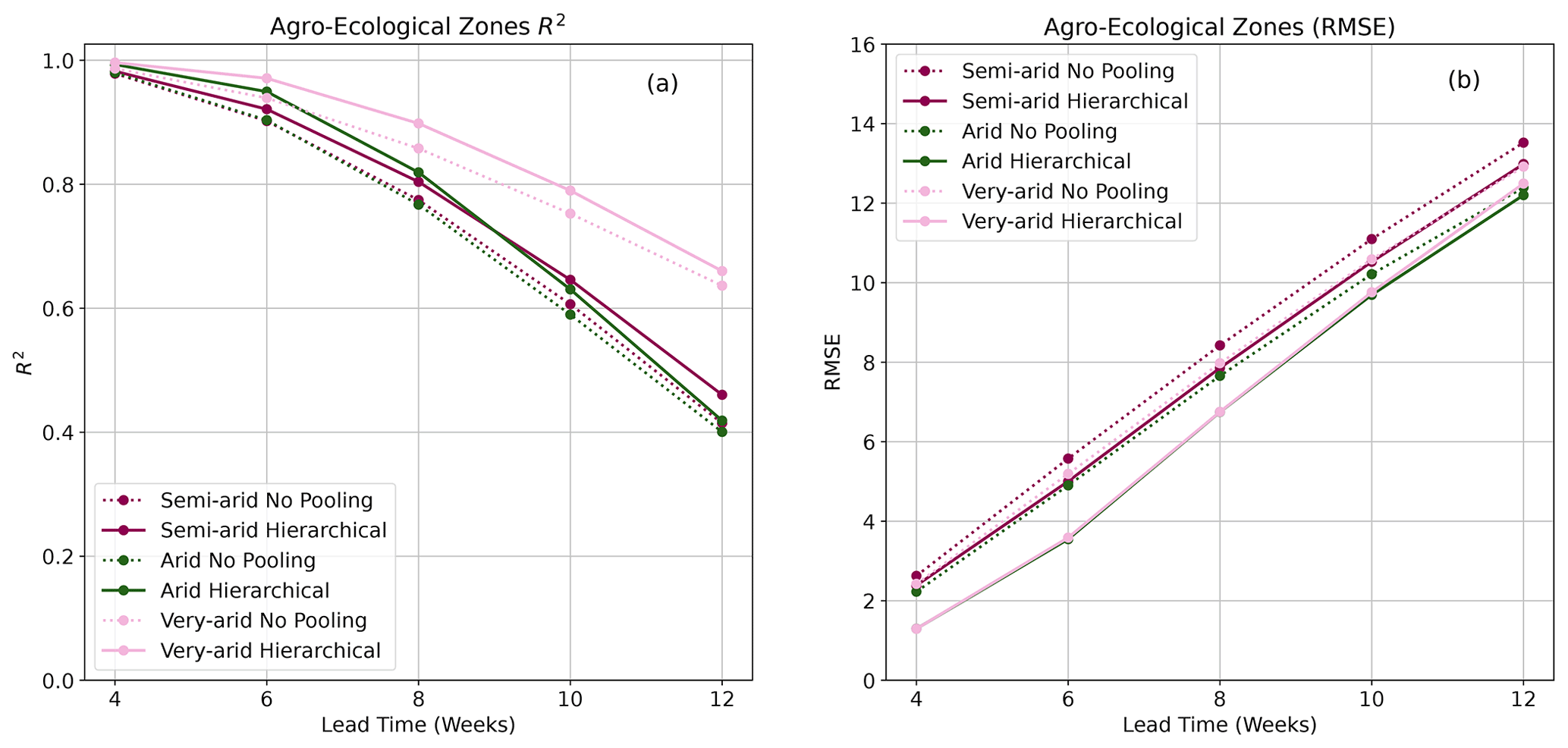
Figure 5Plots showing R2 score (a) and RMSE (b) for BARDL-AEZ (dotted) and HBM-AEZ (solid) and for the VCI3M forecast over the different agro-ecological zones.
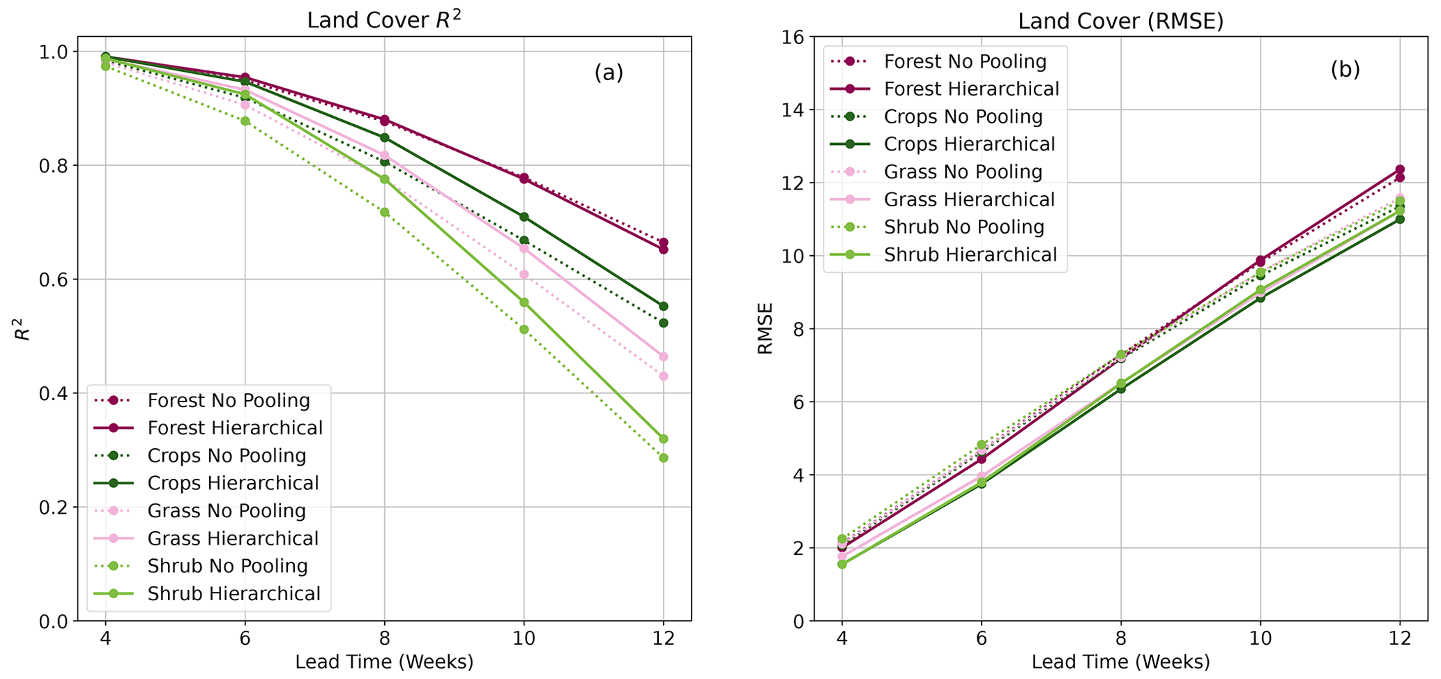
Figure 6Plots showing R2 (a) score and RMSE (b) for BARDL-LC (dotted) and HBM-LC (solid) and for the VCI3M forecast over the different vegetation land cover types.
4.1 Model performance for AEZ-based models
The AEZ-based models were used to forecast VCI3M for the humid, semi-humid, semi-arid, arid, and very arid zones. The R2 scores and RMSE showed in Fig. 5 are for the semi-arid, arid, and very arid zones since they were of most interest. The results for humid zones can be seen in Fig. A1. Both R2 scores and RMSE in Fig. 5a and b showed that the HBM-AEZ model performed better than the BARDL-AEZ model at all the lead times across all the AEZs. The R2 scores were very high for forecasts in the very arid zones, with HBM-AEZ having 0.97, 0.90, and 0.79 compared to 0.93, 0.86, and 0.75 for the BARDL-AEZ at 6-, 8-, and 10-week lead time, respectively. These scores indicate that the HBM was better at capturing the variability within the observed data than the BARDL model. In terms of the forecast errors (RMSE), the HBM-AEZ also performed better than the BARDL-AEZ model, with lower RMSE scores across the lead times.

Figure 7Plots showing R2 (a, c) score and RMSE (b, d) for BARDL-AEZ (dotted) and HBM-AEZ (solid) for the MAM and OND seasons. Panels (a) and (b) are for the MAM season, and panels (c) and (d) are for the OND season.
4.2 Model performance for land-cover-based models
Figure 6 shows the performance metrics for the VCI3M forecast for the vegetation land covers. Overall, the HBM-LC performed better than the BARDL-LC except for the forest covers (where both models had almost identical R2 scores across all lead times). The HBM-LC also performed well up to 10 weeks ahead for cropland, with R2 scores of 0.70 compared to 0.66 for the BARDL model. The R2 score for forecasts over shrublands and grasslands remained between 0.90 and 0.70 up to 8 weeks ahead for the HBM-LC. The forecast errors from the RMSE plot (Fig. 6b) showed a slightly different pattern. The forecast errors for all the land covers except for forest covers were lower for the HBM-LC. There was, however, no difference in R2 and RMSE over forest cover, probably because the group-level effects did not differ significantly from the global effects.
4.3 Model performance during long and short rain seasons
Forecasts by both the HBM-AEZ and the HBM-LC were also evaluated for long rain (March, April, May – MAM) and short rain (October, November, December – OND) seasons. In both seasons, the HBM-AEZ model gave higher forecast accuracies across all lead times as seen in Fig. 7. During the OND season, where drought events mostly occur, forecasts in the arid and very arid zones showed high R2 scores till a lead time of 10 weeks (Fig. 7c), and RMSE stayed below 10 until 12 weeks (see Fig. 7d). The HBM-LC on the other hand only shows significant improvements for the forest and cropland covers in the MAM season. During the OND season, only forecasts over the croplands showed very significant differences (see Fig. B1).
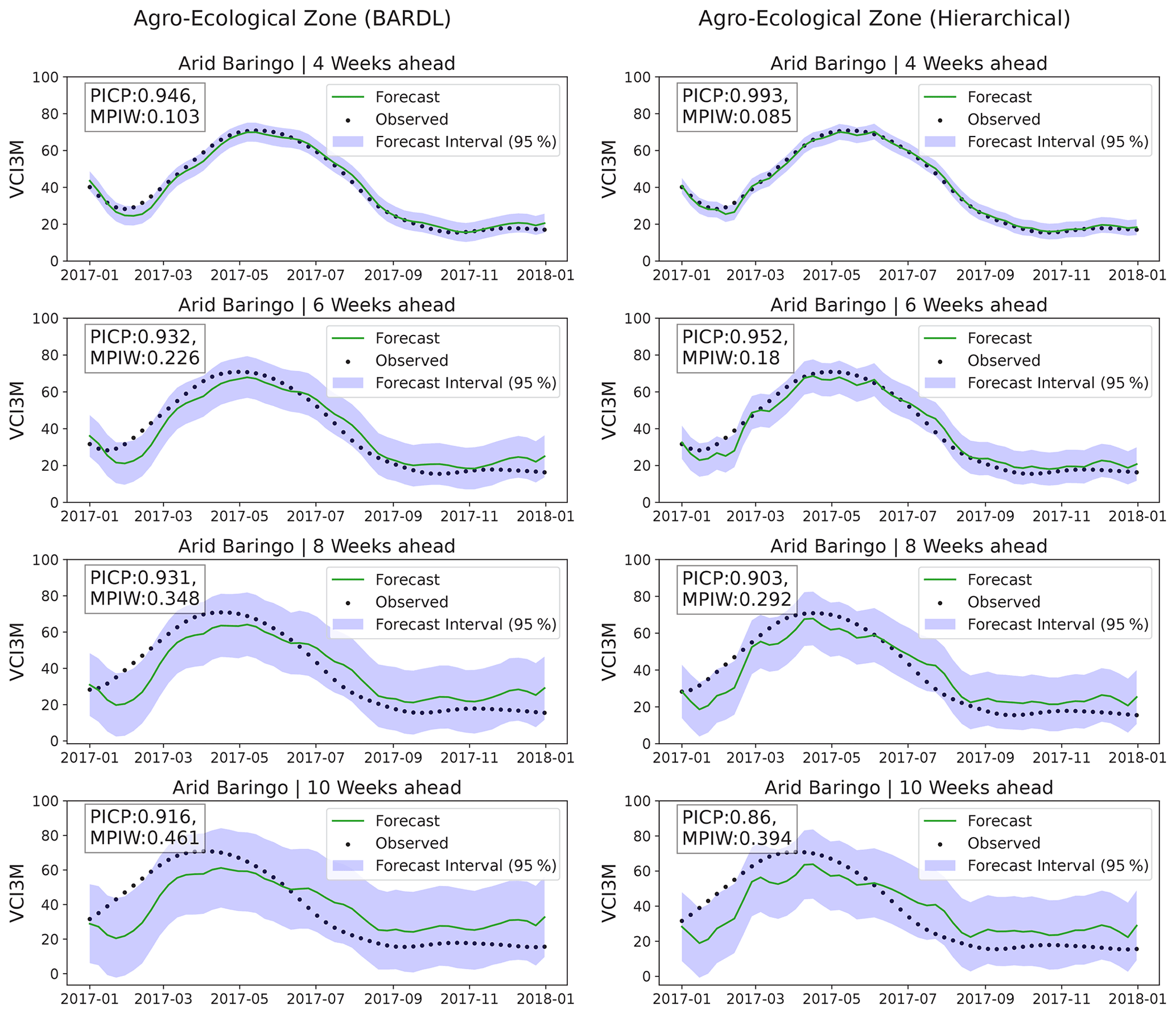
Figure 8Plots showing forecast for arid zones for 4- and 10-week lead times and their uncertainties (PICP and MPIW).
4.4 Uncertainty analysis
The forecast uncertainty in both forecast models was analysed using the PICP and MPIW. The desired PICP value usually ranges between 0.90 and 0.99 (Pang et al., 2018). The PICP indicates the number of times observed values fall within our forecast interval. On the other hand, the MPIW values show forecast precision and are expected to remain very low. Figure 8 shows the time series plots of forecast and observed VCI3M for the arid zone in Baringo County. Each plot shows the 95 % prediction interval along with the PICP and MPIW for 4- to 10-week lead time. The PICP values for both models indicate that observed values for all the lead times fall within a 95 % credible interval of our forecast distributions over 90 % of the time. The high PICP seen for the BARDL model from 8 weeks was due to the wider forecast interval (error bars). A closer look at the MPIW values indicates that the HBM-AEZ forecasts are more precise than BARDL-AEZ, indicating that forecasts from HBM-AEZ have reduced uncertainties. A similar trend was seen for forecasts across all land covers. Overall, the MPIW metrics reiterate that forecasts by the HBM have lower errors than the BARDL. In addition, the partially pooled parameters also indicate errors from the HBM are a better representation of the actual forecast error. Thus, even though PICP from 10 weeks ahead seems high for the BARDL model, it does not reflect the truth.
The mean PICP and MPIW for both AEZs and land covers over the selected counties are in Tables C1 and C2.
4.5 Predicting drought event (ROC curves)
Although our models produce accurate VCI3M values at the various lead times, our target users are also interested in whether or not a drought event alarm will be triggered at a defined threshold. Therefore, the skill of the forecast models at predicting drought events was assessed with the ROC curve with a threshold of VCI3M < 35 %. VCI3M values below this threshold depict moderate to severe drought conditions (Klisch and Atzberger, 2016).
The ROC plots in Fig. 9 show the TPR (hit rate) and FAR (false alarm) for the three arid zones. The dot on the curves indicates the VCI3M < 35 threshold. Apart from the very arid zones (Fig. 9c), significant differences were seen between TPR and FAR for drought events predicted by the HBM-AEZ compared to the BARDL-AEZ (Fig. 9a and b) at all lead times. The hit rates for the HBM-AEZ were higher than the BARDL-AEZ and were mostly above 80 % for drought events from 4 to 10 weeks ahead in the arid areas (Fig. 9b) with false alarm rates between 1 % and 18 %. Drought events in semi-arid zones also had hit rates above 80 % up until 8 weeks (Fig. 9b). Both models performed very well at detecting moderate to severe drought events in the very arid zones, as seen in Fig. 9c, which was mostly because of the frequent occurrence of drought events in the very arid zones.
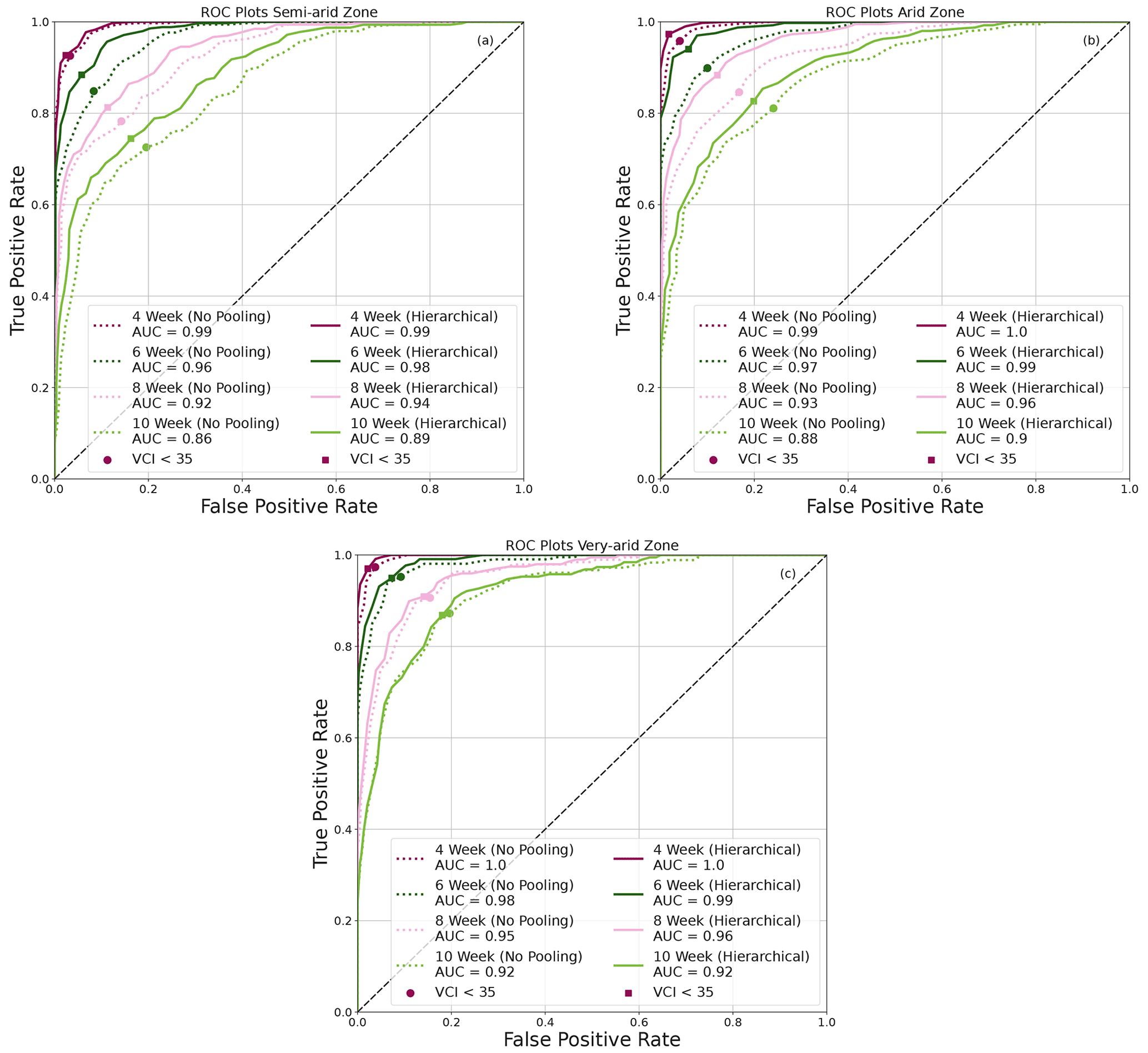
Figure 9ROC plots generally showing higher hit rates for HBM in semi-arid, arid, and very arid zones.
Figure 10 shows the ROC plots for the croplands, grasslands, and shrubs for the BARDL-LC compared to HBM-LC. Overall, drought events predicted by the HBM-LC also had higher hit rates with lower false alarm rates than the BARDL-LC model. The hit rates for drought events over croplands remained above 80 % up to 10 weeks ahead, with false alarm rates ranging between 1 % and 16 %. The TPR for grasslands and shrubs dropped quickly after 6 weeks. The TPRs were generally above 60 % for all land covers at all lead times.
4.6 Forecast reliability
The reliability plots in Fig. 11 are a joint distribution of the binned forecast probabilities and relative frequency of the actual observed drought event (observed binaries = 1) for their respective probability bins. In a perfect system, the joint plots should lie on the diagonal line. The plots also show a histogram that depicts the model's sharpness. A perfect sharpness plot should have peaks at the extreme ends of the histogram. A peak close to the 0 % probability bin indicates the frequency at which the model predicted a “no drought” event, whereas a peak close to the 100 % probability bin means otherwise. It is essential to state that a forecast system is said to exhibit little or no sharpness when a sharpness peak is close to the long-term mean or climatology (Jolliffe and Stephenson, 2012).

Figure 11Reliability and sharpness plots showing a joint distribution of forecast probabilities and observed frequencies for various arid and very arid agro-ecological zones for the different lead times.
The reliability diagrams for both BARDL-AEZ and HBM-AEZ (Fig. 11) showed some differences but were not very significant. The proximity of the reliability curves to the diagonal line, especially for the arid zones (Fig. 11a and c), indicates that the forecast probabilities from both models can be trusted for early warning and early action. From Fig. 11a, we see that when the BARDL-AEZ model predicts a drought event with a probability ranging between 80 % and 100 % 4 to 6 weeks ahead, the forecast probability agrees with the observed frequency 90% to 99% of the time, which can also be seen in Fig. 11c for the HBM-AEZ model. For the very arid zones, forecast probabilities between 60 % and about 80 % (Fig. 11b and d) corresponded to very high observed relative frequencies above 80 %, a situation referred to as “under-forecasting”. Under-forecasting describes the situation where forecast probabilities do not adequately reflect observed events (Wilks, 2006). However, a closer look shows some subtle improvements with the HBM-AEZ, with a slight difference in the under-forecasting effect from 4- to 6-week lead times. Regarding the sharpness of the models, a higher frequency of drought events was seen in the higher forecast probability bin for the HBM-AEZ (Fig. 11c and d) compared to the BARDL-AEZ (Fig. 11a and b), especially from 6 to 12 weeks in the arid zone. The reliability diagrams for croplands and grasslands for both BARDL-LC and HBM-LC models also showed similar patterns. Please see Fig. D1 in Appendix C.
The skill of the models at predicting the onset and end of a drought period can be seen in Fig. 12. The figure shows a time series plot of observed and forecasted VCI3M at a 4-week lead time in a very arid zone within Turkana County of Kenya for 2017. The plot also shows the forecast probability as a dot on vertical lines depicting the onset and end of a drought period. We can see from Fig. 12a that at the start of a drought period where the observed VCI3M dropped below the threshold (VCI3M < 35) line, the forecasted probability for the drought event predicted by the BARDL-AEZ was 9.4 %. The low probability was because the forecasted VCI3M model value was higher than the observed value and threshold. However, the likelihood of a drought onset predicted by the HBM-AEZ in Fig. 12b was 73 %, prompting a trigger for early action. Towards the end of the drought period, the BARDL-AEZ model gave a high drought probability even though the drought duration had ended. Although these differences are not seen in all cases at the onset and end of a drought period, the few occurrences in some regions of interest emphasise that HBMs provide a better approach to forecasting VCI3M over a diverse region.
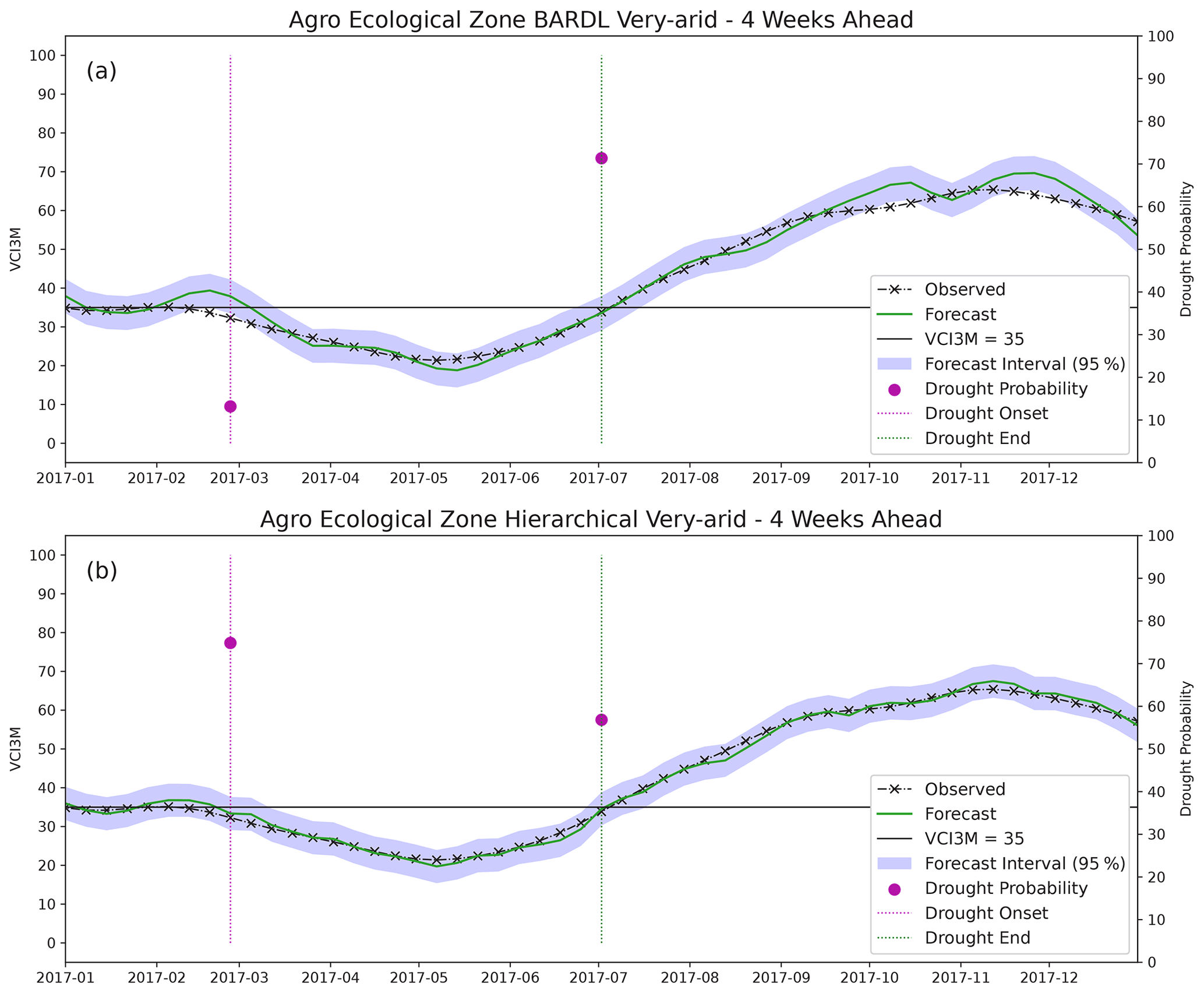
Figure 12A time series plot showing the observed and forecasted VCI3M for the period of 2017. Forecast probabilities are indicated as points on the horizontal lines marking the onset and end of a drought period.
4.7 Test transfer learning
Although the data used for training and developing forecast models are usually sampled to represent a given area of interest, the goal in most cases is to have models that can scale up to produce forecasts over more expansive areas. The second objective of this study was to test the transfer learning capability of HBMs over other regions. The partially pooled data used for hierarchical parameter approximations were sampled from six counties. The trained models for the different lead times were then used to forecast VCI3M for the AEZs and land covers over 10 additional counties (shown with black boundaries in Fig. 2), which were not part of the training sets. The comparison of their R2 and RMSE metrics in Fig. 13 proved that both HBMs were able to forecast VCI3M over the non-trained counties accurately. For the AEZs, some significant differences were seen between the trained and non-trained counties in the semi-arid zones in terms of explained variances (R2 score) (Fig. 13a). The case was different for forecast error in the same zone as seen in Fig. 13b. A significant gap was also seen for the forecast error over the very arid area but not for the explained variances. Performance over the different land covers, however, remained very close, especially for the RMSE (Fig. 13d) despite the gap seen for grassland in the R2 score plots (Fig. 13c). These differences can be linked to the fact that although some non-trained counties may have similar AEZs or land covers, their climatic and vegetation phonology cycles are not similar. Aside from these observed differences, the HBMs could generalise and accurately forecast when given new unseen data.
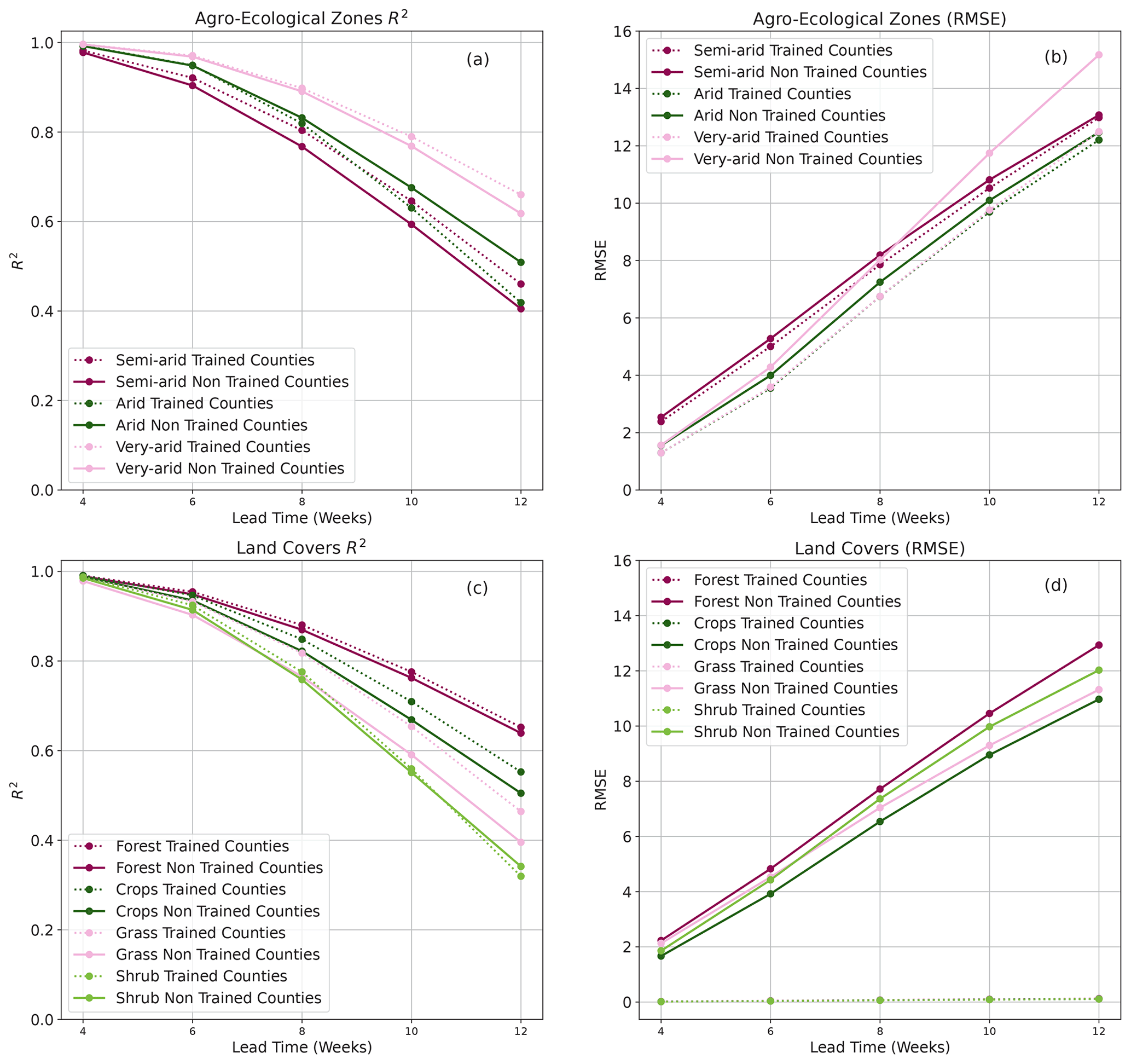
Figure 13Plot showing R2 score and RMSE for forecasts over counties not included in the training data (solid lines) used for the HBM versus the counties included in the training data (dotted lines).
In this paper, we seek to improve the forecast accuracy of VCI3M over vast areas with varying AEZs and land covers using an HBM. Compared to the non-hierarchical BARDL model, the HBM presented a more realistic approach for forecasting VCI3M in regions with different AEZs or land covers. The evaluation of the HBM based on R2 metrics indicated that forecasts over the very arid zones and forest cover areas showed higher accuracies at longer lead times. The high accuracy observed for the very arid zones could be a consequence of the significant contribution from the lagged soil moisture to future VCI3M in addition to precipitation as seen in Figs. E1 and F1. For the forest areas, the observation could be because some dense forests show slight variation during drought periods.
The strong relationship between lagged soil moisture VCI3M over forest areas could be due to the frequent precipitation and high soil moisture retention in areas as seen in Fig. F1. On the other hand, the low contribution of soil moisture to forecasts in croplands, grasslands, and shrubs could be attributed to the low soil moisture levels over grass and shrub areas (James et al., 2003; Tyagi et al., 2013). For croplands, the low contribution of soil moisture could be due to several factors, including high temperature and soil type. However, in the very arid areas, the high relative importance of soil moisture could be due to the rapid response of vegetation to sudden increases in soil moisture, especially after long periods of dryness (see Fig. E1).
Overall, results from the various skill assessments showed that forecasts with HBM were more precise, with a lower false alarm rate for drought events than the BARDL model. The HBM was also able to effectively identify drought events in counties with diverse AEZs and some land covers. The HBM also performed well in both the long and short rain seasons for the arid and very arid AEZs, which are more prone to drought occurrences.
Relating the overall forecast skill assessments from this work to previous works, the HBM showed an approximately 1-week increase in the forecast range compared to the results from the BARDL method used in Salakpi et al. (2022). On average, the HBM also exhibited an approximately 2-week increase in forecast range, compared to the auto-regression method used in Salakpi et al. (2022) and Barrett et al. (2020). Furthermore, using the HBM also enabled the simultaneous forecast of VCI3M for different AEZs and land covers, which we could not do with the methods used in Salakpi et al. (2022) and Barrett et al. (2020). Finally, despite the improvement seen with the HBM, the BARDL models also proved to be useful at predicting drought events at the set threshold as demonstrated by Salakpi et al. (2022).
Aside from the improvement in the forecast range, the HBM also had some added strengths. First of all, the hierarchical nature of the model parameters (see Fig. 3) enabled the incorporation of the varying (AEZ or land cover) effects of climate and other biophysical factors on vegetation conditions. Thus, modelling within the HBM framework made it possible to learn the within-sample parameters in addition to the global parameters and accurately forecast VCI3M values specific to the AEZs and land covers. Secondly, modelling within a Bayesian context means the model outputs probability distributions instead of point values. These distributions present a direct approach to quantifying forecast uncertainties. The probability distribution of forecasts also made it possible to derive forecast probabilities, which allowed us to quantify the likelihood of drought events in different locations. Finally, the HBM also makes it possible to transfer trained models to similar datasets that were not part of the initial training data. Transferring the model also means that, even though the HBM model was calibrated on the data from Kenya, it can be scaled up to generate forecasts for wider regions without the need to re-calibrate.
The threat of agricultural drought to food security and global economies has pushed agencies like the USAID and FAO to develop early warning systems that continually monitor drought events. However, agricultural drought over vast and diverse arid and semi-arid lands (ASAL) regions poses a challenge to effective monitoring (Boken et al., 2005; Vicente-Serrano, 2006). Policy- and decision-makers at these agencies, including Kenya's National Drought Management Authority (NDMA), our primary stakeholder, can incorporate the HBM demonstrated in this paper into their existing early warning systems to enhance their efforts. Aside from accounting for the different AEZs or land covers, the forecasted drought probabilities from the HBM will also enable intelligent decision-making for drought relief agencies that practise forecast-based financing (FbF) (Coughlan de Perez et al., 2015) for drought early action.
The methods used in this paper also had a few limitations. A fundamental limitation was the timely availability of the ESA CCI soil moisture data, a setback that can affect the prospects of producing real-time forecasts. Parameter inference via the HMC sampler also takes a long time to complete partly due to the complex nature of the HBM and the number of data points involved. However, this was not considered to be a significant limitation as it only occurs during the model training phase. Once the model converges, and sampling completes, the posterior predictive sampling or forecasting of VCI3M takes seconds.
In this paper, we present a proof of concept that HBM can factor spatial differences into drought forecasting. Using this approach also allowed us to understand the vegetation dynamics in agro-climatic areas and regions with diverse vegetation covers. For instance, we saw an approximately 1-week gain in forecast range for vegetation conditions in very arid areas as well as forests (tree cover) and cropping areas. Furthermore, we show that soil moisture contributes more when forecasting VCI3M over very arid areas and forest covers. However, future work on drought forecasting should explore other indicators like the vegetation health indicator (VHI) or VCI based on the soil adjusted vegetation index (SAVI) instead of NDVI as demonstrated by Bowell et al. (2021). Other factors that may directly affect agriculture drought like atmospheric evaporative demand (Vicente-Serrano et al., 2020) should also be considered.
We also show that HBM trained with data in one area could be transferred to other similar datasets in other regions. Future research work should consider more complex HBMs that take into account variations for different land cover types within the various agro-ecological zones and the seasonal differences.

Figure A1Plots showing R2 score and RMSE for BARDL-AEZ (dotted) and HBM-AEZ (solid) and for the VCI3M forecast over the different humid zones.
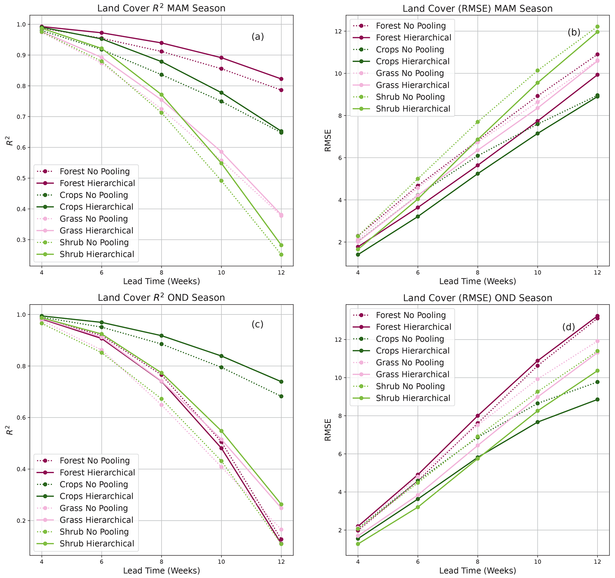
Figure B1Plots showing R2 ((a, c) score and RMSE (b, d) for BARDL-LC (dotted) and HBM-LC (solid) for the MAM and OND seasons. Panels (a) and (b) are for the MAM season, and panels(c) and (d) are for the OND season.
Table C1Table showing a PICP and MPIW (in parentheses) for the various agro-ecological zones.

Table C2Table showing a PICP and MPIW (in parentheses) for the various vegetation land covers.
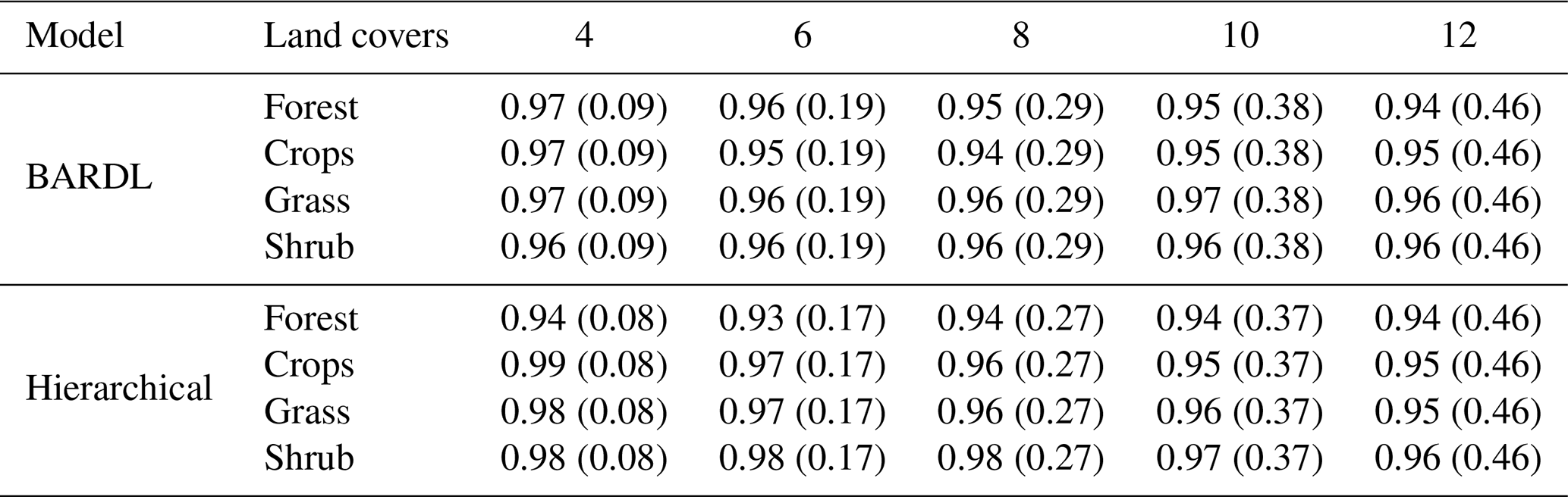
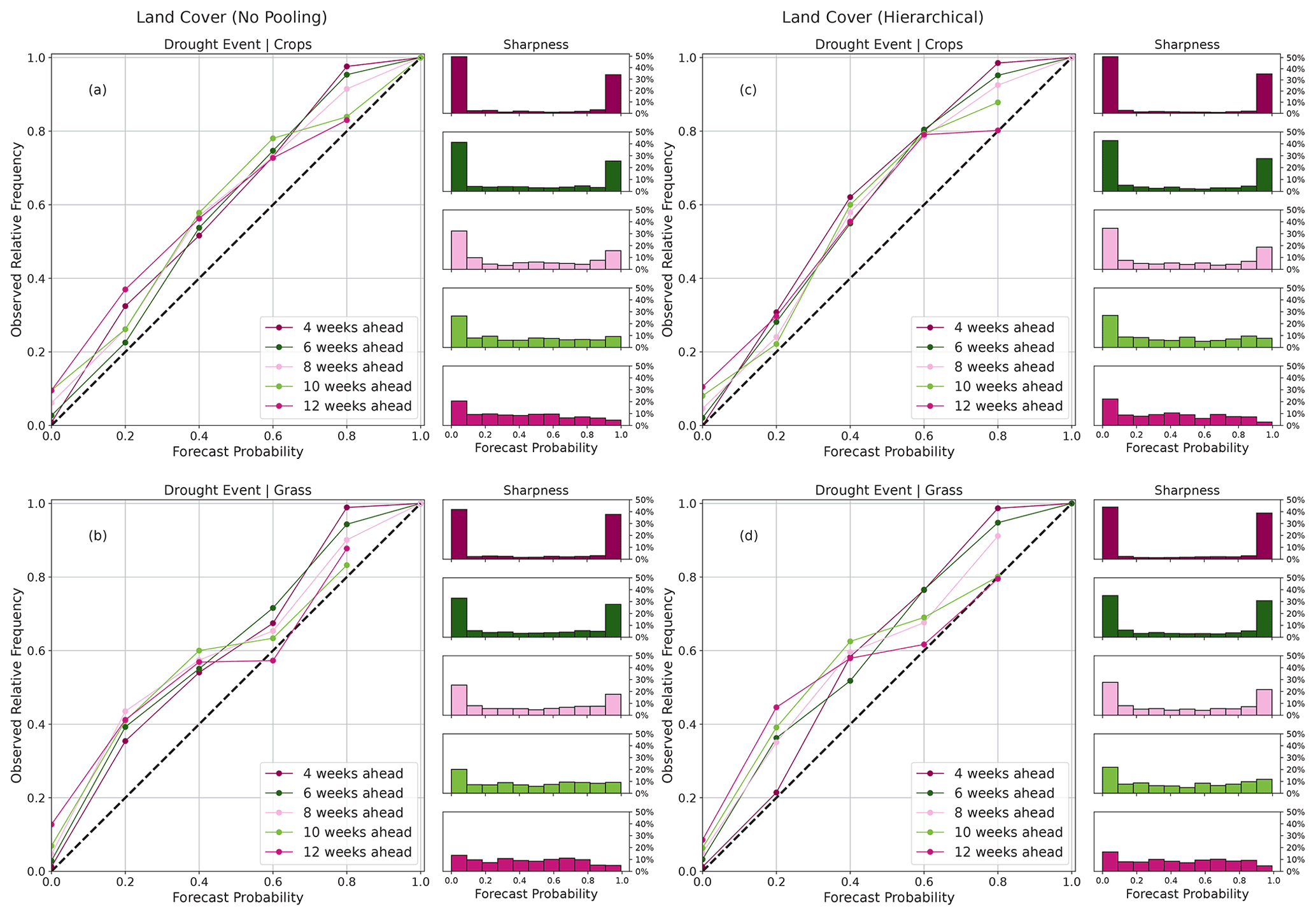
Figure D1Reliability and sharpness plots showing a joint distribution of forecast probabilities and observed frequencies for various agro-ecological zones and land cover for different lead times.
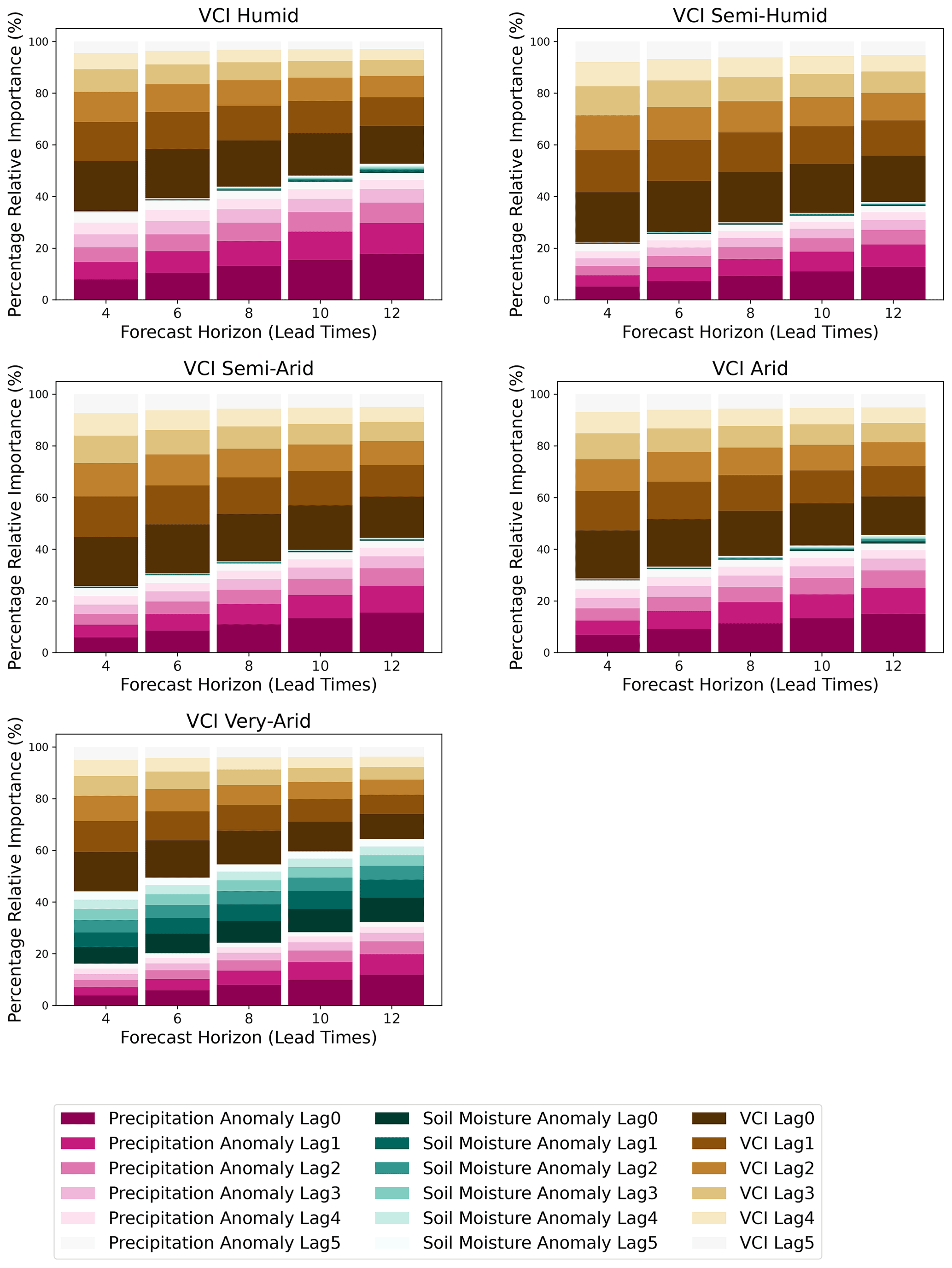
Figure E1Plots showing the relative importance of the lagged input variables (VCI3M, P3M, SM3M) and VCI3M at 4- to 12-week lead times for the different agro-ecological zones.
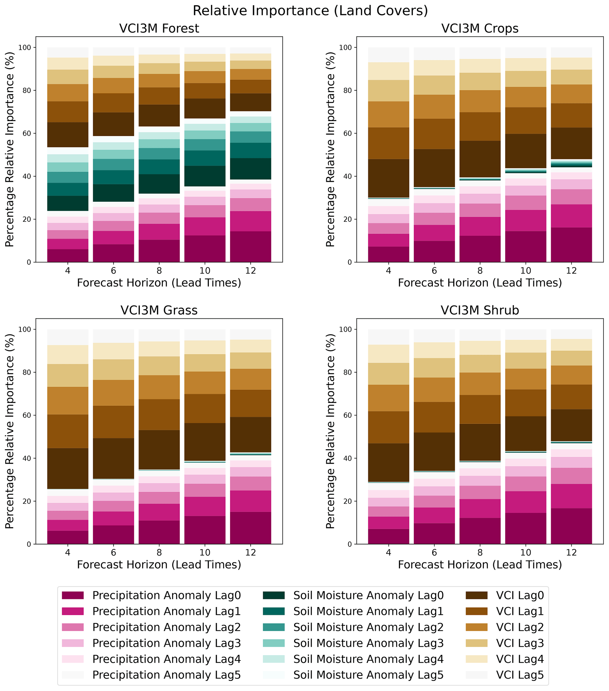
Figure F1Plots showing the relative importance of the lagged input variables (VCI3M, P3M, SM3M) and VCI3M at 4- to 12-week lead times for the different vegetation land covers.
The data and code repository can be found here: https://doi.org/10.5281/zenodo.7005178 (Salakpi and Bowel, 2022).
EES is the lead author and was responsible data pre-processing, modelling (coding), and running BARDL and HBM. JMM assisted with data acquisition, pre-processing, cartography, and feedback. AB developed the code for the smoothing algorithm used for the time series data. SO, PR, and PH conceptualised the initial idea and provided supervision and feedback. The final manuscript was edited and reviewed by all authors.
The contact author has declared that none of the authors has any competing interests.
Publisher's note: Copernicus Publications remains neutral with regard to jurisdictional claims in published maps and institutional affiliations.
The work was funded by the UK Newton Fund's Development in Africa with Radio Astronomy (DARA) Big Data project delivered via STFC with grant number ST/R001898/1 and by the Science for Humanitarian Emergencies and Resilience (SHEAR) consortium project “Towards Forecast-based Preparedness Action” (ForPAc; https://sites.google.com/view/forpac-shear/home, last access: 3 October 2021), grant number NE/P000673/1, funded by the UK Natural Environment Research Council (NERC), the Economic and Social Research Council (ESRC), and the UK Department for International Development (DfID).
This research has been supported by the Newton Fund (grant no. ST/R001898/1) and the Natural Environment Research Council (grant no. NE/P000673/1).
This paper was edited by Maria-Carmen Llasat and reviewed by three anonymous referees.
Adede, C., Oboko, R., Wagacha, P. W., and Atzberger, C.: A Mixed Model Approach to Vegetation Condition Prediction Using Artificial Neural Networks (ANN): Case of Kenya's Operational Drought Monitoring, Remote Sens., 11, 1099, https://doi.org/10.3390/rs11091099, 2019. a
Asaad, A.-A. B. and Magadia, J. C.: Stochastic Gradient Hamiltonian Monte Carlo on Bayesian Time Series Modeling, in: 14th National Convention on Statistics Crowne Plaza Manila Galleria, 1–3 October 2019, Ortigas Center, Quezon City, 2019. a
Ayugi, B. O., Wen, W., and Chepkemoi, D.: Analysis of Spatial and Temporal Patterns of Rainfall Variations over Kenya, 6, https://www.iiste.org/ (last access: 3 October 2021), 2016. a
Barrett, A. B., Duivenvoorden, S., Salakpi, E. E., Muthoka, J. M., Mwangi, J., Oliver, S., and Rowhani, P.: Forecasting vegetation condition for drought early warning systems in pastoral communities in Kenya, Remote Sens. Environ., 248, 111886, https://doi.org/10.1016/j.rse.2020.111886, 2020. a, b, c
Ben Taieb, S. and Hyndman, R. J.: Recursive and direct multi-step forecasting: the best of both worlds, https://citeseerx.ist.psu.edu/viewdoc/download?doi=10.1.1.375.7885&rep=rep1&type=pdf (last access: 14 August 2022), 2014. a
Ben Taieb, S., Sorjamaa, A., and Bontempi, G.: Multiple-output modeling for multi-step-ahead time series forecasting, Neurocomputing, 73, 1950–1957, https://doi.org/10.1016/j.neucom.2009.11.030, 2010. a
Betancourt, M. J. and Girolami, M.: Hamiltonian Monte Carlo for Hierarchical Models, Current Trends in Bayesian Methodology with Applications, arxiv: preprint, 79–101, http://arxiv.org/abs/1312.0906, 2013. a
Bishop, C. M. and Nasrabadi, N. M.: Pattern recognition and machine learning, in: Vol. 4, Springer, New York, p. 738, ISBN 978-1-4939-3843-8, 2006. a, b
Boken, V. K., Cracknell, A. P., and Heathcote, R. L.: Monitoring and Predicting Agricultural Drought, Oxford University Press, https://doi.org/10.1093/oso/9780195162349.001.0001, 2005. a, b, c, d, e
Bowell, A., Salakpi, E. E., Guigma, K., Muthoka, J. M., Mwangi, J., and Rowhani, P.: Validating commonly used drought indicators in Kenya, Environ. Res. Lett., 16, 084066, https://doi.org/10.1088/1748-9326/ac16a2, 2021. a
Bradley, A. P.: The use of the area under the ROC curve in the evaluation of machine learning algorithms, Pattern Recognit., 30, 1145–1159, https://doi.org/10.1016/S0031-3203(96)00142-2, 1997. a
Coughlan de Perez, E., van den Hurk, B., van Aalst, M. K., Jongman, B., Klose, T., and Suarez, P.: Forecast-based financing: an approach for catalyzing humanitarian action based on extreme weather and climate forecasts, Nat. Hazards Earth Syst. Sci., 15, 895–904, https://doi.org/10.5194/nhess-15-895-2015, 2015. a
Da Silva, I. N., Spatti, D. H., Flauzino, R. A., Liboni, L. H. B., and dos Reis Alves, S. F.: Artificial neural network architectures and training processes, in: Artificial neural networks, Springer, Cham, 21–28, ISBN 978-3-319-43162-8, https://doi.org/10.1007/978-3-319-43162-8_2, 2017. a
Deleersnyder, R.: Pastoralism in East Africa: challenges and solutions | Glo.be, https://www.glo-be.be/index.php/en/articles/pastoralism-east-africa-challenges-and-solutions (last access: 3 October 2021), 2018. a
Dorigo, W., Wagner, W., Albergel, C., Albrecht, F., Balsamo, G., Brocca, L., Chung, D., Ertl, M., Forkel, M., Gruber, A., Haas, E., Hamer, P. D., Hirschi, M., Ikonen, J., de Jeu, R., Kidd, R., Lahoz, W., Liu, Y. Y., Miralles, D., Mistelbauer, T., Nicolai-Shaw, N., Parinussa, R., Pratola, C., Reimer, C., van der Schalie, R., Seneviratne, S. I., Smolander, T., and Lecomte, P.: ESA CCI Soil Moisture for improved Earth system understanding: State-of-the art and future directions, Remote Sens. Environ., 203, 185–215, https://doi.org/10.1016/j.rse.2017.07.001, 2017. a
Eilers, P. H. C.: A Perfect Smoother, Anal. Chem., 75, 3631–3636, https://doi.org/10.1021/ac034173t, 2003. a
FEWSNET: About Us | Famine Early Warning Systems Network, https://fews.net/about-us, last access: 3 October 2021. a
Fischer, G., van Velthuizen, H., and Nachtergaele, F.: Global Agro-Ecological Zones Assessment: Methodology and Results, https://pure.iiasa.ac.at/id/eprint/6182/1/IR-00-064.pd (last acess: 18 August 2022), 2000. a
Funk, C., Peterson, P., Landsfeld, M., Pedreros, D., Verdin, J., Shukla, S., Husak, G., Rowland, J., Harrison, L., Hoell, A., and Michaelsen, J.: The climate hazards infrared precipitation with stations – A new environmental record for monitoring extremes, Scient. Data, 2, 1–21, https://doi.org/10.1038/sdata.2015.66, 2015. a
Funk, C., Shukla, S., Thiaw, W. M., Rowland, J., Hoell, A., McNally, A., Husak, G., Novella, N., Budde, M., Peters-Lidard, C., Adoum, A., Galu, G., Korecha, D., Magadzire, T., Rodriguez, M., Robjhon, M., Bekele, E., Arsenault, K., Peterson, P., Harrison, L., Fuhrman, S., Davenport, F., Landsfeld, M., Pedreros, D., Jacob, J. P., Reynolds, C., Becker-Reshef, I., and Verdin, J.: Recognizing the Famine Early Warning Systems Network: Over 30 Years of Drought Early Warning Science Advances and Partnerships Promoting Global Food Security, B. Am. Meteorol. Soc., 100, 1011–1027, https://doi.org/10.1175/BAMS-D-17-0233.1, 2019. a
Gebremeskel, G., Tang, Q., Sun, S., Huang, Z., Zhang, X., and Liu, X.: Droughts in East Africa: Causes, impacts and resilience, Earth-Sci. Rev., 193, 146–161, https://doi.org/10.1016/j.earscirev.2019.04.015, 2019. a
Gelman, A. and Hill, J.: Data analysis using regression and multilevel/hierarchical models, Cambridge University Press, ISBN 9781139460934, 1139460935, 2006. a, b, c, d, e
Gelman, A., Carlin, J. B., Stern, H. S., Dunson, D. B., Vehtari, A., and Rubin, D. B.: Bayesian data analysis, CRC Press, https://doi.org/10.1201/9780429258411, 2013. a, b, c
George, D. and Hawkins, J.: A hierarchical Bayesian model of invariant pattern recognition in the visual cortex, in: vol. 3, , Proceedings 2005 IEEE International Joint Conference on Neural Networks, 1812–1817, https://doi.org/doi:10.1109/IJCNN.2005.1556155, 2005. a
Gruber, A., Scanlon, T., Van Der Schalie, R., Wagner, W., and Dorigo, W.: Evolution of the ESA CCI Soil Moisture climate data records and their underlying merging methodology, Earth Syst. Sci. Data, 11, 717–739, https://doi.org/10.5194/essd-11-717-2019, 2019. a
Gujarati, D.: Basic Econometrics, Economic series, McGraw Hill, https://books.google.co.uk/books?id=byu7AAAAIAAJ (last access: 3 October 2021), 2003. a, b
Heim Jr., R. R.: A Review of Twentieth-Century Drought Indices Used in the United States, B. Am. Meteorol. Soc., 83, 1149–1166, 2002. a
Hoffman, M. D. and Gelman, A.: The No-U-Turn Sampler: Adaptively Setting Path Lengths in Hamiltonian Monte Carlo, J. Mach. Learn. Res., 15, 1593–1623, 2014. a, b
IISD: WMO Checklist Helps Enhance Early Warning Systems | News | SDG Knowledge Hub | IISD, https://sdg.iisd.org/news/wmo-checklist-helps-enhance-early-warning-systems/ (last access: 3 October 2021) 2018. a
James, S. E., Pärtel, M., Wilson, S. D., and Peltzer, D. A.: Temporal heterogeneity of soil moisture in grassland and forest, J. Ecol., 91, 234–239, https://doi.org/10.1046/J.1365-2745.2003.00758.X, 2003. a
Jolliffe, I. T. and Stephenson, D. B.: Forecast verification: a practitioner's guide in atmospheric science, John Wiley & Sons, ISBN 9781119961079, 1119961076, 2012. a, b
Klisch, A. and Atzberger, C.: Operational drought monitoring in Kenya using MODIS NDVI time series, Remote Sens., 8, 267, https://doi.org/10.3390/rs8040267, 2016. a, b
Kogan, F. N.: Application of vegetation index and brightness temperature for drought detection, Adv. Space Res., 15, 91–100, https://doi.org/10.1016/0273-1177(95)00079-T, 1995. a
Lal, R.: Climate Change and Soil Degradation Mitigation by Sustainable Management of Soils and Other Natural Resources, Agricult. Res., 1, 199–212, https://doi.org/10.1007/s40003-012-0031-9, 2012. a
Lambert, B.: A Student's Guide to Bayesian Statistics, SAGE Publications, ISBN 9781526418289, 1526418282, 2018. a
McElreath, R.: Statistical Rethinking: A Bayesian Course with Examples in R and Stan, Chapman & Hall/CRC Texts in Statistical Science, CRC Press, https://doi.org/10.1201/9780429029608, 2018. a, b
Nay, J., Burchfield, E., and Gilligan, J.: A machine-learning approach to forecasting remotely sensed vegetation health, Int. J. Remote Sens., 39, 1800–1816, https://doi.org/10.1080/01431161.2017.1410296, 2018. a
Nicolai-Shaw, N., Zscheischler, J., Hirschi, M., Gudmundsson, L., and Seneviratne, S. I.: A drought event composite analysis using satellite remote-sensing based soil moisture, Remote Sens. Environ., 203, 216–225, https://doi.org/10.1016/j.rse.2017.06.014, 2017. a
Pang, J., Liu, D., Peng, Y., and Peng, X.: Optimize the coverage probability of prediction interval for anomaly detection of sensor-based monitoring series, Sensors (Switzerland), 18, 967, https://doi.org/10.3390/s18040967, 2018. a, b
Ravines, R., Schmidt, A., and Migon, H.: Revisiting distributed lag models through a Bayesian perspective, Appl. Stoch. Model. Business Indust., 22, 193–210, https://doi.org/10.1002/asmb.628, 2006. a
Rippa, S.: An algorithm for selecting a good value for the parameter c in radial basis function interpolation, Adv. Comput. Math., 11, 193–210, https://doi.org/10.1023/A:1018975909870, 1999. a
Rosenstein, M. T., Marx, Z., Kaelbling, L. P., and Dietterich, T. G.: To transfer or not to transfer, in: 10 Years Later will be held as a post conference workshop following NIPS 2005, on Friday, 9 December 9, at the Westin Resort and Spa in Whistler, British Columbia, Canada, 1–4, http://socrates.acadiau.ca/courses/comp/dsilver/Share/2005Conf/NIPS2005_ITWS/Website/index.htm (last access: 5 August 2022), 2005. a
Salakpi, E. E. and Bowel, A.: edd3x/Hierarchical-Bayesian-ARDL: Data and code (scripts) for forecasting Vegetation Condition (Drought) with a Hierarchical Bayesian Model (v1.0), Zenodo [code and data set], https://doi.org/10.5281/zenodo.7005178, 2022. a
Salakpi, E. E., Hurley, P. D., Muthoka, J. M., Barrett, A. B., Bowell, A., Oliver, S., and Rowhani, P.: Forecasting vegetation condition with a Bayesian auto-regressive distributed lags (BARDL) model, Nat. Hazards Earth Syst. Sci., 22, 2703–2723, https://doi.org/10.5194/nhess-22-2703-2022, 2022. a, b, c, d, e
Sánchez, C. and Bernstein, G. M.: Redshift inference from the combination of galaxy colours and clustering in a hierarchical Bayesian model, Mon. Notice. Roy. Astron. Soc., 483, 2801–2813, 2019. a
Schaaf, C. and Wang, Z.: MCD43A4 MODIS/Terra+Aqua BRDF/Albedo Nadir BRDF Adjusted Ref Daily L3 Global – 500 m V006, USGS [data set], https://doi.org/10.5067/MODIS/MCD43A4.006, 2015. a
Senf, C., Pflugmacher, D., Heurich, M., and Krueger, T.: A Bayesian hierarchical model for estimating spatial and temporal variation in vegetation phenology from Landsat time series, Remote Sens. Environ., 194, 155–160, https://doi.org/10.1016/j.rse.2017.03.020, 2017. a, b
Shao, Y. and Lunetta, R. S.: Comparison of support vector machine, neural network, and CART algorithms for the land-cover classification using limited training data points, ISPRS J. Photogram. Remote Sens., 70, 78–87, https://doi.org/10.1016/j.isprsjprs.2012.04.001, 2012. a
Sombroek, W. G., Braun, H. M. H., and van der Pouw, B. J. A. : Exploratory soil map and agro-climatic zone map of Kenya, 1980, Scale 1:1 000 000, Kenya Soil Survey, ISBN 9789032701628, 1982. a
Stan Development Team: The Stan Core Library, version 2.18.0, http://mc-stan.org/ 3 (last access: 3 October 2021), 2018. a
Storz, J. F. and Beaumont, M. A.: Testing for genetic evidence of population expansion and contraction: an empirical analysis of microsatellite DNA variation using a hierarchical Bayesian model, Evolution, 56, 154–166, 2002. a
Tian, S., Van Dijk, A. I. J. M., Tregoning, P., and Renzullo, L. J.: Forecasting dryland vegetation condition months in advance through satellite data assimilation, Nat. Commun., 10, 469, https://doi.org/10.1038/s41467-019-08403-x, 2019. a
Tyagi, J. V., Qazi, N., Rai, S. P., and Singh, M. P.: Analysis of soil moisture variation by forest cover structure in lower western Himalayas, India, J. Forest. Res., 24, 317–324, https://doi.org/10.1007/s11676-013-0355-8, 2013. a
UN: Early Warning Systems | United Nations, https://www.un.org/en/climatechange/climate-solutions/early-warning-systems (last access: 3 October 2021), 2018. a
Vatter, J.: DROUGHT RISK The Global Thirst for Water in the Era of Climate Crisis, Tech. rep., WWF – World Wildlife Fund, Germany, https://epoqstudio.com/ (last access: 3 October 2021), 2019. a, b
Vicente-Serrano, S. M.: Differences in Spatial Patterns of Drought on Different Time Scales: An Analysis of the Iberian Peninsula, Water Resour. Manage., 20, 37–60, https://doi.org/10.1007/s11269-006-2974-8, 2006. a
Vicente-Serrano, S. M.: Evaluating the impact of drought using remote sensing in a Mediterranean, Semi-arid Region, Nat. Hazards, 40, 173–208, https://doi.org/10.1007/s11069-006-0009-7, 2007. a
Vicente-Serrano, S. M., McVicar, T. R., Miralles, D. G., Yang, Y., and Tomas-Burguera, M.: Unraveling the influence of atmospheric evaporative demand on drought and its response to climate change, Wiley Interdisciplin. Rev.: Clim. Change, 11, e632, https://doi.org/10.1002/WCC.632, 2020. a
Wilks, D. S.: Statistical methods in the atmospheric sciences, in: Vol. 100, Academic Press, ISBN 9780123850225, 0123850223, 2006. a, b, c, d
WWRP: World Weather Research Programme (WWRP), Forecast Verification – Methods and FAQ, https://www.cawcr.gov.au/projects/verification/verif_web_page.html (last access: 3 October 2021), 2009. a
Yang, Y., Xiao, P., Feng, X., and Li, H.: Accuracy assessment of seven global land cover datasets over China, ISPRS J. Photogram. Remote Sens., 125, 156–173, https://doi.org/10.1016/j.isprsjprs.2017.01.016, 2017. a, b
Yang, Z., Salakhutdinov, R., and Cohen, W. W.: Transfer learning for sequence tagging with hierarchical recurrent networks, arXiv: preprint, arXiv:1703.06345, https://doi.org/10.48550/arXiv.1703.06345, 2017. a
Visit http://2016africalandcover20m.esrin.esa.int/ (last access: 3 October 2021) to learn more about the European Space Agency (ESA) Climate Change Initiative (CCI) Sentinel 2 land cover map.
- Abstract
- Introduction
- Study area and data
- Methodology
- Results
- Discussion
- Conclusion and future work
- Appendix A: Forecast metrics for semi-humid and humid zones
- Appendix B: Forecast metrics for MAM and OND seasons for the various land covers
- Appendix C: PICP and MPIW for land covers and agro-ecological zones
- Appendix D: Reliability diagram for crop and grass covers
- Appendix E: Percentage of relative importance (agro-ecological zones)
- Appendix F: Percentage of relative importance (land cover)
- Code and data availability
- Author contributions
- Competing interests
- Disclaimer
- Acknowledgements
- Financial support
- Review statement
- References