the Creative Commons Attribution 4.0 License.
the Creative Commons Attribution 4.0 License.
 | 23 Aug 2022
Forecasting vegetation condition with a Bayesian auto-regressive distributed lags (BARDL) model
Peter D. Hurley
James M. Muthoka
Adam B. Barrett
Andrew Bowell
Seb Oliver
Pedram Rowhani
Droughts form a large part of climate- or weather-related disasters reported globally. In Africa, pastoralists living in the arid and semi-arid lands (ASALs) are the worse affected. Prolonged dry spells that cause vegetation stress in these regions have resulted in the loss of income and livelihoods. To curb this, global initiatives like the Paris Agreement and the United Nations recognised the need to establish early warning systems (EWSs) to save lives and livelihoods. Existing EWSs use a combination of satellite earth observation (EO)-based biophysical indicators like the vegetation condition index (VCI) and socio-economic factors to measure and monitor droughts. Most of these EWSs rely on expert knowledge in estimating upcoming drought conditions without using forecast models. Recent research has shown that the use of robust algorithms like auto-regression, Gaussian processes, and artificial neural networks can provide very skilled models for forecasting vegetation condition at short- to medium-range lead times. However, to enable preparedness for early action, forecasts with a longer lead time are needed. In a previous paper, a Gaussian process model and an auto-regression model were used to forecast VCI in pastoral communities in Kenya. The objective of this research was to build on this work by developing an improved model that forecasts vegetation conditions at longer lead times. The premise of this research was that vegetation condition is controlled by factors like precipitation and soil moisture; thus, we used a Bayesian auto-regressive distributed lag (BARDL) modelling approach, which enabled us to include the effects of lagged information from precipitation and soil moisture to improve VCI forecasting. The results showed a ∼2-week gain in the forecast range compared to the univariate auto-regression model used as a baseline. The R2 scores for the Bayesian ARDL model were 0.94, 0.85, and 0.74, compared to the auto-regression model's R2 of 0.88, 0.77, and 0.65 for 6-, 8-, and 10-week lead time, respectively.
- Article
(7635 KB) - Full-text XML
- Companion paper
- BibTeX
- EndNote


Drought events are amongst the most prevalent natural disasters reported globally and affect some 55 million people annually (Deleersnyder, 2018). In Africa, the devastating effects of droughts are mostly seen in the arid and semi-arid lands (ASALs), where people's lives and livelihoods mostly depend on agro-pastoral activities (Gebremeskel et al., 2019). Pastoralism in these regions contributes immensely to food security and local economies (Vatter, 2019). However, the ASALs grass- and shrublands, which serve as the main source of fodder for the livestock, are among the first to be hit by low rains and extreme temperature (FAO, 2018). These dry spells, when prolonged, adversely impact the food markets and income and eventually lead to the loss of livelihoods (FAO, 2018). As a consequence, several drought early warning systems (EWSs) have been developed to avert and minimise the impacts of these hazards.
Global initiatives, such as the 2015 Paris Agreement and the United Nation’s Sustainable Development Goals (SDGs), recognise the importance of establishing robust EWSs to save lives and livelihoods (UNFCCC, 2015). Existing EWSs combine data on biophysical indicators that measure hazard risk with a series of socio-economic factors to account for vulnerability and exposure for early action. Satellite earth observation (EO) rainfall estimates and vegetation health are some of the datasets commonly used to monitor these drought conditions. The USAID's (United States Agency for International Development – USAID) Famine Early Warning Systems Network (FEWS NET) utilises household livelihood information, rainfall estimates, and the normalised difference vegetation index (NDVI) to monitor drought and its impact on food security (FEWSNET, 2019). In Kenya, the National Drought Management Authority (NDMA) monitors EO-based biophysical indicators in combination with forage, livestock conditions, and socio-economic data to monitor and anticipate future drought scenarios for early finance and early action (Klisch and Atzberger, 2016; FAO, 2017).
Recent research has highlighted robust methods for forecasting biophysical indicators used to measure vegetation condition. AghaKouchak (2014) harnessed the persistence property in soil moisture with the ensemble streamflow prediction (ESP) to provide skilful forecasts of the standardised soil moisture index for up to 2 months ahead. Barrett et al. (2020) forecasted the vegetation condition index (VCI) with auto-regression (AR) and Gaussian process (GP) models using historical values of the same indicator. Both models performed well for lead times up to 6 weeks. Adede et al. (2019) used a multivariate approach that considered the effects of exogenous variables on VCI. The model was based on an artificial neural network (ANN) and provided precise forecasts for 1-month lead time. Other related research studies involved the use of an auto-regressive integrated moving average (ARIMA) and the seasonal auto-regressive integrated moving average (SARIMA) models to simulate and forecast vegetation temperature condition index (VTCI) (Han et al., 2010; Tian et al., 2016). Jalili et al. (2014) also used a multilayer perceptron (MLP) model and a support vector machine (SVM) model to forecast standard precipitation index using normalised difference vegetation index (NDVI), temperature condition index (TCI), and VCI and input variables. The gradient boost machine (GBM) model was also used by Nay et al. (2018) to predict vegetation health using the enhanced vegetation index (EVI) as an indicator. While all these models gave good forecast accuracies for short-range forecasts, forecasts with longer lead times beyond 6 weeks will provide disaster risk managers ample time to prepare and implement relief measures. Apart from the various models used in the research studies cited earlier, a number of different indicators were also used; however for this paper we used VCI mainly because it is the indicator used by our major stakeholder, the NDMA. Secondly, the complex nature of agricultural droughts requires an indicator that adequately responds to changes in hydro-climatic and biophysical factors like rainfall, temperature, and soil moisture level (Vicente-Serrano et al., 2012; Yihdego et al., 2019), which are amongst the properties of the NDVI used to derive VCI for this paper. Although NDVI-based VCI has been extensively used in drought research, a comparative analysis by Bowell et al. (2021) showed that in ASAL regions with sparse vegetation cover, VCI based on the soil adjusted vegetation index (SAVI) is a more suitable indicator due to the correction of the background effect from soil reflectance.
This paper aims to build on existing forecast initiatives and develop models that accurately forecast VCI at longer lead times. More specifically, our approach will include the interaction between the lagged information from indicators and variables like precipitation, soil moisture, and vegetation condition in an auto-regressive distributed lag (ARDL) model (Gujarati, 2003; Pesaran and Shin, 1999). ARDL models are useful in situations where variable Yt at a time t is influenced by other variables Xt at time t and the same variables at previous time steps Xt−i.
Parameter estimation with ARDL models has traditionally been carried out with a maximum likelihood approach, which produces point estimates and often results in over-fitting, leading to imprecise predictions (Martin, 2018). To address this, the ARDL model used in this work was implemented within a Bayesian framework, which allows the incorporation of prior knowledge of the model parameters. This approach generates a posterior probability distribution for the model parameters, which enables more accurate quantification of prediction uncertainties and allows for more robust risk analysis (Lambert, 2018).
2.1 Study area
This research was conducted in 20 counties within the ASAL regions (Fig. 1) of Kenya, where the predominant activities are pastoralism and wildlife conservation. The ASAL regions make up about 80 % (46 000 km2) of Kenya's total land area (Marigi et al., 2016); farmers in these regions rely heavily on pastures and grasslands as the main source of feed for their animals (Sibanda et al., 2017). However, the erratic weather patterns in the eastern African region make Kenya prone to frequent drought events, which poses a threat to the country's food security and economy as a whole (Gebremeskel et al., 2019). During the 2008–2011 droughts the Kenyan economy lost a total of USD 21.1 billion (Cabot Venton et al., 2012; Cenacchi, 2014), hence the need to develop a drought EWS with the ability to provide timely warnings for drought preparedness.
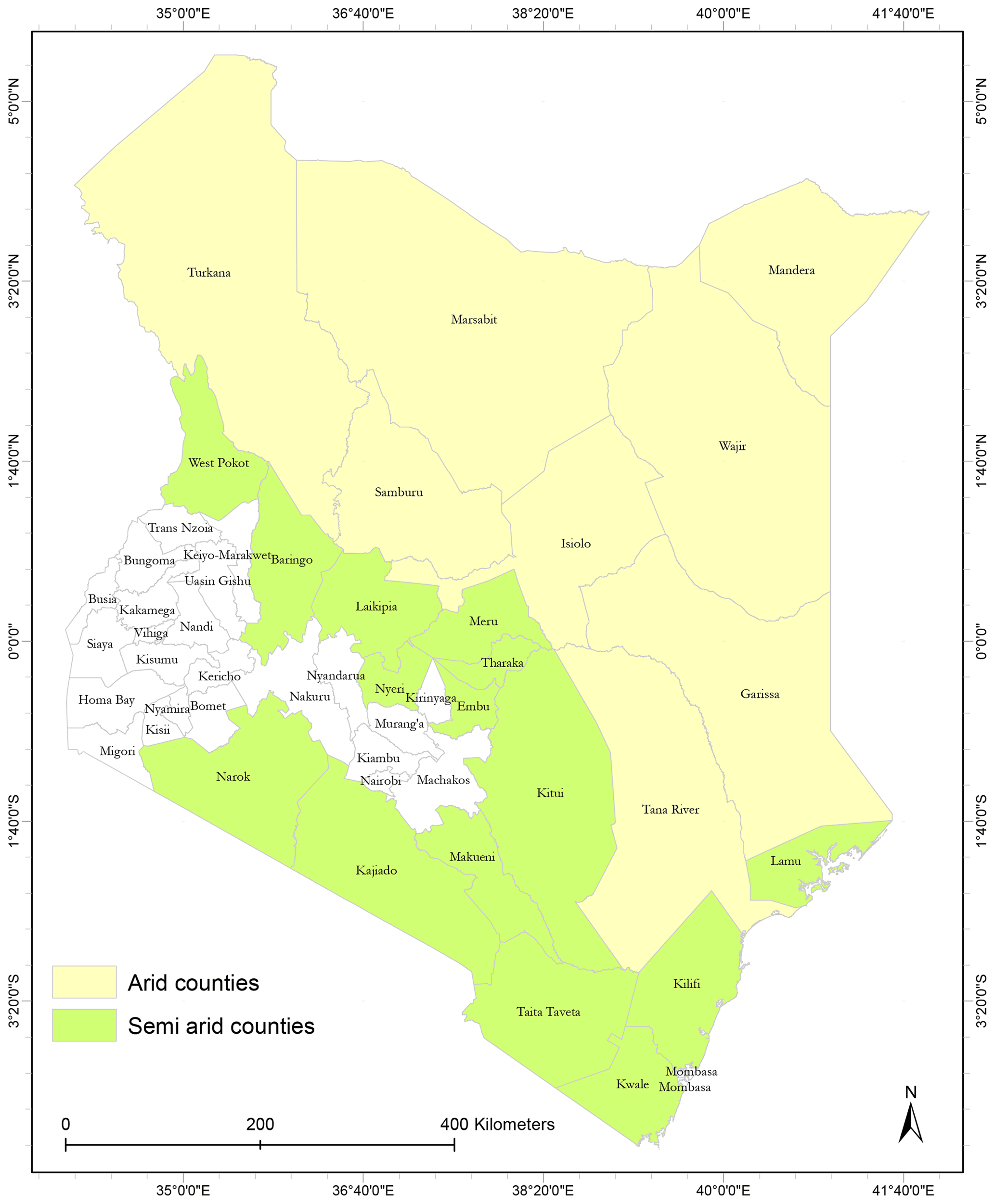
Figure 1A map of Kenya showing the arid and semi-arid counties where the research was focused. Data were sampled from 8 arid and 12 semi-arid counties.
2.2 Data
Developing a highly skilled model required adequate historical data on drought indicators and biophysical factors acquired over a long period. Table 1 shows details of the satellite earth observation data used for this work.
Table 1Summary of the datasets for the forecast model.
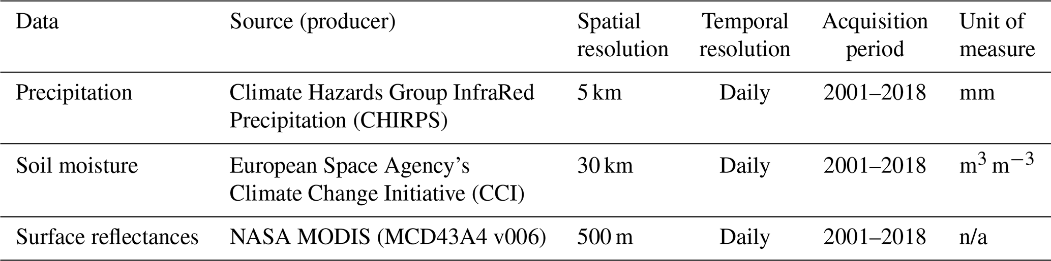
n/a means not applicable.
2.2.1 Precipitation (rainfall estimates)
The precipitation data were acquired from the Climate Hazards Group InfraRed Precipitation (CHIRPS) project (Funk et al., 2015). The CHIRPS data comprise a combination of weather station data and rainfall estimates captured via satellite remote sensing using the cold cloud duration (CCD) (Milford and Dugdale, 1990) approach. The approach is used to estimate rainfall by using remotely sensed information on the period of time a cloud remains at a given temperature. The dataset is available as daily 5 km resolution images.
2.2.2 Soil moisture
The daily 30 km resolution soil moisture products by the European Space Agency's Climate Change Initiative (ESA-CCI) were used for this work. The data are produced from an algorithm that takes in back-scatter information from multiple active and passive synthetic aperture radar (SAR) satellites. The values generated represent soil moisture at a soil depth of 10 cm. The ESA-CCI soil moisture products are available as passive, active, or a combination of both. For this work, the combined version of the data is used (Gruber et al., 2019; Dorigo et al., 2017; Yang et al., 2017).
2.2.3 Surface reflectance
The bidirectional reflectance distribution function (BRDF)-corrected MODIS product, MCD43A4 Version 6 (Schaaf and Wang, 2015), was used to compute the NDVI and VCI. The product is available as daily 500 m resolution images captured in seven bands ranging from visible to infrared. Information on the vegetation health is derived from the red and near-infrared (NIR) bands via Eq. (1).
3.1 Data pre-processing
The datasets were acquired from 1 January 2001 to 31 December 2018 to correspond with the availability of soil moisture data at the time of research. Apart from the precipitation, clouded and low-quality pixels from poor atmospheric and radiometric correction were removed using the quality flags from the quality assurance (QA) maps that came with the surface reflectance and soil moisture products. Pixels representing grassland and shrubland areas within our regions of interest were retrieved with the European Space Agency (ESA)'s 2016 Sentinel 2 land use and land Cover (LULC) map1 (Ramoino et al., 2018). For the coastal semi-arid counties like Lamu and Kwale we could not extract enough soil moisture data, so no results are shown for these counties.
To measure the drought condition at a period in time, the minimum and maximum NDVI values for a chosen baseline time interval and the NDVI value for that period are used to compute the vegetation condition index (VCI) via Eq. (2) (Kogan, 1995). VCI values range from 0–100, with values below 35 depicting a moderate to severe drought condition (Klisch and Atzberger, 2016).
where VCIi is the VCI value to be derived for the ith week, the NDVIi is the NDVI values for ith week, and NDVImin,i and NDVImax,i are the long-term minimum and long-term maximum NDVI values of a pixel for the ith week of the year.
The percentage of temporal gaps created by the removal of clouded and poor-quality pixels varied per county and ranged from as low as 0.1 % to 35 %. Counties with over 50 % missing data were dropped. Gaps were filled with the radial basis function (RBF) interpolation method. This approach uses weighted basis functions derived from Euclidean distances to approximate missing values (Rippa, 1999). The advantage of using the RBF method was to ensure approximated values did not fall outside the valid ranges, especially over periods with long gaps. Noise resulting from faulty instruments was reduced with the Whittaker smoother (Eilers, 2003), which filters noise via a penalised least squares. The gap filling and smoothing processes did not have any significant impact on the forecast model as shown in Barrett et al. (2020). Since our target variable was computed from the long-term minimum and maximum NDVI, the additional variables were also converted to anomalies by subtracting their long-term means to produce soil moisture anomaly and precipitation anomaly. The persistence within individual variables was enhanced by computing with 3-month (12 weeks) rolling averages to derive 3-month VCI (VCI3M), 3-month precipitation (P3M), and 3-month soil moisture (SM3M). Finally, the precipitation and soil moisture data were standardised to eliminate any associated units of measurements and avoid the dominance of certain variables. This was done by subtracting their mean and dividing it by the standard deviation.
3.2 Drought model and forecasting
The AR method used in Barrett et al. (2020) was used as a baseline model for this study. The AR(q) model, with q being the number of lags, used historical values of VCI3M in the linear regression model to forecast future VCI3M. The AR(q) model was defined as
where the Dt+n is the VCI3M at n lead time ahead, and Dt−q represents the lags (0 to q=3) of past VCI3M values. α0 represents the intercept and ϵt−p the error term.
The results from the AR baseline model were compared to the output of the auto-regressive distributed lag (ARDL) proposed in this paper. The ARDL modelling approach used for this work is a generalised form of the AR method mainly used for multivariate time series analysis. The method enables the variable of interest (dependent variable) to be modelled as a function of its lags and that of additional explanatory variables (independent variable) (Gujarati, 2003). An ARDL (p, q) consists of p, which represents the number of lags of the independent variable, and q, which is the auto-regressive part of the model, represents the number of lags of the dependent variable. This approach has been extensively used in the field of economics and modelling the effect of climate and environmental variables on vegetation (Lei and Peters, 2004; Ji and Peters, 2005).
For this study, however, parameter estimation for the ARDL was implemented within a Bayesian framework instead of using maximum likelihood methods based on ordinary least squares (OLS). The Bayesian framework enables the incorporation of domain knowledge about the parameters through the use of informative priors. The model parameters, with this approach, are inferred using the Markov Chain Monte Carlo (MCMC) (Neal, 1993) sampling algorithm. The sampling process generates posterior probability distribution of the model parameters. As a consequence, we get a full probability distribution of forecast values for all lead times, which makes it easy to quantify forecast uncertainty for making informed decisions (Martin, 2018; Lambert, 2018).
The MCMC is a well-established sampling algorithm used for parameter inference in Bayesian models. However, Asaad and Magadia (2019) outlined some of its limitations and recommended the use of the Hamiltonian Monte Carlo (HMC) (Hoffman and Gelman, 2014), an improved variant of the traditional MCMC algorithm which is based on Hamiltonian dynamics and converges faster to a global minimum for models with high-dimensional parameter space (Robert et al., 2018). Parameter inference for this work was done with the No-U-Turn Sampler (NUTS) (Hoffman and Gelman, 2014) version of HMC implemented with the PyMC3 (Salvatier et al., 2016) Python package.
The Bayesian ARDL model was used for forecasting VCI3M with lagged P3M, and S3M is defined as
where Dt+n is the drought index at n lead time, and Dt−q represents the lags (0 to q) of the drought indicator (dependent variable). Pt−p and St−p represent the lags 0 to p for precipitation and soil moisture, respectively. α0 is a constant representing the intercept, and βd, θp, and δs are the regression coefficients of the input variables with ϵt−p being the error term, which is assumed to be Gaussian.
Equation (4) can be re-written as
where n is the lead time, βi is the model parameters, and Xt−i represents the lagged input variables in Eq. (4).
The Bayesian approach makes explicit the prior beliefs about model parameters, which are then updated given some new data via the likelihood function, to give the posterior probability distribution.
Parameter inference with the Bayesian framework is based on Bayes' theorem via the equation below:
where θ is the model parameter; Xt represents Dt−q, Pt−p, and St−p; P(θ|Xt) is the posterior or the probability of our model parameters given our data Xt; P(Xt|θ) is the likelihood or the probability of the data given the parameters; and P(θ) is our prior belief about the parameters. P(Xt), known as the evidence, is a normalisation term that represents the probability of the data. The term is intractable and usually ignored (Lambert, 2018; McElreath, 2016). Thus Eq. (6) for Bayes' theorem is re-written as
To put the ARDL model (Eq. 5) in the context of Eq. (7), the likelihood function P(Xt|θ) is written as
Computing Eq. (7) requires very complex integrals (Lambert, 2018); thus the HMC sampling algorithm (Hoffman and Gelman, 2014) was used for estimating the model parameters.
The prior P(θ) for the model's regression coefficients are assumed to be Gaussian , with μ set to 0 to allow inferred parameters to have both positive and negative values and a weakly informative σ of 0.5 as a regularisation prior. This was done to avoid the approximation of unreasonable parameters (Martin, 2018). The weakly informative σ of 0.5 was chosen after a grid search to select optimal parameters. A summary of the data pre-processing and modelling can be seen in Fig. 2.
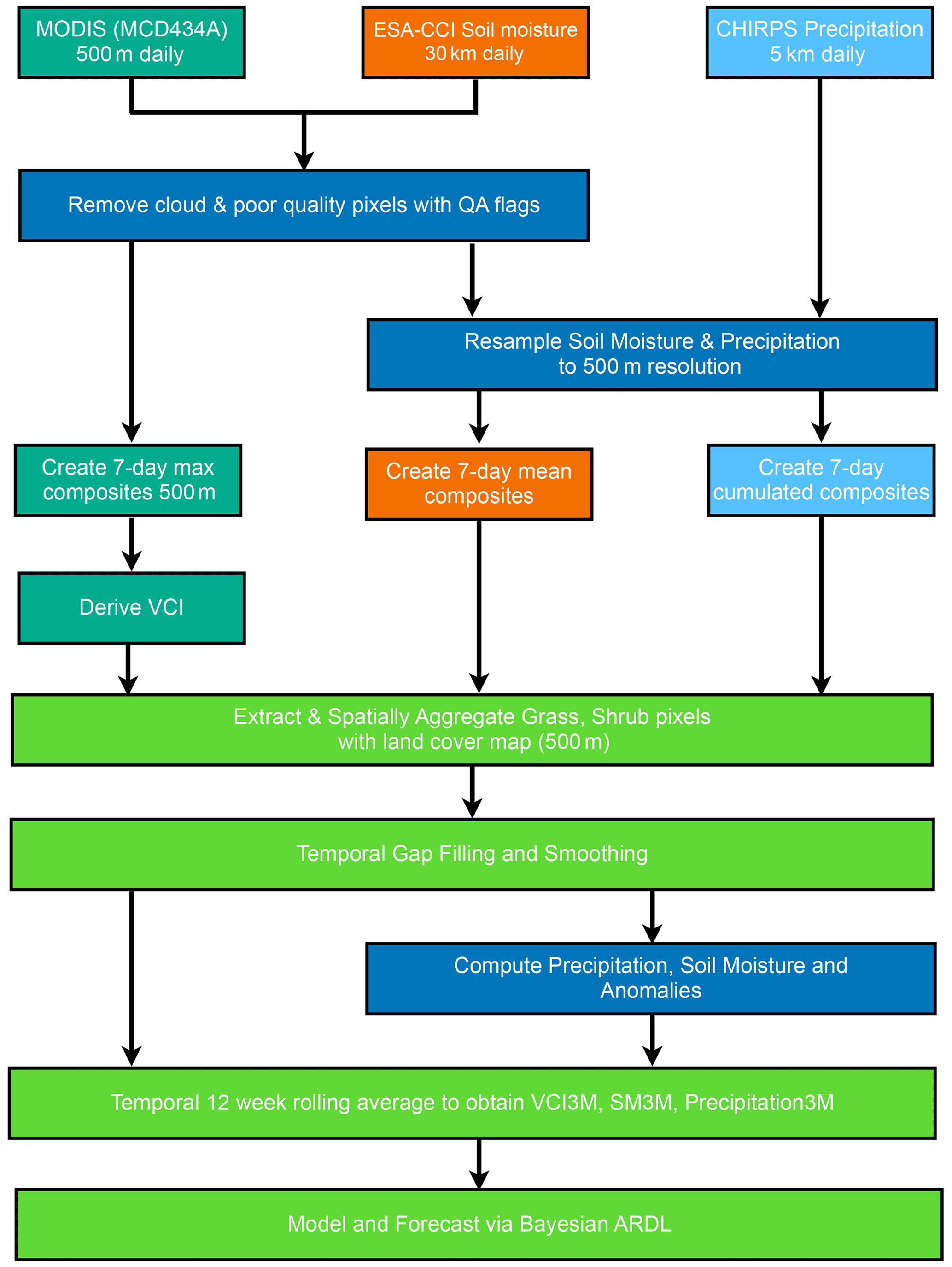
Figure 2A flow chart showing a summary of the data pre-processing and modelling steps detailed in Sects. 3 and 3.1.
3.3 Selecting optimal lags and forecasting
A full grid search was done with various combinations of p and q values for dependent and independent values to select the optimal p and q for the BARDL model. The Akaike information criterion (AIC) (Akaike, 1998) equation (Eq. 9) and the R2 (Eq. 10) metric were used as the score criteria to choose the optimal lags. AIC enables model selection by determining the model that best fits the data. The model with the lowest AIC value is preferred, whereas the R2 score explains how much variation in the observed data could be explained by the model. Valid R2 scores range between 0 and 1, where models with scores close to 1 are considered more accurate. The search was done on lag values ranging from 1 to 16 weeks. The best AIC and R2 scores varied for different lag combinations and also for each county. However, across all counties optimal AIC and R2 scores were obtained when all input variables were set to a lag of 6 weeks. The AIC scores are derived as follows:
where the RSS is the residual sum of squares error, n is the number of data points, and K is the number of estimated parameters.
The R2 scores are derived as follows:
where the yi is the observed data, is the mean of the observed data, and the fi is the forecasts.
Forecasting with the BARDL was done using the direct multi-step forecast approach, where separate models are fitted for n steps ahead of forecasts (Ben Taieb et al., 2010; Ben Taieb and Hyndman, 2014). To fit the model for n steps ahead, the data were restructured to offset values of the dependent (Dt+n), n weeks from lag 0 Xt−0, for all input variables. A rolling-window cross-validation approach (Hyndman and Athanasopoulos, 2018) was used for model training and forecasting. With this approach, the data are divided into chunks of 500 data points; for each chunk, 400 data points are used to train the model, and the remaining 100 data points are held out for prediction. The observed values from held-out data and mean forecast distribution from the Bayesian model were then used to evaluate the model skill.
3.4 Forecast skill assessment
The performance of the models was assessed by measuring the accuracy, i.e. how well the forecasts agree with the observations and the precision (the quoted uncertainty and the accuracy of that uncertainty).
The model accuracy was evaluated with the R2 (Eq. 10) and root mean square error (RMSE) (Eq. 11). The RMSE measures the mean deviation between the observed and forecast values.
where the yi is the observed data, fi is the forecasts, and n is the total number of data points.
The precision was quantified with the prediction interval coverage probability (PICP), and the mean prediction interval width (MPIW) (Pang et al., 2018) was also computed. The MPIW measures the average width between the upper (u(Di)) and lower bound l(Di) of a proportion of forecast distribution (n weeks ahead) defined by a chosen prediction interval (e.g. 95 %). See Fig. 3 for an illustration.
The PICP shows the percentage of time the observed variable lies within the credible interval of the forecast distribution and is derived as follows:
where N represents the number of predicted samples, and ci is either 0 or 1. If the observed drought target variable falls within the upper and lower bound of the forecast distribution (n weeks ahead) then ci=1; ci=0 (Fig. 3) if otherwise.

Figure 3A diagram illustrating how the prediction interval coverage probability (PICP) (a) and the mean prediction interval width (MPIW) (b) are computed.
The goal is to minimise the MPIW while maintaining a high PICP value. A high PICP value (0.90 to 0.99) indicates that the observed values lie within the forecast distribution, and a low MPIW value indicates a more precise forecast (Su et al., 2018). For the AR model, the confidence interval used to derive its PICP and MPIW was computed with the forecast RMSE and z score of 1.96, representing the 95 % confidence level of a standard normal distribution. This was done to permit its comparison to the output of the full BARDL model.
The contribution of the individual lagged input in the ARDL model was also measured by computing their percentage of relative importance via the relative weight analysis method (Tonidandel and LeBreton, 2011). With this approach, the input variables are initially transformed into orthogonal variables. Through an iterative process, each orthogonal variable is added to a linear regression model, and the change in R2 score for each iteration is measured and expressed as a percentage of the total R2 score.
The receiver operating characteristic (ROC) curve was also plotted to see how well the model forecasts a drought event given a threshold. The ROC shows the probability of a forecasted event being true (true positive rate – TPR) against the chance of that predicted event being a false alarm (false positive rate – FPR) at different thresholds. The area under the curve (AUC) quantifies the ability of the forecast model to distinguish between drought events (Wilks, 2006; Bradley, 1997).
The forecast distribution from our BARDL model enabled the computation of forecast probabilities given some drought thresholds. The forecast probability of a drought event was computed from the full forecast distribution from our posterior at a drought threshold of VCI < 35. The model's skill at accurately forecasting these probabilities was assessed by plotting and analysing a reliability diagram and sharpness. The reliability diagrams were plotted by using the same threshold of VCI < 35 to initially convert observed VCI3M data at a lead time into binary events, where 0 indicates a “no drought” and 1 indicates a “drought” event. The forecast probabilities and observed binaries were binned into standard intervals and plotted as a joint distribution of forecast probabilities and the relative frequency of the true observed drought event (where observed binaries = 1). The sharpness plots, on the other hand, are histograms of drought occurrences in each probability bin.
The reliability diagram shows how well forecast probabilities for a given drought event agreed with its corresponding observed event, while the sharpness shows the frequency of a forecasted drought event. (WWRP, 2009; Wilks, 2006).
Table 2R2 scores (6- to 12-week lead times) for AR modelled with lags of VCI3M only and BARDL modelled with lags of VCI3M with precipitation (P3M) and soil moisture (SM3M) for arid and semi-arid counties. The mean R2 values in this table do not correspond to R2 values in Fig. 4 because Fig. 4 shows the overall scores for all counties, while the table shows the scores for the separate arid and semi-arid zones.

4.1 Forecast accuracy
The AR modelling approach had proved to be skilful for short-range (2- to 6-week lead time) VCI3M forecasts (Barrett et al., 2020). However, the goal of this study was to extend the forecast range beyond 6 weeks while maintaining high accuracy by using the BARDL model and considering the effect of exogenous factors like precipitation and soil moisture. The results shown in this section are for 6- to 12-week lead time for the BARDL models and with the AR modelling as a comparative baseline. All the evaluation metrics for the BARDL outputs were computed with the mean forecast distributions from our Bayesian models.
The contour plots in Fig. 4 show a joint distribution (scatterplot) of the observed VCI3M and forecasted VCI3M at 6, 8, 10, and 12 weeks for both AR and the BARDL models. The coloured contour lines represent the bins of the joint histograms, and for each plot, the correlation (r), RMSE, and R2 were computed. Overall, the results from the BARDL model showed a roughly 2-week gain in the performance metrics. For instance, the R2 score for the AR model at 6 weeks is equivalent to the R2 score at 8-week lead time for the BARDL models. This pattern can be seen across all forecast ranges for the RMSE as well.
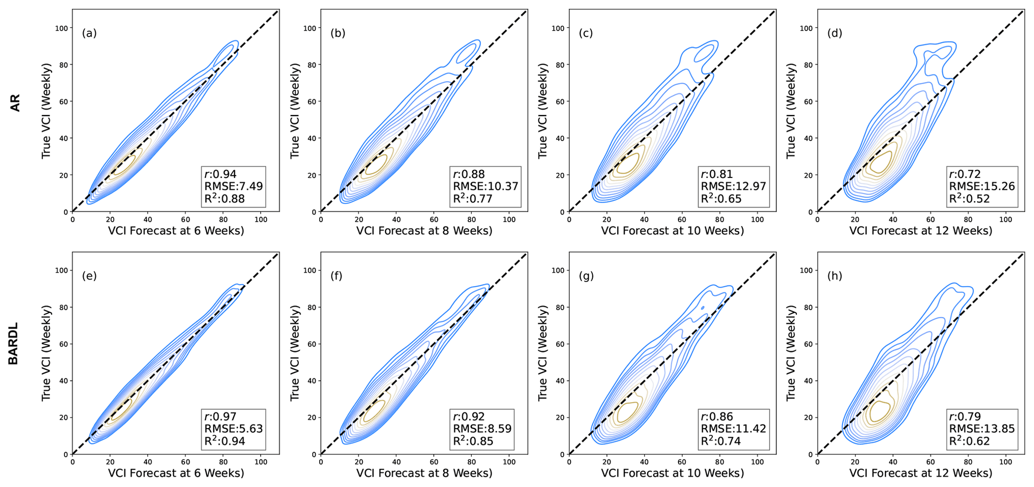
Figure 4Contour plots showing VCI3M forecast against true VCI3M. Panels (a)–(d) show the results from the AR method with VCI3M only, and panels (e)–(h) show the overall results for BARDL modelled with lags of VCI3M plus lags of precipitation (P3M) and soil moisture (S3M) anomalies for 6-, 8-, 10-, and 12-week lead time for all counties. The contour lines (ellipses) seen in each plot indicate the various bins that make up the joint histogram plots between the forecasted and observed VCI3M values. Contour lines with a yellow shade indicate values with stronger correlation between the observed and predicted values.
The performance metrics for the BARDL model in comparison to the AR model are shown in Fig. 5. This shows a significant improvement in performance at the same lead time, and, as a consequence, similar performance in the BARDL models is seen 2 weeks ahead of the AR models.
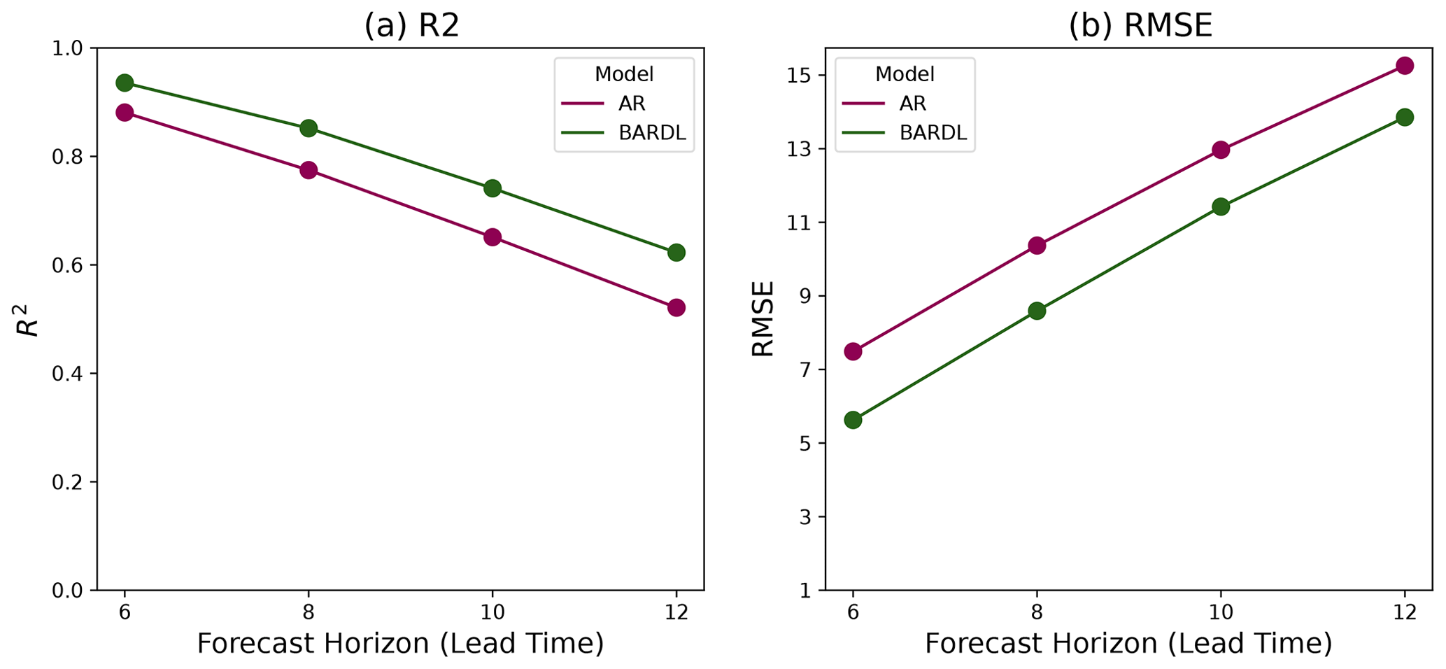
Figure 5Performance metrics used to measure model accuracy as a function of forecast lead time. R2 (a), RMSE (b).
Table 2 shows the R2 scores for 6- to 12-week forecasts for AR and BARDL models at the county level for arid and semi-arid regions. Just as observed in the contour plots, significant improvements are seen from 6- to 10-week lead time across all counties. In an arid county like Mandera, the R2 improved from 0.84, 0.72, and 0.58 using AR to 0.93, 0.84, and 0.73 using BARDL for 6-, 8-, and 10-week lead times, respectively. Kitui in the semi-arid region also showed an improvement in R2 score from 0.84, 0.71, and 0.57 to 0.91, 0.81, and 0.67 for weeks 6, 8, and 10, respectively. Overall the BARDL method demonstrated better results compared to the AR across all counties.
Further evaluation of forecasts based on Kenya's long rain (March, April, May – MAM) and short rain (October, November, December – OND) seasons (Camberlin and Wairoto, 1997) also showed even better R2 score for longer-range forecasting in the MAM season compared to the OND for the BARDL model as seen in Fig. 6 as well as in Fig. D1 in Appendix C.
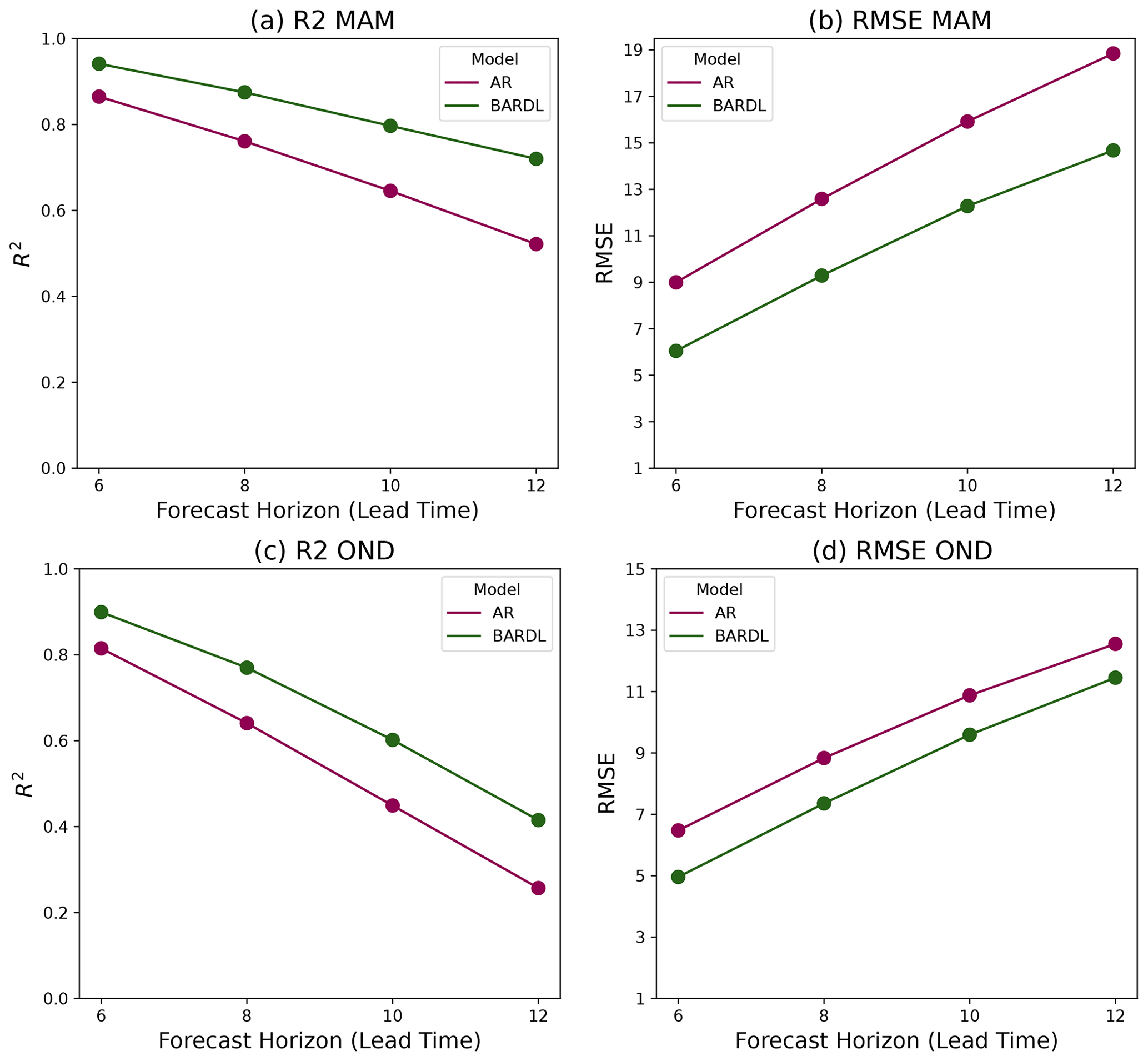
Figure 6Performance metrics used to measure model accuracy as a function of forecast lead time for MAM and OND season.
The R2 scores for the AR model in the MAM season however dropped significantly compared to the OND season.
4.2 Uncertainty analysis (PICP and MPIW)
The PICP and MPIW for a 95 % forecast confidence interval were computed for each lead time for both the AR and BARDL models. In Fig. 7, the time series plots show that the observed VCI3M values lie within the 95 % forecast interval between 90 %–94 % of the time across all lead times for both the BARDL and AR models. However, lower values of MPIW demonstrate that the BARDL provided more precise forecasts. Appendix A tabulates PICP and MPIW for 6- to 12-week forecasts for the AR and BARDL models for all counties (Table A1).
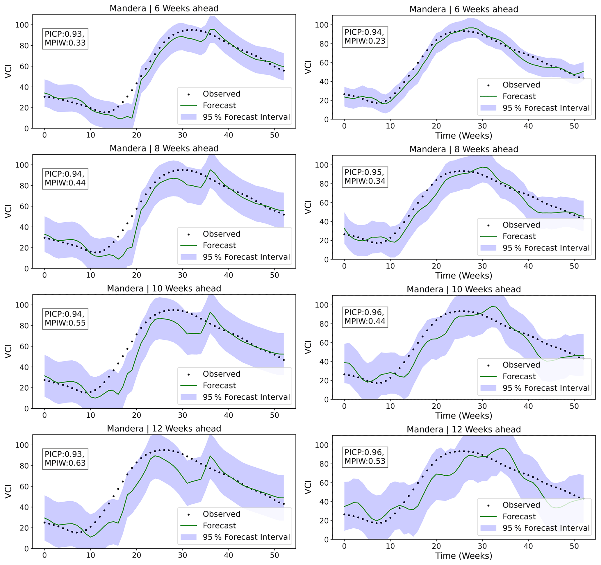
Figure 7Time series plot showing uncertainty for 6-, 8-, 10-, and 12-week lead time for Mandera County. Plots on the left side are from the AR model, and plots to the right are BARDL. The PICP and MPIW for the other counties can found in Appendix A. The forecast line (green line) represents the mean values of the BARDL outputs.
4.3 Drought event ROC curve
The receiver operating characteristic (ROC) curve (Fig. 8) illustrates how well the model can discriminate drought events. Drought events are forecasted when the predicted VCI3M drops below a threshold and are deemed correct if the observed VCI3M is below 35 (moderate to severe drought) (Klisch and Atzberger, 2016). The ROC curve and AUC metric for the BARDL model also demonstrated an improvement over the AR model. The points plotted on the curve represent the TPR and FPR where VCI3M < 35. This indicates that when the AR model (dotted curve) forecasts a drought condition (i.e. VCI3M < 35) for 6 weeks ahead, the probability of it being true is 86 % with a FPR of 9 %, whereas a forecast by the BARDL model (solid curve) at the same 6 weeks had a TPR of 89 % and a FPR of 7 %. The improvements with the BARDL model were mainly seen in the TPRs (6- to 10-week lead time) for the BARDL model, while the FPR remained almost the same. The improvements seen in the ROC curves in Fig. 8 are however not reflective of the distinct improvement seen in Fig. 5. The observed difference was because, whereas the R2 and RMSE are comparing the explained variances and deviation between the observed and forecast VCI3M, the ROC is mainly assessing the skill of both models at predicting drought occurrence at the VCI3M < 35 threshold.

Figure 8ROC curve showing true positive rate (TPR), false positive rate (FPR), and AUC for 6-, 8-, 10-, and 12-week lead time for both AR (dotted line) and BARDL (solid line) models. The VCI3M < 35 threshold is plotted as points on the lines. The AUC scores for models was above 80 %, indicating that both models were effective at identifying drought events.
4.4 Forecast reliability
Using the Bayesian approach also enabled the computation of forecast probabilities for a given drought event (no-drought condition: VCI3m > 35; drought condition: VCI3M < 35). To assess the skill for forecasting drought probabilities, we used the reliability diagrams in Fig. 9. The plot shows a joint distribution between the forecast probabilities in bins and the frequencies of the observed drought events that fall in those bins. For each lead time, the sharpness histogram, which shows the frequency at which an event is forecasted (WWRP, 2009), is also plotted. The reliability of a perfect model would follow the line y=x, which has been represented by a dashed line in Fig. 9. The closer a model is to this dashed line, the more reliable it is. Figure 9 shows the reliability for drought events (VCI3M < 35) in arid counties from the forecast skill assessment. Our BARDL model indicates that when we forecast a “drought event” with a probability between 80 % and 100 % for 6-week lead time, it corresponds with the observed drought events about 88 % to 99 % of the time. This diagram, however, showed that the forecast probabilities from the BARDL model do not always agree with the observed event, indicating a situation known as “under-forecasting” (Wilks, 2006).
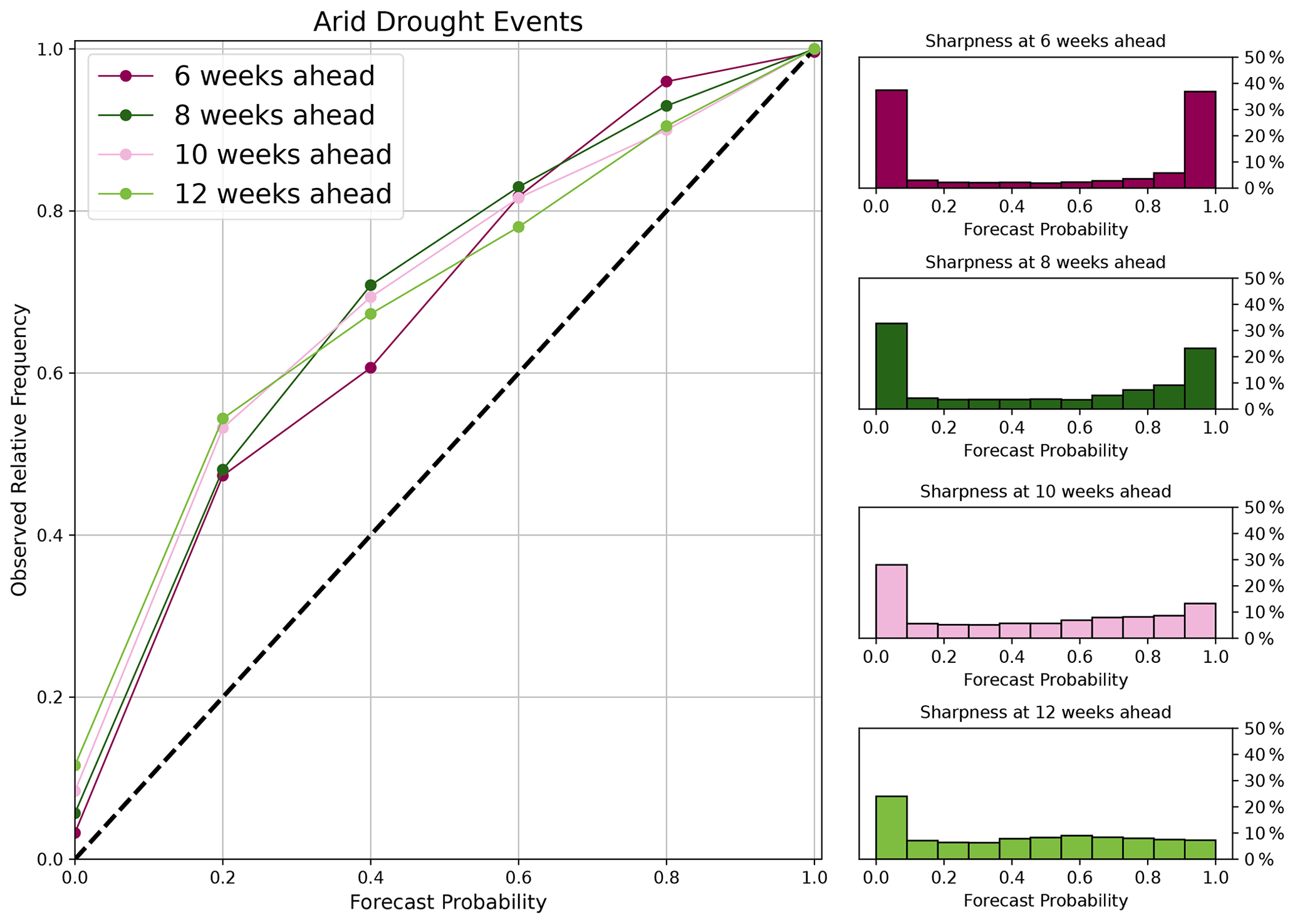
Figure 9Reliability diagram showing forecast probability and the corresponding observed frequencies for 6-, 8-, 10-, and 12-week lead time together with their corresponding sharpness plots for drought events (VCI3M < 35) in the arid and semi-arid counties.
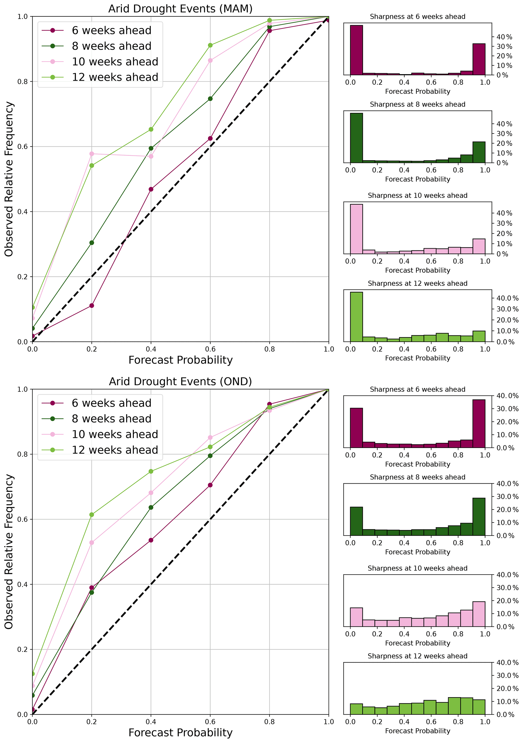
Figure 10Reliability diagram showing forecast probability and the corresponding observed frequencies for 6-, 8-, 10-, and 12-week lead time together with their corresponding sharpness plots for drought events (VCI3M < 35) in MAM and OND.
In terms of the model's sharpness, it can be seen that most of the drought events forecasted by the BARDL model have a probability between 90 % 100 %. The peak at the 0 % to 10 % bin of the sharpness plot shows the frequency of “no drought” forecasts in the arid counties. This indicates the likelihood of the model missing some drought events, especially from 8-week lead time and beyond.
Another key observation of the reliability diagrams for the MAM and OND seasons (Fig. 10) showed that the model was sharp at identifying more drought events in the short-rain season compared to the long-rain season.
4.5 Relative importance
Figure 11 shows the cumulative percentage of relative importance for the lags of VCI3M, P3M anomaly, and SM3M anomaly. The lags of VCI3M contribute the most for shorter lead time and decrease longer lead times. The precipitation anomaly also contributes significantly to future VCI3M, and its relative importance increases with increasing forecast lead times. The relative importance of soil moisture, although it varies less across various lead times, also contributes significantly. Detailed plots of the relative importance for individual lag contribution for each arid and semi-arid county are shown in Fig. B1 (Appendix B). Figure B1 also shows that input variables contributed mostly at lag 0. A critical look at these plots also shows that VCI3M responds better to precipitation anomaly in most arid counties like Turkana and Wajir compared to semi-arid counties like Kitui and West Pokot. The relative importance of the lagged exogenous factors for different MAM and OND seasons also confirms the reliance of future VCI3M on precipitation anomalies as seen Fig. C1 in Appendix D.
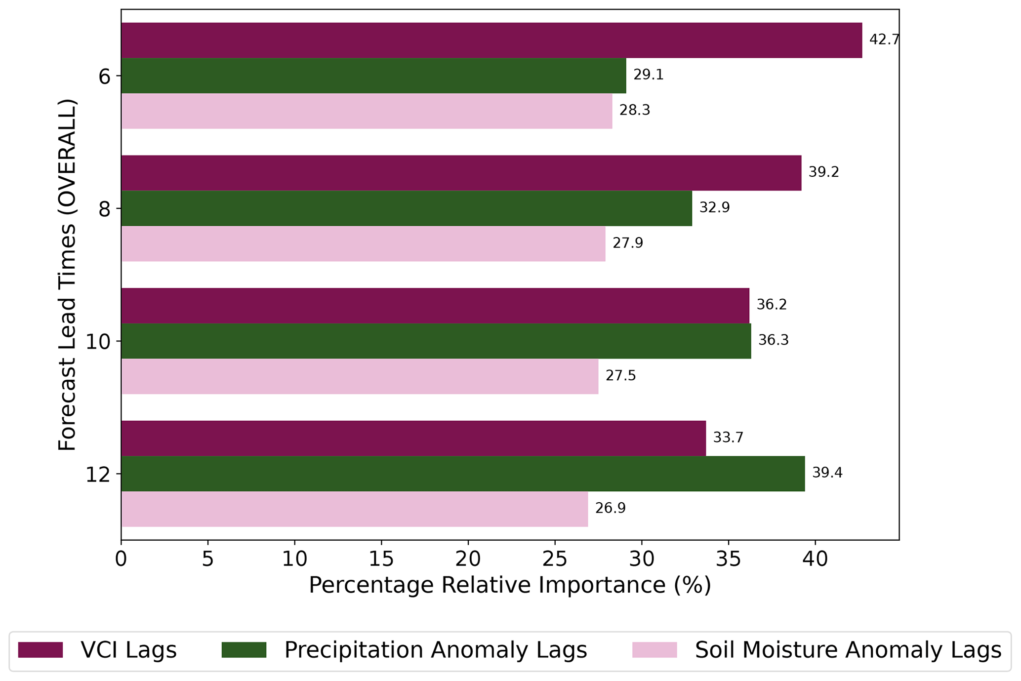
Figure 11Bar plots showing the cumulative (all lags) relative importance of additional variables to the VCI3M forecast for all counties.
Our BARDL model, which incorporated lagged precipitation and soil moisture anomalies as exogenous factors, exhibited an approximately 2-week gain in forecast range compared to the baseline model. These gains can be seen in Fig. 5 and Table 2, where, for instance, an R2 score obtained at a 6-week forecast for the AR model was equivalent to an R2 score at 8 weeks for the BARDL model. Forecasts from the BARDL were mostly driven by the variables at lag 0 (see Fig. B1). However, the collective contribution of the additional lags substantially improved the forecast ranges. Finally, the skill assessment based on forecast probabilities indicated a good separation between no-drought and drought events.
The results from the model evaluation revealed a strong persistence within soil moisture and VCI3M, a property that enables future values to be inferred from their past values (AghaKouchak, 2014). These could be seen from the lag contribution of soil moisture and precipitation in Figs. 11, B1, and C1. Despite this inherent persistence in the VCI3M, it still required the information from additional biophysical factors to improve its forecast range, as seen in Fig. B1 and the overall performance of the BARDL model. Another interesting observation from Fig. 11 also showed that VCI3M responded very slowly to short-term moisture anomalies (Quiring and Ganesh, 2010; Vicente-Serrano, 2007). From a spatial perspective, both models (AR and BARDL) gave a higher forecast R2 score in the arid areas compared to the semi-arid areas. This was more significant for the BARDL model.
The performance (R2 scores) of the BARDL model during the long rain (MAM) seasons indicated that although VCI3M responds slowly to short-term moisture levels, the impact of precipitation and soil moisture on vegetation condition is very vital. However the low R2 scores seen for the AR model in the MAM season could be attributed to the absence of information from the moisture levels (precipitation and soil moisture) in the AR model. The reliability plots for the MAM and OND seasons also showed that the contribution of the lagged soil moisture anomalies during the OND seasons also increased compared to the MAM season. This was an indication that during the short rain season, vegetation condition is controlled mostly by soil moisture. The sharpness plots in Fig. 9 also indicated that the model was generally sensitive to identifying drought events more frequently till 8 weeks ahead. However, when it comes to forecasting drought events, a much higher frequency is seen during the OND season (see Fig. 10). This is expected since there are fewer rainfalls in the OND seasons.
The uncertainty analysis from the PICP showed the observed VCI3M values were within the upper and lower bounds of the forecast distribution about 90 % of the time, indicating a low forecast uncertainty. The MPIW revealed that the forecast intervals were generally slightly narrower for the BARDL model compared to the AR model. Overall, higher PICP values were seen for AR; however, the PICP and MPIW values for the BARDL model are assumed to be a true representation of the forecast error since they were computed from forecast distribution.
Aside from the significant improvements in the forecast range and precision, the strength of our model hinges on the fact that we implemented it in a Bayesian context. Using the Bayesian approach generates a full posterior probability distribution of forecasted VCI3M values, which gave us the power to easily gain insight into the uncertainty in forecasted VCI3M values (Lambert, 2018). It also allowed the computation of probabilistic forecasting of specific drought events (e.g. VCI3M falling in a particular range) (Wilks, 2006). For our target end-users and stakeholders like the NDMA, using the Bayesian model proposed in this paper as part of their EWSs will enable them to confidently report on drought events. Also, policymakers and administrators of disaster relief organisations based on the forecast-based finance initiatives (Coughlan de Perez et al., 2015) can make better decisions and prioritise which drought alarms to act on. This will help with the efficient management of funds. The soil moisture data though retrieved via a combination of remote sensing and a soil moisture model (Gruber et al., 2019) also proved useful for drought monitoring and forecasting. The extensive model skill assessments done here show that our Bayesian ARDL approach not only performs better compared to results from previous studies (Barrett et al., 2020), but also, the BARDL model, by design, provides additional uncertainty information for better decision-making.
Although we have shown that we can extend forecast ranges with the added variables, the limitations to the work include the availability of soil moisture data. The ESA CCI soil moisture products used in this paper are released annually and are also a year behind. Thus they cannot currently be used for producing real-time forecasts. Another limitation was the use of the 2016 ESA Sentinel 2 land cover map for sampling grassland and shrub pixels across an 18-year period. Even though the land cover product accurately depicted areas with grassland and shrubs, pixel values from regions with significant land cover changes over time may be misleading.
In this paper we increase the range of VCI3M forecasts, using additional lagged information from P3M and S3M anomalies. The VCI3M used here was derived from the 12-week rolling mean of VCI, as used by Kenya's NDMA for monitoring and reporting agricultural drought occurrences. Key highlights in this paper include the improvement in the forecast range of VCI3M by approximately 2 weeks compared to the AR model used in our previous work. The improvement is attributed to lagged information from precipitation (P3M) and soil moisture (S3M). Secondly, modelling within the Bayesian framework also gave the added advantage of easily assessing model uncertainty and probability of a drought event. Results showed that our proposed model forecasted VCI3M at higher accuracy at a longer range during the MAM season and was also more sensitive to drought events during the OND season.
The forecast-based finance initiatives aimed at monitoring agricultural drought indicators and their impact on livelihoods should consider Bayesian approaches to enable better decision-making. We would also recommend that soil moisture data be made available sooner and promptly to enable near-real-time forecasting of vegetation condition via our proposed method.
The disparity in model performance between arid and semi-arid regions points to the fact that the differences in climate and vegetation land use and land cover (LULC) should also be considered when developing such forecast models. A natural expansion of our BARDL model would be to simultaneously explore and model for spatial variations like LULC in a county or any region of interest via a hierarchical modelling approach. Doing this will give us the advantage of pooling information between spatial variations whilst still allowing flexibility between them. The full version of the paper forecasting VCI3M with a hierarchical model can be found in Salakpi et al. (2022a), which is part 2 to this paper.
Table A1The PICP and MPIW (in parentheses) estimates for all arid and semi-arid counties.
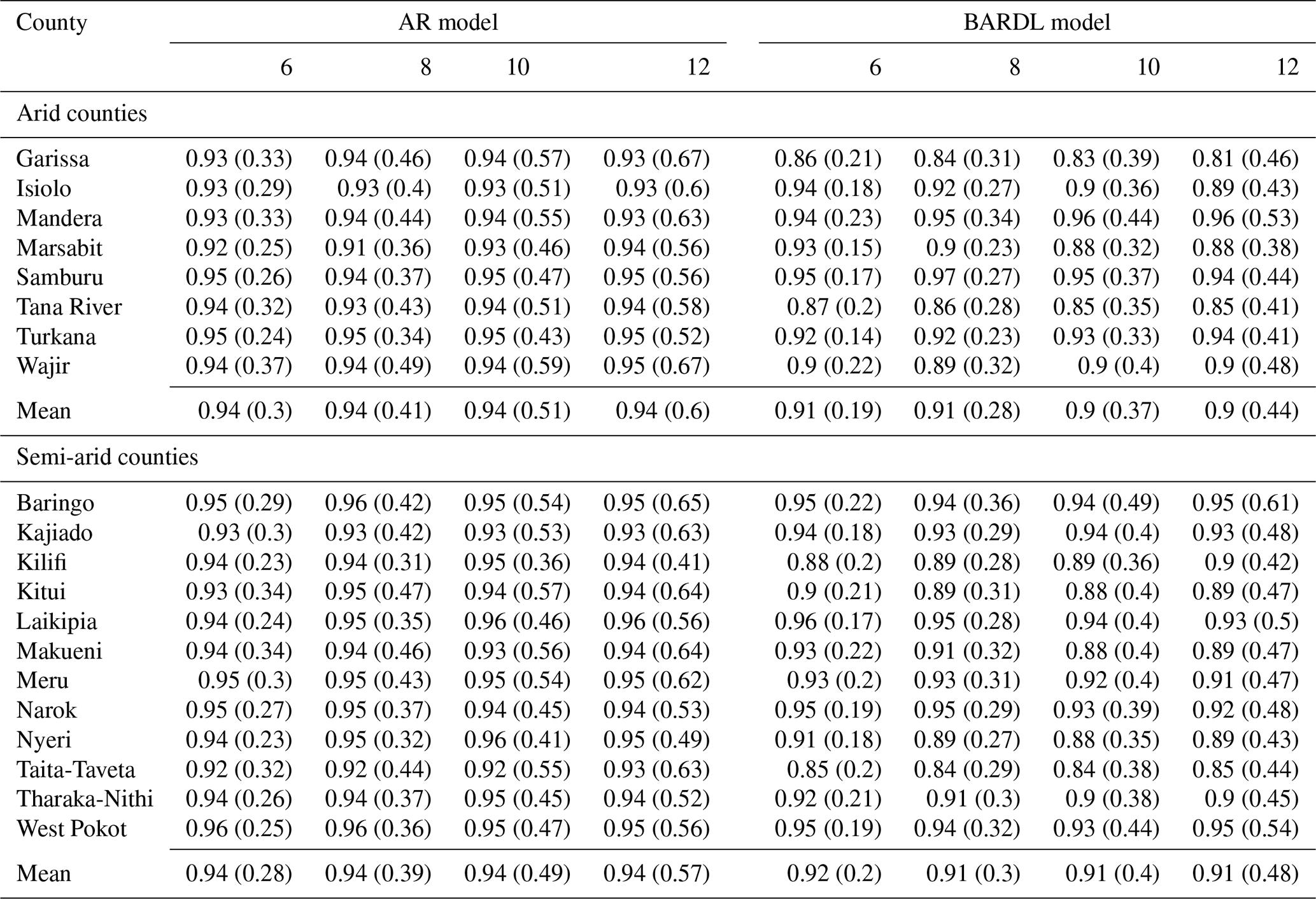
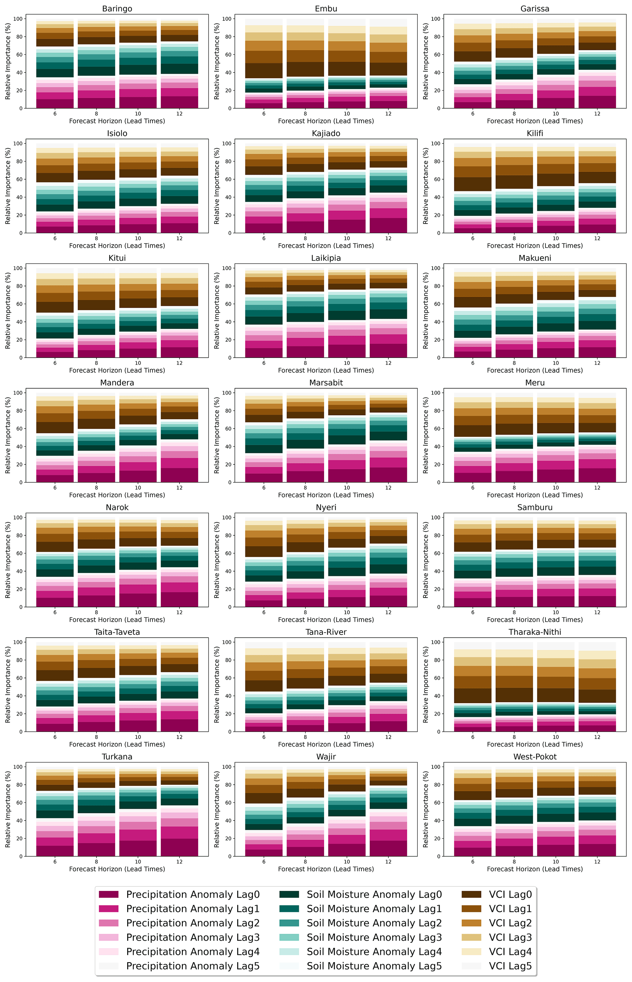
Figure B1Relative importance for each exogenous factor for each lag (0–5) variable per county. The distinct colour bands show the overall contribution of each input variable, while the varying shades within each band show the individual contribution of each lagged input variable of precipitation, soil moisture, and VCI.

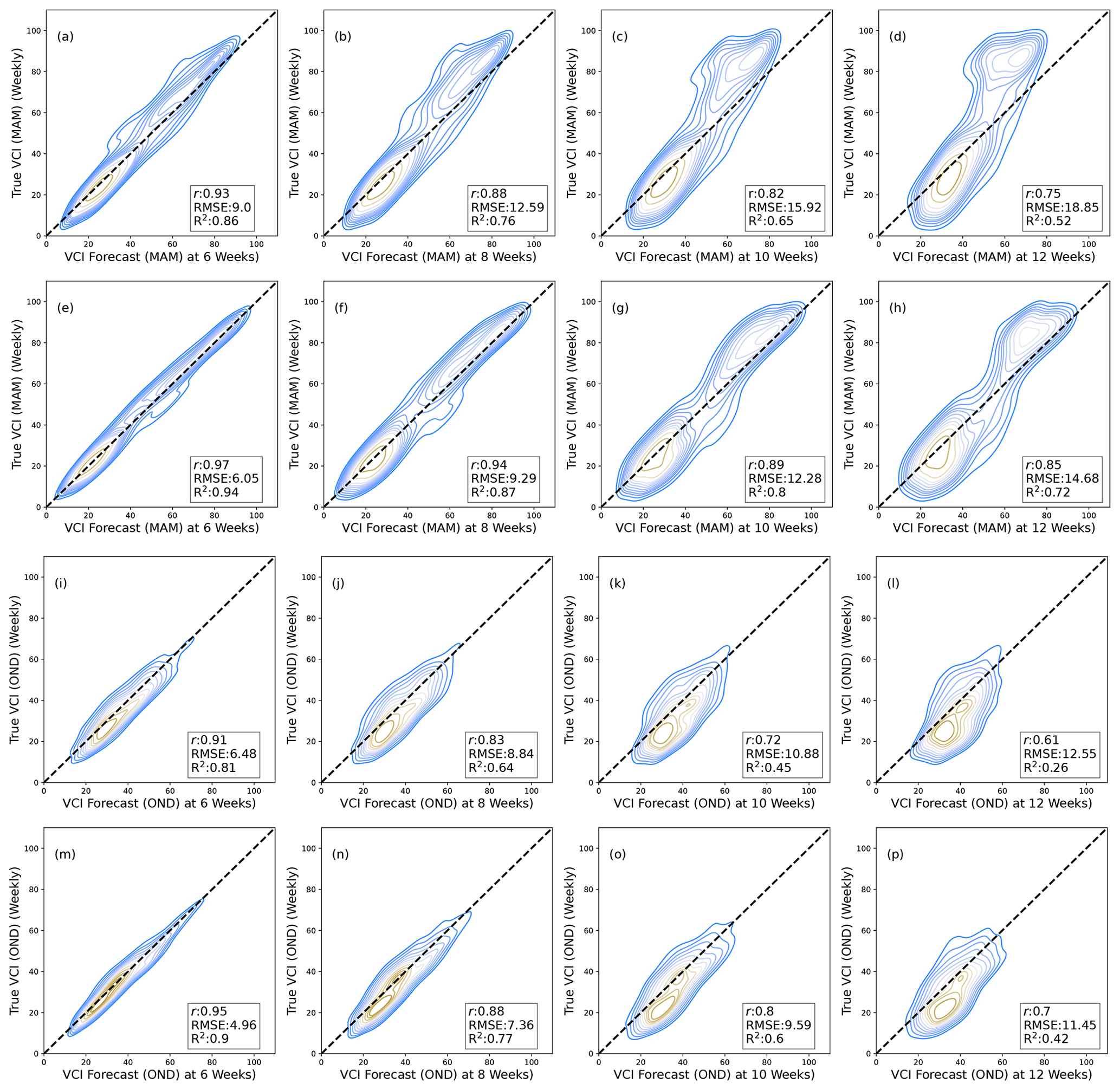
Figure D1Contour plots showing VCI3M forecast against true VCI3M for MAM and OND seasons. Panels (a)–(d) show the results from the AR method with VCI3M only, and (e)–(h) show the overall results for BARDL modelled with lags of VCI3M plus lags of precipitation (P3M) and soil moisture (S3M) anomalies for 6-, 8-, 10-, and 12-week lead time for all counties.
The data and code repository can be found here: https://doi.org/10.5281/zenodo.7005168 (Salakpi et al., 2022b).
EES is lead author and was responsible for data pre-processing, coding, modelling, and running the BARDL. JMM assisted with data acquisition, pre-processing, cartography, and feedback. ABB developed the code for the AR method. AB developed the code for the smoothing algorithm used for the time series data. SO, PR, and PH conceptualised the initial idea and provided supervision and feedback. The final paper was edited and reviewed by all authors.
The contact author has declared that none of the authors has any competing interests.
Publisher's note: Copernicus Publications remains neutral with regard to jurisdictional claims in published maps and institutional affiliations.
The work was funded by the UK Newton Fund's Development in Africa with Radio Astronomy (DARA) Big Data project delivered via STFC with grant number ST/R001898/1 and by the Science for Humanitarian Emergencies and Resilience (SHEAR) consortium project “Towards Forecast-based Preparedness Action” (ForPAc; https://sites.google.com/view/forpac-shear/home, last access: 21 July 2021), grant number NE/P000673/1, funded by the UK Natural Environment Research Council (NERC), the Economic and Social Research Council (ESRC), and the UK Department for International Development (DfID).
This research has been supported by the Newton Fund (grant no. ST/R001898/1), the UK Natural Environment Research Council (NERC), the Economic and Social Research Council (ESRC), and the UK Department for International Development (DfID) (grant no. NE/P000673/1).
This paper was edited by Maria-Carmen Llasat and reviewed by two anonymous referees.
Adede, C., Oboko, R., Wagacha, P. W., and Atzberger, C.: A Mixed Model Approach to Vegetation Condition Prediction Using Artificial Neural Networks (ANN): Case of Kenya's Operational Drought Monitoring, Remote Sens., 11, 1099, https://doi.org/10.3390/rs11091099, 2019. a
AghaKouchak, A.: A baseline probabilistic drought forecasting framework using standardized soil moisture index: Application to the 2012 United States drought, Hydrol. Earth Syst. Sci., 18, 2485–2492, https://doi.org/10.5194/hess-18-2485-2014, 2014. a, b
Akaike, H.: Information theory and an extension of the maximum likelihood principle, in: Selected papers of hirotugu akaike, Springer, New York, NY, 199–213, https://doi.org/10.1007/978-1-4612-1694-0_15, 1998. a
Asaad, A.-A. B. and Magadia, J. C.: Stochastic Gradient Hamiltonian Monte Carlo on Bayesian Time Series Modeling, in: 14th National Convention on Statistics Crowne Plaza Manila Galleria, 1–3 October 2019, Ortigas Center, Quezon City, 2019. a
Barrett, A. B., Duivenvoorden, S., Salakpi, E. E., Muthoka, J. M., Mwangi, J., Oliver, S., and Rowhani, P.: Forecasting vegetation condition for drought early warning systems in pastoral communities in Kenya, Remote Sens. Environ., 248, 111886, https://doi.org/10.1016/j.rse.2020.111886, 2020. a, b, c, d, e
Ben Taieb, S. and Hyndman, R. J.: Recursive and direct multi-step forecasting: the best of both worlds, in: International Journal of Forecasting, https://citeseerx.ist.psu.edu/viewdoc/download?doi=10.1.1.375.7885&rep=rep1&type=pdf (last access: 14 August 2022), 2014. a
Ben Taieb, S., Sorjamaa, A., and Bontempi, G.: Multiple-output modeling for multi-step-ahead time series forecasting, Neurocomputing, 73, 1950–1957, https://doi.org/10.1016/j.neucom.2009.11.030, 2010. a
Bowell, A., Salakpi, E. E., Guigma, K., Muthoka, J. M., Mwangi, J., and Rowhani, P.: Validating commonly used drought indicators in Kenya, Environ. Res. Lett., 16, 084066, https://doi.org/10.1088/1748-9326/ac16a2, 2021. a
Bradley, A. P.: The use of the area under the ROC curve in the evaluation of machine learning algorithms, Pattern Recognit., 30, 1145–1159, https://doi.org/10.1016/S0031-3203(96)00142-2, 1997. a
Cabot Venton, C., Fitzgibbon, C., Shitarek, T., Coulter, L., and Dooley, O.: Economics of Resilience Final Report The Economics of Early Response and Disaster Resilience: Lessons from Kenya and Ethiopia, Tech. rep., https://assets.publishing.service.gov.uk/media/57a08a63e5274a27b200058f/61114_Kenya_Report.pdf (last access: 21 July 2021), 2012. a
Camberlin, P. and Wairoto, J. G.: Intraseasonal wind anomalies related to wet and dry spells during the “long”and “short”rainy seasons in Kenya, Theor. Appl. Climatol., 58, 57–69, https://doi.org/10.1007/BF00867432, 1997. a
Cenacchi, N.: Drought risk reduction in agriculture: A review of adaptive strategies in East Africa and the Indo-Gangetic plain of South Asia, IFPRI Discussion Paper 1372, IFPRI – International Food Policy Research Institute, Washington, DC, https://ebrary.ifpri.org/utils/getfile/collection/p15738coll2/id/128277/filename/128488.pdf (last access: 21 July 2021), 2014. a
Coughlan de Perez, E., van den Hurk, B., van Aalst, M. K., Jongman, B., Klose, T., and Suarez, P.: Forecast-based financing: an approach for catalyzing humanitarian action based on extreme weather and climate forecasts, Nat. Hazards Earth Syst. Sci., 15, 895–904, https://doi.org/10.5194/nhess-15-895-2015, 2015. a
Deleersnyder, R.: Pastoralism in East Africa: challenges and solutions | Glo.be, https://www.glo-be.be/index.php/en/articles/pastoralism-east-africa-challenges-and-solutions (last access: 21 July 2021), 2018. a
Dorigo, W., Wagner, W., Albergel, C., Albrecht, F., Balsamo, G., Brocca, L., Chung, D., Ertl, M., Forkel, M., Gruber, A., Haas, E., Hamer, P. D., Hirschi, M., Ikonen, J., de Jeu, R., Kidd, R., Lahoz, W., Liu, Y. Y., Miralles, D., Mistelbauer, T., Nicolai-Shaw, N., Parinussa, R., Pratola, C., Reimer, C., van der Schalie, R., Seneviratne, S. I., Smolander, T., and Lecomte, P.: ESA CCI Soil Moisture for improved Earth system understanding: State-of-the art and future directions, Remote Sens. Environ., 203, 185–215, https://doi.org/10.1016/j.rse.2017.07.001, 2017. a
Eilers, P. H. C.: A Perfect Smoother, Anal. Chem., 75, 3631–3636, https://doi.org/10.1021/ac034173t, 2003. a
FAO: Easing the impact of drought in Kenya: FAO in Emergencies, http://www.fao.org/emergencies/resources/photos/photo-detail/en/c/1053828/ (last access: 21 July 2021), 2017. a
FAO: Pastoralism in Africa's drylands Reducing risks, addressing vulnerability and enhancing resilience, Tech. rep., http://www.fao.org/3/ca1312en/CA1312EN.pdf (last access: 21 July 2021), 2018. a, b
FEWSNET: Famine Early Warning Systems Network, FEWS NET, https://fews.net/ (last access: 21 July 2021), 2019. a
Funk, C., Peterson, P., Landsfeld, M., Pedreros, D., Verdin, J., Shukla, S., Husak, G., Rowland, J., Harrison, L., Hoell, A., and Michaelsen, J.: The climate hazards infrared precipitation with stations – A new environmental record for monitoring extremes, Scient. Data, 2, 1–21, https://doi.org/10.1038/sdata.2015.66, 2015. a
Gebremeskel, G., Tang, Q., Sun, S., Huang, Z., Zhang, X., and Liu, X.: Droughts in East Africa: Causes, impacts and resilience, Earth-Sci. Rev., 193, 146–161, https://doi.org/10.1016/j.earscirev.2019.04.015, 2019. a, b
Gruber, A., Scanlon, T., Van Der Schalie, R., Wagner, W., and Dorigo, W.: Evolution of the ESA CCI Soil Moisture climate data records and their underlying merging methodology, Earth Syst. Sci. Data, 11, 717–739, https://doi.org/10.5194/essd-11-717-2019, 2019. a, b
Gujarati, D.: Basic Econometrics, Economic series, McGraw Hill, https://books.google.co.uk/books?id=byu7AAAAIAAJ (last access: 21 July 2021), 2003. a, b
Han, P., Wang, P. X., Zhang, S. Y., and Zhu, D. H.: Drought forecasting based on the remote sensing data using ARIMA models, Math. Comput. Model., 51, 1398–1403, https://doi.org/10.1016/j.mcm.2009.10.031, 2010. a
Hoffman, M. D. and Gelman, A.: The no-U-turn sampler: Adaptively setting path lengths in Hamiltonian Monte Carlo, J. Mach. Learn. Res., 15, 1593–1623, 2014. a, b, c
Hyndman, R. J. and Athanasopoulos, G.: Forecasting: principles and practice, OTexts, USA, https://otexts.com/fpp2/ (last access: 21 July 2021), 2018. a
Jalili, M., Gharibshah, J., Ghavami, S. M., Beheshtifar, M., and Farshi, R.: Nationwide prediction of drought conditions in Iran based on remote sensing data, IEEE T. Comput., 63, 90–101, https://doi.org/10.1109/TC.2013.118, 2014. a
Ji, L. and Peters, A. J.: Lag and seasonality considerations in evaluating AVHRR NDVI response to precipitation, Photogram. Eng. Remote Sens., 71, 1053–1061, https://doi.org/10.14358/PERS.71.9.1053, 2005. a
Klisch, A. and Atzberger, C.: Operational drought monitoring in Kenya using MODIS NDVI time series, Remote Sens., 8, 267, https://doi.org/10.3390/rs8040267, 2016. a, b, c
Kogan, F. N.: Application of vegetation index and brightness temperature for drought detection, Adv. Space Res., 15, 91–100, https://doi.org/10.1016/0273-1177(95)00079-T, 1995. a
Lambert, B.: A Student's Guide to Bayesian Statistics, SAGE Publications, https://books.google.co.uk/books?id=ZvBUDwAAQBAJ (last acces: 21 July 2021), 2018. a, b, c, d, e
Lei, J. and Peters, A. J.: Forecasting vegetation greenness with satellite and climate data, IEEE Geosci. Remote Sens. Lett., 1, 3–6, https://doi.org/10.1109/LGRS.2003.821264, 2004. a
Marigi, S. N., Njogu, A. K., and Githungo, W. N.: Trends of Extreme Temperature and Rainfall Indices for Arid and Semi-Arid Lands of South Eastern Kenya, J. Geosci. Environ. Protect., 04, 158–171, https://doi.org/10.4236/gep.2016.412012, 2016. a
Martin, O.: Bayesian Analysis with Python: Introduction to statistical modeling and probabilistic programming using PyMC3 and ArviZ, 2nd Edn., Packt Publishing, https://books.google.co.uk/books?id=1Z2BDwAAQBAJ (last acces: 21 July 2021), 2018. a, b, c
McElreath, R.: Statistical Rethinking: A Bayesian Course with Examples in R and Stan, Chapman & Hall/CRC Texts in Statistical Science, CRC Press, https://books.google.co.uk/books?id=1yhFDwAAQBAJ (last acces: 21 July 2021), 2016. a
Milford, J. R. and Dugdale, G.: Monitoring of rainfall in relation to the control of migrant pests, Philos. T. Roy. Soc. Lond. B, 328, 689–704, https://doi.org/10.1098/rstb.1990.0137, 1990. a
Nay, J., Burchfield, E., and Gilligan, J.: A machine-learning approach to forecasting remotely sensed vegetation health, Int. J. Remote Sens., 39, 1800–1816, https://doi.org/10.1080/01431161.2017.1410296, 2018. a
Neal, R. M.: Probabilistic inference using Markov chain Monte Carlo methods, Department of Computer Science, University of Toronto Toronto, Ontario, Canada, 1993. a
Pang, J., Liu, D., Peng, Y., and Peng, X.: Optimize the coverage probability of prediction interval for anomaly detection of sensor-based monitoring series, Sensors (Switzerland), 18, 967, https://doi.org/10.3390/s18040967, 2018. a
Pesaran, M. H. and Shin, Y.: An Autoregressive Distributed-Lag Modelling Approach to Cointegration Analysis, in: Econometric Society Monographs, Cambridge University Press, 371–413, https://doi.org/10.1017/CCOL521633230.011, 1999. a
Quiring, S. M. and Ganesh, S.: Evaluating the utility of the Vegetation Condition Index (VCI) for monitoring meteorological drought in Texas, Agr. Forest Meteorol., 150, 330–339, https://doi.org/10.1016/j.agrformet.2009.11.015, 2010. a
Ramoino, F., Pera, F., and Arino, O.: `S2 prototype LC map at 20 m of Africa 2016' Users Feedback Compendium [6th February 2018], p. 12, http://due.esrin.esa.int/files/S2_prototype_LC_map_at_20m_of_Africa_2016-Users_Feedback_Compendium-6-Feb-2018.pdf (last access: 21 July 2021), 2018. a
Rippa, S.: An algorithm for selecting a good value for the parameter c in radial basis function interpolation, Adv. Comput. Math., 11, 193–210, https://doi.org/10.1023/A:1018975909870, 1999. a
Robert, C. P., Elvira, V., Tawn, N., and Wu, C.: Accelerating MCMC algorithms, Wiley Interdisciplin. Rev.: Comput. Stat., 10, e1435, https://doi.org/10.1002/WICS.1435, 2018. a
Salakpi, E. E., Hurley, P. D., Muthoka, J. M., Bowell, A., Oliver, S., and Rowhani, P.: A dynamic hierarchical Bayesian approach for forecasting vegetation condition, Nat. Hazards Earth Syst. Sci., 22, 2725–2749, https://doi.org/10.5194/nhess-22-2725-2022, 2022a. a
Salakpi, E. E., Barrett, A. B., and Bowell, A.: edd3x/Bayesian-ARDL: Data and Code for Bayesian Auto-regressive Distributed lag models (v.1.0), Zenodo [code], https://doi.org/10.5281/zenodo.7005168, 2022b. a
Salvatier, J., Wiecki, T. V., and Fonnesbeck, C.: Probabilistic programming in Python using PyMC3, Peer J. Comput. Sci., 2, e55, https://doi.org/10.7717/peerj-cs.55, 2016. a
Schaaf, C. and Wang, Z.: MCD43A4 MODIS/Terra+Aqua BRDF/Albedo Nadir BRDF Adjusted Ref Daily L3 Global – 500 m V006, USGS [data set], https://doi.org/10.5067/MODIS/MCD43A4.006, 2015. a
Sibanda, M., Mutanga, O., Rouget, M., and Kumar, L.: Estimating biomass of native grass grown under complex management treatments using worldview-3 spectral derivatives, Remote Sens., 9, 55, https://doi.org/10.3390/rs9010055, 2017. a
Su, D., Ting, Y. Y., and Ansel, J.: Tight Prediction Intervals Using Expanded Interval Minimization, http://arxiv.org/abs/1806.11222 (last access: 21 July 2021), 2018. a
Tian, M., Wang, P., and Khan, J.: Drought Forecasting with Vegetation Temperature Condition Index Using ARIMA Models in the Guanzhong Plain, Remote Sens., 8, 690, https://doi.org/10.3390/rs8090690, 2016. a
Tonidandel, S. and LeBreton, J. M.: Relative importance analysis: A useful supplement to regression analysis, J. Business Psychol., 26, 1–9, 2011. a
UNFCCC: Adoption of the Paris Agreement – Paris Agreement text English, Tech. rep., https://unfccc.int/sites/default/files/english_paris_agreement.pdf (last access: 21 July 2021), 2015. a
Vatter, J.: DROUGHT RISK The Global Thirst for Water in the Era of Climate Crisis, Tech. Rep., WWF – World Wildlife Fund, Germany, https://epoqstudio.com/ (last access: 21 July 2021), 2019. a
Vicente-Serrano, S. M.: Evaluating the impact of drought using remote sensing in a Mediterranean, Semi-arid Region, Nat. Hazards, 40, 173–208, https://doi.org/10.1007/s11069-006-0009-7, 2007. a
Vicente-Serrano, S. M., Beguería, S., Gimeno, L., Eklundh, L., Giuliani, G., Weston, D., Kenawy, A. E., López-Moreno, J. I., Nieto, R., Ayenew, T., Konte, D., Ardö, J., and Pegram, G. G.: Challenges for drought mitigation in Africa: The potential use of geospatial data and drought information systems, Appl. Geogr., 34, 471–486, https://doi.org/10.1016/j.apgeog.2012.02.001, 2012. a
Wilks, D.: Statistical methods in the atmospheric sciences, in: Vol. 100, Academic Press, ISBN 9780123850232, 0123850231, 2006. a, b, c, d
WWRP: World Weather Research Programme (WWRP), Forecast Verification – Methods and FAQ, https://www.cawcr.gov.au/projects/verification/verif_web_page.html (last access: 21 July 2021), 2009. a, b
Yang, Y., Xiao, P., Feng, X., and Li, H.: Accuracy assessment of seven global land cover datasets over China, ISPRS J. Photogram. Remote Sens., 125, 156–173, https://doi.org/10.1016/j.isprsjprs.2017.01.016, 2017. a
Yihdego, Y., Vaheddoost, B., and Al-Weshah, R. A.: Drought indices and indicators revisited, Arab. J. Geosci., 12, 1–12, https://doi.org/10.1007/S12517-019-4237-Z, 2019. a
Visit http://2016africalandcover20m.esrin.esa.int/ (last access: 21 July 2021) to learn more.
- Abstract
- Introduction
- Study area and data
- Methods
- Results
- Discussion
- Conclusion and future work
- Appendix A: A table showing the PICP and MPIW (in brackets) estimates for the arid and semi-arid counties
- Appendix B: Relative importance plots for each county
- Appendix C: Relative importance plots for MAM and OND seasons
- Appendix D: Contour plots showing forecast performance for MAM and OND seasons
- Code and data availability
- Author contributions
- Competing interests
- Disclaimer
- Acknowledgements
- Financial support
- Review statement
- References