the Creative Commons Attribution 4.0 License.
the Creative Commons Attribution 4.0 License.
 | 29 Aug 2024
Exploring the sensitivity of extreme event attribution of two recent extreme weather events in Sweden using long-running meteorological observations
Erik Kjellström
Despite a growing interest in extreme event attribution, attributing individual weather events remains difficult and uncertain. We have explored extreme event attribution by comparing the method for probabilistic extreme event attribution employed at World Weather Attribution (https://www.worldweatherattribution.org, last access: 22 August 2024) (WWA method) to an approach solely using pre-industrial and current observations (PI method), utilising the extensive and long-running network of meteorological observations available in Sweden. With the long observational records, the PI method is used to calculate the change in probability for two recent extreme events in Sweden without relying on the correlation to the global mean surface temperature (GMST). Our results indicate that the two methods generally agree for an event based on daily maximum temperatures. However, the WWA method results in a weaker indication of attribution compared to the PI method, for which 12 out of 15 stations indicate a stronger attribution than found by the WWA method. On the other hand, for a recent extreme precipitation event, the WWA method results in a stronger indication of attribution compared to the PI method. For this event, only 2 out of 10 stations assessed in the PI method exhibited results similar to the WWA method. Based on the results, we conclude that at least one out of every two of heat waves similar to the summer of 2018 can be attributed to climate change. For the extreme precipitation event in Gävle in 2021, the large variations within and between the two methods make it difficult to draw any conclusions regarding the attribution of the event.
- Article
(9346 KB) - Full-text XML
- BibTeX
- EndNote


Anthropogenic greenhouse gases were the main drivers of the observed increases in global temperatures during the 20th century (Eyring et al., 2021). Even though global warming is accompanied by a notable increase in the intensity and frequency of local extreme temperature and precipitation events (Trenberth, 2011; Seneviratne et al., 2021), linking individual extreme weather events to anthropogenic emissions remains a challenge.
Extreme weather events typically display unusual meteorological properties, have severe effects on society, and occur relatively infrequently. However, the frequency and intensity of many of today's extreme events are expected to change with the ongoing changes in the global climate. For extreme events such as hurricanes (Holland and Bruyère, 2014) and heat waves (Wilcke et al., 2020), changes in their climatology have already been observed. Furthermore, extreme weather, and its consequences have often already been experienced, which makes extreme weather particularly interesting to scientists as well as to the public in general. Hence, a question often asked is whether any specific especially intense weather event was caused by anthropogenic changes to the climate.
The relatively novel field of extreme event attribution (EEA) arose out of the need to try to answer questions like this. EEA is a collection of methods used to investigate whether an extreme event can be attributed to any one forcing, such as anthropogenic climate change (e.g. Stott et al., 2016; van Oldenborgh et al., 2021). The last decade has seen a rapid increase in both the number of publications of and general interest in EEA studies. A notable example is the BAMS special issue “Explaining Extreme Events” (e.g. Herring et al., 2022), which has been published annually since 2011. Olsson et al. (2022) argue that the increasing interest in EEA is connected to the ongoing development of the framework for loss and damage (L&D), where the attribution of single events could become a useful tool (Parker et al., 2015). The possible use of EEA in future L&D programmes, combined with the increasing societal interest in extreme weather events, makes the exploration and evaluation of the suggested methods both compelling and important.
There are several approaches to EEA, where two of the more common ones are the risk-based approach and the storyline approach. In the risk-based approach, as described in, for example, Stott et al. (2016), the question of attribution is framed as probabilistic: how has forcing x changed the likelihood of event y? Here, it is the change in the risk of an event occurring, rather than the event itself, that is attributed to the changed forcing. This circumvents the otherwise difficult question of investigating the causal relationships of an extreme weather event. The storyline approach (e.g. Hoerling et al., 2013) instead focuses on the underlying physical processes in combination with the stochastic nature of an event. It tries to quantify the effects of natural variability and forcings, such as increased greenhouse gases, sea surface temperature (SST), and soil moisture, on the event. Due to these differences, EEA studies conducted on the same event, e.g. the Russian heat wave in 2010, and employing different methods can appear to reach contrasting conclusions (e.g. Dole et al., 2011; Rahmstorf and Coumou, 2011), even if both studies turn out to be compatible (Otto et al., 2012). Similarly, the use of different datasets can affect the outcome of an attribution study.
To represent a climate that is not influenced by anthropogenic activities, the pre-industrial climate can be used as a proxy. However, data representing the pre-industrial reference period are scarce and often not available. Instead, it is possible to build a statistical model in which the distribution of the variable(s) describing the event changes with global mean surface temperature (GMST) and to use this to estimate the magnitude of events in the pre-industrial climate (Philip et al., 2020; see Sect. 2.2). This will be referred to as the WWA method (with the abbreviation based on World Weather Attribution; https://www.worldweatherattribution.org, last access: 22 August 2024).
One particularly interesting aspect of the WWA method is the assumption of a linear relationship between GMST and the variable describing the event and how this is used to represent the pre-industrial climate. These relationships are generally well-defined at global scales. However, regionally, there are many factors influencing how changes in the global climate propagate and affect the local climate (Doblas-Reyes et al., 2021), and the global linear relationship of variables to GMST may not adequately capture these. Hence, any local effects will likely be missing from the representation of the pre-industrial period. In turn, this could affect the outcome of an attribution study, where results stem from the difference in probability during the pre-industrial period and the recent past.
We aim to explore the proficiency of adjusting the climate by GMST in the context of extreme event attribution in the simplest way possible: by comparing the results of the WWA method to the results of a comparison between pre-industrial and current conditions based on observations. To achieve this, we will investigate two of the most notable extreme events in Sweden during recent years: the particularly warm summer of 2018, in this study focused on southern Sweden, and the heavy-precipitation event impacting the Swedish city Gävle in August 2021. The heat waves during the summer of 2018 have been featured in multiple recent studies (Leach et al., 2020; Yiou et al., 2020; Wilcke et al., 2020). Contrastingly, while the precipitation event in Gävle was heavily featured in the media and has been examined by the Swedish Meteorological and Hydrological Institute (SMHI), studies focusing on the attribution of the event are lacking.
For these events, we will employ two different methods for EEA. The first analysis will use the method from the rapid attribution framework from Philip et al. (2020), while the second analysis will instead directly compare the pre-industrial and current period using data from several stations with long observational records, thus not adding the dependency on the GMST (referred to as the PI method).
In this study, we will employ parts of the rapid attribution framework from Philip et al. (2020) to investigate the possible attribution of two recent events in Sweden: the warm summer of 2018 and the heavy-precipitation event in Gävle on 17–18 August 2021. Alongside this more commonly used attribution method, we will perform an analysis based on long-running series of meteorological observations (PI method).
2.1 Gridded datasets and event definitions
We defined two different domains to represent the events: one for the heat wave in the summer of 2018 and one for the heavy-precipitation event in Gävle in 2021 (Fig. 1). The domain for the summer of 2018 covers the mainland of Sweden south of 60° N, whereas the domain for the Gävle event covers between 59 and 63° N and east of 13.5° E.
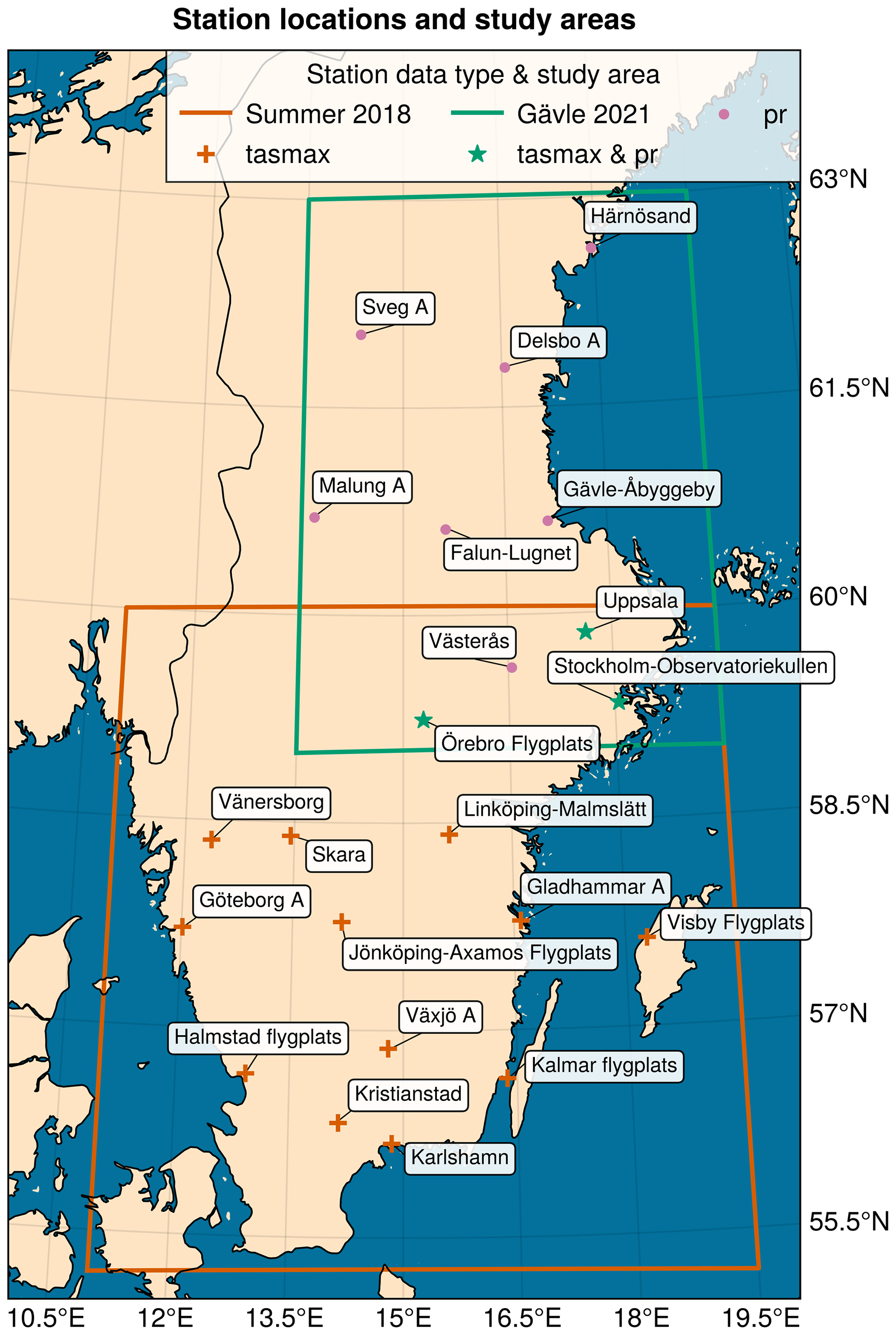
Figure 1Domain outlines and the locations of stations used in the study. Purple dots represent stations used only for precipitation data, the orange plus symbols represent those used for temperature data, and green stars show stations used for both precipitation and temperature. Coloured boxes show the outlines for the regions used in the selection of the gridded data.
We used the following gridded datasets: GridClim (Andersson et al., 2021), PTHBV (Gävle only; Johansson and Chen, 2005; Alexandersson, 2003; Johansson, 2000; Johansson and Chen, 2003), E-OBS (Cornes et al., 2018), and ERA5 (Hersbach et al., 2020). Additionally, we also used a bias-adjusted (Berg et al., 2022), 66-member version of the EURO-CORDEX ensemble (CORDEX stands for Coordinated Regional Climate Downscaling Experiment; Coppola et al., 2021; Jacob et al., 2014), as described in Kjellström et al. (2022). GridClim, E-OBS, ERA5, and the CORDEX ensemble all provided data until the end of 2018, while PTHBV covered up until the end of 2021. To assess how well the individual members of the CORDEX ensemble represented observations, we computed four metrics, all as total deviations: the annual averages, the monthly averages, the seasonal cycle, and the spatial patterns in the annual averages, between 1989 and 2018 for the respective domains using GridClim as the reference dataset. For definitions of the metrics, we refer to the report on the Bavarian climate projection ensemble (Bayerisches Landesamt für Umwelt, 2020). For all datasets, grid points outside the Swedish mainland were masked.
For each dataset, we used 30 years of daily data to define the period representing the recent past. In the context of analysing return times of extreme events, 30 years is a rather short period, and using a longer time series is generally desirable, and with the WWA method, it is advised to use as many data as possible. However, for this study, we chose a shorter period for two reasons. Firstly, we wanted to keep the period defining the climate of the recent past the same for both methods. Secondly, we wanted the period defining the current climate to be relatively stationary, limiting the climate signal from local changes in, for example, aerosol emissions.
The summer of 2018 in Sweden was characterised by several long-lasting high-pressure weather situations. This led to a record number of warm days, which was one of the unique features of that summer (Wilcke et al., 2020). Consequently, we define the summer 2018 event using the txge25 index (the number of days with a maximum temperature ≥25 °C), since that better reflects the longevity of the event rather than capturing the intensity on any single day or in any short period. To compute txge25, we used daily maximum temperatures between 1989 and 2018. The txge25 index is similar to the more common indicator SU (often referred to as summer days), defined as the number of days when Tmax>25 °C. For model data, where the number of reported decimals are plenty, this choice has little to no consequence. For observations, however, and specifically from manual historical records, there is a notable difference between counting days when tasmax>25 °C and where tasmax≥25 °C. The reason for this is that decimal points were not prioritised in early observational practices; e.g. a thermometer displaying 25.4 °C may have been recorded as 25 °C. In our case, the average median fraction attributable risk (FAR) for the summer 2018 event using the PI method decreased from ∼0.65 for the SU index to ∼0.48 for the txge25 index, an indication that using the former index results in an underestimation of warm days in the pre-industrial period.
August 2021 came with large amounts of precipitation in southern Sweden. The most intense event resulted in more than 100 mm in 24 h between 17 and 18 August for a large area close to the city of Gävle, which was highly impacted by the resulting flooding. For a relatively short-lived event like this, we chose to define the Gävle 2021 event using the Rx1day index (the maximum 1 d precipitation). Thus, for the Gävle event, we used the daily precipitation flux between 1991 and 2021. For both the events, we chose to include the events under investigation in the time series used in the following analysis.
We calculated the indicators using the software Climix (Zimmermann et al., 2023). For the summer 2018 event, only days within the period from May to August (MJJA) were used to calculate txge25, while Rx1day was calculated over the entire year. Furthermore, for the index describing the summer 2018 event, we calculated the domain average for each year. Since heavy-precipitation events are generally more localised compared to heat waves, we instead opted to calculate the annual domain maxima for the index describing the Gävle 2021 event.
2.2 Attribution using the WWA method
The rapid attribution framework from Philip et al. (2020) is a risk-based approach to attribution. It consists of steps outlining the preparations, analysis, and communication of an attribution study. In the following section, we will describe parts of the statistical method outlined in the framework.
The final result of a probabilistic attribution study is the probability ratio (PR),
or fraction of attributable risk (FAR),
where p1 and p0 are the probabilities of observing an event of a magnitude equal to or greater than the event threshold (exceedance probability) in the factual (current climate) and counterfactual (pre-industrial climate) worlds (see Fig. 2). PR and FAR are interchangeable, and which one to use depends on how the results will be presented. PR is interpreted as how many times more likely (or unlikely if <1) an event with the same magnitude has become. FAR instead describes the proportion of events of the same or greater magnitude that can be attributed to the changed forcing. For instance, if the PR of an event is 2, the interpretation would be that it has become twice as likely. On the other hand, the interpretation of the corresponding FAR =0.5 is that half of the occurrences of similar events can be attributed to the changed forcing.
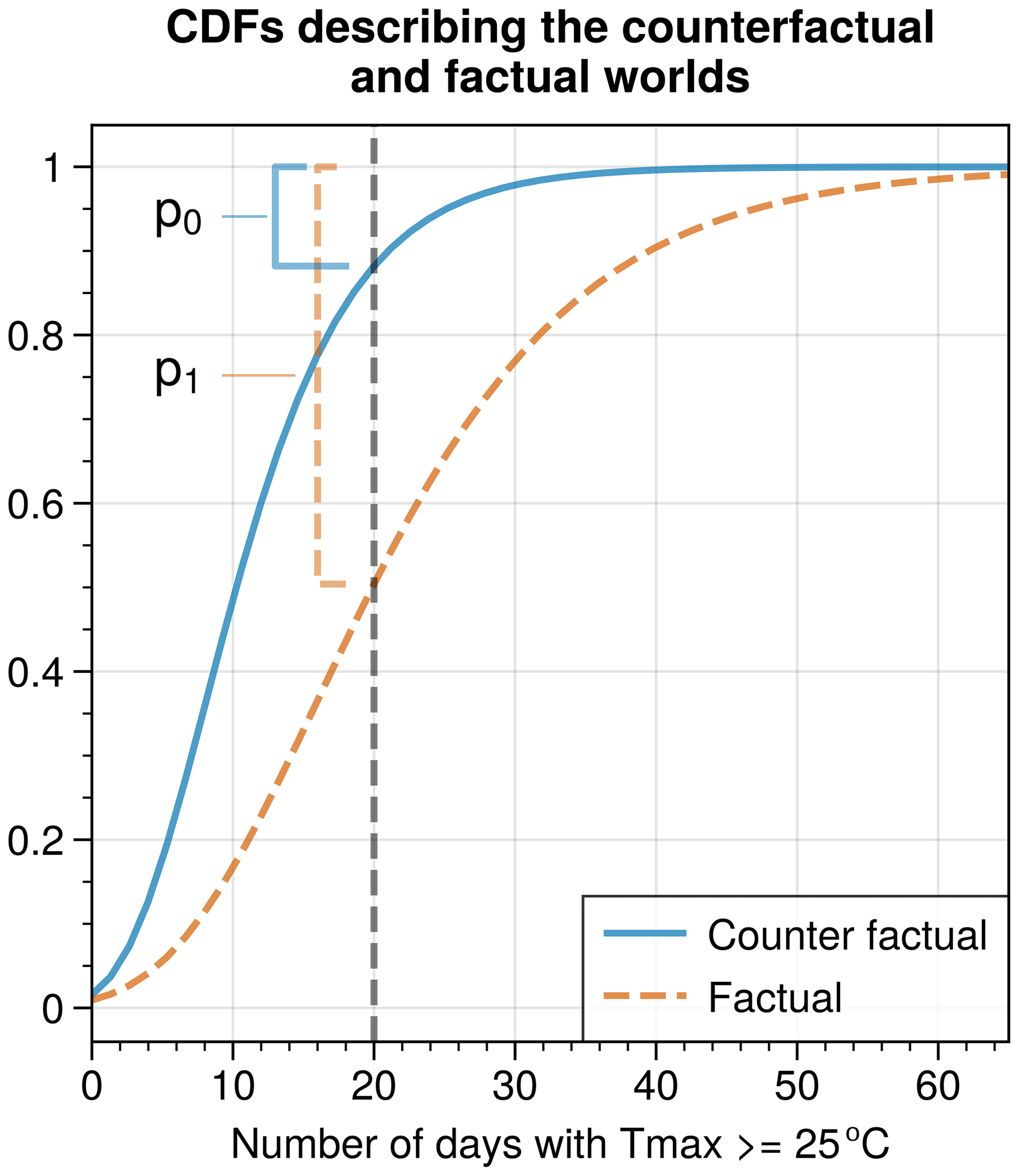
Figure 2Conceptual image describing the relationship between CDF and probability. Here, the two CDFs describe the distributions of the annual number of days with Tmax ≥25 °C in a factual and counterfactual world. An event threshold of 20 d is indicated by the vertical grey line. The corresponding event probabilities p1 and p0 are visualised as square brackets. In this case, p1 is larger than p0, which indicates that a summer with 20 d or more with a daily maximum temperature ≥25 °C is more likely in the factual world.
To calculate p1 and p0, ideally long observational datasets and climate model output records, which contain periods that represent both the current and the pre-industrial climate, should be used. The exceedance probability of a class of events, in either of the two periods, can then be sampled from the continuous density function (CDF) of a theoretical distribution fit to data representing the period (see Fig. 2). In most cases, data describing the current climate are readily available, from either observations, reanalysis products, or models, and retrieving p1 is relatively trivial.
Computing p0 requires data covering the pre-industrial period. Unfortunately, continuous observations with good spatial coverage from pre-industrial times are rare. Instead, one option is to use the output of climate models. For instance, general circulation models (GCMs) that are part of the Coupled Model Intercomparison Project (CMIP; Eyring et al., 2016) have a pre-industrial control run which could be used to represent the pre-industrial climate in attribution studies. A drawback of the GCMs is that their resolution is generally too low to properly represent many extreme weather events. The increased resolution of regional climate models (RCMs), for instance members of the CORDEX (Jones et al., 2011) ensemble, enables better representation of extreme weather events. However, the high-resolution runs completed in CORDEX traditionally do not include the pre-industrial control period, and thus they only cover a period from the middle of the 20th century onwards.
A third option used to represent the pre-industrial climate, which is used in this and many other attribution studies, is to shift or scale the distribution that represents the current climate. This relies on the assumption that the variable used to describe the event shifts or scales with a forcing that has a known climate change signal and historical record. An example of this is the global mean surface temperature (GMST), commonly used as a key indicator of climate change (e.g. Gulev et al., 2021).
The location μ of a distribution is shifted following
Here μ0 is the initial location, β is the coefficient of the linear regression between the variable and GMST, and ΔT is the change in GMST between the current and pre-industrial period. If the variable is instead assumed to scale with GMST, which is the case for precipitation, μ and the standard deviation σ are changed following
and
Either of these approaches will result in a distribution that represents the pre-industrial climate, where the CDF can be sampled to retrieve p0 (see Fig. 2).
We computed the linear regression between the 4-year rolling mean GMST (Hansen et al., 2010) and the 30-year annual time series of each index. For all datasets, we used the regression coefficients to detrend the index series of the current climate. For each index series, we then fit and evaluated a number of common extreme-value distributions and selected one for further analysis (see Sect. 2.4). We then used the regression coefficients (β) to shift and scale, respectively, the index distributions describing the summer of 2018 and Gävle 2021 events according to Eqs. (3), (4), and (5). This differs slightly from Philip et al. (2020), where they estimate β, μ, and σ, along with any other model parameters, directly from Eqs. (3), (4), and (5), using the longest time series available rather than a subset as used here. However, since the distributions used in this analysis were found to be invariant to linear transformations (not shown), this does not affect the outcome. For the CORDEX ensemble, the regression coefficient of each ensemble member was used as an additional quality control, where we removed any ensemble member where the regression coefficient exceeded the 95 % confidence interval of the regression in the reference dataset (GridClim). For each dataset, the distribution of the current climate and the pre-industrial (shifted/scaled) distribution formed a pair from which p1 and p0 could be retrieved and used to calculate FAR/PR (Eqs. 1 and 2). The threshold used for the summer 2018 event was based on the 2018 domain average txge25 in the GridClim product, whereas we used the 2021 domain maximum Rx1day in PTHBV for the Gävle 2021 event. For the gridded observations (GridClim, PTHBV, E-OBS, ERA5) we calculated confidence intervals with a bootstrap of randomly re-sampling the 30-year index series and performing the previous steps 1000 times. For the CORDEX data, instead of bootstrapping the confidence intervals, FAR from each ensemble member was used to form the distribution from which the confidence intervals could be retrieved.
2.3 Attribution using the PI method
As an alternative to the WWA method, we performed an attribution analysis employing several stations with long observational records of daily data. First, we merged a set of stations parameters, as is commonly done at SMHI, to extend and fill the gaps in the observational records for temperature and precipitation (e.g. Joelsson et al., 2022). This approach merges nearby stations which are assumed to be representative of the same geographic location but have different temporal coverage. The observational records were checked for missing values, and any stations missing ≥15 % of the days in the investigated period, during at least 1 year, were flagged in the subsequent analysis.
For each event, we selected all stations located inside the domain on the Swedish mainland and the island Gotland (Fig. 1). For both events, the pre-industrial period was defined as 1882 to 1911. This represents a period largely unaffected by anthropogenic climate change, yet it is relatively well covered in the observational records. The current climate period for the summer of 2018 was defined as 1989 to 2018 and for the Gävle 2021 event as 1992 to 2021. We calculated the same climate indices as for the gridded datasets (see Sect. 2.1) for each station. Following the index calculations, we further refined the station selection by requiring each station to provide a continuous 30-year period for both the pre-industrial and the current period. The selection procedure resulted in 15 stations for the 2018 event and 10 stations for the 2021 event. The locations and names of these stations are shown in Fig. 1. We checked the two separate periods of each station dataset for stationarity using the Kwiatkowski–Phillips–Schmidt–Shin (KPSS) and augmented Dickey–Fuller (ADF) tests (see Appendix A).
The two periods representing the pre-industrial climate and that of the recent past were then used to calculate PR and FAR following Eqs. (1) and (2), in the same way as done in the probabilistic event attribution (Sect. 2.2). Here, the threshold for the summer of 2018 was set to the 2018 station-averaged txge25, while the value of Rx1day for Gävle-Åbyggeby in 2021 was used as a threshold for the Gävle event. Furthermore, we also computed FAR for each station using the WWA method.
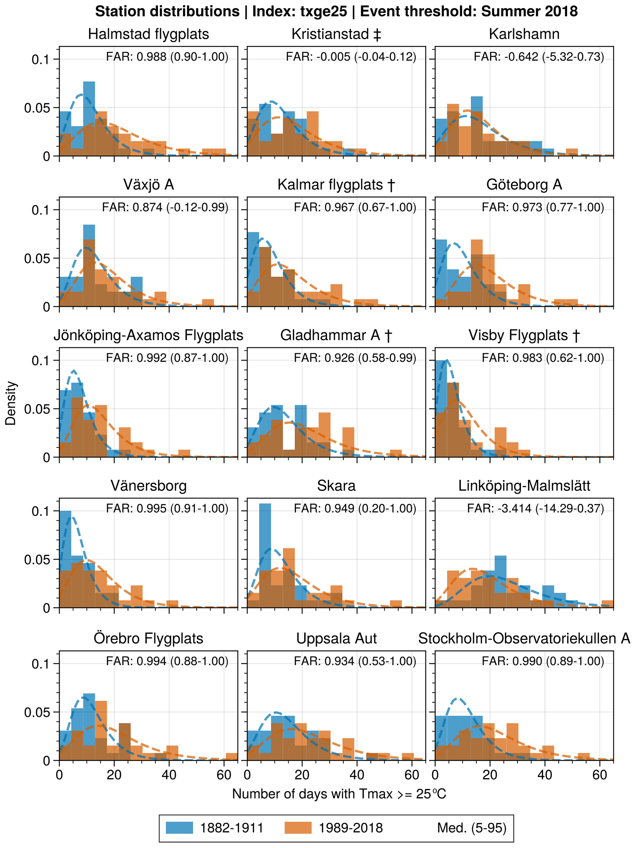
Figure 3Histograms of the txge25 index for the periods 1882–1911 and 1989–2018. Dashed lines show the probability density function (PDF) of the Gumbel distribution fit to each period. † indicates that at least 1 year misses 15 % of the days in the pre-industrial period. ‡ is the equivalent for the current period.
2.4 A note on distributions
In this study, we used the Python package SciPy (Virtanen et al., 2020) to fit, evaluate, and sample the distributions used to represent the data. There are multiple distributions suitable to represent extreme distributions, for instance generalised extreme value (GEV), Gaussian, generalised Pareto distribution (GPD), or Gumbel, and we refer to Philip et al. (2020) for further details on the selection of distributions. It is common practice to use a goodness-of-fit test, such as the Kolmogorov–Smirnov test (KS test), to evaluate the suitability of the different distributions to represent the data. However, we have found that relying solely on the KS test for selecting the appropriate distribution insufficient. Most notably, while the GEV distribution tends to show the highest performance in the KS test, it often results in division by zero errors in Eq. (1) for very high quantiles. The right-skewed Gumbel distribution does not lead to the same division by zero errors, while it still shows good performance in the KS test. A theoretical explanation for this is that the GEV distribution has a finite upper bound when the shape parameter is negative, which can result in events becoming theoretically impossible. The Gumbel distribution, on the other hand, has no upper bound since its shape parameter is fixed at zero, and events are never theoretically impossible. Because of this, we opted to use the right-skewed Gumbel distribution for all probability estimations in this analysis. It is worth noting that neither the Gumbel nor the GEV distribution is theoretically justified for count data, as is given by the txge25 index. However, the results of the KS test indicated that both the GEV and the Gumbel distributions were able to represent the txge25 data.
3.1 Summer of 2018
Almost all the stations employed in the analysis (Fig. 1) recorded ≥50 d with daily maximum temperatures ≥25 °C (summer days) during the summer of 2018 (Fig. A2), here defined as May to August (MJJA). There are only a few stations where this is not, by some margin, the highest number of summer days recorded between 1989–2018. Between 1882–1911, there are no years that equal the number of summer days in 2018 among any of the stations (Fig. A3).
Histograms, along with the distributions, generally show a positive difference between the distributions of the current and the pre-industrial climate for txge25 (Fig. 3). Consequently, the PI method generally yields positive values for FAR, with medians >0.8 for most of the stations (Fig. 3). It is only Kristianstad, Karlshamn, and Linköping-Malmslätt (LM) that exhibit FAR medians <0. Here, a FAR ≤0 implies that no occurrences of an event of similar or greater magnitude can be attributed to the changed forcing. Furthermore, there are no spatial patterns over southernmost Sweden that could explain the negative FAR of LM and Karlshamn (Fig. 4).
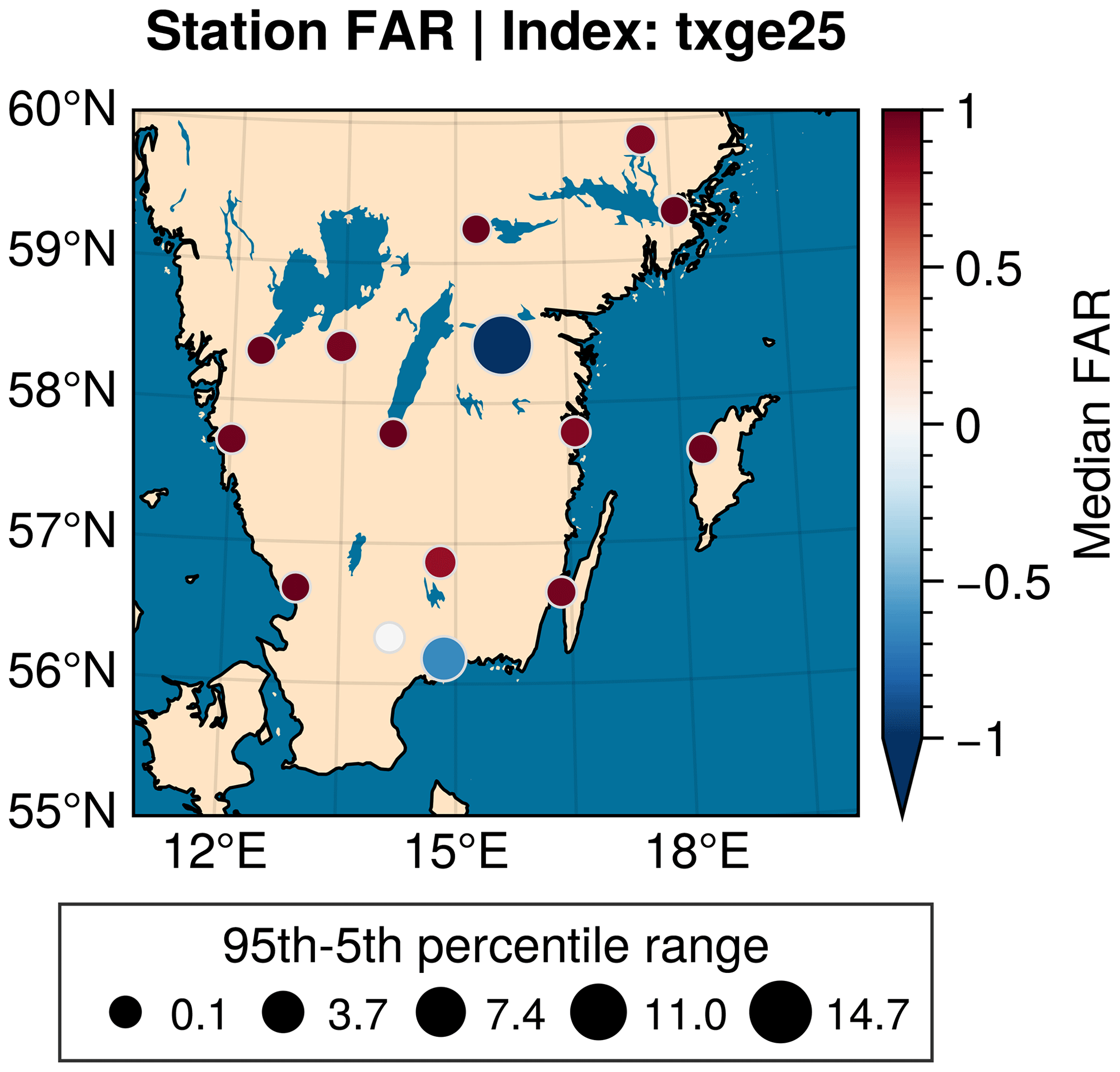
Figure 4FAR for the summer of 2018 at the stations used in the study. The marker colour represents the median FAR, while the marker size shows the uncertainty in FAR as the range between the 95th and 5th percentile.
Taking the average of the stations included in the PI method for the summer 2018 event gives a median FAR ∼0.50 with the 5th percentile (Q5) (Fig. 5). The FAR distributions (Fig. 5) further highlight the anomalous behaviour of LM, where neighbouring stations Skara, Gladhammar A, and Örebro Flygplats (see Figs. 1 and 4) display FAR distributions centred ≥0.75. For an adjusted average of the PI method (Fig. 5), where Karlshamn, Kristianstad, and LM are excluded, the median FAR ∼0.78 and Q5>0.1.
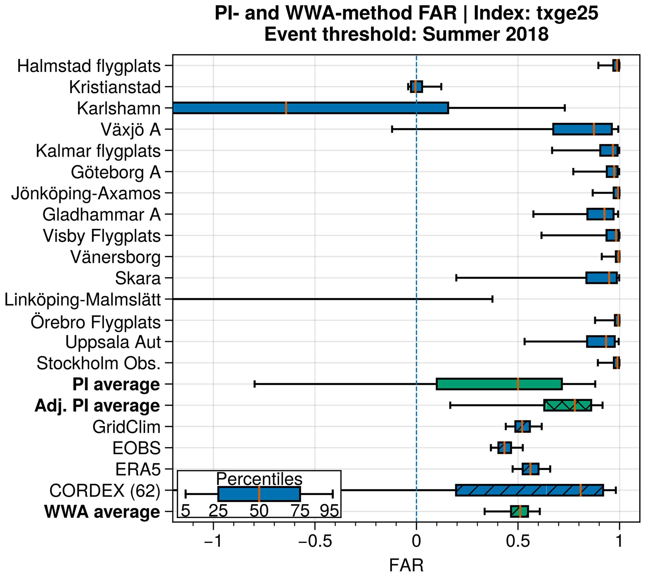
Figure 5FAR synthesis for the summer of 2018, as described by the txge25 index during MJJA. The bars represent the percentiles and median of the FAR distribution as described in the inset. Green bars denote the average for each method (PI and WWA). The WWA average here includes GridClim, E-OBS, ERA5, and the CORDEX ensemble. The green bar with crossed hatching (appearing as triangles) shows the adjusted average for the PI method, whereas the bars with parallel hatching (blue and green) display results from the WWA method. Note that the x axis is limited for increased readability.
The deviating results of these two stations are likely not the result of a local response to changes in climate. Instead, they are more likely a result of the station merging. In some cases, merging means that the station was moved to a new location. For LM, the station was moved a few kilometres west of central Linköping to the airfield at Malmslätt in 1943. Since temperatures are generally higher in urbanised areas due to the urban heat island effect (Rizwan et al., 2008), moving the station to a more rural area could introduce erroneous trends into the series (e.g. Tuomenvirta, 2001; Dienst et al., 2017). On the other hand, Karlshamn is an example of a station that provides a continuous observational record without merging or changes in location. Here, the implementation of thermometer screens during the 20th century, which generally results in reduced recorded temperatures, could be a part of the explanation.
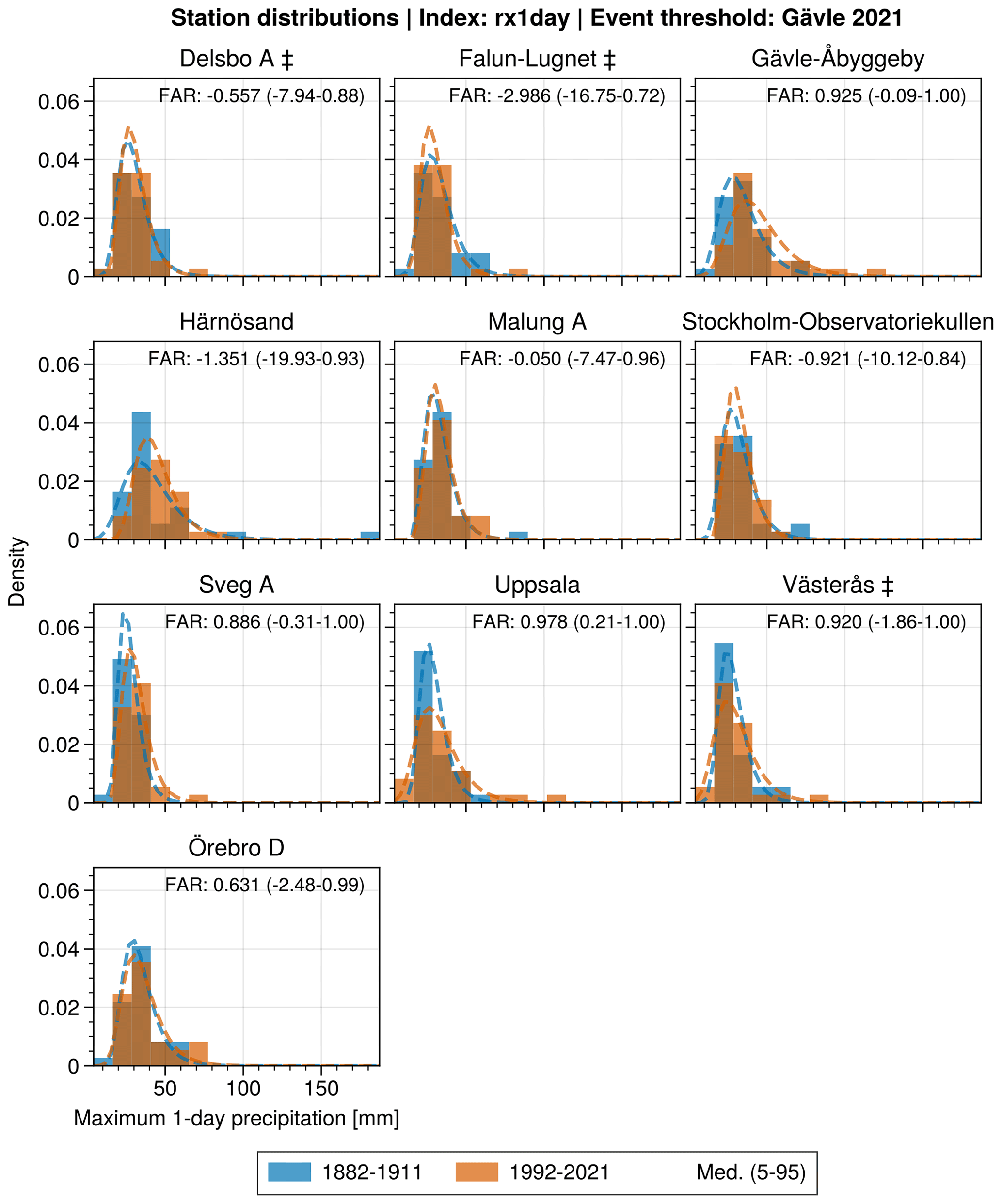
Figure 6Histograms of annual Rx1day for periods 1882–1911 and 1992–2021. Dashed lines show the PDF of the Gumbel distribution fit to each period. ‡ indicates that at least 1 year misses 15 % of the days in the current period.
These are examples of inhomogeneities in the observational record that make the investigation of trends and climate change difficult. Ideally, when working with signals of climate change in observational data, the data should first be homogenised; however, for daily data, this is currently not available in Sweden. Joelsson et al. (2022) present monthly averages of the 2 m temperature in Sweden from 1860, based on homogenised data from a high number of stations. The stations used in this study are a subset of the stations used in Joelsson et al. (2022). Since this study makes use of daily temperatures, we cannot directly utilise their results. However, their findings can help to further evaluate our results. In general, they found the required temperature corrections to be negative, with larger corrections during summers at the end of the 19th and beginning of the 20th century. This means that, generally, temperatures in the historical records were overestimated. For instance, their analysis indicates a homogeneity break in maximum temperature during 1890 for the station of Karlshamn, which coincides with the pronounced shift towards lower numbers in txge25 in Fig. A3. This implies that the estimated event probabilities during the pre-industrial period in this study are likely too high, which in turn results in an underestimation of FAR.
The analysis using the WWA method exhibits FAR similar to, albeit lower than, FAR estimated using the PI method (bottom five bars, Fig. 5). The FAR distributions for GridClim, E-OBS, and ERA5 all exhibit a median of 0.4–0.6 and a low spread, with 5th percentiles well above 0. The CORDEX ensemble FAR distribution, here with 62 members, shows a higher median (∼0.8), albeit with a greater spread (, Q95∼0.99) compared to the observation-based products (, Q95∼0.9). The WWA average (Fig. 5) shows the average FAR distribution of the datasets (GridClim, E-OBS, ERA5, CORDEX ensemble) used in the WWA method. Here, the median FAR is lower compared to the adjusted station average of the PI method, but uncertainty ranges overlap.
3.2 Gävle 2021
During the event on 17–18 August 2021, the station Gävle-Åbyggeby measured 121 mm of precipitation in 24 h. This was also the annual maximum 1 d precipitation (Rx1day) at that station in 2021. In 2021, none of the other assessed stations in the study area (Fig. 1) recorded a similar amount of precipitation in a single day. However, there are years in the recent past with annual daily maxima similar to the Gävle 2021 event, both in Gävle and at other stations (Fig. A4). In the pre-industrial period, there were only two recorded events, both in Härnösand, with similar magnitudes to the 2021 event (Fig. A5).
For an event like the heavy-precipitation event in Gävle in 2021, differences between the distributions of the pre-industrial and current climate are small at most of the 10 stations used to investigate the event (Fig. 6). There are a few stations (e.g. Gävle-Åbyggeby, Härnösand, Sveg A) that exhibit larger differences between the two periods, most notably in the tails of the distributions.
The FAR synthesis of the PI method (Fig. 7) shows the large variability among the stations. Here, Uppsala is the only station where the confidence interval does not include 0, Q5 ∼0.2. When looking at the median, however, Gävle-Åbyggeby, Sveg A, Uppsala, Västerås, and Örebro D all exhibit FAR >0. The remaining stations (Falun-Lugnet, Härnösand, Malung A, Stockholm-Observatoriekullen) show a median FAR ≤0. These differences are reflected by the large spread and negative median () of the average of the stations used in the PI method for the Gävle event (Fig. 7).
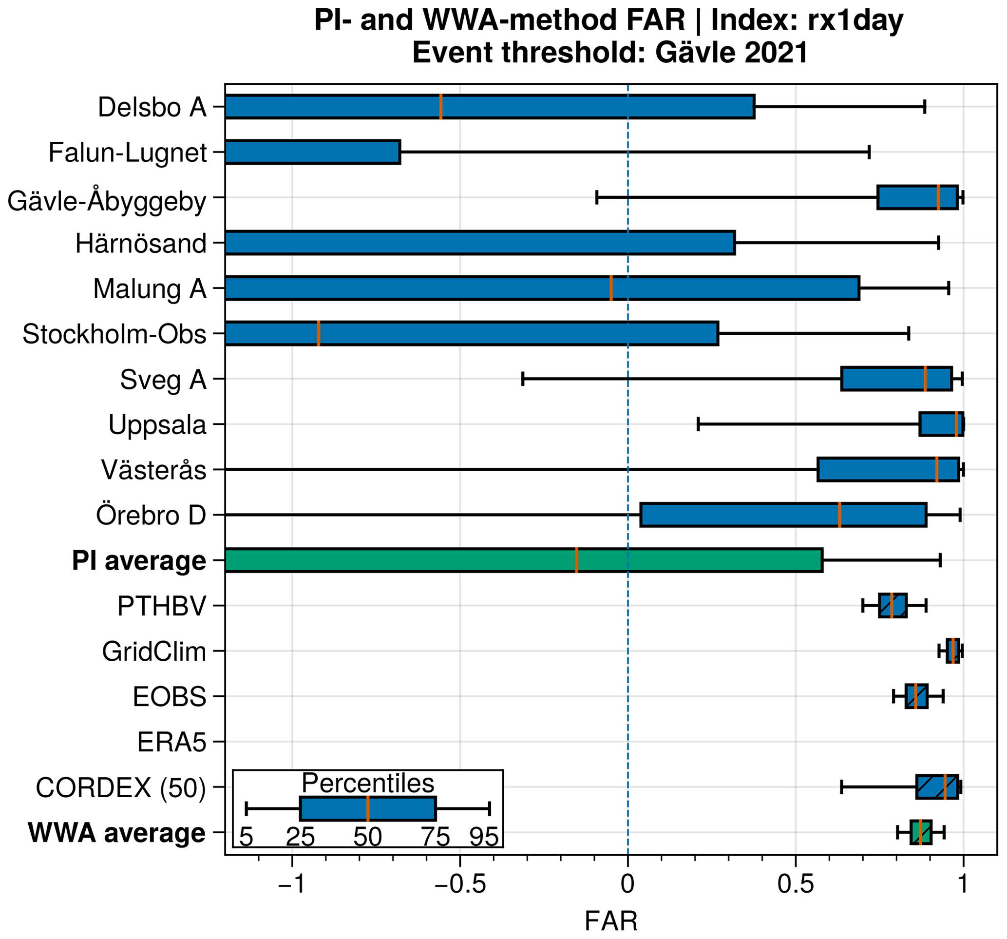
Figure 7FAR synthesis for the heavy-precipitation event in Gävle in 2021 described by the annual maximum 1 d precipitation (Rx1day). The bars represent the percentiles and median of the FAR distribution as described in the inset. Green bars denote the average for each method (PI and WWA). The WWA average here includes PTHBV, GridClim, E-OBS, and the CORDEX ensemble. The hatched bars (blue and green) display results from the WWA method. Note that the x axis is limited to −1 for readability. The ERA5 FAR distribution lies below this range and is not displayed.
FAR distributions from the WWA method for the Gävle 2021 event are shown with the hatched bars in Fig. 7. PTHBV, GridClim, E-OBS, and CORDEX exhibit similar medians (0.78–0.98), and Q5≥0.6. The results from ERA5 do not match the other datasets, with a median FAR and . We also note that ERA5 exhibits a negative regression to GMST, as opposed to the other datasets where the regression is generally positive. A contributor to this could be the overall underestimation of Rx1day in ERA5 found by Lavers et al. (2022). This requires further investigation, and we chose not to include ERA5 in the datasets used in the WWA average (PTHBV, GridClim, E-OBS, CORDEX ensemble).
For the Gävle event, there is some disagreement between the WWA method and the PI method. For stations such as Gävle-Åbyggeby, Sveg A, Uppsala, Västerås, and Örebro D, the median FAR derived by the PI method is of the same magnitude as that of the WWA method. However, the uncertainties are generally greater for the stations used in the PI method, with 5th percentiles <0 for multiple stations. Here, the difference in the magnitude of uncertainty between the two methods can likely be attributed to the fact that gridded data typically do not represent extreme precipitation events as well as local observations and thus have an overall lower variability. Furthermore, the relatively short 30-year period used to represent the current climate further limits how accurately the gridded datasets can represent the variability. This can lead to unstable estimates of p0 and p1 and unreliable estimates of FAR.
The question of homogeneity in the station data also applies to the precipitation measurements. During the later parts of the 20th century, many stations were converted from manual to automatic operation in Sweden. Here, the placement of automatic stations was generally in areas more exposed to wind compared to manual stations, and comparisons have shown that automatic measurements generally show less precipitation compared to those of manual stations (Alexandersson, 2003).
The two 30-year periods used to represent the pre-industrial (1882–1911) and the current (1992–2021) climate were found to be stationary at most of the stations (Figs. A5 and A4). Based on this, we decided not to detrend the station data. This also kept the following analysis (PI method) closer to the actual observations, not adding a dependence on regressions to, for example, GMST. Comparing the pre-industrial and current climate, most of the stations show distributions with very similar means (Fig. 6). In these cases, the results are more sensitive to the randomness of the bootstrap, resulting in the large uncertainties for some stations in Fig. 7.
3.3 Comparing the PI and WWA methods
With the long observational time series, we can further evaluate to what degree the PI method and WWA method agree. Here, in addition to using the PI method to estimate FAR, we applied the WWA method to the observations of the current climate (1989–2018 and 1991–2021, respectively) at each of the stations for the two events. The results are presented as FAR distributions for the two events in Figs. 8 and 9.
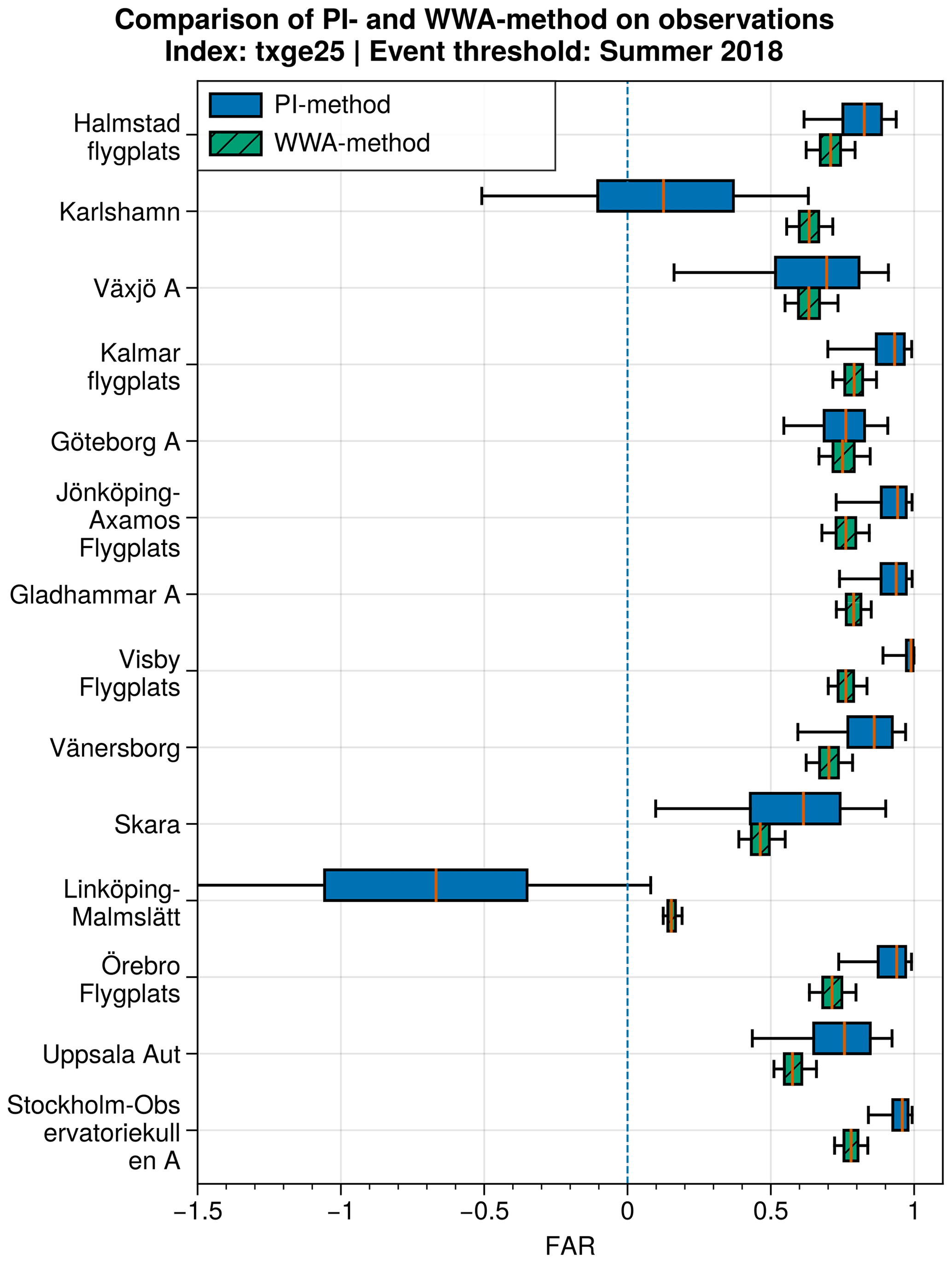
Figure 8Comparison of FAR distributions for the summer of 2018 from the PI method and WWA method applied to txge25 observations of the recent past. The first of the two bars (blue) in every pair shows the FAR distribution of the PI method, equivalent to what is shown in Fig. 5. The second bar (green, hatched) shows the FAR distribution from applying the WWA method to the time series of observations of the recent past for each station.
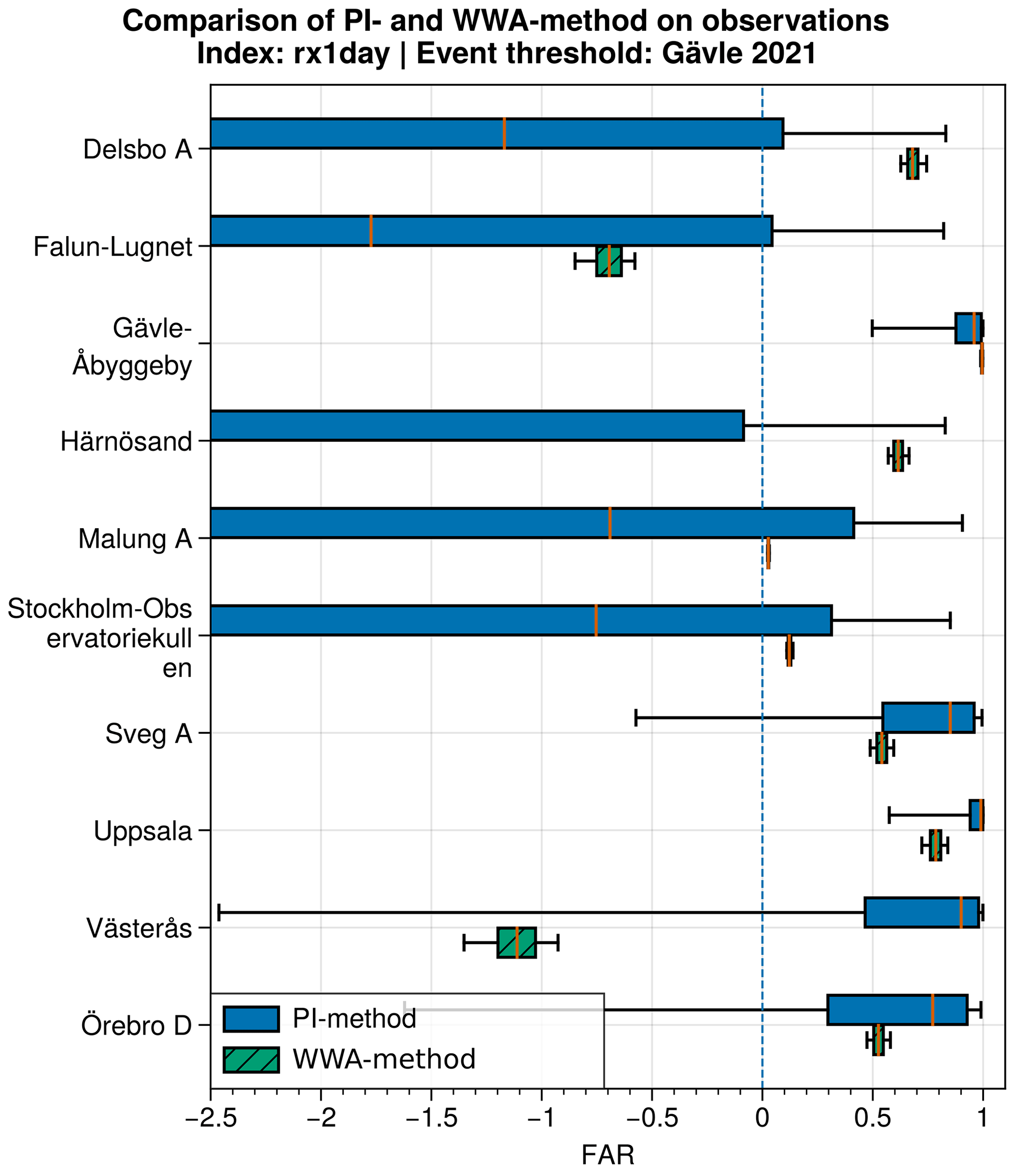
Figure 9Comparison of FAR distributions for the Gävle 2021 event from the PI method and WWA method applied to Rx1day observations of the recent past. The first of the two bars (blue) in every pair shows the FAR distribution of the PI method, equivalent to what is shown in Fig. 7. The second bar (green, hatched) shows the FAR distribution from applying the WWA method to the time series of observations of the recent past for each station.
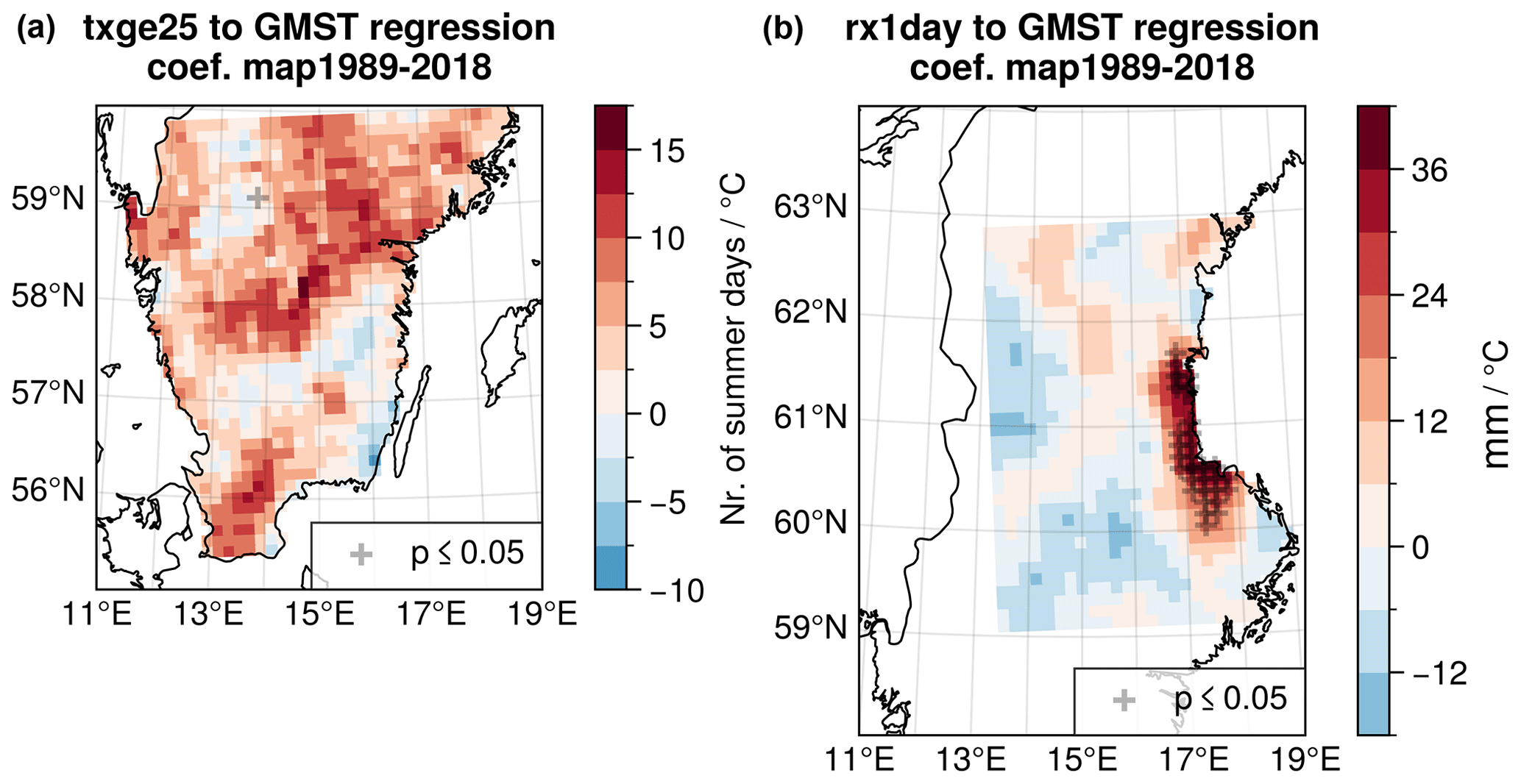
Figure 10Gridded maps showing the regression coefficients between GMST and GridClim for (a) the txge25 index over the summer 2018 domain during 1989–2018 and (b) the Rx1day index over the Gävle event domain during 1989–2018. Crosses indicate significance at p≤0.05. For the summer 2018 domain, the spatial variability is relatively low, with few grid points showing a significant regression. While the Gävle domain shows a cluster of points with a significant regression along the coast between 60 and 62° N, the overall spatial variability is greater compared to the summer of 2018.
The results clearly show that the two methods generally yield similar results for the summer of 2018 (Fig. 8), albeit with somewhat lower FAR numbers for the WWA method compared to the PI method. This is likely a result of the weak regression coefficient between the variable (txge25) and GMST (Fig. A1). Figure 3 gives some indication that the scale of the distributions varies between the pre-industrial climate and that of the climate of the recent past for a few stations (e.g. Halmstad Flygplats, Vänersborg). This conflicts with the notion that temperature distributions shift following the regression to GMST, which is utilised in the WWA method. An implication of this is a shifted distribution that is too wide, giving higher estimates of p0 and consequently a lower FAR, which could explain the differences we observe between the two methods here. There are two stations, Karlshamn and Linköping-Malmslätt, where the WWA method results in a higher estimation of FAR compared to the PI method. Interestingly, for both these stations, the WWA method yields FAR distributions that are more aligned with the FAR (WWA and PI) of the other stations used in the analysis. Overall, this suggests that the WWA method, even when applied to only 30 years of data, can capture changes in probabilities for a larger-scale temperature-related event such as the one in the summer of 2018. Furthermore, this indicates that the relationship between GMST and local temperature extremes in this area has remained relatively constant throughout the 20th century.
For the Gävle event, differences between the FAR distributions for the WWA method and the PI method are more varied (Fig. 9). For several stations, the FAR distributions of the WWA method and PI method generally agree (e.g. Gävle-Åbyggeby, Sveg A, Uppsala, Örebro D). At the other stations, the median FAR from the two methods does not agree, but the uncertainty ranges of the FAR distributions still overlap, mostly due to the large uncertainty in FAR distributions of the PI method. Furthermore, the much smaller uncertainty in FAR distributions of the WWA method is an indication that the short time periods can lead to distributions that do not encompass the whole variability, as discussed above.
Figure 10 shows maps of the regression coefficients between GMST and the index series at the grid points in the two domains representing the events. For the domain representing the Gävle event, the regression between Rx1day (GridClim) and GMST (1989–2018) is relatively strong along and in proximity to the coast between 60 and 62° N (Fig. 10). Outside this sub-area, the regression is generally weaker and not statistically significant, with no distinguishable spatial patterns. In comparison, the regression between txge25 and GMST in the domain representing the summer 2018 event exhibits relatively small spatial variations over the domain (Fig. 10), but with fewer grid points showing a significant regression. This indicates that the extreme precipitation event is more sensitive to the choice of domain compared to the extreme temperature event.
We have applied two sets of attribution analysis to two notable extreme weather events in Sweden: the warm summer of 2018 and the heavy-precipitation event in Gävle in 2021. For the WWA method we made use of a number of gridded datasets covering the last few decades and assumed that the variable describing the event either shifted or scaled with GMST. This allowed us to calculate the exceedance probabilities, and their change, for the events from distributions that represent the climate in a pre-industrial period and during the recent past. For the PI method, we instead relied solely on observations to represent the climate during both the pre-industrial and the current periods to retrieve corresponding probabilities. We found the extensive observational record available in Sweden a valuable source of data that, if homogenised, could help to further clarify some uncertainties arising from using non-homogenised data.
For the summer of 2018, results from the PI method, excluding stations affected by inhomogeneities, exhibit a stronger attribution compared to the results of the WWA method. When applied to the station data used in the PI method, the WWA method also results in slightly lower values for FAR. The systematic difference between the two approaches using temperature data from the long-term stations indicates that this may be related to the regression between the temperature index (txge25) and GMST or the fixed-scale parameter of the shifted distributions. However, these differences are rather small, and overall, our results suggest that the WWA method can capture changes in probabilities for large-scale temperature-related events even when applied to only 30 years of data, which is shorter than what is recommended.
We also note that since high temperatures tend to be overestimated in historical observations, using homogenised observations is likely to result in a higher FAR for heat-wave-related extremes using the PI method. Furthermore, based on these results, we can conclude that one out of every two heat waves similar to the summer of 2018 can be attributed to changes in the climate. Alternatively, such heat waves have become twice as likely due to changes in the climate. When only using station data, the previous statement increases to more than two out of three and would likely be even higher using homogenised data.
Regarding the precipitation event in Gävle in 2021, results from the PI method are highly variable, making the attribution of the event uncertain. Here, 5 out of 10 stations exhibit a median FAR >0.5, but only 1 displays FAR that is significantly above 0. On the other hand, except for the ERA5 dataset, there is a fairly good agreement among the gridded datasets analysed using the WWA method, and the method shows a stronger attribution compared to the PI method. Applying the WWA method to the station data used in the PI method does not reveal any positive or negative tendency when comparing the results of the two methods. These large variations within and between the two methods make it difficult to draw any conclusions regarding the attribution of the extreme precipitation event in Gävle in 2021.
Comparing the two events, the regression maps indicate that a precipitation event like the one in Gävle appears to be more sensitive to the choice of domain than a more widespread and uniform heat wave like the one in the summer of 2018. This also agrees with previous findings indicating that extreme precipitation events are more sensitive to the event definition.
Regarding the more generally applicable WWA method for attribution, future studies should try to utilise as many data as possible and continue to explore how the regional variations in relationships, such as that between the local Clausius–Clapeyron scaling and GMST, affect the outcome of studies on extreme event attribution.
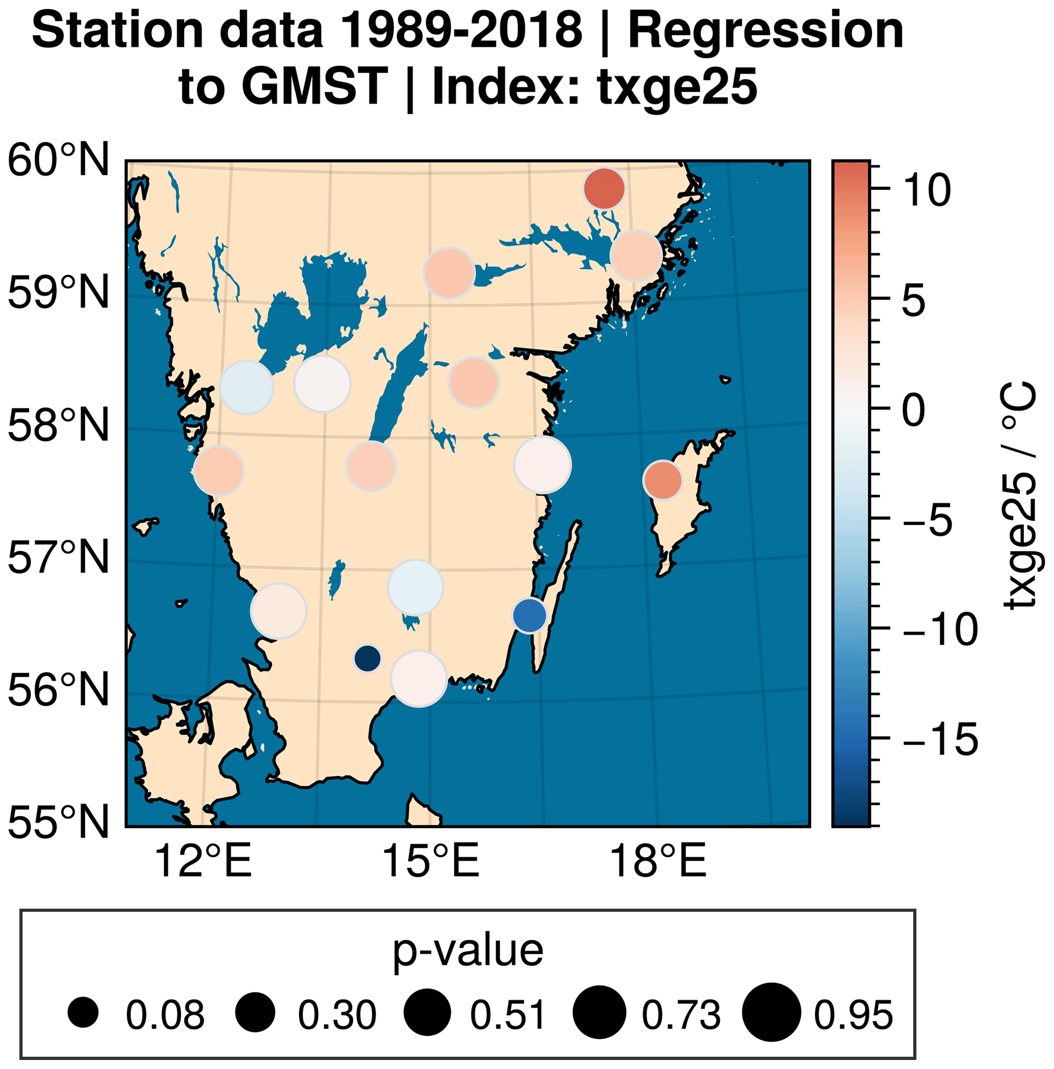
Figure A1Regression between the index series and GMST at the respective stations. The strength and sign of the regression coefficient are indicated by the colour, while the size of the markers indicates the p value.
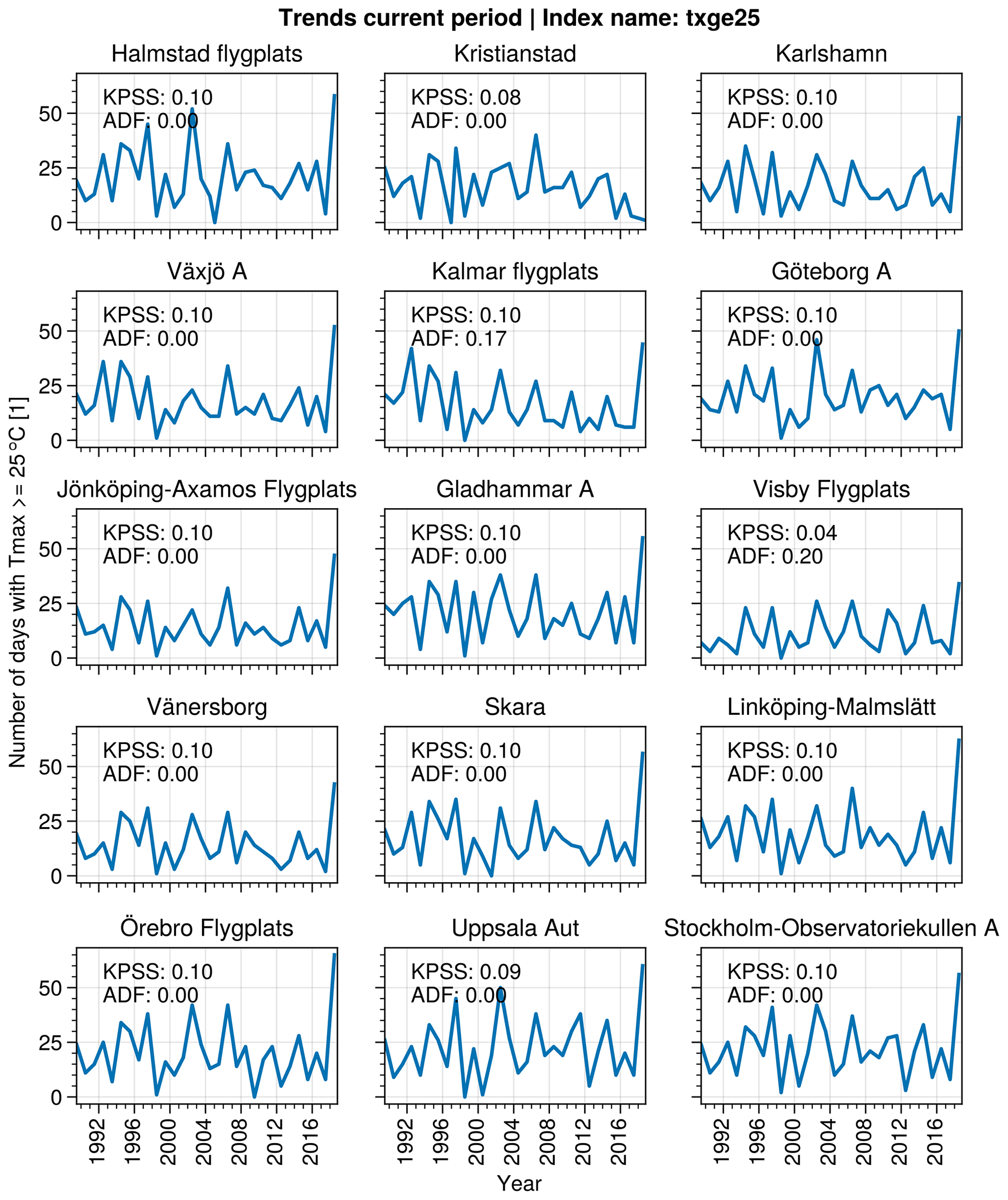
Figure A2Trend analysis of the current period (1989–2018) for the txge25 index. KPSS ≤0.05 indicates that a series is non-stationary. ADF ≤0.05 indicates that a series is trend stationary.
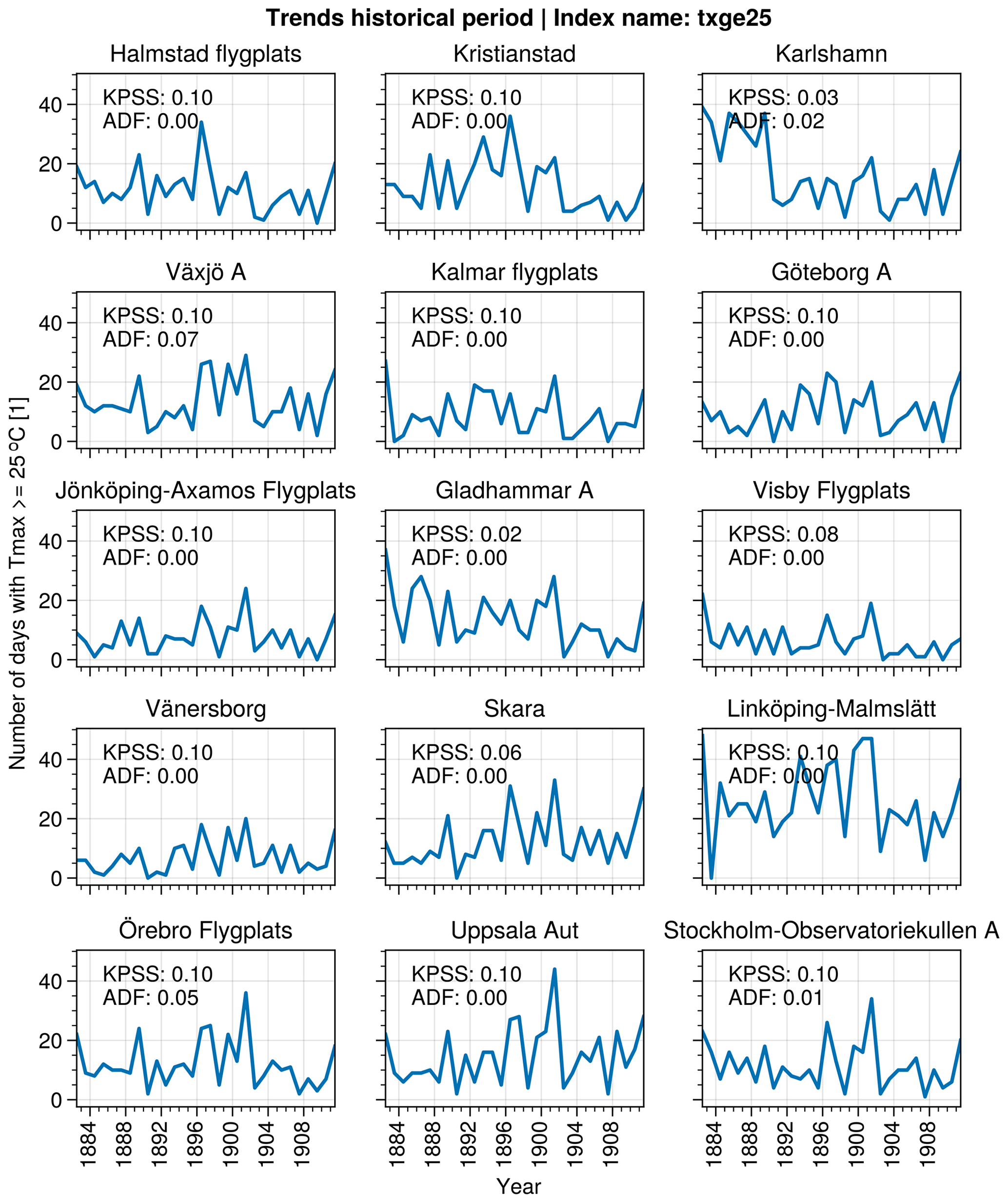
Figure A3Trend analysis of the historical period (1882–1911) for the txge25 index. KPSS ≤0.05 indicates that a series is non-stationary. ADF ≤0.05 indicates that a series is trend stationary.
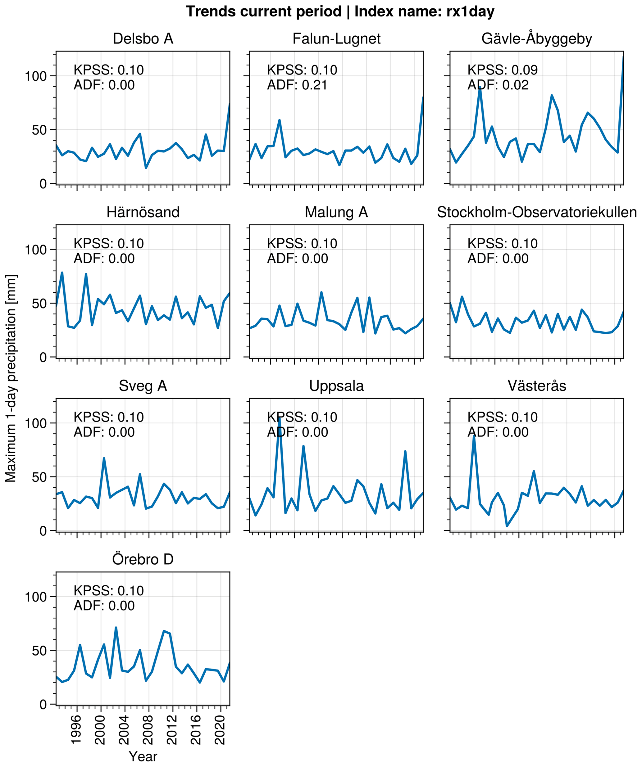
Figure A4Trend analysis of the current period (1991–2021) for the Rx1day index. KPSS ≤0.05 indicates that a series is non-stationary. ADF ≤0.05 indicates that a series is trend stationary.
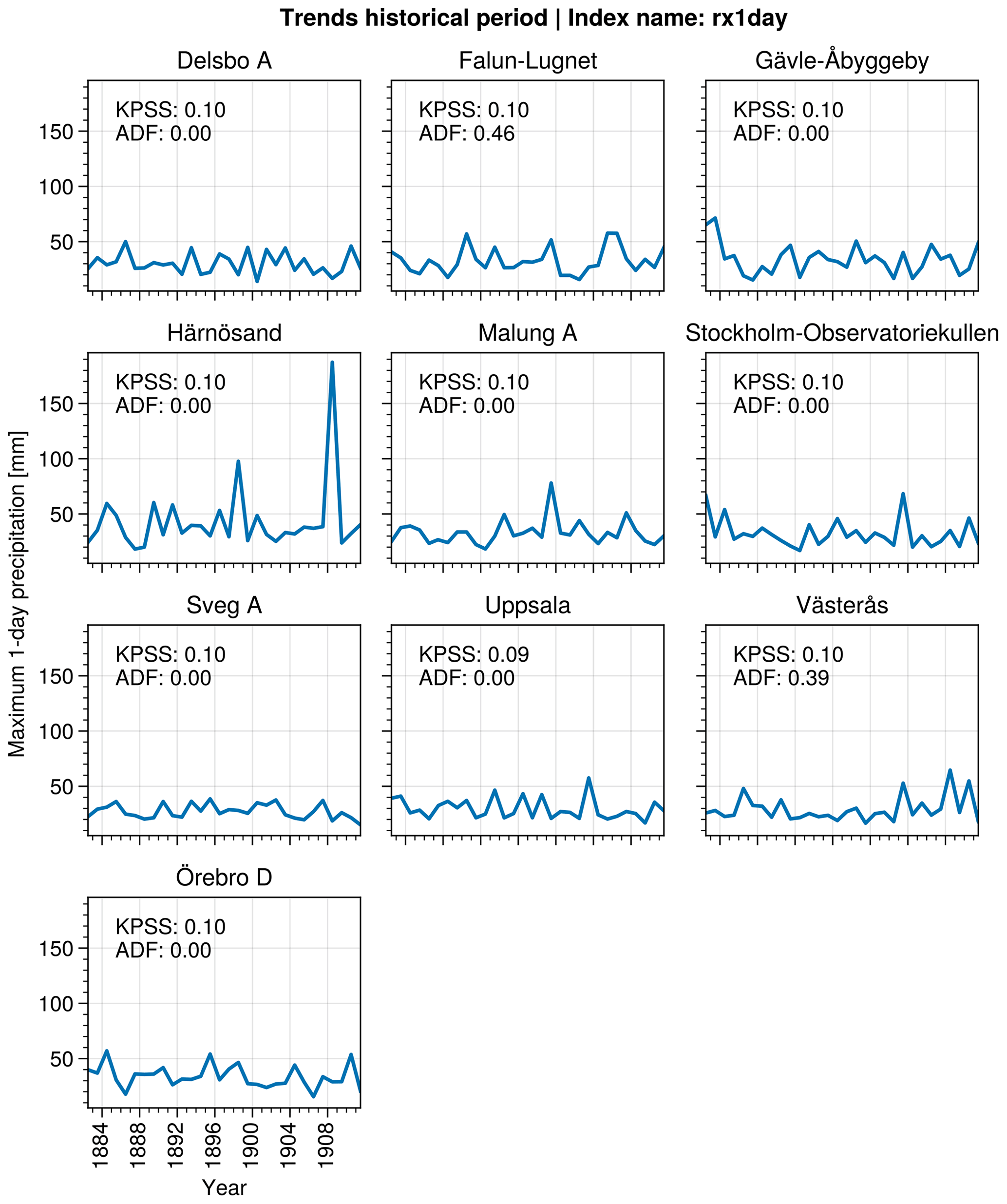
Figure A5Trend analysis of the historical period (1882–1911) for the Rx1day index. KPSS ≤0.05 indicates that a series is non-stationary. ADF ≤0.05 indicates that a series is trend stationary.
Code used in this analysis is available at https://doi.org/10.5281/zenodo.13358507 (Holmgren, 2024).
The station data and the GridClim and PTHBV datasets are freely available from the Swedish Meteorological and Hydrological Institute (https://www.smhi.se, Swedish Meteorological and Hydrological Institute, 2024).
CORDEX data are freely available from the Earth System Grid Federation (ESGF, https://esgf.llnl.gov/nodes.html, Earth System Grid Federation, 2024).
The ERA5 data used are freely available through the C3S Climate Data Store (https://cds.climate.copernicus.eu, Copernicus Climate Change Service, 2024).
The E-OBS data used are freely available through ECA&D (https://www.ecad.eu/, European Climate Assessment & Dataset project, 2024).
EH developed and carried out the analysis, prepared figures, and wrote the article. EK initiated the study, provided comments during the development of the analysis, and assisted in the revision of the article.
The contact author has declared that neither of the authors has any competing interests.
Publisher’s note: Copernicus Publications remains neutral with regard to jurisdictional claims made in the text, published maps, institutional affiliations, or any other geographical representation in this paper. While Copernicus Publications makes every effort to include appropriate place names, the final responsibility lies with the authors.
We would like to thank the two reviewers for their very valuable comments. Finally, we want to thank Johan Södling for his greatly appreciated guidance.
This research was funded by the Swedish Meteorological and Hydrological Institute, specifically the 1:10 government grant “Klimatanpassning”.
The publication of this article was funded by the Swedish Research Council, Forte, Formas, and Vinnova.
This paper was edited by Vassiliki Kotroni and reviewed by Vikki Thompson and one anonymous referee.
Alexandersson, H.: Korrektion Av Nederbörd Enligt Enkel Klimatologisk Metodikl, Tech. Rep., 111, SMHI, URN: urn:nbn:se:smhi:diva-2323, 2003. a, b
Andersson, S., Bärring, L., Landelius, T., Samuelsson, P., and Schimanke, S.: SMHI Gridded Climatology, SMHI, URN: urn:nbn:se:smhi:diva-6192, 2021. a
Bayerisches Landesamt für Umwelt: Das Bayerische Klimaprojektionsensemble Audit Und Ensemblebildung, Tech. rep., Bayerisches Landesamt für Umwelt, 2020. a
Berg, P., Bosshard, T., Yang, W., and Zimmermann, K.: MIdASv0.2.1 – MultI-scale bias AdjuStment, Geosci. Model Dev., 15, 6165–6180, https://doi.org/10.5194/gmd-15-6165-2022, 2022. a
Coppola, E., Nogherotto, R., Ciarlo', J. M., Giorgi, F., van Meijgaard, E., Kadygrov, N., Iles, C., Corre, L., Sandstad, M., Somot, S., Nabat, P., Vautard, R., Levavasseur, G., Schwingshackl, C., Sillmann, J., Kjellström, E., Nikulin, G., Aalbers, E., Lenderink, G., Christensen, O. B., Boberg, F., Sørland, S. L., Demory, M.-E., Bülow, K., Teichmann, C., Warrach-Sagi, K., and Wulfmeyer, V.: Assessment of the European Climate Projections as Simulated by the Large EURO-CORDEX Regional and Global Climate Model Ensemble, J. Geophys. Res.-Atmos., 126, e2019JD032356, https://doi.org/10.1029/2019JD032356, 2021. a
Copernicus Climate Change Service: ERA5 data, CDS [data set], https://cds.climate.copernicus.eu, last access: August 2024. a
Cornes, R. C., van der Schrier, G., van den Besselaar, E. J. M., and Jones, P. D.: An Ensemble Version of the E-OBS Temperature and Precipitation Data Sets, J. Geophys. Res.-Atmos., 123, 9391–9409, https://doi.org/10.1029/2017JD028200, 2018. a
Dienst, M., Lindén, J., Engström, E., and Esper, J.: Removing the Relocation Bias from the 155-Year Haparanda Temperature Record in Northern Europe, Int. J. Climatol., 37, 4015–4026, https://doi.org/10.1002/joc.4981, 2017. a
Doblas-Reyes, F., Sörensson, A., Almazroui, M., Dosio, A., Gutowski, W., Haarsma, R., Hamdi, R., Hewitson, B., Kwon, W.-T., Lamptey, B., Maraun, D., Stephenson, T., Takayabu, I., Terray, L., Turner, A., and Zuo, Z.: Linking Global to Regional Climate Change, in: Climate Change 2021: The Physical Science Basis. Contribution of Working Group I to the Sixth Assessment Report of the Intergovernmental Panel on Climate Change, edited by: Masson-Delmotte, V., Zhai, P., Pirani, A., Connors, S., Péan, C., Berger, S., Caud, N., Chen, Y., Goldfarb, L., Gomis, M., Huang, M., Leitzell, K., Lonnoy, E., Matthews, J., Maycock, T., Waterfield, T., Yelekçi, O., Yu, R., and Zhou, B., 1363–1512, Cambridge University Press, Cambridge, United Kingdom and New York, NY, USA, https://doi.org/10.1017/9781009157896.012, 2021. a
Dole, R., Hoerling, M., Perlwitz, J., Eischeid, J., Pegion, P., Zhang, T., Quan, X.-W., Xu, T., and Murray, D.: Was There a Basis for Anticipating the 2010 Russian Heat Wave?, Geophys. Res. Lett., 38, L06702, https://doi.org/10.1029/2010GL046582, 2011. a
Earth System Grid Federation: CORDEX data, ESGF [data set], https://esgf.llnl.gov/nodes.html, last access: August 2024. a
European Climate Assessment & Dataset project: E-OBS data, ECAD [data set], https://www.ecad.eu/, last access: August 2024. a
Eyring, V., Bony, S., Meehl, G. A., Senior, C. A., Stevens, B., Stouffer, R. J., and Taylor, K. E.: Overview of the Coupled Model Intercomparison Project Phase 6 (CMIP6) experimental design and organization, Geosci. Model Dev., 9, 1937–1958, https://doi.org/10.5194/gmd-9-1937-2016, 2016. a
Eyring, V., Gillett, N., Achuta Rao, K., Barimalala, R., Barreiro Parrillo, M., Bellouin, N., Cassou, C., Durack, P., Kosaka, Y., McGregor, S., Min, S., Morgenstern, O., and Sun, Y.: Human Influence on the Climate System, in: Climate Change 2021: The Physical Science Basis. Contribution of Working Group I to the Sixth Assessment Report of the Intergovernmental Panel on Climate Change, edited by: Masson-Delmotte, V., Zhai, P., Pirani, A., Connors, S., Péan, C., Berger, S., Caud, N., Chen, Y., Goldfarb, L., Gomis, M., Huang, M., Leitzell, K., Lonnoy, E., Matthews, J., Maycock, T., Waterfield, T., Yelekçi, O., Yu, R., and Zhou, B., 423–552, Cambridge University Press, Cambridge, United Kingdom and New York, NY, USA, https://doi.org/10.1017/9781009157896.005, 2021. a
Gulev, S., Thorne, P., Ahn, J., Dentener, F., Domingues, C., Gerland, S., Gong, D., Kaufman, D., Nnamchi, H., Quaas, J., Rivera, J., Sathyendranath, S., Smith, S., Trewin, B., von Schuckmann, K., and Vose, R.: Changing State of the Climate System, in: Climate Change 2021: The Physical Science Basis. Contribution of Working Group I to the Sixth Assessment Report of the Intergovernmental Panel on Climate Change, edited by: Masson-Delmotte, V., Zhai, P., Pirani, A., Connors, S., Péan, C., Berger, S., Caud, N., Chen, Y., Goldfarb, L., Gomis, M., Huang, M., Leitzell, K., Lonnoy, E., Matthews, J., Maycock, T., Waterfield, T., Yelekçi, O., Yu, R., and Zhou, B., 287–422, Cambridge University Press, Cambridge, United Kingdom and New York, NY, USA, https://doi.org/10.1017/9781009157896.004, 2021. a
Hansen, J., Ruedy, R., Sato, M., and Lo, K.: Global Surface Temperature Change, Rev. Geophys., 48, RG4004, https://doi.org/10.1029/2010RG000345, 2010. a
Herring, S. C., Christidis, N., Hoell, A., and Stott, P. A.: Explaining Extreme Events of 2020 from a Climate Perspective, B. Am. Meterol. Soc., 103, S1–S129, https://doi.org/10.1175/BAMS-ExplainingExtremeEvents2020.1, 2022. a
Hersbach, H., Bell, B., Berrisford, P., Hirahara, S., Horányi, A., Muñoz-Sabater, J., Nicolas, J., Peubey, C., Radu, R., Schepers, D., Simmons, A., Soci, C., Abdalla, S., Abellan, X., Balsamo, G., Bechtold, P., Biavati, G., Bidlot, J., Bonavita, M., De Chiara, G., Dahlgren, P., Dee, D., Diamantakis, M., Dragani, R., Flemming, J., Forbes, R., Fuentes, M., Geer, A., Haimberger, L., Healy, S., Hogan, R. J., Hólm, E., Janisková, M., Keeley, S., Laloyaux, P., Lopez, P., Lupu, C., Radnoti, G., de Rosnay, P., Rozum, I., Vamborg, F., Villaume, S., and Thépaut, J.-N.: The ERA5 Global Reanalysis, Q. J. Roy. Meteor. Soc., 146, 1999–2049, https://doi.org/10.1002/qj.3803, 2020. a
Hoerling, M., Kumar, A., Dole, R., Nielsen-Gammon, J. W., Eischeid, J., Perlwitz, J., Quan, X.-W., Zhang, T., Pegion, P., and Chen, M.: Anatomy of an Extreme Event, J. Climate, 26, 2811–2832, https://doi.org/10.1175/JCLI-D-12-00270.1, 2013. a
Holland, G. and Bruyère, C. L.: Recent Intense Hurricane Response to Global Climate Change, Clim. Dynam., 42, 617–627, https://doi.org/10.1007/s00382-013-1713-0, 2014. a
Holmgren, E.: Holmgren825/holmgren_kjellstrom_exploring_attribution: v1.0 (stable), Zenodo [code], https://doi.org/10.5281/zenodo.13358507, 2024. a
Jacob, D., Petersen, J., Eggert, B., Alias, A., Christensen, O. B., Bouwer, L. M., Braun, A., Colette, A., Déqué, M., Georgievski, G., Georgopoulou, E., Gobiet, A., Menut, L., Nikulin, G., Haensler, A., Hempelmann, N., Jones, C., Keuler, K., Kovats, S., Kröner, N., Kotlarski, S., Kriegsmann, A., Martin, E., van Meijgaard, E., Moseley, C., Pfeifer, S., Preuschmann, S., Radermacher, C., Radtke, K., Rechid, D., Rounsevell, M., Samuelsson, P., Somot, S., Soussana, J.-F., Teichmann, C., Valentini, R., Vautard, R., Weber, B., and Yiou, P.: EURO-CORDEX: New High-Resolution Climate Change Projections for European Impact Research, Reg. Environ. Change, 14, 563–578, https://doi.org/10.1007/s10113-013-0499-2, 2014. a
Joelsson, L. M. T., Engström, E., and Kjellström, E.: Homogenization of Swedish Mean Monthly Temperature Series 1860–2021, Int. J. Climatol., 43, 1079–1093, https://doi.org/10.1002/joc.7881, 2022. a, b, c
Johansson, B.: Areal Precipitation and Temperature in the Swedish Mountains: An Evaluation from a Hydrological Perspective, Hydrol. Res., 31, 207–228, https://doi.org/10.2166/nh.2000.0013, 2000. a
Johansson, B. and Chen, D.: The Influence of Wind and Topography on Precipitation Distribution in Sweden: Statistical Analysis and Modelling, Int. J. Climatol., 23, 1523–1535, 2003. a
Johansson, B. and Chen, D.: Estimation of Areal Precipitation for Runoff Modelling Using Wind Data: A Case Study in Sweden, Clim. Res., 29, 53–61, 2005. a
Jones, C., Giorgi, F., and Asrar, G.: The Coordinated Regional Downscaling Experiment: CORDEX, An International Downscaling Link to CMIP5, CLIVAR Exchanges, 16, 34–40, 2011. a
Kjellström, E., Andersson, L., Arneborg, L., Berg, P., Capell, R., Fredriksson, S., Hieronymus, M., Jönsson, A., Lindström, L., and Strandberg, G.: Klimatinformation som stöd för samhällets klimatanpassningsarbete, Tech. Rep. 64, URN: urn:nbn:se:smhi:diva-6228, SMHI, 2022. a
Lavers, D. A., Simmons, A., Vamborg, F., and Rodwell, M. J.: An Evaluation of ERA5 Precipitation for Climate Monitoring, Q. J. Roy. Meteor. Soc., 148, 3152–3165, https://doi.org/10.1002/qj.4351, 2022. a
Leach, N., Li, S., Sparrow, S., Van Oldenborgh, G. J., Lott, F. C., Weisheimer, A., and Allen, M. R.: Anthropogenic Influence on the 2018 Summer Warm Spell in Europe: The Impact of Different Spatio-Temporal Scales, B. Am. Meterol. Soc., 101, S41–S46, https://doi.org/10.1175/BAMS-D-19-0201.1, 2020. a
Olsson, L., Thorén, H., Harnesk, D., and Persson, J.: Ethics of Probabilistic Extreme Event Attribution in Climate Change Science: A Critique, Earth's Future, 10, e2021EF002258, https://doi.org/10.1029/2021EF002258, 2022. a
Otto, F. E. L., Massey, N., van Oldenborgh, G. J., Jones, R. G., and Allen, M. R.: Reconciling Two Approaches to Attribution of the 2010 Russian Heat Wave, Geophys. Res. Lett., 39, L04702, https://doi.org/10.1029/2011GL050422, 2012. a
Parker, H. R., Cornforth, R. J., Boyd, E., James, R., Otto, F. E. L., and Allen, M. R.: Implications of Event Attribution for Loss and Damage Policy, Weather, 70, 268–273, https://doi.org/10.1002/wea.2542, 2015. a
Philip, S., Kew, S., van Oldenborgh, G. J., Otto, F., Vautard, R., van der Wiel, K., King, A., Lott, F., Arrighi, J., Singh, R., and van Aalst, M.: A Protocol for Probabilistic Extreme Event Attribution Analyses, Advances in Statistical Climatology, Meteorology and Oceanography, 6, 177–203, https://doi.org/10.5194/ascmo-6-177-2020, 2020. a, b, c, d, e, f
Rahmstorf, S. and Coumou, D.: Increase of Extreme Events in a Warming World, P. Natl. Acad. Sci. USA, 108, 17905–17909, https://doi.org/10.1073/pnas.1101766108, 2011. a
Rizwan, A. M., Dennis, L. Y. C., and Liu, C.: A Review on the Generation, Determination and Mitigation of Urban Heat Island, J. Environ. Sci., 20, 120–128, https://doi.org/10.1016/S1001-0742(08)60019-4, 2008. a
Seneviratne, S., Zhang, X., Adnan, M., Badi, W., Dereczynski, C., Di Luca, A., Ghosh, S., Iskandar, I., Kossin, J., Lewis, S., Otto, F., Pinto, I., Satoh, M., Vicente-Serrano, S., Wehner, M., and Zhou, B.: Weather and Climate Extreme Events in a Changing Climate, in: Climate Change 2021: The Physical Science Basis. Contribution of Working Group I to the Sixth Assessment Report of the Intergovernmental Panel on Climate Change, edited by: Masson-Delmotte, V., Zhai, P., Pirani, A., Connors, S., Péan, C., Berger, S., Caud, N., Chen, Y., Goldfarb, L., Gomis, M., Huang, M., Leitzell, K., Lonnoy, E., Matthews, J., Maycock, T., Waterfield, T., Yelekçi, O., Yu, R., and Zhou, B., 1513–1766, Cambridge University Press, Cambridge, United Kingdom and New York, NY, USA, https://doi.org/10.1017/9781009157896.013, 2021. a
Stott, P. A., Christidis, N., Otto, F. E. L., Sun, Y., Vanderlinden, J.-P., van Oldenborgh, G. J., Vautard, R., von Storch, H., Walton, P., Yiou, P., and Zwiers, F. W.: Attribution of Extreme Weather and Climate-Related Events, WIREs Clim. Change, 7, 23–41, https://doi.org/10.1002/wcc.380, 2016. a, b
Swedish Meteorological and Hydrological Institute: Station data, GridClim and PTHBV datasets, SMHI [data set], https://www.smhi.se, last access: August 2024. a
Trenberth, K. E.: Changes in Precipitation with Climate Change, Climate Research, 47, 123–138, https://doi.org/10.3354/cr00953, 2011. a
Tuomenvirta, H.: Homogeneity Adjustments of Temperature and Precipitation Series–Finnish and Nordic Data, Int. J. Climatol., 21, 495–506, https://doi.org/10.1002/joc.616, 2001. a
van Oldenborgh, G. J., van der Wiel, K., Kew, S., Philip, S., Otto, F., Vautard, R., King, A., Lott, F., Arrighi, J., Singh, R., and van Aalst, M.: Pathways and Pitfalls in Extreme Event Attribution, Clim. Change, 166, 13, https://doi.org/10.1007/s10584-021-03071-7, 2021. a
Virtanen, P., Gommers, R., Oliphant, T. E., Haberland, M., Reddy, T., Cournapeau, D., Burovski, E., Peterson, P., Weckesser, W., Bright, J., van der Walt, S. J., Brett, M., Wilson, J., Millman, K. J., Mayorov, N., Nelson, A. R. J., Jones, E., Kern, R., Larson, E., Carey, C. J., Polat, İ., Feng, Y., Moore, E. W., VanderPlas, J., Laxalde, D., Perktold, J., Cimrman, R., Henriksen, I., Quintero, E. A., Harris, C. R., Archibald, A. M., Ribeiro, A. H., Pedregosa, F., and van Mulbregt, P.: SciPy 1.0: Fundamental Algorithms for Scientific Computing in Python, Nat. Methods, 17, 261–272, https://doi.org/10.1038/s41592-019-0686-2, 2020. a
Wilcke, R. A. I., Kjellström, E., Lin, C., Matei, D., Moberg, A., and Tyrlis, E.: The extremely warm summer of 2018 in Sweden – set in a historical context, Earth Syst. Dynam., 11, 1107–1121, https://doi.org/10.5194/esd-11-1107-2020, 2020. a, b, c
Yiou, P., Cattiaux, J., Faranda, D., Kadygrov, N., Jézéquel, A., Naveau, P., Ribes, A., Robin, Y., Thao, S., and van Oldenborgh, G. J.: Analyses of the Northern European Summer Heatwave of 2018, B. Am. Meteorol. Soc., 101, S35–S40, 2020. a
Zimmermann, K., Bärring, L., Löw, J., and Nilsson, C.: Climix – a flexible suite for the calculation of climate indices, EGU General Assembly 2023, Vienna, Austria, 24–28 April 2023, EGU23-15272, https://doi.org/10.5194/egusphere-egu23-15272, 2023. a
Our results show that while both methods lead to similar conclusions for two recent weather events in Sweden, the commonly used method risks underestimating the strength of the connection between the event and changes to the climate.