Nowcasting thunderstorm hazards using machine learning: the impact of data sources on performance

In order to aid feature selection in thunderstorm nowcasting, we present an analysis of the utility of various sources of data for machine-learning-based nowcasting of hazards related to thunderstorms. We considered ground-based radar data, satellite-based imagery and lightning observations, forecast data from numerical weather prediction (NWP) and the topography from a digital elevation model (DEM), ending up with 106 different predictive variables. We evaluated machine-learning models to nowcast storm track radar reflectivity (representing precipitation), lightning occurrence, and the 45 dBZ radar echo top height that can be used as an indicator of hail, producing predictions for lead times of up to 60 min. The study was carried out in an area in the Northeastern United States for which observations from the Geostationary Operational Environmental Satellite-16 are available and can be used as a proxy for the upcoming Meteosat Third Generation capabilities in Europe. The benefits of the data sources were evaluated using two complementary approaches: using feature importance reported by the machine learning model based on gradient-boosted trees, and by repeating the analysis using all possible combinations of the data sources. The two approaches sometimes yielded seemingly contradictory results, as the feature importance reported by the gradient-boosting algorithm sometimes disregards certain features that are still useful in the absence of more powerful predictors, while, at times, it overstates the importance of other features. We found that the radar data is the most important predictor overall. The satellite imagery is beneficial for all of the studied predictands, and therefore offers a viable alternative in regions where radar data are unavailable, such as over the oceans and in less-developed ares. The lightning data are very useful for nowcasting lightning but are of limited use for the other hazards. While the feature importance ranks NWP data as an important input, the omission of NWP data can be well compensated for by using information in the observational data over the nowcast period. Finally, we did not find evidence that the nowcast benefits from the DEM data.

1 Introduction

Thunderstorms regularly cause a significant risk to human life and damage to property through lightning, heavy precipitation, hail and strong winds. These hazards are highly localized and develop within timescales ranging from tens of minutes to a few hours, which makes them difficult to forecast precisely using numerical weather prediction (NWP) models. NWP models can typically forecast a general tendency for thunderstorms in a given region, but not exactly where and when the most severe impacts will occur. Thus, it is better to issue localized short-term warnings of impacts based on nowcasting, the statistical prediction of near-term (0–1 h) developments based on the latest available data, in particular observations.

Various tracking and nowcasting systems for thunderstorms have been developed since the 1960s; these usually primarily use radar but sometimes also combine other information such as lightning detection and location data. One particularly widely used radar-based system is Thunderstorm Identification, Tracking and Nowcasting (TITAN; Dixon and Wiener, 1993), which tracks thunderstorms as objects defined as continuous regions of high radar reflectivity. A review of other methods developed before 1998 was given by Wilson et al. (1998). More recent radar-based approaches include Cell Model Output Statistics (CellMOS; Hoffmann, 2008), TRACE3D (Handwerker, 2002), Thunderstorm Radar Tracking (TRT; Hering et al., 2004, 2005, 2006) and NowCastMIX (James et al., 2018), while Steinacker et al. (2000) used radar and lightning data in combination. Other algorithms are designed to utilize satellite data instead; prominent examples of these include GOES-R Convective Initiation (Mecikalski and Bedka, 2006; Mecikalski et al., 2015), the Rapid Developing Thunderstorm (RDT; Autonès and Claudon, 2012) algorithm of the Nowcasting Satellite Application Facility (NWCSAF), Cb-TRAM (Zinner et al., 2008; Kober and Tafferner, 2009) and the work of Bedka and Khlopenkov (2016) and Bedka et al. (2018).

Like many other statistical data analysis and prediction tasks, nowcasting of thunderstorms and related hazards has benefited from the rapid advances in machine learning (ML) techniques in the last decade. ML has been a popular technique for nowcasting precipitation (e.g., Shi et al., 2015, 2017; Foresti et al., 2019; Ayzel et al., 2020; Kumar et al., 2020; Franch et al., 2020), and has also been used to develop nowcasting methods for lightning (Mostajabi et al., 2019; Zhou et al., 2020), hail (Czernecki et al., 2019; Huang et al., 2019) and windstorms (Sprenger et al., 2017; Lagerquist et al., 2017, 2020). However, studies have so far typically used only one data source, though several have been utilized in some cases. Furthermore, most studies have concentrated on predicting only one variable. The variety of adopted methodologies complicates comparisons between the results from different studies.

In this study, our objective is to provide a systematic assessment of the value of various data sources for nowcasting hazards caused by thunderstorms using a ML approach. As a particular goal, we seek to understand the impact on thunderstorm nowcasting of the new generation of geostationary satellites, which, compared to the previous generation, provide higher-resolution imagery, additional image channels and lightning data. Of these satellites, Geostationary Operational Environmental Satellite (GOES)-16 and -17 are currently operational, while the first of the Meteosat Third Generation (MTG) satellites is expected to launch in 2022. Therefore, we conduct our study in the Northeastern US, where the climate is similar to Central Europe (the primary focus of research at MeteoSwiss), and where GOES-16 has a clear field of view. We include a variety of ground-based, satellite-based and model-derived data sources that are available for that region, and examine their value for nowcasting thunderstorms. We base our study on interpretable ML using gradient-boosting methods. With our results, we aim to provide guidelines for further research and development such that investigators can acquire and process the most relevant data sources and variables for their particular applications. Our approach is similar to that of Mecikalski et al. (2021), but we complement that study with a larger number of samples (approximately 88 000 vs. 2000), the use of gradient boosting rather than random forests, the inclusion of NWP and digital elevation model (DEM) data, and a more detailed analysis achieved by excluding combinations of different data sources.

This article is organized as follows: Sect. 2 describes the study region and the data sources; Sect. 3 explains the data processing and ML methods used; and Sect. 4 presents the results along with a discussion of their meaning. Finally, Sect. 5 concludes the article by summarizing and synthesizing the results and their implications for future studies.

2 Data

2.1 Study area and period

Considering the objectives of the research, we chose to focus on a study area in the northeast of the US, shown in Fig. 1. The study region is a rectangle in azimuthal equidistant projection (Snyder, 1987), centered at 76^∘ W, 42^∘ N and extending 720 km in the west–east direction and 490 km in the north–south direction. The resolution of the grid is 1 km per pixel.

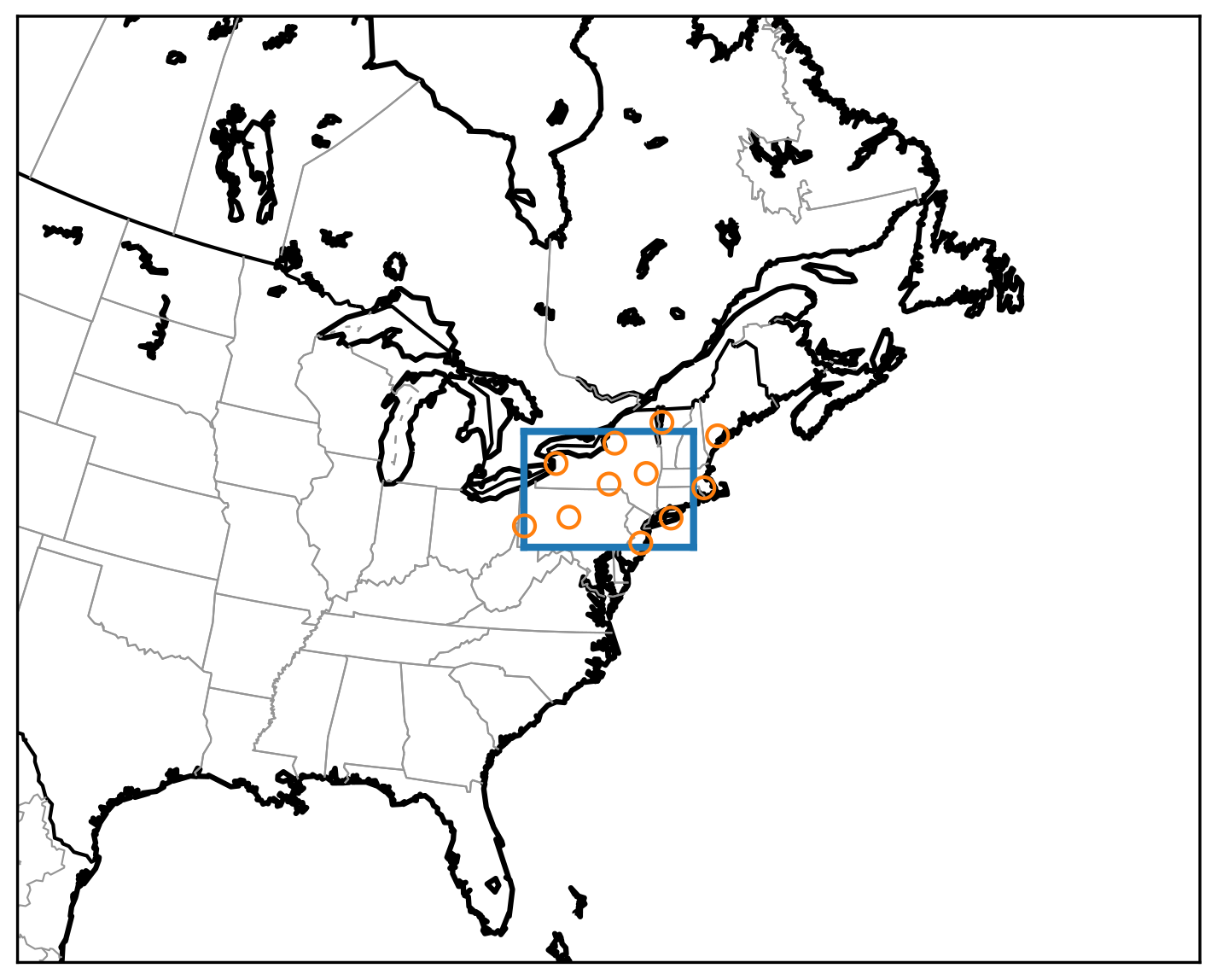
Figure 1 The study area in eastern North America. The blue rectangle indicates the area (720 km × 490 km), while the orange circles mark the locations of the NEXRAD radars.

The area is centered on the states of New York and Pennsylvania and also covers parts of the states of Connecticut, Massachusetts, New Hampshire, New Jersey, Rhode Island and Vermont, as well as a region of the Atlantic Ocean and a part of the Canadian province of Ontario. Although this region is not as convectively active as, for example, the US Great Plains or the Southeastern US, we chose it because it still experiences considerable thunderstorm activity and the hazard profile of these storms is similar to those in Central Europe: tornadoes are relatively uncommon, and the hazards consist mostly of hail, lightning, wind gusts and heavy precipitation (Kelly et al., 1985; Changnon, 1993; Yeung et al., 2015). The latitude of the region is also similar to that of Central and Southern Europe, and consequently the solar radiation profiles and the viewing angles of satellite instruments in geostationary orbit are similar. The main difference between this region and Central Europe is the topography: much of Central Europe is characterized by the Alps, while our study area is generally smoother and most of the variation in elevation is due to the less-prominent Appalachian mountain range.

We collected data from data archives for the period ranging from April to September 2020, with a time resolution of up to 5 min, depending on the source. The length of the study period and the size of the area were determined as a compromise between gathering an extensive dataset with a large number of samples and keeping the amount of data (already around 7 TB of raw data) that needed to be downloaded and processed manageable.

2.2 Data sources

Since the objective of the study was to investigate the utility of different types of data for nowcasting severe thunderstorms, we selected multiple qualitatively different data sources for analysis. In order to constrain the complexity of the study, we tried to avoid unnecessary overlap between the sources; thus, for example, we did not attempt to use similar data from multiple satellites, nor did we obtain ground-based lightning data, as they were already available from a satellite source. Moreover, in order to avoid the complications of data intermittency, we preferred to focus on data sources that are regularly available and avoid sources such as low-Earth-orbiting satellites that typically pass over a given area only 1–2 times per day. The final dataset includes data from a ground-based operational radar network, multispectral imagery and lightning data from a geostationary satellite, and NWP and DEM data. The details needed to obtain the data can be found under “Code and data availability” at the end of the article. The data sources are described in more detail in the following sections.

2.2.1 Radar data: NEXRAD

The Next-Generation Radar (NEXRAD; Heiss et al., 1990) network is the US operational radar network operated by the National Weather Service (NWS). It consists of S-band Doppler weather radars that cover most of the continental US as well as many other regions of the country. NEXRAD observations from multiple radars are processed by the National Severe Storms Laboratory (NSSL) into composite products using the Multi-Radar/Multi-Sensor System (MRMS; Zhang et al., 2016; Smith et al., 2016). Unfortunately, the MRMS data are currently only available in near-real time and are not publicly archived for more than 24 h. Therefore, we needed to process the data from individual radars – whose data are publicly archived in the long term – into a composite ourselves; the PyART library (Helmus and Collis, 2016) was used for this purpose. Although this solution has the drawback that we cannot expect to match the quality of a well-developed composite product within this study, it has an advantage in that using the full three-dimensional measured radar observations allows us to calculate any radar variable rather than just those available from the MRMS. In this work, we derived the column maximum reflectivity (MAXZ), the echo top heights at threshold reflectivities of 25, 35 and 45 dBZ, as well as the vertically integrated liquid (VIL), calculated as

$$\begin{array}{}\text{(1)}& \mathrm{VIL}=\mathrm{3.44}\times {\mathrm{10}}^{-\mathrm{6}}{Z}^{\mathrm{4}/\mathrm{7}},\end{array}$$

where Z is the radar reflectivity given in mm⁻⁶ m⁻³ (i.e., $Z={\mathrm{10}}^{Z_{\mathrm{dB}}/\mathrm{10}}$ for Z_dB in dBZ units) and VIL is in units kg m⁻² (Greene and Clark, 1972). The radar data have a time resolution of 5 min.

Radars were selected such that good data coverage was achieved throughout the study area. The parts of the area that are over ocean and in Canada are within the range of the selected radars, and the entire region is covered with a minimum beam altitude of at most 6000 ft (1800 m), and less than 3000 ft (900 m) across most of the region. NEXRAD radars operate using rather shallow scan elevation angles of 0.5–19.5^∘, and consequently each individual radar is blind to the region of the atmosphere directly above it. This gap must be filled with nearby radars, and therefore we also selected some radars outside the study area in order to ensure adequate 3D data availability within the area. The radars used for the study are listed in Table B1, and their locations are also shown as orange circles in Fig. 1.

2.2.2 Satellite imagery: GOES ABI

GOES-16 is a new-generation geostationary satellite with advanced instruments for weather observations (Sullivan, 2020). The primary GOES-16 instrument used in this study is the Advanced Baseline Imager (ABI), which includes 16 bands with wavelengths ranging from 470 nm (visible) to 13.3 µm (thermal infrared) and resolutions ranging from 0.5 to 2 km per pixel in optimal viewing conditions. GOES-16 is located over the Equator at 75.2^∘ W, a longitude near the middle of our study area. The ABI provides a full-disk scan, a variable region of interest (used for hurricanes, for example), and a scan covering only the contiguous US (CONUS) region. For this study, we use the CONUS scan, which is available with a time resolution of 5 min.

We downloaded the level 1 (L1) data (given as the reflectance or brightness temperature) for the GOES-16 ABI channels (Schmit and Gunshor, 2020) as well as the level 2 (L2) cloud products of cloud top height, cloud top pressure and cloud optical depth (Heidinger et al., 2020) and the derived stability indices (DSI) product (Li et al., 2020), which includes retrievals of variables such as the convective available potential energy (CAPE). We would have preferred to use the cloud-top temperature product as well, but it is available only as a full-disk product, not separately for the CONUS region. Consequently, we omitted the cloud-top temperature because the inferior time resolution (10 min) of the full-disk product would have caused compatibility problems. We also computed the differences of various L1 channels (listed in Table B3) in order to provide better features; see, for example, Mecikalski et al. (2010) for interpretations of the channel differences from geostationary visible/infrared imagers. The data were projected to our study grid with the PyTroll libraries (Raspaud et al., 2018) and corrected for parallax shift using the L2 cloud top height product to determine the appropriate correction.

2.2.3 Lightning data: GOES GLM

The GOES-16 satellite is also equipped with the Geostationary Lightning Mapper (GLM), which detects lightning strikes (Rudlosky et al., 2020). The GLM L2 data consists of the coordinates and properties, such as energy, of individual strikes. Each strike consists of multiple lightning “events,” which are pixel-level detections of lightning; a set of adjacent and simultaneous events is interpreted as a strike. The coordinates and properties of the events are also provided, thus providing information about the spatial extent of each lightning strike.

We projected the data on the lightning strikes and events, as well as their energies, to the common grid. The original GLM files contain 20 s of data each, but the files were aggregated such that we created derived products with 5 min time resolution. The GLM L2 data are provided with parallax correction already performed, obviating the need for this step.

2.2.4 Numerical weather prediction: ECMWF

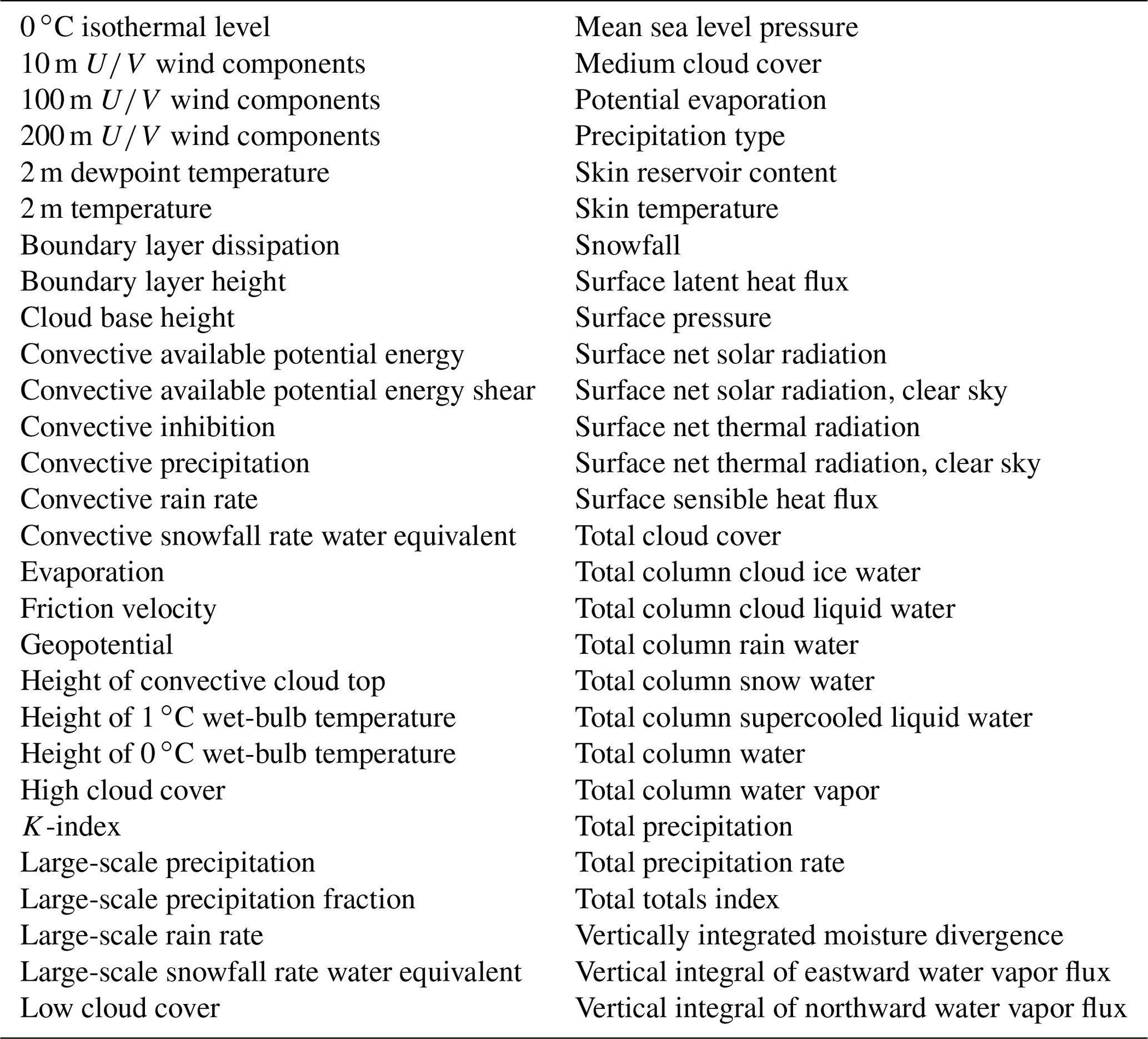
We provide the nowcasting system with information about the state of the atmosphere in the study area using the NWP products from the integrated forecast system (IFS) of the European Center for Medium-Range Weather Forecasting (ECMWF). We chose to use the global IFS rather than a local-area modeling system as our NWP data source because, unlike the satellite and radar data, it is not limited to a particular region, and we expected this to facilitate the adaptation of our methodology and results to Europe and other regions beyond the current study area later. We obtained a collection of 59 different variables provided by ECMWF; the variables are listed in Table B5.

We use the ECMWF archived forecast product rather than the analysis product in order to only use data that would be available to an operational nowcasting system. We downloaded the ECMWF forecasts at intervals of 12 h in forecast time, and the data in the forecasts have a resolution of 1 h. To each 5 min time step in our common spatiotemporal framework, we assigned the closest 1 h time step from the most recently issued forecast. ECMWF provides the data on a latitude–longitude grid; we used the PyTroll tools to project them onto our study grid.

2.2.5 Digital elevation model: ASTER

Orography can affect the development of convective storms. In order to enable the nowcasting system to exploit information about the elevation and morphology of the terrain, we obtained the Advanced Spaceborne Thermal Emission and Reflection Radiometer (ASTER) global DEM version 3 (Abrams et al., 2020). The resolution of the ASTER DEM is 30 m (the data are provided at a resolution of 1 arcsec), much finer than our grid pixel size of 1 km. This allows the computation of subpixel properties of the elevation for each grid point. We computed the mean elevation, the elevation gradients and the surface roughness, defined as the root-mean-square (RMS) deviation from the mean, for each pixel in our grid. As a combined variable, we also computed the upslope flow s, defined as the dot product of the elevation gradient and the flow velocity:

$$\begin{array}{}\text{(2)}& s=\mathrm{\nabla }h\cdot v,\end{array}$$

where h is the elevation and v is the flow velocity, which in this case is derived from the radar motion vectors. A positive s indicates that the air flows predominantly uphill, while a negative s corresponds to downhill flow. When we discuss the importance of data sources later, in Sect. 4.2 and 4.3, we consider the information content of the upslope flow to be one of the DEM variables.

3 Methods

3.1 Data processing

In order to keep the conclusions of the study general and applicable to different operational environments, general and widely available methods, rather than a particular operational nowcasting system, were used in the data processing workflow applied in this study. This starts with the identification of thunderstorm centers in the MAXZ field. The motion of these centers is then tracked backward and forward in time in a Lagrangian framework by integrating the velocity field obtained with the optical flow method. Once the motion of the center has been estimated, features from different data sources and variables are extracted from the neighborhood of the center at each time step. These features are collected in the ML dataset used to train a gradient-boosting model. Below, we describe each step of the workflow in more detail.

3.1.1 Extraction of storm centers and tracks

After processing the data into a single grid as described in Sect. 2.2, we identified regions of active thunderstorms in the data, based on the observed radar reflectivity. For each 5 min time step in the data, we located centers of convective activity using the following procedure:

1. Start with an empty list of storm centers.

2. Find the pixel with the highest MAXZ, denoted p_maxZ.

3. If the MAXZ at p_maxZ is at least 37 dBZ:

   • Add p_maxZ to the list of storm centers.

   • Identify the 25 km diameter circular area surrounding p_maxZ and exclude the pixels in it from the rest of the search.

   • Restart the search from step 2.

   Otherwise, end the search.

Thus, storms were identified as regions of high radar reflectivity. We chose the 37 dBZ threshold, which corresponds to a convective precipitation rate of approximately 8 mm h⁻¹, following several previous studies in which thunderstorms were identified using radar reflectivity thresholds of 30–40 dBZ (Marshall and Radhakant, 1978; Wilson and Mueller, 1993; Roberts and Rutledge, 2003; Mueller et al., 2003; Hering et al., 2004; Kober and Tafferner, 2009). To prevent radar artifacts from being identified as storms, we discarded centers that had a valid MAXZ in fewer than one-third of the pixels in the surrounding 25 km circle.

Once the centers had been identified, we tracked their movement in the domain so that the temporal evolution of the storm was separated from its movement. To estimate the motion, we computed the motion vectors of the reflectivity using the autocorrelation-based optical flow method implemented in the PySteps package (Pulkkinen et al., 2019). This method yields a single motion vector; to allow the motion vector field to vary spatially, we computed a motion vector in this manner for each point in a square grid with a spacing of 97 pixels, using the 200×200 pixel MAXZ neighborhood of each grid point to compute the vector using the autocorrelation-based method. Once computed in this fashion, the motion vectors were then interpolated to the storm centers. This method produces motion fields with very smooth gradients and is likely to fail to produce the correct motion for regions with high wind shear. Although more advanced methods are available in PySteps, we found these to be more prone to producing artifacts. The procedure described above is more robust, so we found it to be more suitable for the task required in this study: the automated analysis of tens of thousands of samples.

For each center, we estimated the past location of the corresponding air parcel by backward integrating the motion vectors using Heun's method (also known as the improved Euler's method; Süli and Mayers, 2003). At each time step, the advected center may be adjusted by up to 2 pixels to align it at the maximum MAXZ in the neighborhood (we found that 2 pixels was sufficient, and that larger adjustments sometimes caused the tracking to drift to the wrong storm center). For future motion, only the data that would be available in a real-time nowcasting scenario was used, and therefore we computed the future tracks using the last available motion vectors at the reference time. Both the past and the future tracks were computed for 60 min from the reference time. Any tracks that extended out of the study area were discarded. An example of centers and tracks extracted in this manner is shown in Fig. 2.

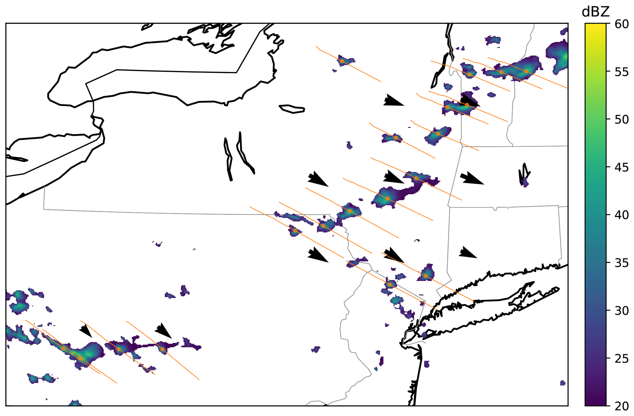
Figure 2 An example of the extracted centers at time t=0 (orange circles) and tracks from t−60 to t+60 min (orange lines). MAXZ in dBZ is shown in the colored map, with coastlines and state borders shown in the background.

The storm identification and tracking scheme was implemented with the objectives of robustness and suitability for ML. Therefore, we opted not to use, for instance, the thunderstorm radar tracking (TRT) cell identification method (Hering et al., 2004, 2005, 2006), which produces variable-sized storm cells, thus complicating analysis. Our scheme approximates the tracking of storm centers but may not always perfectly correspond to it. Therefore, one can state the objective of the ML prediction task more precisely as follows: given the Lagrangian history of a storm centerpoint selected based on a 37 dBZ reflectivity threshold, predict its future Lagrangian evolution.

3.1.2 Feature extraction

The evolution of a storm over time is described by the changes in the variables in the circular neighborhood of the center. For each variable derived from the data sources described in Sect. 2.2, we extracted the neighborhood mean, the standard deviation and the 10th and 90th percentiles. The percentiles are intended as a soft minimum and a soft maximum and are less sensitive to outliers compared to the exact minimum and maximum. For Boolean variables such as the occurrence of a lightning event, we also computed binary features that were 1 if the variable was true at any pixel in the neighborhood or 0 otherwise.

3.1.3 Datasets

The final dataset collected from the entire study period and study area comprises 87 626 samples that describe the history and future of the detected storm centers. We divided the samples into a training set that was used to train the ML algorithm, a validation set that was used to evaluate the generalization ability during training and a test set that was used for final evaluation. We found that simply sampling these sets randomly from the data made the training prone to overfitting because storm tracks found at a similar time and location had similar evolutions and thus were not independent samples. In order to improve the independence of the training, validation and testing sets, we determined these sets such that the data from each day (00:00–24:00 UTC) were assigned entirely to only one of these sets, mostly eliminating the overlap between them. We sampled the days randomly until at least 10 % of the data were in the validation set and at least another 10 % were in the test set, and assigned the remaining data to the training set. The final datasets were made up of 69 594 training samples, 9160 validation samples and 8872 testing samples.

3.2 Prediction tasks

The predictands (i.e., the targets of the ML prediction) evaluated in this study were selected based on their relevance for thunderstorm hazard prediction. We examined qualitatively different predictands in order to assess the differences in the contributions of various data sources to the prediction performance.

The first prediction task we defined was the nowcasting of the evolution of the column maximum reflectivity on the storm track. This variable is highly indicative of thunderstorm development and can function as an indicator of heavy precipitation and hail. In particular, the radar reflectivity Z can be approximately related to the rain rate R by a relation of the form Z=aR^b, where a and b are empirically determined constants. Hereafter, we refer to the task of predicting the evolution of the column maximum reflectivity as MAXZ. We examined the prediction performance for lead times of between 5 and 60 min.

Another important thunderstorm hazard that we were able to quantify using the available dataset was the occurrence of lightning. We used the GLM measurements to identify lightning, and approached lightning prediction as a binary task of predicting whether or not lightning will be present in the 25 km diameter neighborhood of the storm center during a given time period. We refer to this task as LIGHTNING-OCC.

For hail, we did not have direct observations of its occurrence. However, the presence of hail has been found to be well indicated by the height difference between the radar 45 dBZ echo top and the freezing height (Waldvogel et al., 1979; Foote et al., 2005; Barras et al., 2019). Since the freezing level is obtained from NWP data, the principal task is to predict the echo top height. This, of course, is dependent on a 45 dBZ reflectivity being present in the vertical column. Thus, we divided this task into two components: predicting whether a 45 dBZ echo top will be present (ECHO45-OCC) and, in cases where it was present, predicting its height (ECHO45-HT). In an operational setting, this model could be used by first evaluating ECHO45-OCC; if it predicted that a 45 dBZ reflectivity would occur, ECHO45-HT would then be predicted and the freezing level would be subtracted from it in order to calculate the hail probability.

3.3 Machine learning: gradient tree boosting

For the ML prediction, we used gradient boosting (GB) to learn the relationship between the features and the prediction targets. GB is a ML technique that uses decision trees, with trees trained iteratively such that each successive tree corrects the errors of the previous trees. The decision trees are regularized using several techniques in order to prevent overfitting. A review of GB methods can be found in Natekin and Knoll (2013).

One particular advantage of GB for our study is that it allows the importance of the various input features to be quantified. Thus, it is well suited to our aim of assessing the value of different data sources and variables for the prediction of thunderstorm hazards. The results can later be used to guide the selection of appropriate features for different ML methods such as deep learning, where the feature importance is less straightforward to derive.

We used the open-source LightGBM implementation of the GB algorithm (Ke et al., 2017) as our ML framework. LightGBM is designed to be computationally efficient and has a reduced memory footprint, facilitating the analysis of large datasets.

3.4 Training

We tuned the GB training for each of the various prediction tasks. As described in Sect. 3.2, the learning tasks can be broadly divided into two categories: regression tasks and binary classification tasks. In regression tasks, the objective is to predict the future value of a variable that can be any real number; in binary classification tasks, the objective is to predict the probability of an event occurring.

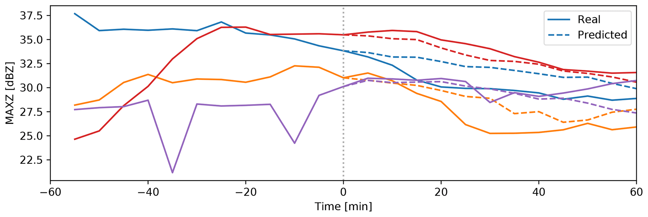
Figure 3 Examples of the prediction of MAXZ. The figure shows the curves of observed and predicted MAXZ (the mean over the 25 km diameter region of interest) for four different tracked centers. The solid lines show the development of MAXZ, while the dashed lines show the predictions after t=0.

After comparing the performance and robustness of the mean square error (MSE) and mean absolute error (MAE), we decided to use MAE as the training objective function for regression tasks, as it tended to give slightly better results with the validation set, with less overfitting. Indeed, when the model was trained with MAE loss, it achieved better MSE in the validation set than an equivalent model trained with MSE loss. Willmott and Matsuura (2005) and Chai and Draxler (2014), among others, have discussed the relative merits of MAE and MSE in the geoscientific context. We also found that, compared to training the GB model for the target variable directly, we could achieve superior training performance by first subtracting the bias-corrected persistence prediction (discussed in more detail in Sect. 4.1) and then training the GB model to predict the residual. Binary tasks were trained using the cross entropy as a cost function.

All tasks were trained using early stopping based on the validation dataset. That is, the training proceeds as long as the training metric keeps improving not only in the training set but also in the validation set, which is not used for training. The early stop limits the overfitting of the GB model.

The performance with the validation dataset was also used to tune the hyperparameters of the GB model, most importantly the depth of the trees, the number of leaf nodes, the learning rate and various regularization parameters. Although we were able to achieve some improvements by fine-tuning these parameters, the performance on the validation set was not particularly sensitive to changes over a reasonable range of parameters. As the principal goal of this study was not to strictly optimize the performance of the predictions but rather to assess the importance of the various data sources, we considered the hyperparameter tuning to be of secondary importance in this context and were content to use hyperparameters that produce reasonable results after an informal manual search of the parameter space.

Using the default hyperparameters, approximately 60 min were required on a modern computer with 16 central processing unit (CPU) cores to train the all GB models: 12 models corresponding to different time steps of the MAXZ prediction and two models (0–30 and 30–60 min) for each of the LIGHTNING-OCC, ECHO45-OCC and ECHO-45. Thus, one model took approximately 3 min to train. Evaluating all of the above-mentioned models for the entire testing dataset of 8872 samples required a total of 6 s on the same hardware; this is equivalent to 35 µs for one sample and one model.

4 Results and discussion

The results of the ML experiments are reported and discussed in the sections below. First, in Sect. 4.1 we give a general analysis of the prediction performance. Then we assess the importance of different features and data sources using the GB feature importance (Sect. 4.2) and data exclusion analysis (Sect. 4.3). All reported results are for the test dataset unless otherwise mentioned.

4.1 Prediction performance

Before evaluating the importance of the various data sources, we quantify the performance of the models in the case where all data sources described in Sect. 2.2 are available.

Figure 3 shows examples of the real and predicted time series for MAXZ. We note that, in this figure, the MAXZ at t=0 may be less than the 37 dBZ threshold because the MAXZ shown is the mean over the 25 km diameter region of interest, while a MAXZ exceeding 37 dBZ in a single pixel is enough for a case to be selected. Meanwhile, Fig. 4 shows the error, averaged over all events and data points, of the MAXZ predictand as a function of the lead time t. In order to provide a more concrete error figure, we also show the corresponding relative error in the rain rate estimated using the relation Z=300R^1.4, where Z is the reflectivity on the linear scale, derived for convective precipitation and frequently used with NEXRAD (e.g., Martner et al., 2008). As a baseline prediction, we use the persistence assumption in a Lagrangian framework; that is, it is assumed that the variable will remain the same as it was at time t=0. We found that the persistence assumption is biased: the MAXZ at t>0 is, on average, lower than that at t=0; this can also be seen in most of the examples in Fig. 3. This reflectivity bias has two sources: first, sampling bias, which occurs because we select centers of intensive thunderstorms with MAXZ>37 dBZ; and second, drifting of the thunderstorm track from the actual center of the storm due to inaccuracies in the tracking procedure. The bias is small at short lead times and reaches 3.5 dBZ at t=60 min.

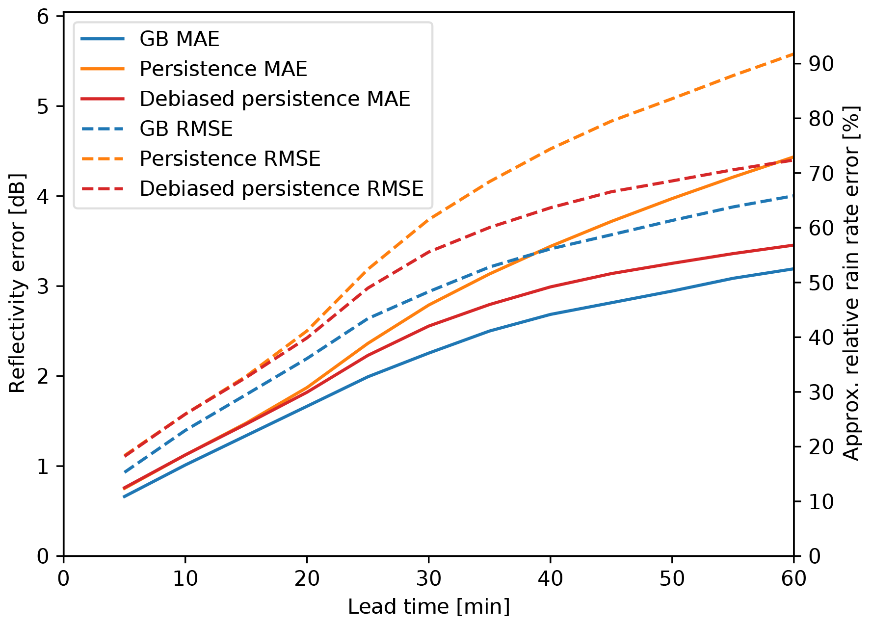
Figure 4 Errors (in dBZ) of the prediction of MAXZ as a function of lead time, obtained using all the available data. The solid lines show the mean absolute error (MAE), while the dashed lines show the root-mean-square error (RMSE) as shown on the scale on the left. The scale on the right shows the logarithmic reflectivity error converted to the relative error in rain rate R. The blue lines show the result from the GB tree, the orange lines show the Lagrangian persistence assumption and the red lines show the bias-corrected Lagrangian persistence.

We can considerably reduce the error of the persistence assumption by correcting for this bias. In contrast, it is rather difficult to improve from the bias-corrected persistence assumption using the GB model, even if we train the GB model on its residual. In Fig. 4, it is apparent that the bias correction improves the MAE by approximately 1.2 dB at t=60 min, while the GB model only gives a further 0.3 dB of improvement. Nevertheless, the improvement gained with the ML prediction is consistent and increases with longer lead times.

For the lightning prediction, the model has an error rate of 8.1 % for LIGHTNING-OCC in the 0–30 min time period and 14.3 % for the 30–60 min period. We can compare these numbers to the climatological occurrence, which would be the error rate of a prediction that lightning never occurs – or conversely, the climatological nonoccurrence would be the error rate of a prediction that it always occurs. The climatological occurrence of lightning in the data is 40.7 % for 0–30 min and 29.2 % for 30–60 min in the test dataset (the difference between these is likely due to the same bias that we discussed in the context of MAXZ above). These results suggest that the nowcasting framework developed here could potentially be adapted to operational lightning nowcasting. Full confusion matrices are shown in Fig. 5a and b.

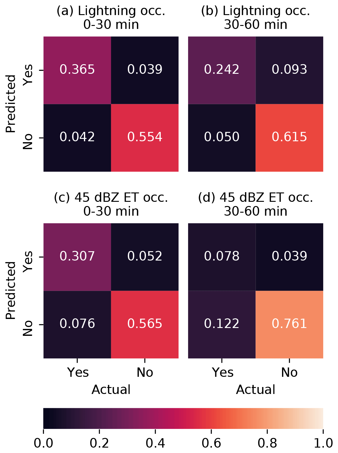
Figure 5 Confusion matrices for (a, b) the LIGHTNING-OCC prediction task and (c, d) the ECHO45-OCC task.

For the presence of the 45 dBZ echo (ECHO45-OCC), we find error rates of 12.7 % for the 0–30 min range and 16.5 % for the 30–60 min range. The corresponding climatological occurrences in the test set are 38.3 % for 0–30 min and 20.0 % for the 30–60 min range. Thus, we achieve a considerable improvement with the ML approach for the near-term prediction but a far more marginal one for the longer term, which implies a more limited ability to predict hail, and other features associated with the 45 dBZ echo top, using the approach applied in this study at lead times over 30 min. The confusion matrices for ECHO45-OCC can be found in Fig. 5c and d. In the subset of the test dataset where the 45 dBZ echo is present, the height of the 45 dBZ echo is predicted with a MAE of 693 m for 0–30 min and 841 m for 30–60 min. According to the formula in Foote et al. (2005) for the probability of hail (POH), these correspond to roughly 16 and 19 percentage-point errors in POH, respectively. Meanwhile, the standard deviations of ECHO45-HT in the test set are 1365 m for 0–30 min and 1404 m for 30–60 min.

4.2 Feature importance

The importances of features to the GB model can be extracted from the LightGBM library after training. In this section, we show the “gain” of various features, i.e., the total reduction in the training loss function attributable to that feature. For clarity and brevity of presentation, we sum the contributions from different feature types (e.g., mean, standard deviation) and different time steps. We also separately consider the total contribution from all features of a given data source, which can give a clearer impression of the total importance of a source that includes a large number of correlated features.

Figures 6 and 7 show the importances of the various predictors and data sources (e.g., ABI, NWP model or radar) for each of the ML objectives defined in Sect. 3.2. In Fig. 6, we show the feature and source importances of the MAXZ and LIGHTNING-OCC objectives, while Fig. 7 displays the same for ECHO45-OCC and ECHO45-HT.

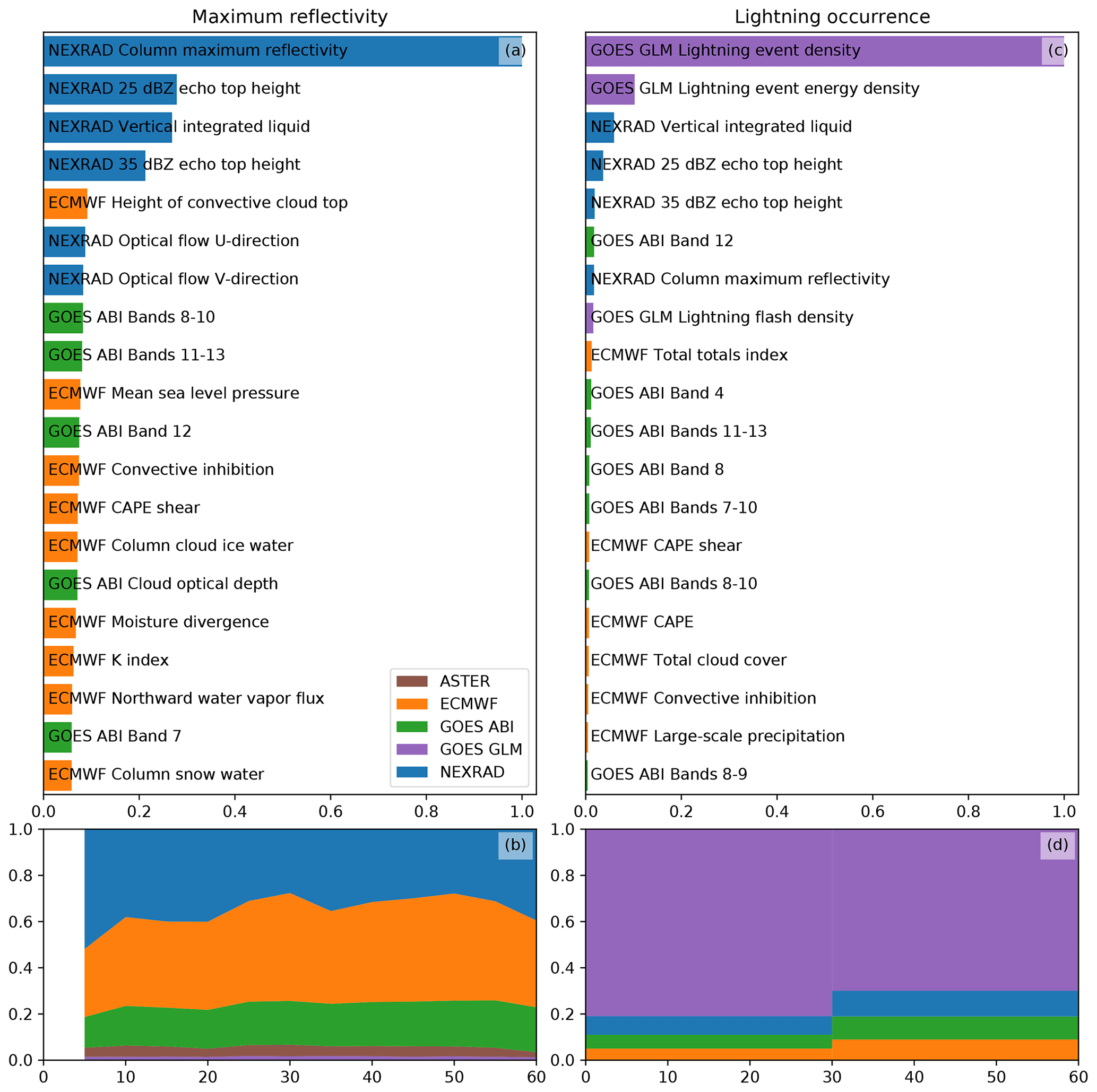
Figure 6 The importances of the various features and data sources for the MAXZ (a, b) and LIGHTNING-OCC (c, d) predictands according to LightGBM. The top panels show the 20 most important source variables for each predictand. The importances have been summed from all features and time steps and normalized such that the most important variable is scaled to 1. The bottom panels show the total importances of the various data sources as a function of lead time (in panel b) or the prediction time range (in panel d).

Figure 7 As Fig. 6, but for the ECHO45-OCC (a, b) and ECHO45-HT (c, d) predictands.

The statistics of feature importance for nowcasting MAXZ, as shown in Fig. 6a, demonstrate that the most important features for predicting this target variable come from the NEXRAD radar data. The most significant feature is the column maximum reflectivity – the same variable that is being predicted – but the other radar variables also seem to be utilized. The importances grouped by data source, as displayed in Fig. 6b, show a slightly different view, as in this case the NWP data are of similar importance to the radar. The reason for the apparent discrepancy between the importances of individual features and the total source importance is that contribution of the NWP data is divided over a large number of variables that are correlated to varying degrees. Because of the correlations, the contributions from individual variables appear small, as the GB model splits the gain between the correlated variables, but the contributions combine to give an importance comparable to the radar variables when summed together. Figure 6b shows some variation in the relative importances of the radar and NWP data between time steps, which we consider to be most likely mere random noise; as the different time steps are predicted by different, independently trained models, they may end up with slightly different values for the feature importance. In general, the importance of the NWP data tends to increase slightly with longer lead times, as was also found in earlier nowcasting studies (e.g., Kober et al., 2012). The GOES-16 ABI data are also utilized to a significant degree, while the GLM and ASTER data contribute to a lesser extent.

The feature and source importances for LIGHTNING-OCC, as shown in Fig. 6c and d, are dominated by contributions of the GLM lightning data. This is largely because a region that is already producing lightning is likely to continue to do so in the future, thus providing a reliable predictor, but past occurrence can also indicate temporal tendencies in lightning activity. The NEXRAD, ABI and ECMWF data are considered to be approximately equally important, with their total importance (Fig. 6d) relative to GLM increasing with longer lead times.

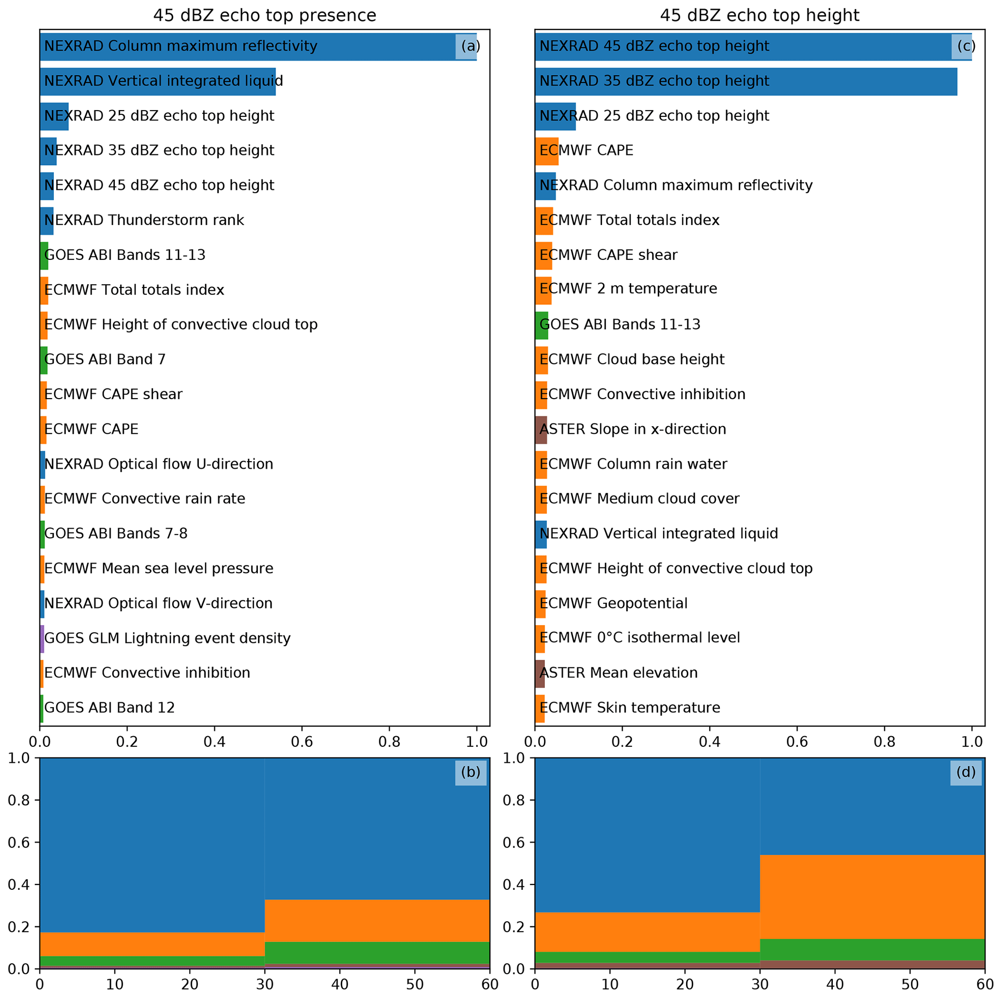
Figure 7 shows the feature importances for ECHO45-OCC and ECHO45-HT. Similar to the nowcasting of MAXZ, the most important features are from the NEXRAD radar data. Again, this is not unexpected given that the target variables are defined using the radar. The ECMWF and ABI data contribute less to the prediction of the echo top than to the prediction of MAXZ. According to this analysis, the GLM data are hardly used, while the ASTER DEM data seem to provide a small contribution to the prediction of echo top height. However, as we shall discuss in Sect. 4.3, GLM actually provides useful data in the absence of other predictors, while the importance of the DEM may be due to overfitting.

4.3 Exclusion studies

An alternative way to assess the importance of various data sources is to remove one or more data sources from the training data, retrain the model, and evaluate the change in prediction performance. This approach may give later studies a clearer picture of the value of various data sources in thunderstorm nowcasting applications. Unlike the feature importance, such an exclusion study also allows the use of the testing set for evaluation, showing which variables are important in practice and allowing us to better distinguish generalizing learning ability from overfitting. The results of the exclusion experiments are shown in Fig. 8 (MAXZ and LIGHTNING-OCC) and Fig. 9 (ECHO45-OCC and ECHO45-HT). We also show the equivalent results for the training and validation datasets in Figs. A1–A4.

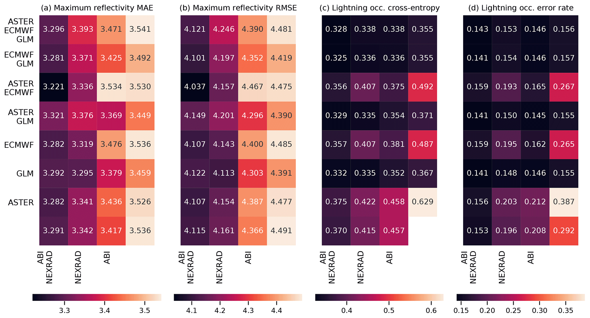
Figure 8 The results of exclusion experiments on the MAXZ and LIGHTNING-OCC predictands. Each square in panels (a)–(d) corresponds to a combination of data sources, which can be found by combining the sources listed for the row and the column. For example, the top left square of each panel shows the error metric obtained using all five data sources, while the second column of the second row shows the metric for ECMWF, GLM and NEXRAD data. The predictand and the error are shown on top of each panel; RMSE indicates the root-mean-square error and MAE the mean absolute error. In panels (a) and (b), the bottom right corner shows the result obtained with the bias-corrected persistence assumption (see Sect. 4.1), while in panel (d), the bottom right corner shows the baseline climatological occurrence. The results for LIGHTNING-OCC are shown for the 30–60 min time interval.

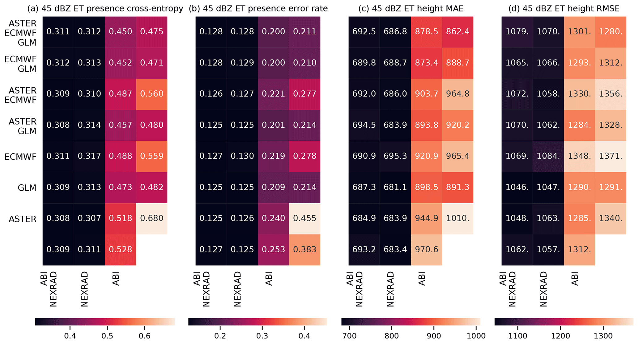
Figure 9 As Fig. 8, but for the ECHO45-OCC and ECHO45-HT predictands. In panel (b), the bottom right corner shows the climatological occurrence (unlike with MAXZ, we do not use the persistence assumption as a baseline for ECHO45-HT, and therefore nothing is shown in the bottom right corner of panels (c) and (d), in contrast to Fig. 8a and b). The results are shown for the 0–30 min time interval.

The results for the MAXZ predictand at 60 min lead time can be found in Fig. 8a and b. There is some noise in the results, so small differences in the metrics should not be overinterpreted, but certain general patterns are apparent. Most noticeably, the two leftmost columns, which correspond to models that have the NEXRAD radar data available, show consistently lower errors than the two columns on the right. The ABI data also have a positive effect, as can be seen by comparing the first column to the second, or the third to the fourth. Examining the differences between the rows, GLM data have a slight positive effect, especially when few other data sources are available, while it is difficult to discern any consistent effect from including the ECMWF data, and including the ASTER data sometimes even appears to make the metrics slightly worse. The latter result may be caused by the GB training process overfitting to the DEM features during training, degrading the results obtained during testing. Among the predictions obtained using only one data source, the one with NEXRAD data yields the best results and is almost as good as using all data sources together, the ABI and GLM data provide slight improvements over the baseline case (shown in the bottom right corner), while the model using only the NWP data from ECMWF yields results approximately equal to the persistence baseline. The latter result is quite surprising considering the large weight assigned to the ECMWF features in the feature importance analysis (Fig. 6a and b). For unclear reasons, the single best combination seems to be that which uses all data sources except GLM; we suspect that this result is merely coincidental and due to random variation because the results in Fig. 8a and b do not suggest that the GLM data are detrimental to prediction performance. The results for the training and validation sets (Appendix Figs. A1a, b and A3a, b) support this interpretation, since the best combination in the validation dataset is that of NEXRAD and GLM. More generally, the results for the training and validation datasets exhibit patterns similar to those in the test set, which suggests that while individual differences may be attributable to noise, the broader conclusions of the analysis are robust.

The metrics for LIGHTNING-OCC, shown in Fig. 8c and d for the 30–60 min time interval, also show a clear pattern. Here, the first, second, fourth and sixth rows, which correspond to the GLM data being available, show better metrics than the other rows. Indeed, prediction using only the GLM data performs very well, achieving an error rate of 15.5 %. However, it is interesting to note that good results can be obtained without the direct lightning data as well; for example, the error rate obtained using only the ABI and NEXRAD (15.3 %) data is better than the GLM-only error rate and only 1.2 percentage points worse than the best result (14.1 %). This shows that the feature importance analysis shown in Sect. 4.2 is only valid for a specific combination of predictors. When one data source is removed, the missing information can often be substituted by other data sources that were much less used in the case in which everything was available. In general, both the ABI and NEXRAD data improve the prediction results for LIGHTNING-OCC: the first column (with both ABI and NEXRAD available) has the best results overall, the comparison between the second (NEXRAD only) and the third (ABI only) is mixed, and the fourth (neither ABI nor NEXRAD available) has the worst results. The results obtained with the ECMWF data are rather odd. First, in contrast to the MAXZ prediction, the ECMWF data have some skill at predicting lightning on their own, as the ECMWF-only prediction has an error rate that is 2.7 percentage points better than the climatological average of 29.2 %. Second, prediction with both ECMWF and ABI performs 4.6 percentage points better than ABI-only prediction, but adding the ECMWF data to NEXRAD does not offer an improvement over the NEXRAD-only scores. This result may be simply noise, as in the validation dataset (Fig. A3d) the addition of ECMWF data also improves the results obtained with NEXRAD. The ASTER data do not add much information, and the ASTER-only prediction, with its 38.7 % error rate, actually performs worse than the climatology. This happens because the climatological occurrence in the training dataset, at 42.5 %, is coincidentally significantly higher than in the test dataset. The ASTER-only model is unable to generalize with the scarce data available to it, and only learns to roughly reproduce the climatological error rate in the training dataset, which leads to the overestimation of occurrence in the test set. Indeed, the degradation of the metrics with the addition of ASTER does not occur in the training and validation datasets.

For both ECHO45-OCC and ECHO45-HT (Fig. 9, shown for the 0–30 min interval), the clearest pattern is the importance of the radar data for prediction, which is consistent with the feature importance analysis. Indeed, as long as the NEXRAD data are available, the benefit of adding further data sources is negligible compared to the NEXRAD-only case (error rate of 12.5 %). However, without the NEXRAD data (e.g., in oceanic regions without radar coverage), the other data sources still provide meaningful improvements in ECHO45-OCC over the climatological occurrence of 38.3 %. For example, ABI alone achieves an error rate of 25.3 %, ECMWF alone yields 27.8 %, and GLM alone achieves 21.4 %, while these three sources together reach 20.0 %. Similar patterns are found in ECHO45-HT. These results further demonstrate that the benefits of features and data sources cannot be evaluated in isolation and depend on the other data sources used.

5 Conclusions

For machine-learning methods to be utilized effectively for thunderstorm nowcasting, it is necessary for the benefits of the various available data sources to be well understood and quantified. Large amounts of data that are potentially related to convective processes can be obtained from numerous sources, yet it is not always obvious how much benefit one should expect from adding an additional data source, and therefore additional complexity, to a ML model. This study provides guidance for future work to better select data sources for nowcasting particular thunderstorm hazards along predicted storm tracks. We obtained data from ground-based radar (NEXRAD), satellite spectrographic imagery (GOES-16 ABI), satellite-based lightning detection (GOES-16 GLM), a numerical weather prediction model (ECMWF IFS) and a digital elevation model (ASTER), for a total of over 100 input variables. We applied this data to nowcast variables related to precipitation, lightning and hail formation.

We have based our evaluation of the importance of various features on two complementary approaches: first, using the feature importance provided by the gradient-boosted tree algorithm, and second, retraining the GB algorithm repeatedly using different subsets of the input variables. Testing all possible combinations of input features would have quickly become implausible as the number of features increased, but grouping the features by data source allowed us to cover the most realistic situations of missing data, where an entire data source is unavailable due to either geographical limitations (for example, operational weather radar networks do not cover the oceans) or irregular data outages.

Each of the investigated data sources proved to be useful for predicting at least some of the target variables, except for the DEM, which provides no detectable benefit for any of the predictands. The radar variables are strong predictors for all predictands and are particularly dominant for the targets defined using the radar data. The satellite imagery from ABI provides moderate performance improvements to all predictands, though it is generally less significant than the radar data in this application. The GLM lightning data are highly useful for lightning prediction; for other targets, they provide more modest benefits, although they can still provide improvements to nowcasting performance, particularly when radar data are not available. More generally, the results confirm that satellite data can be used to provide ML-based nowcasts in areas without radar coverage, such as over the oceans and in less-developed regions lacking ground-based radar networks. Meanwhile, the ECMWF forecast data, despite being considered of some importance by the ML algorithm, do not benefit the nowcast according to the data exclusion analysis, as, for the lead times investigated here, the necessary information content is already contained in the other observations.

The results show that the feature importance from the GB algorithms may provide seemingly contradictory results compared to the more comprehensive analysis achieved by testing different combinations of features and evaluating the results. Although the two evaluation methods largely agreed on which data sources are the most important, some important differences emerged on closer inspection. This highlights the pitfalls of analyzing the importance of features and data sources in an ML setting when the data sources are partially redundant. A given feature may be beneficial when used alone, but virtually useless when used in conjunction with another, more powerful predictor. For instance, when trained for lightning prediction, the ML algorithm only gains a modest improvement (approximately 10 %) in the error rate from auxiliary data sources when direct lightning data are available, but when trained without lightning data, good prediction performance can still be achieved utilizing the other data sources. This has important implications for real-time nowcasting in time-critical applications such as aviation, as it indicates that ML-based nowcasting can be performed robustly when some input data are missing or delayed.

Based on the results, we conclude that investigators should be cautious with applying the brute-force strategy of providing ML algorithms with all the available data and letting the training process decide which data are useful. While this may sometimes reveal unexpectedly useful input variables, using data sources that contain little or no generalizable information may also expose the training process to the problem of overfitting, thus actually degrading the results. This can be mitigated by early stopping and by using hyperparameters designed to prevent overfitting, but it is better for both accuracy and training time to simply drop the counterproductive data sources.

Future work can take advantage of the results achieved in this study to build more accurate and efficient ML models for the nowcasting of the thunderstorm hazards of heavy precipitation, lightning and hail. It also allows the estimation of the degradation of the result if one observation system is missing. Nevertheless, this work is constrained to a particular set of data sources, a single study area and a specific ML method: the gradient-boosted tree. Although we have selected five commonly utilized data sources, all qualitatively different from each other, later work should extend the analysis to other data sources such as polar-orbiting satellites and ground-based lightning networks. Given suitable data sources, the methodology could also be extended to other hazards such as wind damage and tornado events. It may furthermore be interesting to investigate additional regions; for instance, the DEM data may be more significant in regions with higher mountains. With regard to alternative ML methods, the performance of neural networks should be evaluated in a future study, preferably using the same dataset to facilitate comparisons, as convolutional neural networks are expected to be able to better utilize spatial features such as the high-resolution imagery from the ABI instrument. Neural networks may also be able to utilize large numbers of samples and input variables better.

Appendix A: Exclusion studies on training and validation datasets

The exclusion analyses shown in Sect. 4.3 for the test dataset were also performed with the training and validation datasets. The results are shown in Figs. A1 and A2 for the training set and in Figs. A3 and A4 for the validation set.

Figure A1 As Fig. 8, but for the training dataset.

Figure A2 As Fig. 9, but for the training dataset.

Figure A3 As Fig. 8, but for the validation dataset.

Figure A4 As Fig. 9, but for the validation dataset.

Appendix B: Further information on the datasets

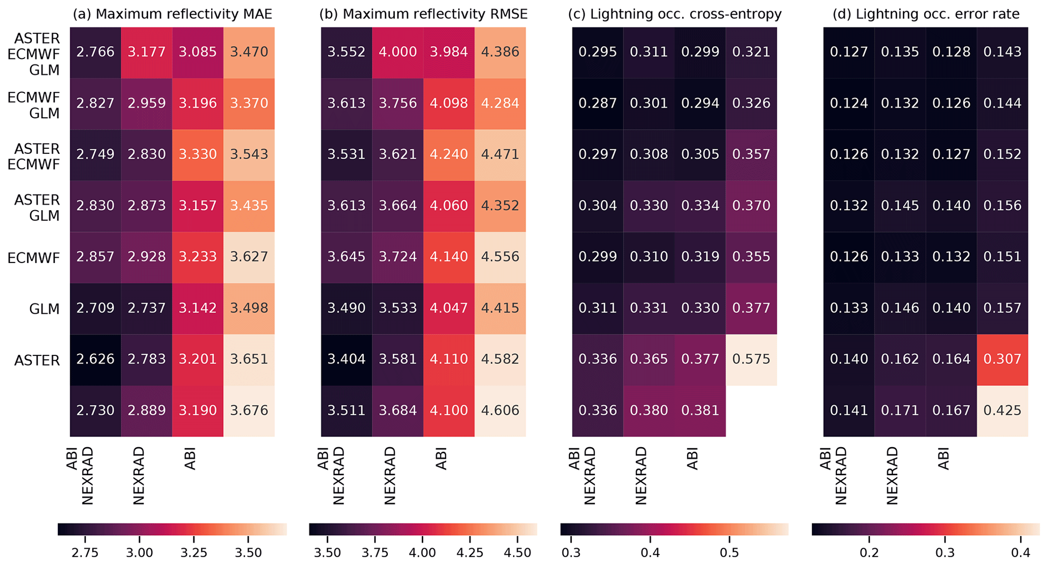
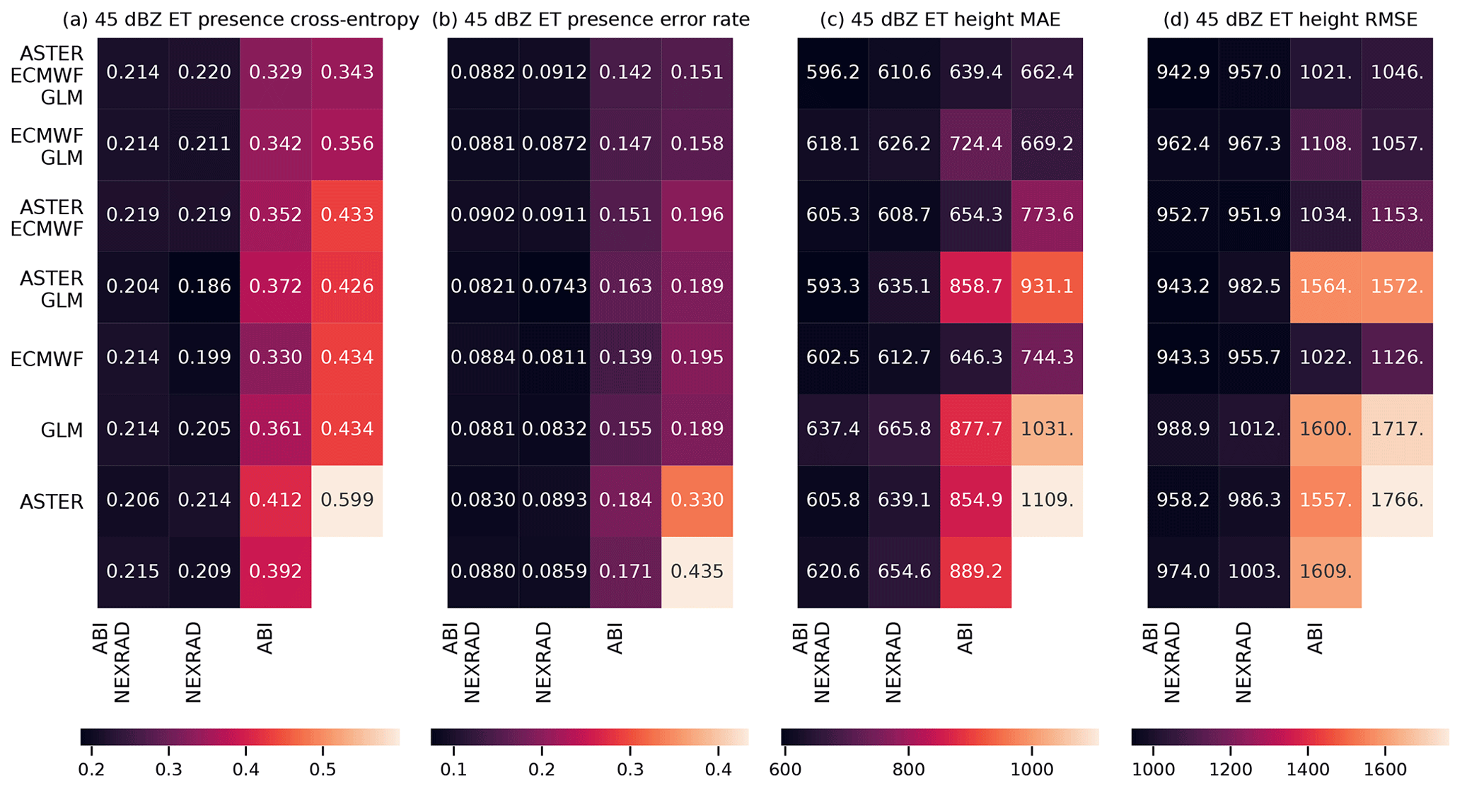
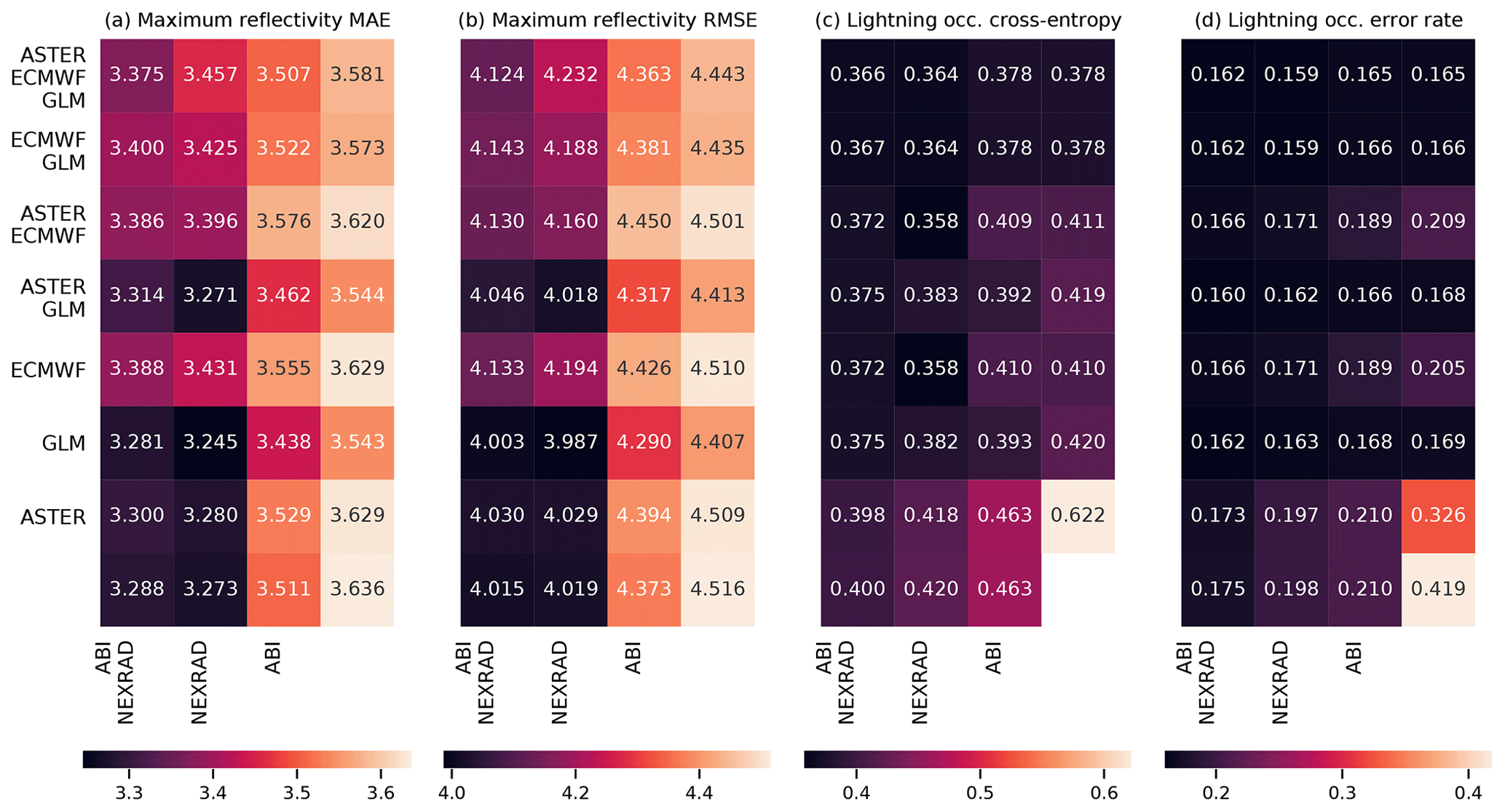
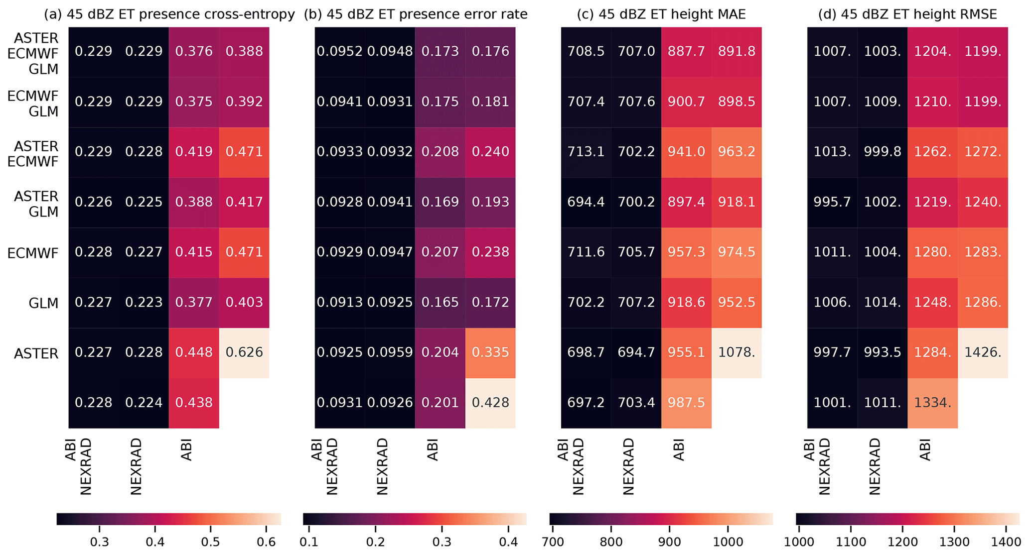
Table B1 lists the radars used to compile the NEXRAD dataset we used. Tables B2–B6 list the predictors from the various data sources that were used in this study.

Table B1 NEXRAD radars used to produce the dataset used in this study.

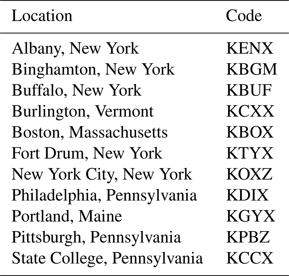
Table B2 Variables from the NEXRAD radar adopted in this study.

Table B3 Variables from the GOES-16 ABI instrument adopted in this study.

Table B4 Variables from the GOES-16 GLM instrument adopted in this study.

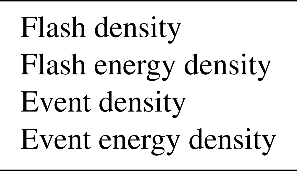
Table B5 Variables from the ECMWF model output adopted in this study.

Table B6 Variables from the ASTER DEM adopted in this study.