Temporal models for the occurrence of Etna eruptions and implications for hazard assessment

Mt. Etna volcanic activity is broadly divided into flank eruptions and summit paroxysms. Here, building on previously-available literature and data on the start time of these events, we collate two separate catalogs of the two activity types. Then we separately model their temporal occurrence. The catalog of flank eruptions, spanning the last 400 years, has been modelled by means of the most widely used renewal models, among which the best one (through Akaike Information Criterion) is the Brownian Passage Time. The catalog of summit paroxysms, covering the period 1986–2022, according to our cluster analysis is best characterized by 12 clusters of paroxysms. We separately analyze the inter-event times between onset times of successive clusters of paroxysms (Inter-Cluster inter-event times) and the inter-event times between successive paroxysms within clusters (Intra-Cluster inter-event times). Again, the Brownian Passage Time is the best-fitting model, obviously with very different parameters in the two cases. We test the best-fitting models by checking their ability to reproduce features of the real catalogs. Finally, we provide an example of how to use in practice such temporal models in the context of probabilistic hazard assessment, showing a possible use in the case of tephra fallout hazard from summit paroxysms. In particular, the proposed temporal model enables the assessment of probabilistic volcanic hazard for tephra fallout over different time windows accounting also for the uncertainty in the temporal occurrence of summit paroxysms.

1 Introduction

The temporal occurrence of volcanic events is one of the key ingredients to evaluate volcanic hazard and risk. In the literature, the statistical modelling of the temporal occurrence at a given volcano has been tackled with different models, fundamentally assuming eruptions as realizations of a point process in time, i.e., neglecting the duration of the eruption, as it is usually much shorter than the inter-event time (IET) between two successive eruptions. For a review of the use of temporal models in volcanology, we remand the reader to Sandri et al. (2021).

Mt. Etna in Sicily (Italy) is one of the most active volcanoes in the world. Its activity is mostly divided into summit and flank activity, characterized by different eruptive behaviour. Summit activity occurs from summit craters and it is mostly characterized by Strombolian activity and episodic lava fountains or paroxysms, often associated with lava emission (Guest and Murray, 1979; Branca and Del Carlo, 2005). Paroxysms are typically short-lived (up to several hours) and frequent episodes (on average 7 per year since 1986 CE), producing an eruptive plume that can reach 17–18 km a.s.l. (Corradini et al., 2018), with total erupted mass values up to ≈ 10¹⁰ kg (Scollo et al., 2013). In contrast, flank eruptions are more rare events (on average less than 2 events every 10 years, in the last 4 centuries), characterized by lava effusion often associated with explosive activity forming an ash plume, lasting from a few days to months (Guest and Murray, 1979; Branca and Del Carlo, 2005).

In this work we model the occurrence in time of summit paroxysms and flank eruptions separately, assuming they occur independently one type from the other. There are several reasons why we model separately the two types of event. First, from a phenomenological point of view, they have very different dynamics, explosivity, erupted magma and characteristic return time, somewhat implying that the processes leading to the two types of events are different. Second, from the point of view of the data, the temporal range covered by the complete part of their catalogs are very different. Flank eruptions, although much more rare than summit paroxysms, likely impact the towns and villages located on the volcano slopes through their lava flows and prolonged tephra emission, and leave a footprint in the geological record: this is why we can reasonably assume that the catalog for flank eruptions published by Branca and Del Carlo (2005) represents a complete list of this type of events since at least 1760 CE. Paroxysms, on the other hand, had little impact on economy and society until a century ago or so, when air and road traffic was not an issue. Furthermore, transient paroxysms may be missed by human eye in case of cloudy weather, and their footprint in terms of tephra layer at the ground is quickly removed or depleted by wind and rains. For all these reasons, the catalog of summit paroxysms at Etna can be reasonably considered complete since 1986 CE (Andronico et al., 2021), when the support from monitoring (seismic and remote) has become more and more effective in detecting and characterizing summit activity at Etna.

2 Data

2.1 Flank eruptions

We make use of the flank eruptive fissures dataset reconstructed in Proietti and Branca (2024) by selecting mapped lava flows in the last 4000 years from the Etna New Geological Map (Branca et al., 2011b), its subsequent updates (Branca and Vigliotti, 2015; Branca et al., 2015; Branca and Abate, 2019) and complementing papers on Etna activity (Behncke and Neri, 2005; Branca and Del Carlo, 2005). The flank eruptive fissures corresponding to reconstructed lava flows were then localised; in several cases, not a single fissure but a systems of fissures had fed the mapped lava flow, and it was catalogued as a single event in time for the purposes of the present paper. The historical eruptive fissures covered by the eruptions occurred after the 19th century were reconstructed and integrated by the geological map of (Branca et al., 2011a) with previous 1 : 50 000 cartographies compiled by Sartorius Von Waltershausen (1848–1861) and Romano et al. (1979), and maps of the 1971–1991 eruptions (Azzaro and Neri, 1992).

2.2 Summit paroxysms

Of the 259 paroxysmal eruptions from Mt. Etna between September 1986 and February 2022, 242 have been monitored. All of the paroxysmal eruptions originated from the summit craters: about 2 %, 2 %, 6 % and 90 % respectively from Bocca Nuova, North-East, Voragine and South-East craters. However, only around 160 events were observed by means of different sensors simultaneously, and subsequently characterized quantitatively. These eruptions have been extensively documented in the literature, typically with key eruption source parameters (ESPs) such as volcanic cloud height, start and end time of the paroxysmal activity, mass eruption rate and total erupted mass. Here we use the dataset compiled within PANACEA project, provided in the Supplement. The catalogue was assembled by merging previously published datasets from Andronico et al. (2021), Calvari et al. (2018), Calvari and Nunnari (2022) and Mereu et al. (2023) in terms of start and end time of the paroxysms, and complementing them with the information on summit paroxysms occurred up to February 2023 retrieved from the official bulletins and data from remote sensing systems. For the few events that overlap among the different sources, we prioritized data estimated directly derived from radar measurements (Mereu et al., 2023). When radar-derived information was unavailable, we used data from the literature, first from Calvari et al. (2018) and Calvari and Nunnari (2022), and subsequently, where necessary, from Andronico et al. (2021). This hierarchical selection strategy was adopted to standardize the dataset and to ensure rigorous quality control of the information included in the catalogue.

3 Methods for model setup and test

To model the temporal occurrence of flank and summit paroxysms separately, for each dataset first we compute Inter-Event Times (IETs) as the time intervals between the onset of two subsequent events. Due to the different features of the two datasets, mostly in terms of recurrence and clusterization, the methodology adopted to model time occurrence, and to test the model, is different. For flank eruptions, we first estimate the completeness date, defined as the time after which the eruption catalogue is assumed to be complete, i.e., no eruptions are considered to have been missed. This estimate is obtained under the assumption of stationarity. We then test the resulting catalogue for temporal independence (by means of the method reported in Bebbington, 2012), and clusterization (by means of the Coefficient of Variation, CV) of the IET data over the completeness time interval (see Table 1). For summit paroxysms, we assume that the catalogue is complete since its first event reported (due to the continuity of monitoring since 1986) and, as for the flank eruptions, we also test stationarity, independence and clusterization.

Table 1 Statistics on the datasets. Along the different rows we provide the following statistics, respectively: (1) mean annual rate of eruptions, (2) p-value of the stationarity test as in Bebbington (2012), (3) test on the independence of events (ρ is the Spearman correlation coefficient between pairs of successive IETs, as in Bebbington, 2012), (4) its p-value, and (5) CV (Coefficien of Variation). Different columns show these statistics for different catalogs: first column for flank eruptions since 1760 CE, and second for summit paroxysms.

3.1 Flank eruptions

We first identify the complete portion of catalogue by assuming stationarity and retaining only the most recent interval for which this hypothesis cannot be rejected. To do so, we consider only the eruptions after year 1000 CE (as can be seen in Fig. 1b in Sandri et al., 2024,  before year 1000 CE the rate of eruptions is clearly lower, likely due to evident incompleteness) and we run a change-point analysis to look for breaks-in-slope. We test that the portion of flank eruption dataset after the most recent change-point is stationary (and, in case, we take it for complete under our assumption) and composed by independent IET (see Bebbington, 2012). We check that there is no evidence of clustering by inspecting the CV (see Table 1). Thus, we model flank eruption temporal occurrence by testing six different renewal models most frequently used to describe IETs in volcanology (as in Sandri et al., 2021, Exponential, Weibull, Gamma, Brownian Passage Time, LogNormal, LogLogistic). We select the best model by means of the Akaike Information Criterion (AIC, Akaike, 1974) and its small-sample corrected version (AICc), searching a good compromise between model complexity (defined by the number of model parameters) and goodness of fit to the data (defined by the likelihood).

To test the preferred model, we use the bootstrapped Kolmogorov-Smirnoff's one-sample (KS1) test (Zeimbekakis et al., 2024), under the null hypothesis that the IETs for flank eruptions are a random sample generated by the preferred model. To do so, we generate 4000 synthetic catalogues of IETs from the preferred model, and for each of them we run the KS1 test. The 95 % confidence interval on the bootstrap KS1 test statistics provide bounds for the real test statistics not to reject the null hypothesis. We also account for the uncertainty on the best-estimate parameters of the preferred model. To do that we sample 350 values of the model's parameters within their uncertainty (considering their covariance, if there is more than 1 parameter, by sampling from a multivariate normal pdf), and run 350 KS1 tests.

3.2 Summit paroxysms

For the summit paroxysms, their CV (see Table 1) and their cumulative number in time (Fig. 3) shows a clear tendency to cluster, and thus we adopt the same procedure as in Sandri et al. (2021). In particular, we first objectively partition the dataset into clusters by applying a k-means clustering procedure, testing different values of k (from 1 to 25). We identify the best partition into $\widehat{k}$ clusters through the mean Silhouette coefficient (Rousseeuw, 1987; Xu and Wunsch, 2005; Al-Zoub and al Rawi, 2008; Kaufman and Rousseeuw, 2008) that depends both on the average distance between each IET and the other IETs belonging to its cluster, and on the average distance between each IET and the IETs belonging to other clusters. For a satisfactory partition, the former must be considerably smaller than the latter. Once partitioned the summit paroxysm IETs into $\widehat{k}$ clusters, we separately model the IETs between successive cluster onsets (Inter-Cluster IETs) and the IETs between successive paroxysms within clusters (Intra-Cluster IETs). To do so, we apply the same six renewal models described above to the two IET datasets (Inter- and Intra-Cluster) separately, and again we use Akaike Information Criterion to select the best model among these (for the Inter-cluster data, which are few, we also check its small-sample corrected version, AICc). The result is a temporal model for the onset of clusters, and one for paroxysms occurrence once a cluster has begun.

Here, the test of the preferred model is not as simple as in the case of flank eruptions, being our model a compound model for Inter- and Intra-Cluster occurrence. Thus we test the ability of this model to explain the real data by generating thousands of synthetic catalogs covering a time interval as the real one, and checking that some observed features of the real data are captured by the set of the synthetic catalogs (similarly to e.g. Selva et al., 2022). For each synthetic catalog we first generate IETs from the Inter-Cluster model to simulate the successive clusters' onset times for synthetic catalogs, that are 35-year long like the period 1986–2022 covered by the catalog of summit eruptions. Then, for each synthetic cluster generated, we further generate IETs from the Intra-Cluster model, until an “extremely long” IET is sampled. The latter is considered as a too long IET to belong to the cluster, and so the cluster is considered to end before that IET. We test different definitions of “extremely long” based on different percentiles of the Intra-Cluster distribution. We also check if a cluster generated this way overlaps with the beginning of the following cluster: in such case, the synthetic catalog is discarded and resampled from the beginning. In terms of model test, for summit paroxysms we test the ability of synthetic catalogs to capture the real numbers of paroxysms over time windows of 1, 3, 5, 10, 30 and 50 years, their means over the same time windows, and the mean annual number of clusters and of paroxysms.

4 Results

4.1 Flank eruptions

The change-point analysis identifies a major change in the rate of flank eruptions in time between the 1669 CE and the 1763 CE eruptions. Thus, under the assumption that the process is stationary, we select as complete the portion of flank eruptions occurring after 1760 CE. We argue that the unusually long IET following the largest eruption in 1669 CE, a large outlier compared to the other IETs since 1600 CE, may be an effect of possible incompleteness. This results in a dataset of independent IETs generated by a stationary process with a low-variance compared to a Poisson process (CV<1), that means a tendency towards a more periodical process (Table 1).

Table 2 Best fitting model parameters for the flank eruption IETs, with variance (σ²) and, where there are more than 1 parameter, with covariance (ρ), for the 6 renewal models applied to the dataset of flank eruptions, and relative Log-Likelihood and value of Akaike Information Criterion (AIC) and its corrected version (AICc). In bold the preferred model according to the latter. All scale parameters are in unit of measure of years.

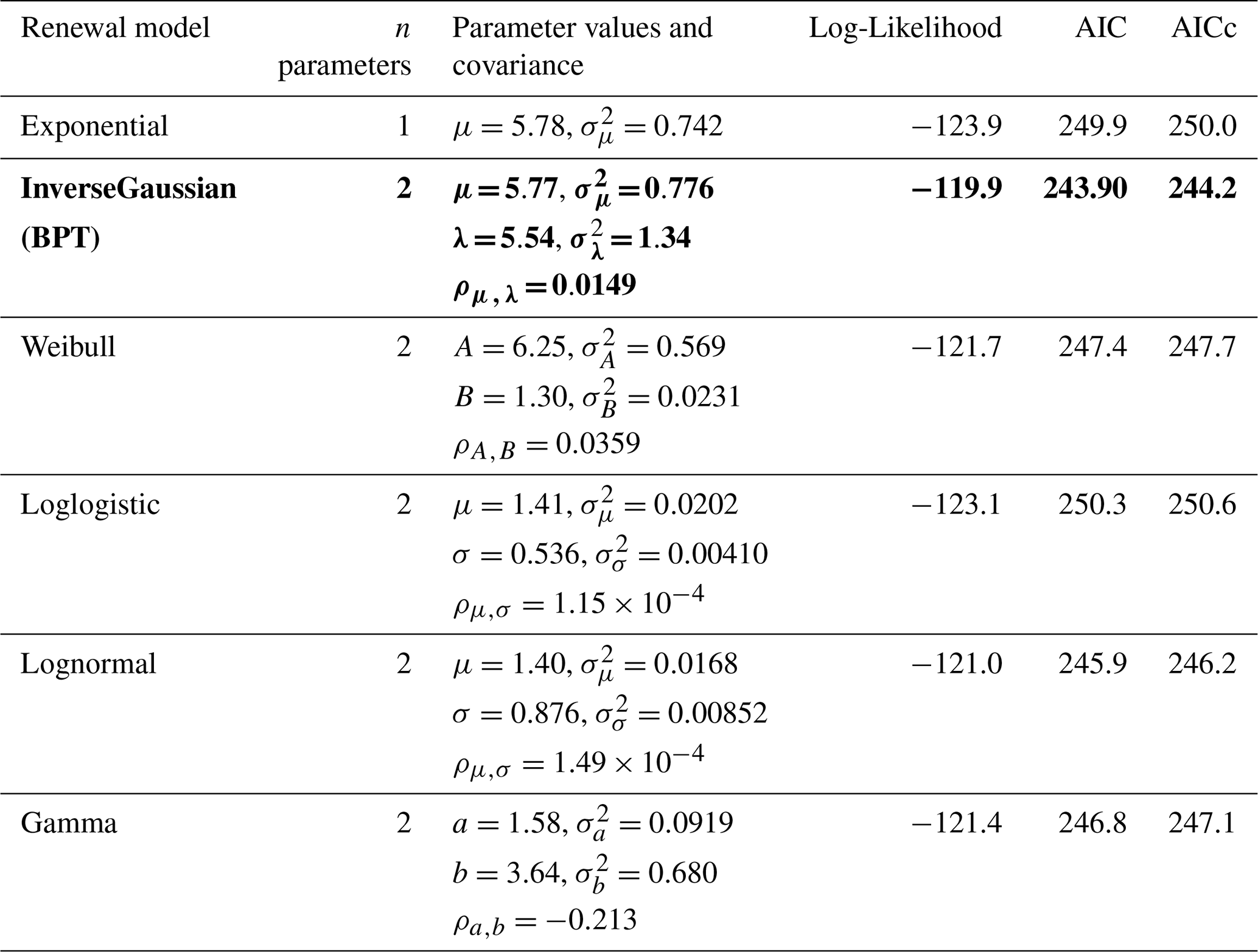
Among the best fitting renewal models, the one that is consistently preferred both by AIC and AICc is the Brownian Passage Time with parameters given in Table 2. The bootstrap KS1 test does not reject the null hypothesis of the real IETs being generated by that model (p-value = 0.154, while the 90 % confidence interval from bootstrapped samples is [0.069–0.218]). The fit of the best preferred model to the data is given in Fig. 1 where we compare its theoretical cumulative density function (red solid line) to the empirical cumulative density function of the real data (black solid line). In that figure we also show a whiskers plot of all the cumulative density functions of the 1000-sample models to account for the parameter uncertainty.

Figure 1 Comparison of the cumulative density function of the preferred model with best-fit parameters (light red solid line) to the empirical cumulative density function of the real IETs for flank eruptions (data since 1760 CE, dark red thick solid line), and the same for incremental distribution (thin blue and thick dark blue, respectively). The whiskers show the preferred model's variability (boxes: 25th–75th percentiles range; orange/blue lines show the range of all the models not considered outliers, and orange/blue dots show the models considered outliers, for the cumulative and incremental distributions respectively).

Figure 2 (a) Hazard function of the best fit preferred model for flank eruptions (Brownian Passage Time in thick solid green) and, for comparison, the corresponding hazard rate for a Poissonian process (Exponential distribution, black thin solid line); (b) probability of flank eruptions as a function of the exposure time, considering the current censoring time since last eruption in 2018, according to the preferred model (Brownian Passage Time in thick solid orange line) and 90 % confidence interval considering the uncertainty on the best model's parameters; (c) hazard functions for the Inter-Cluster (blue line, left axis) and Intra-Cluster (red line, right axis) for the IETs among summit paroxysms. The black thin line is for the Exponential model for Inter-Cluster IETs, for comparison (for Intra-Cluster, the rate is too high for the Poissonian occurrence to be suitable). (d) Expected number of summit paroxysms (solid thick purple line) and 90 % confidence interval, according to the best models describing the summit paroxysms IETs. The numbers of summit paroxysms over different ΔT are retrieved from the synthetic catalogs generated as explained in Sect. 4.2. Note the scale difference in x and y axes between the panels.

Table 3 First entry: Best evaluation (and 90 % confidence interval in brackets) of the probability of flank eruptions (considering the present censoring time since last flank eruption in 2018) for different exposure time windows (along columns). Second entry: best estimate (and 90 % confidence interval in brackets) of the expected number of summit paroxysms expected over the different time windows (along columns).

On the basis of the preferred model, we compute the hazard function for a flank eruption (Garcia-Aristizabal et al., 2012; Sandri et al., 2021), that is shown in Fig. 2a. The meaning of the Brownian Passage Time hazard function, depending on its parameters, is well explained in Fig. 2 of Matthews et al. (2002). Note that the term “hazard function” (also termed “hazard rate”) defines the instantaneous probability of a flank eruption as a function of the time elapsed since the last one, and should not be confused with the “hazard curve” (e.g., Tonini et al., 2015). Given the current censoring time (the time elapsed since the last flank eruption in 2018), in Table 3 we provide the probability of a flank eruption in the next 1, 3, 5, 10, 30 and 50 years, both based on the best-fitting parameters, and the 90 % confidence interval considering their uncertainty. We also show the probability of a flank eruption as a function of the exposure time window, according to the preferred model (Fig. 2b), with its 90 % confidence interval.

4.2 Summit paroxysms

Comparing the statistics in Table 1, we cannot reject the null hypothesis of stationarity for the catalog of observed summit paroxysms since 1986. A striking feature is the clear tendency toward clusterization (CV≫1). The best partition of the dataset into clusters of paroxysms, by means of k-means algorithm, identifies 12 clusters whose onset times are reported in Table 4. In Fig. 3 we show the cumulative number of summit paroxysms in time, with symbol colours that show the 12 different clusters identified.

Table 4 Start time of the 12 clusters identified with the best partitioning.

Figure 3 ECDF of the number of summit paroxysms observed at Etna between 1986 and 2022. The different colours highlight the different clusters identified by the k-means algorithm.

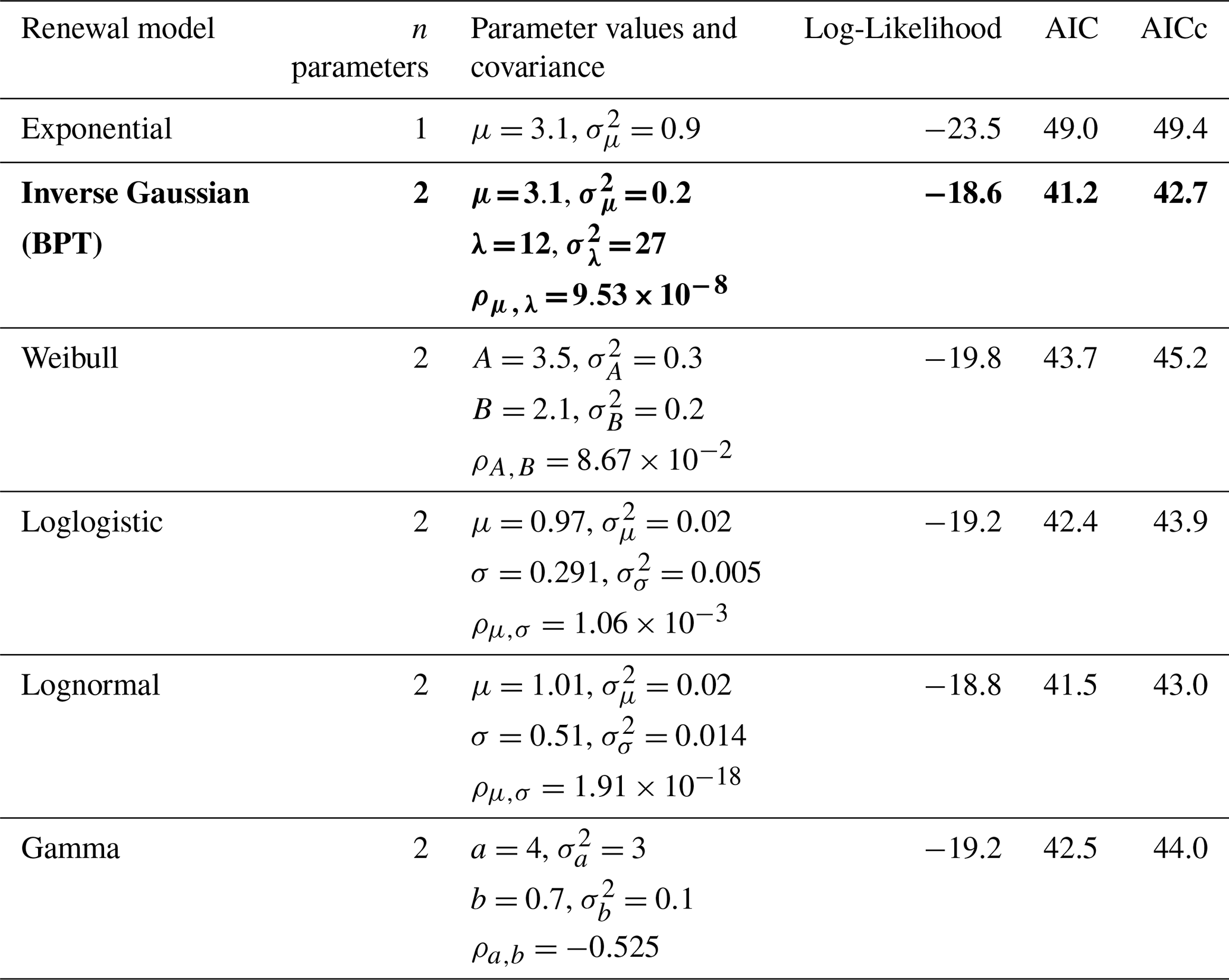
By applying the six renewal models considered to the Inter-Cluster onsets, the preferred model consistently identified both by AIC and AICc is again the Brownian Passage Time with parameters given in Table 5. In Fig. 2c we show in blue line the hazard rate for a new cluster to begin after the previous cluster's onset.

Table 5 Best fitting model parameters for the Inter-Cluster IETs, with variance (σ²) and, where there are more than 1 parameter, with covariance (ρ), for the 6 renewal models applied to the dataset of flank eruptions, and relative Log-Likelihood and value of Akaike Information Criterion (AIC) and its corrected version (AICc). In bold the preferred model according to the latter. All scale parameters are in unit of measure of years.

We then apply the six renewal models to the Intra-Cluster dataset, and again the preferred model by AIC and AICc is the Brownian Passage Time, with parameters given in Table 6. In Fig. 2c we show in red line the hazard rate for a new summit paroxysms to begin after the previous paroxysm's onset.

Table 6 Best fitting model parameters for the Intra-Cluster IETs, with variance (σ²) and, where there are more than 1 parameter, with covariance (ρ), for the 6 renewal models applied to the dataset of flank eruptions, and relative Log-Likelihood and value of Akaike Information Criterion (AIC). Here AICc coincide with AIC values, given the much larger number of IETs compared to the number of model parameters. In bold the preferred model according to AIC. All scale parameters are in unit of measure of years.

By combining the Brownian Passage Time models for Inter- and Intra-Cluster respectively, we generate 4000 synthetic catalogs spanning 35 years, which is the same duration of the real catalog of summit paroxysms (September 1986 to February 2022). To generate the kth synthetic catalog, we follow this procedure:

1. we generate 100 inter-cluster IETs (Δ_interT_i, i=1, …, 100) from their best Brownian Passage Time distribution, and we keep only the first N_k so that ${\sum }_{i=\mathrm{1}}^{N_k}{\mathrm{\Delta }}_{\mathrm{inter}}{T}_i\le \mathrm{35}$ years, and ${\sum }_{i=\mathrm{1}}^{N_k+\mathrm{1}}{\mathrm{\Delta }}_{\mathrm{inter}}{T}_i>\mathrm{35}$ years. These are the clusters' onset times.

2. for the jth cluster (j=1, …, N_k), we recursively generate n_jk Intra-Cluster IETs (Δ_intraT_i) from their best Brownian Passage Time distribution, until we generate an “extremely long” one. To define such an IET, we take a high percentile of the Intra-Cluster distribution, such as the 95th one. We assume that an extremely long IET means the cluster is over, and so we check that ${\sum }_{i=\mathrm{1}}^{n_{jk}}{\mathrm{\Delta }}_{\mathrm{intra}}{T}_i$ (where the set of n_jk IETs does not include the extremely long one) is shorter that the time between the onsets of the present (jth) cluster and of its subsequent one (the (j+1)th), otherwise the two clusters overlap. If the latter is the case, we discard the generated catalog and we start over again.

We repeat the last step procedure using different percentiles as threshold to define “extremely long” Intra-Cluster IETs, and keeping track of the number of times we need to discard the generated Intra-Cluster IETs and repeat the generation. Using percentiles up to 95th we do not discard a significant number of catalogs (less than 10 %), while going beyond the number of discarded catalogs increases dramatically (for example, about 50 % with 97.5th percentile). So we fix the threshold at the 95th percentile. In Fig. 2d we show the expected number of summit paroxysms (i.e., the mean among the 4000 synthetic catalogs) as a function of the exposure time window, along with its 90 % confidence interval.

To test the Inter- and Intra-Cluster temporal model, we test the capability of the synthetic catalogs in reproducing some key features of the real data of summit paroxysms.

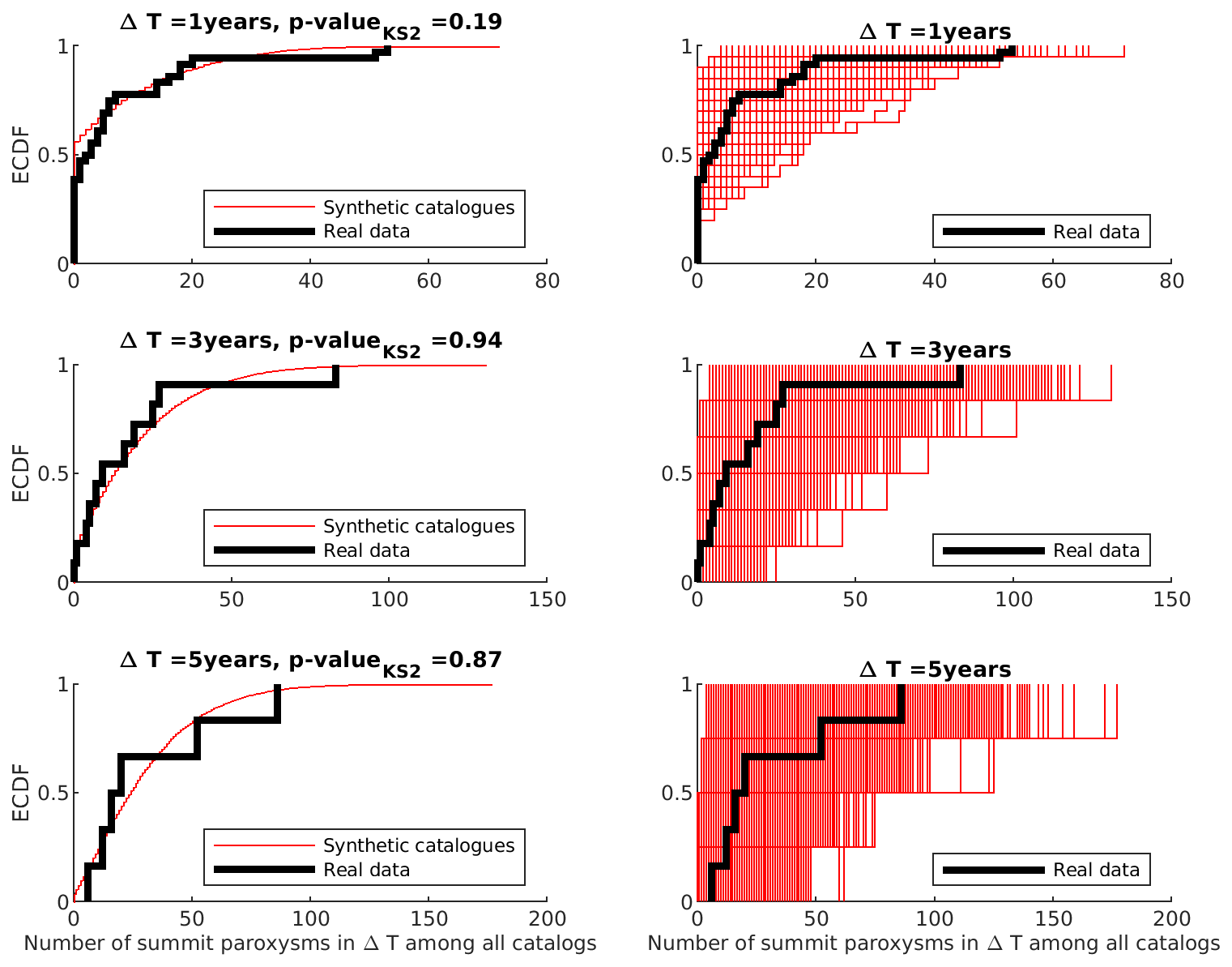
Figure 4 Left column: comparison of the empirical cumulative distribution function (ECDF) of the number of summit paroxysms observed over different time windows (1, 3 and 5 years, respectively upper, middle and bottom panels) in the real catalog (black thick line) and among the 4000 synthetic catalogs (red line), putting all the ΔT time windows from all catalogues together. The p-value of the KS2 test is shown in each panel's title line. Right column: comparison of the ECDF of the number of summit paroxysms observed over different time windows (1, 3 and 5 years, respectively upper, middle and bottom panels) in the real catalog (black thick line) with the 4000 individual ECDFs of the synthetic catalogues.

First, in Fig. 4 (left column plots) we compare the empirical cumulative distribution function (ECDF) of the number of summit paroxysms over time windows of 1, 3 and 5 years, in the real catalog and in the synthetic ones, putting all the synthetic time windows together. The simulated catalogs well reproduce the real data, and running a Kolmogorov-Smirnoff 2-sample test (KS2) on the samples of real and synthetic number of summit paroxysms over the three time windows considered does not allow to reject the null hypothesis of the two sets of data coming from the same parent distribution. We also compare, in Fig. 4 (right column plots), the real ECDF with the 4000 individual ones. Running individual KS2 tests between each individual ECDF and the real one leads to very few rejections (respectively, 17, 0 and 2 out of 4000 tests, at 1 % significance level, and 66, 2 and 20 at 5 % significance level).

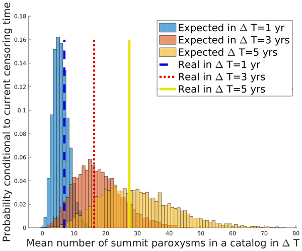
Secondly, we compare the mean number of summit paroxysms over the three time windows with the corresponding expected number in the simulated catalogs, as shown in Fig. 5. We see that the real mean number is very well captured by the synthetic data, especially for ΔT=3 and 5 years, whereas the annual mean number is slightly underestimated, although not significantly.

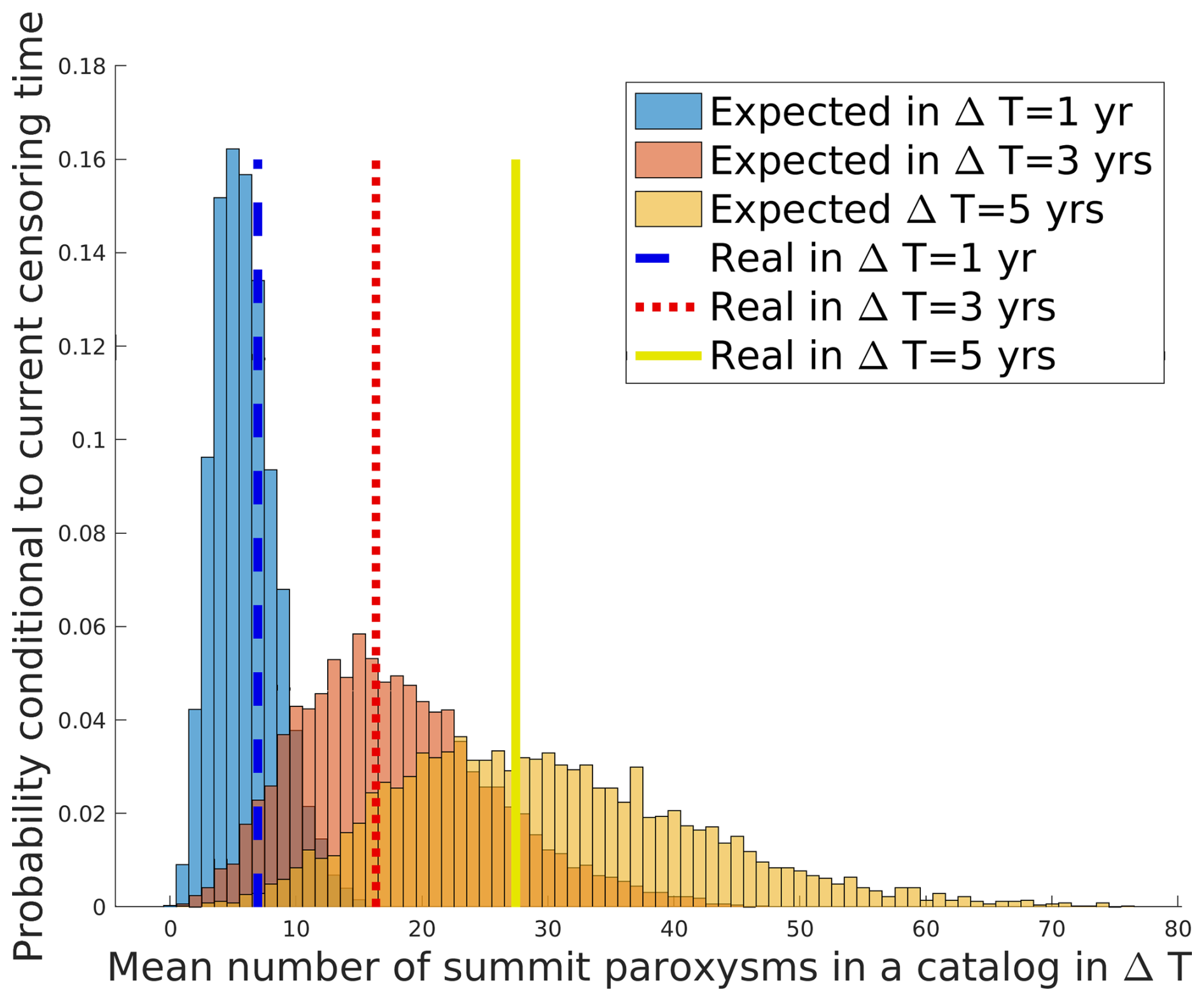
Figure 5 Histogram of the expected number of summit paroxysms over different time windows (1, 3 and 5 years, respectively in blue, orange and yellow) among the 4000 synthetic catalogs. The mean number in the real data is shown with dashed-blue, dotted-red and solid-yellow lines, respectively.

Last, in Fig. 6 we compare the distribution of the annual rate of summit paroxysms (Fig. 6a) and of clusters (Fig. 6b) in the synthetic catalogs with the real annual rates. We see that the real values are well captured by the synthetic catalogs, and the large p-values (null hypothesis is that the annual rate in the synthetic data is ≥ than the real one) do not allow discarding the model.

Figure 6 Histogram of the expected annual rates of summit paroxysms (a) and of clusters of summit paroxysms (b) across the 4000 synthetic catalogs. The red lines show the corresponding rate observed over the real data. In the title line we provide the p-value of the null hypothesis of a larger rate in the synthetic over the observed data.

5 Discussion

The models presented show that the occurrence of eruptions at Etna seems to be best described by a Brownian Passage Time model. This model has been previously used to model the occurrence of point processes such as seismic events (e.g., Matthews et al., 2002) or eruptions (e.g., Garcia-Aristizabal et al., 2012; Sandri et al., 2021). It is based on the so-called Brownian Relaxation Oscillator, in which a given state variable is subject to a constant loading with superimposed Brownian perturbations. An event occurs (i.e., the point process has a realization) when the state variable reaches a threshold. When this occurs, the state variable relaxes to the background value, and a new “stochastic” cycle begins. This leads to a stochastic load-state process. The load-state process is the Brownian Relaxation Oscillator, whose IETs are described by the Brownian Passage Time distribution (also termed Inverse Gaussian or Wald distribution in the literature). We remand the reader to Fig. 2 in Matthews et al. (2002) for a visual explanation of the Brownian Relaxation Oscillator. The state variable of this model can be linked to the tectonic loading for earthquake occurrence, or to the pressure in the magma storage system under a volcano (Sandri et al., 2021). The main feature of this type of renewal model is that, depending on the combination of the values of the 2 model parameters, the model is able to describe from a quasi-periodic occurrence up to a non-homogeneous Poisson process. As shown in Fig. 2, its hazard function increases in time after an event (with very different characteristic timescale, depending on the model parameters values) until a plateau is reached, which implies then a Poissonian occurrence (for comparison, in Fig. 2a and c we also provide the Poisson hazard function for the flank and inter-cluster IETs).

For flank eruptions, assuming stationarity to retain the complete part of the catalogue, we consider as complete the eruptive record since 1760 CE. Under this assumption, here we cut out from the catalogue the unusually long IET that follows the largest eruption occurred in 1669 CE. We acknowledge that this long IET might be real and may reflect the “generalized” (i.e., not linear) time-predictable behaviour suggested by e.g. Marzocchi and Zaccarelli (2006) and Passarelli et al. (2010), although those studies used a different and less revised catalogue. Here, we base our study on the most recent available catalogue for flank eruptions at Etna (Proietti and Branca, 2024) and the unusually long IET following that large eruption breaks the stationarity assumption. Thus we removed it, suspecting a possible incompleteness in the aftermath of such a large eruption which destroyed Catania layout and may have disrupted the recording of Etna eruptions. In any case, since 1760 CE, based on the value of the CV, no significant clustering is observed so we model the occurrence of these events simply by the preferred renewal model (Brownian Passage Time). The bootstrap version of the KS1 test for the goodness of fit does not reject the model. We compare the performance of the preferred model to the “reference” Poissonian occurrence over the IET data among flank eruptions, by computing the individual probability gain for each event (as we do not know the exact day and month of each eruption, we consider the probability over the year of occurrence of each eruption), and the overall gain (Kagan and Knopoff, 1987; Passarelli et al., 2010). We see in Fig. 7 that the preferred model outperforms the reference Poissonian occurrence when the IET is “not too short” (approximately larger than 1 year) and “not too long” (i.e., within 6 years since the previous event). Over the whole dataset, the probability gain of the Brownian Passage Time with respect to Poissonian occurrence is positive (value is 0.073).

Figure 7 Individual probability gain of the preferred model for flank eruptions (Brownian Passage Time) with respect to the Poissonian occurrence, by event (IET on x-axis). In green the events for which the Brownian Passage Time outperforms the reference model, in red otherwise. The overall probability gain is 0.073.

By means of the preferred model identified and based on BPT, we compute the probability of flank eruption over different time windows (see Fig. 2b and Table 1). Considering the uncertainty on the model parameters, we compute uncertainty intervals on this best estimate probability. Even considering the lower limit of this interval, we see that flank eruptions have a probability above 95 % over a window of 30 years, considering the current censoring time.

Summit paroxysms at Etna clearly show a clustered behaviour, so we model separately the inter-event between cluster onsets and the IETs of events within clusters. Again both preferred models are the Brownian Passage Time, with different parameters' values. The testing of this model is not as straightfoward as in the case of flank eruptions. To perform the test, we use the preferred models to generate synthetic catalogs and then we test how they capture some basic features of the real dataset of summit paroxysms. Synthetically-generated catalogs well capture the real observations for summit paroxysms in terms of (i) distribution of the number of events over three time windows (1, 3 ad 5 years, Fig. 4) and their means (Fig. 5), and (ii) annual rates of events and of clusters (Fig. 6). So we judge the two Brownian Passage Time models good in describing the occurrence of Etna summit paroxysms in clusters, and we compute their expected number over 1, 3 and 5 years (Table 3). The best guess in 1 year is 6 paroxysms, with a 90 % confidence interval from 0 to 28.

In order to present how the latter model for summit paroxysms can be used in practical applications, we provide an illustrative example. To this end, we use the synthetic catalogs to simulate the temporal component of a Probabilistic Volcanic Hazard Assessment (PVHA) for the tephra fallout caused by Etna summit paroxysms. Since we cannot simulate wind field from the future, we pre-run 3500 simulations of tephra fallout from Etna summit craters with TEPHRA2 model (Bonadonna et al., 2005) by sampling random dates (day, month, year, hour and minute) over the period 2007–2019, thus covering 13 years, for which the wind field is available from INGV-OE daily weather data (Scollo et al., 2009). Each TEPHRA2 run had associated a set of Eruption Source Parameters (Mass Eruption Rate and Duration of fallout phase) that was sampled from Empirical Cumulative Distribution Function of the real observations (for the events for which they are available, Andronico et al., 2021; Mereu et al., 2023; Scollo et al., 2025). The computational domain of TEPHRA2 simulations covers 14.1960 to 16.148° E and 37.041 to 38.578° N, at 500 m resolution.

Figure 8 Example to show how the preferred model is used in practice into a hazard assessment workflow. Panel (a) shows an example of synthetic catalog generated from the preferred model for summit paroxysms (blue lines mark the beginning of synthetic clusters, 9 in the example shown, and red lines mark the occurrence of events within clusters). Panel (b) shows in green lines all the simulated tephra dispersals (3500 simulations covering random times between 1 January 2007 and 31 December 2019). In blue and red lines we mark the tephra dispersal associated to each synthetic event in panel (a) (again blue and red mark cluster onset and Intra-Cluster events), in which the seasonal correspondence is respected, but the year is shifted as explained in the text. The same numbering of clusters as in panel (a) is given. In panel (c) we show the distribution of the time difference between the month, day and hour of the tephra simulation and of the synthetic event.

Figure 9 Example of the obtained hazard results for tephra ground load from paroxysmal activity. Panel (a) shows the Hazard Curve for the accumulation of tephra load (from summit paroxysms) at the ground in 1 year at Milo, located in the South East side of Etna volcano (thick solid line is the mean hazard curve, whereas thin solid lines provide the 90 % confidence band). Panels (b) and (c) show respectively the probability maps of accumulating at least 5 cm in a cluster of summit paroxysms, and at least 1 cm in 1 year (still from paroxysms).

We then took 1000 synthetic catalogs of summit paroxysms from the temporal model analysis, and cut them over the period 2024–2048, thus covering 25 years in the future (at the time of the analysis, made in 2023–2024). To each synthetic paroxysm (with a date from 2024 to 2048) we associated the deposit of the pre-simulated eruption that was closest in time among the set of pre-run simulations, after subtracting 17 or 30 from the year of the synthetic event respectively form synthetic years from 2024 to 2036 and 2037 to 2048. In this way we preserve seasonality and, for clusters of synthetic events occurring close in time, we preserve the natural persistence or evolution of the wind field in time, as in reality. An example of this procedure for a specific synthetic catalog is provided in Fig. 8. The deposits corresponding to the synthetic events were then combined to achieve, on the grid points of TEPHRA2 computational domain, hazard curves of the accumulated tephra at the ground during a paroxysm, during a cluster, and in time windows of 1, 3 and 5 years (for example Fig. 9a). By cutting the hazard curves at selected tephra load or exceedance probability thresholds, we obtain respectively probability and hazard maps (Tonini et al., 2015, see for example Fig. 9b and c).

6 Conclusions

In this study we have modelled the occurrence in time of relevant eruptive events at Etna volcano, the most active volcano in Europe located North of the metropolitan area of Catania (Sicily, Italy). We have separately accounted for flank eruptions and for summit paroxysms. The former events are more rare, but are capable of producing lava flows that can reach inhabited areas, and of generating tephra emissions over periods of months (as in 2002–2003; Andronico et al., 2008). The latter type of activity is very frequent (around 260 events have occurred in the period of time analyzed here, 1986–2022) and generates short-lived plumes (up to few hours long) that have reached up to 14–15 km above the summit of the volcano, at 3360 m a.s.l. approximately. These plumes can threaten local mobility by accumulating tephra on the roads, as well as air traffic in the area. Moreover, occurring in clusters during which these events are typically separated by few days up to few weeks, they can represent a problem in terms of clean up operations (e.g., Mereu et al., 2025).

By considering the most recent catalog of flank eruptions at Etna (Proietti and Branca, 2024) and assuming stationarity, we consider as complete the data since 1760. The flank eruptions recorded from that date do not show any tendency to clustering. Their inter-event times are best modelled by a Brownian Passage Time distribution. The preferred model, with its maximum-likelihood parameters and their uncertainty, well capture the cumulative distribution of the observed inter-flank-eruptions times.

For summit paroxysms, due to their evident clusterization, we first apply a k-means algorithm to the dataset of summit paroxysms (see Supplement), to objectively find the best partitioning into k clusters. We find that k=12 yields to the best partition, according to the mean silhouette coefficient. We then model separately the Inter-Cluster onset times and the inter-event times between successive paroxysms belonging to clusters. We find that both subsets of data are best described again by a Brownian Passage Time distribution, with very different parameter values. In order to judge the capability of these models in reproducing the basic features of the real inter-paroxysms times, we use the two preferred models to generate synthetic catalogs, that we then analyze. We find that the synthetic catalogs overall capture the real observed and mean number of paroxysms over different time windows (1, 3 and 5 years), and annual rate of clusters and of paroxysms. Finally, we have given an example on how to use in practice these two preferred model to introduce the temporal variability in hazard assessment. In particular, we have provided an illustrative example on how the synthetic catalogs can be coupled to a set of pre-run tephra dispersion simulations in order to quantify the ground load hazard for a paroxysm, for a cluster, or over a time window of 1, 3 and 5 years.