Assessing the spatial correlation of potential compound flooding in the United States

When coastal and river floods occur concurrently or in close succession, they can cause a compound flood with significantly higher impacts. While our understanding of compound flooding has improved over the past decade, no studies to date have assessed the spatial correlation of compound flooding. To address this gap, we develop a framework that captures dependence between coastal total water level and river discharge across a set of locations along the US coastline. Using 41 years of observed data from 41 station combinations, we stochastically model 10 000 years of spatially-joint events of extreme sea level and river discharge based on their dependence structure and cooccurrence rate. We define potential compound flooding as events in which both drivers exceed their respective 99th percentile thresholds. Results based on our simulated large event set show that the US West coast shows high spatial correlation of potential compound flooding. Among all three coasts, the West coast has the highest frequency of widespread potential compound flooding, with around 50 % of compound events arising at multiple locations simultaneously. We identify two clusters with mutually high joint occurrence rates of simultaneous compound events on this coast, namely (1) Charleston – Crescent City – North Spit, and (2) Santa Monica – Los Angeles – La Jolla. Widespread compound events are less frequent on the East coast where approximately 30 % of potential compound flooding may affect multiple locations. Moderate spatial dependence is observed in the central region and weaker spatial dependence for the remaining locations on this coast. In contrast, the Gulf coast shows the weakest spatial correlation, where over 82 % of compound events only affect single locations. Our findings highlight the importance of accounting for spatial dependence in compound flood assessments. Our large set of stochastic spatially-joint events can be used as boundary conditions for the hydrologic-hydraulic models to simulate the surface inundation and further assess risks of compound flooding in low-lying coastal and estuarine areas.

1 Introduction

In the contiguous United States, coastal counties are home to nearly 129 million people (NOAA, 2020) and often serve as important economic centres (McGranahan et al., 2007). In these low-lying, densely populated areas, flooding can cause widespread adverse socioeconomic and environmental impacts, with an estimated annual damage of more than USD 180 billion (JEC, 2024). Despite continued investments in flood adaptation and management, recent flood events, such as Hurricanes Milton, Helene, and Ida, have demonstrated the ever-present threat of serious flood impacts in coastal regions. Flood water levels in these areas can be influenced by both coastal drivers (e.g. high tides, wave action, and storm surges) and riverine drivers (i.e. heavy precipitation and high river discharges). When multiple drivers coincide or occur in close succession, they can result in a compound flood event that intensifies the overall flood hazard and causes significantly higher impacts than when they occur in isolation. Moreover, these flood drivers are projected to co-occur more frequently in the US due to climate change factors including sea level rise (Ghanbari et al., 2021), potential changes in tropical cyclone climatology (Gori and Lin, 2022), and projected shifts in future river flow regimes (Moftakhari et al., 2017). Together with projected shoreline deformation (Woodruff et al., 2013) and socio-economic growth (Hallegatte et al., 2013), these changes are expected to escalate compound flood risk in most US coastal areas in the future.

Compound flooding in coastal and estuarine regions can be driven by several mechanisms (Jane et al., 2025). First, both storm surge and rainfall (or river discharge) are extreme to cause flooding and their interaction can increase the flood extent and depth. Second, storm surge and rainfall are moderate and do not cause flooding individually but their interaction may initiate flooding. Third, extreme sea levels alone can cause flooding and additional rainfalls can further intensify the flooding. Fourth, high water levels (not necessarily being extreme) can (1) create backwater effects and block free river flows to the sea (Ghanbari et al., 2021), and (2) impede efficient drainage of heavy rainfall (Wahl et al., 2015), thereby prolonging or increasing flooding. Synoptic weather patterns, both tropical cyclones (TCs) and extra tropical cyclones (ETCs), are the main drivers of these compound flooding mechanisms worldwide (Lai et al., 2021). While TCs tend to cause extreme flooding, ETCs are found to be responsible for more frequent and moderate events (Booth et al., 2016; Gori and Lin, 2022). Besides synoptic weather patterns, coastal and river floods can also co-occur by coincidence (Couasnon et al., 2020); however, such incidents are considered statistically independent according to probability theory (Martius et al., 2016). Traditional flood risk assessments do not consider these interactions between flood drivers and may therefore underestimate the overall flood hazard and associated risk (Wahl et al., 2015; Ward et al., 2018). Having more accurate assessments of compound flood risk could help in the development of effective adaptation measures to reduce current and future risks.

A key step in compound flood risk assessment is accurately quantifying the dependence and joint probabilities among flood drivers. These quantifications can provide essential boundary conditions for flood hazard and risk assessments (Eilander et al., 2023; Moftakhari et al., 2019), and are important for designing flood protection measures in regions prone to compound flooding (Salvadori et al., 2016; Ward et al., 2018). In recent years, there has been a growing body of research assessing the dependence between coastal and riverine flood drivers over a range of spatial scales. Most of these studies (e.g. Bevacqua et al., 2017; Couasnon et al., 2018; Rueda et al., 2016) are focused on specific locations due to the complexity of the applied multivariate statistical models. At larger spatial scales (regional to global), dependence assessments are often limited to bivariate cases involving two flood drivers (e.g. Bevacqua et al., 2019; Couasnon et al., 2020; Ward et al., 2018), while a few studies (e.g. Camus et al., 2021; Nasr et al., 2021) considered three or four drivers. For the entire US coastline, compound flooding potential has been evaluated by several studies in terms of statistical dependence between storm surge and rainfall (Wahl et al., 2015), joint probabilities of coastal water level and river discharge under sea level rise scenarios (Ghanbari et al., 2021; Moftakhari et al., 2017), and seasonal patterns in the dependence structure among storm surge, wave, river discharge, and rainfall-runoff (Nasr et al., 2021).

While these studies have improved our understanding of compound flooding, no studies to date have looked into the spatial correlation of compound flooding between locations. Significant spatial dependence has been identified for both coastal (Enríquez et al., 2020; Li et al., 2023) and riverine flooding (Metin et al., 2020; Quinn et al., 2019) in the United States. Moreover, the storm events TCs and ETCs that may drive compound flooding can have a large spatial footprint. Therefore it is likely that compound flooding may potentially arise across multiple locations. A recent example of widespread compound flooding is Hurricane Harvey in 2017. It caused record-breaking rainfall, river discharge, and run-off, combined with a moderate but long-lasting storm surge, resulting in disastrous flooding in Houston (Valle-Levinson et al., 2020). Simultaneously, other regions including Galveston Bay, Rockport, and Richmond also saw flooding.

Therefore, the overall aim of the paper is to assess the spatial correlation of potential compound flooding from extreme sea level and river discharge along the US coastline. Potential compound flooding is defined as events during which both extreme sea level and river discharge exceed the corresponding 99th threshold. To this end, three objectives are addressed. First, we estimate the statistical dependence between extreme sea level and river discharge across different locations, while accounting for relevant time lags. This includes a multivariate statistical sampling for identifying observed spatially joint events with potential compound flooding (i.e. cooccurring events across different locations), and applying a multivariate conditional statistical model to these events to estimate the dependence structure both spatially and between extreme sea level and river discharge. The second objective is to develop an equivalent of 10 000 years of stochastic spatially joint events based on the estimated dependence, which can be used as boundary conditions for physical flood inundation models. Based on the stochastic events, the third objective is then to assess the spatial correlation of compound flood potential by looking into the co-occurrence of extreme sea level and river discharge at different locations.

2 Data and Methodology

To investigate the spatial correlation of potential compound flooding events around the US coasts, we assess dependence between coastal and riverine flooding drivers, specifically extreme sea levels and river discharges in this study. The dependence structure is also assessed between these drivers across different locations. This study involves the following five steps, which are described in the subsections:

• 1.

  Selecting datasets and station combinations of tidal gauges and river discharge stations along the US coastline;

• 2.

  Infilling missing values of sea level and river discharge time series;

• 3.

  Identifying joint extreme events of sea levels and river discharges at different locations;

• 4.

  Estimating the dependence structure from the identified events and generating 10 000 years of stochastic spatially joint events using a multivariate conditional statistical model;

• 5.

  Assessing the co-occurrence of different extreme events at different locations from the generated stochastic events.

2.1 Datasets and selection of station combinations along the coastal US

For sea levels, we use the observed hourly total water levels for the period 1980–2020 from the Global Extreme Sea-level Analysis Version 3 database (GESLA-3) (Haigh et al., 2023). These coastal water levels consist of mean sea levels, astronomical tides, and non-tidal residuals (i.e. storm surges). For the river component, we use river discharge because it represents near-term runoff from a storm event that contributes to the riverine water levels (Bevacqua et al., 2020). Therefore, daily mean discharge observations between 1980 and 2020 are extracted from the United States Geological Survey (USGS) network (https://waterdata.usgs.gov/nwis/rt, 5 March 2025).

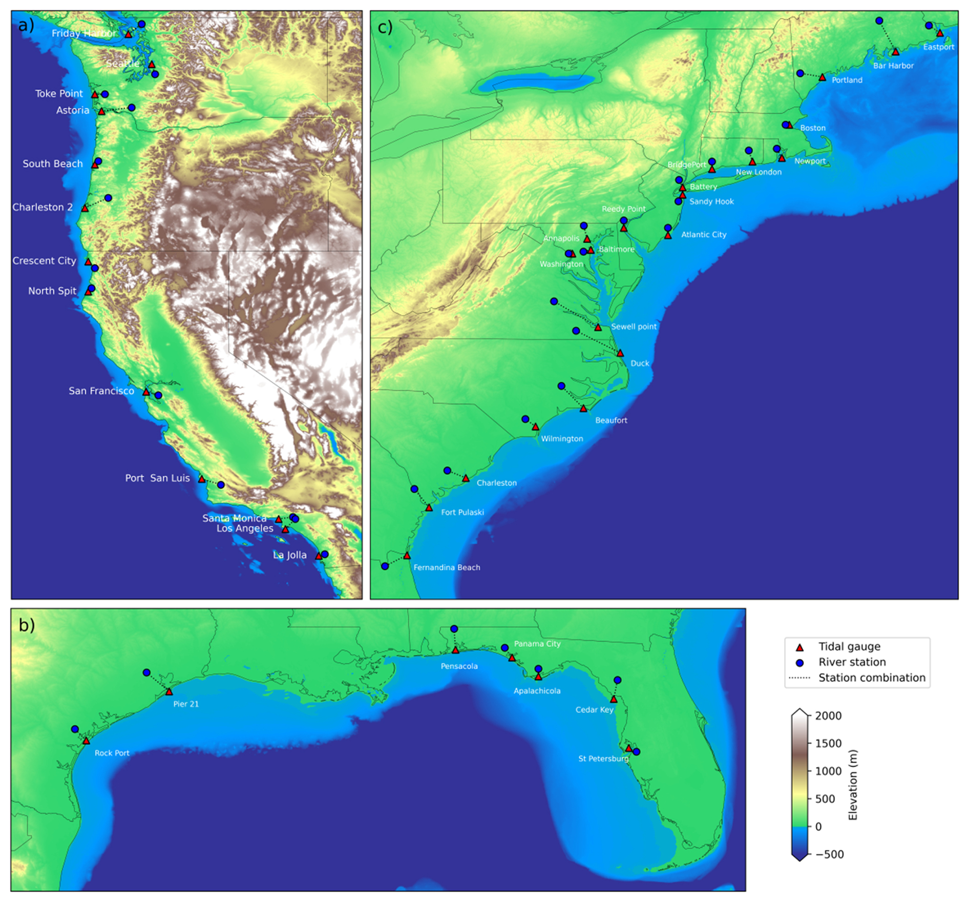
Figure 1 The location of station combinations on the US (a) West, (b) Gulf, and (c) East coasts. The red triangles and blue circles represent the selected NOAA tidal gauges and USGS river discharge stations in this study.

For a spatially extensive coverage of coastal locations, we select 41 GESLA-3 tidal gauges by combining stations used in previous studies (Feng et al., 2023; Ghanbari et al., 2021; Nasr et al., 2021; Wahl et al., 2015). These 41 tidal gauges are then paired with nearby USGS river stations, following the selection criteria based on Nasr et al. (2021) and Ward et al. (2018): (1) minimum data completeness of 80 % during 1980–2020 in the daily mean discharge time series; (2) minimum upstream catchment area of 1000 km²; (3) maximum Euclidean distance of 500 km from the tidal gauge; and (4) maximum distance of 55 km (0.5°) between the river outlet and the tidal gauge. For some tidal gauges, several USGS river discharge stations satisfy these rules. In these cases, we select the ones with the most complete data records preferably in the downstream area. The full selection procedure results in 13, 7, and 21 station combinations for the West coast, Gulf of Mexico, and East coast, respectively. Figure 1 shows the locations of these station combinations and further information can be found in Table S1 in the Supplement.

When characterising dependence, standard extreme-value theory statistical models require that the input datasets consist of independent and identically distributed (i.i.d) variables. To satisfy this assumption, we first detrend the hourly total water level records by removing the long-term mean sea level signal. This is achieved by subtracting the annual mean sea level using a moving window, thereby filtering out the inter-annual to multi-decadal sea level variability (Valle-Levinson et al., 2017). River discharges do not show such long-term variations, and so no detrending is applied to the daily mean records. To prepare for the independence processing and maintain temporal consistency between total water level and river discharge, we further aggregate the hourly sea levels into daily maxima. The independence is then ensured by applying a 5 d de-clustering window (Camus et al., 2021; Maduwantha et al., 2024) with the maximum value centred in each window.

2.2 Infilling missing values of sea levels and river discharges

Gauge observation records often suffer from data gaps and may preclude a robust statistical dependence analysis between flood drivers. Compound flood studies (e.g. Nasr et al., 2021; Wahl et al., 2015; Ward et al., 2018) that only estimate the dependence structure between pairs of stations are less affected by these data gaps and do not attempt to infill missing observations. As this study also investigates dependence across locations, constraining the analysis to common time periods without missing data would likely result in very few overlapping events. We calculate the length of the 41 year observational data with removed gaps. The data length sharply decreases from 41 years to 11.4 years for the West coast and to 3.2 years for the combined Gulf and East coasts when only gap-free records are used, see Table S3. Using such short overlapping data would be insufficient to robustly estimate the dependence structure.

To address this issue, other studies (e.g. Jane et al., 2020; Quinn et al., 2019) infill data gaps or missing values using simultaneous values from nearby stations. This prepares complete time series for dependence estimation, but this approach may introduce artificial signals such as increased correlation between locations. To preserve sufficient data coverage across locations, we infill missing values in the time series at those 41 combinations of tidal gauges and river stations. Across all locations, the averaged infilling percentage is 1.73 % (i.e. equivalent to 0.71 years) for the 41 observation years between 1980 and 2020, see Table S3. For daily maximum total water levels, each of these 41 tidal gauges has missing values in daily maximum sea levels, with 33 gauges missing less than 1 year of data. Two gauges, Santa Monica and Bar Harbor, show the lowest data completeness, with 3.2 and 3.6 years of missing values, respectively. For daily river discharges, 10 stations contain missing values where six stations have gaps of less than one month, two stations have missing data up to two years, and one station (Cowlitz River) is missing 7.5 years of data.

To infill missing total water levels, long data gaps are first imputed using linear regression based on simultaneous water levels from nearby tide gauges located within 50 km. We start the infilling process with the nearest available gauge and retain only the values estimated from regressions with a coefficient of determination (R²) greater than 0.5. For some tide gauges where no gauges or only a few ones without available data exist within the 50 km radius, we increase the search distance to 150 km. The remaining non-consecutive gaps are subsequently filled using linear interpolation.

Missing daily mean river discharges are first translated from the corresponding gage height observations using rating curves. These curves describe the empirical linear correlation between gage height and mean river discharge for individual stations and are available from the USGS website (https://waterwatch.usgs.gov/index.php?id=ww_toolkit, last access: 15 March 2025). The remaining missing values are then infilled using linear regression with daily mean discharges from the nearest upstream river station. If there are more than one upstream river inlets, multi-linear regression is applied to estimate the missing discharges based on simultaneous data records at all upstream stations. Lastly, any remaining discrete missing discharges are calculated through linear interpolation. As an example, Fig. S1 in the Supplement shows the data infilling result at the tidal gauge Santa Monica (3.2 years of missing data) and the river station Cowlitz River (7.5 years of missing data), as well as the methods adopted to impute specific missing values.

2.3 Identifying spatially joint extreme events of sea levels and river discharges

Storm events can impact a large stretch of coastline (Enríquez et al., 2020; Li et al., 2023) and may cause compound flooding at multiple locations. However, individual storms are not likely to affect all parts of the US coastline. To account for this trade-off and spatial dependence, we develop datasets of spatially joint extreme events of total water levels and river discharges for two coastal regions: (1) the West Coast, and (2) the combined Gulf of Mexico and East Coast. We group the Gulf and East coasts together because hurricanes can make landfalls in close succession across these two regions. Prime examples of such events are Hurricanes Helene (2024), Ian (2022) and Katrina (2005).

For each region, we first define joint extreme events that may potentially cause compound flooding at individual locations/station combinations. This analysis involves a two-sided conditional sampling where bivariate events are selected conditioned on one of the two drivers (i.e. total water levels and river discharges) being extreme (Jane et al., 2020). Due to the relatively short data records used in this study, we use the peak-over-threshold (POT) approach for this process as POT generally samples more extreme events compared to the annual maxima approach (Camus et al., 2021). However, the POT approach introduces subjectivity in threshold selection: the threshold should be high enough to drive a good fit of marginal distributions, yet low enough to ensure sufficient samples for robust parameter estimation of these distributions. To reduce this subjectivity, we apply the automated threshold estimation approach of Solari et al. (2017) to total water level and river discharge time series to sample joint extreme events at each station combination. We account for potential time lags between the peak water level and river discharge by allowing a ± 3 d lag. When conditioned on total water levels, a peak water level is paired with the maximum river discharge occurring within a 7 d window centred on that water level; the same procedure is used for cases conditioned on river discharges. When identifying these extreme events, we follow previous studies (e.g. Couasnon et al., 2020; Ghanbari et al., 2021; Jane et al., 2020; Wahl et al., 2015; Ward et al., 2018) and assume that all events arise from a single population. This simplifying assumption therefore does not account for the mixed-population effects caused by events generated by different storms (e.g. TCs and ETCs) and hydrological processes (e.g. snowmelt and convective rainfall).

These bivariate extreme events at individual locations are then grouped into a large dataset for each study region. To do this, we consider a set of m locations (i.e. 13 and 28 station combinations for the West and the combined Gulf and East coasts). At location i, we use a bivariate vector $X_i=({\mathrm{TWL}}_i,Q_i)$ where TWL_i and Q_i represent time series of paired total water level and river discharge. The set of these components for each study region is then defined as $\mathbf{X}=\mathit{\{}{X}_i,i\in \mathit{\{}\mathrm{1},\mathrm{\dots },m\mathit{\left\}}\mathit{\right\}}$.

We further transform X onto a common marginal scale. Laplace margins are adopted in this study because they have been shown to outperform other common marginals such as Gumbel distributions in the subsequent dependence modelling framework (Keef et al., 2013). For the set X, the transformation is achieved by:

$$\begin{array}{}\text{(1)}& Y_i=\left\{\begin{array}{l}\text{log}\mathit{\left\{}\mathrm{2}{F}_i\right(X_i\left)\mathit{\right\}},X_i<F_i^{-\mathrm{1}}\left(\mathrm{0.5}\right)\\ -\text{log}\mathit{\left\{}\mathrm{2}\right[\mathrm{1}-F_i\left(X_i\right)\left]\mathit{\right\}},X_i\ge F_i^{-\mathrm{1}}\left(\mathrm{0.5}\right)\end{array}\right.\end{array}$$

where F_i is the marginal distribution of X_i. The marginal distribution F_i is semi-parametric and estimated independently per component at individual locations. For each water level or river discharge component, a generalised Pareto distribution (GPD) is fitted to detrended and de-clustered peak values above a specified threshold while an empirical distribution is used for those below the threshold. We use the previously identified thresholds for this process and the underlined GPD fitting is performed through penalised likelihood estimation using a Gaussian prior. To assess the sensitivity of the transformation results to different marginal distributions; we also test Gumbel marginals and find that the results are insensitive to this choice.

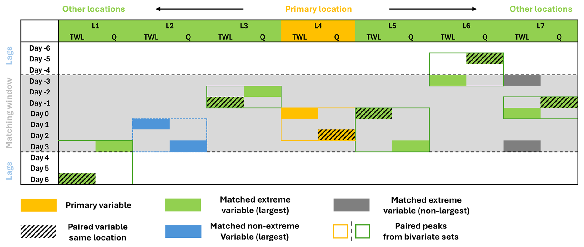
Figure 2 Schematic of the construction of one spatially joint events across the 7 locations of an exemplary coastal region. SWL refers to total water level while Q refers to river discharge. The orange cell indicates the primary variable with the largest marginal value at the primary location. For other locations, matched extreme variables are marked in green where the maximum of either TWL or Q within the matching window is selected. Dark grey cells are the available extremes within the window but they are not the largest. Hatched cells are the paired peaks to the matched variable from the bivariate events identified for individual locations. Blue cells indicate the matched non-extreme variables; they are not from paired bivariate peaks and are marked by a blue dashed box.

From each transformed set ${\mathbf{Y}}_{\text{trans}}=\mathit{\{}{Y}_i,i\in \mathit{\{}\mathrm{1},\mathrm{\dots },m\mathit{\left\}}\mathit{\right\}}$, we identify spatially joint events across the entire coastal region, see Fig. 2 for an example of constructing one such event for a region with 7 locations. To do this, we first identify the primary variable with the largest marginal value (e.g. the water level at location 4, marked in orange) among all variables from the entire dataset, and retrieve the occurrence date and location. At this primary location, we then obtain the corresponding value for the other variable (e.g. the river discharge in the hatched orange cell) from the sampled bivariate events. For instance, if the largest extreme water level event occurs at a coastal station, we obtain the corresponding river discharge value at the paired river station from the bivariate event set developed for individual locations.

Next, we match this primary event at the primary location to potential bivariate events at all other locations. Since peaks at different locations do not necessarily occur simultaneously, we apply a time window of 7 d (± 3 d around the peak for the primary variable) in the matching process. In other words, we assess whether a compound event occurs at another location within this time window. This process may result in multiple bivariate events identified for a single location (e.g. the three extreme water level identified at location 7); in these cases, we retain the event with the largest marginal peak (e.g. the event marked by a green square at location 7). If no event is found for a particular location (e.g. the case for location 2), we instead select the maximum total water level or river discharge (e.g. the blue cells at location 2) within the 7 d window. This process samples one spatially joint event for the entire coastal region centred around the peak of the primary variable. Once this event is identified, we remove all peaks across all variables and locations that fall within the associated event window (ranging from 7 to 13 d, depending on the timing of the matched peaks). We then repeat the process with the updated event set, identifying the next largest remaining marginal value to define the corresponding spatially joint event. This iterative sampling continues until no peaks can be found in the event set.

This approach generates a separate dataset Y of spatially joint events of total water level and river discharge from the large transformed dataset Y_trans with time series of paired peaks for the two study regions in this study. Each sampled event represents a peak bivariate event at a single location (the primary station combination) matched appropriately with potential peak bivariate events at all other locations. The validity of these spatially joint events is ensured by performing several measures (see Sect. S1 in the Supplement), and results of these measures can be found in Figs. S2 and S3.

2.4 Estimating the statistical dependence structure and generating a 10 000 year of spatially joint events of total water level and river discharge

2.4.1 Dependence calculation

To assess the dependence structure between a set of variables, two main classes of statistical models have been typically used: (1) copulas, and (2) the multivariate conditional model of Heffernan and Tawn (2004). Standard copulas are used to describe the bivariate dependence while pair-copula construction (e.g. vine copula) is developed to assess higher-dimensional dependence. Although the copula approach has been widely used in compound flooding analyses, standard copulas impose one type of extremal dependence in the joint tails between variables (Heffernan, 2001). Therefore, a priori selection of the best-fit copula is often performed for paired variables of interest (e.g. Jane et al., 2020; Wahl et al., 2015). In contrast, the multivariate conditional model captures the dependence structure between a set of variables by estimating the conditional distribution for the remaining variables given that a primary variable exceeds a high threshold. This approach therefore provides more flexibility in modelling the tail dependence structures; it is however more sensitive due to the added complexity of selecting suitably high thresholds (Tilloy et al., 2019). Nevertheless, the multivariate conditional model has been applied to model the dependence between drivers of compound flooding at a single location (e.g. Jane et al., 2020), as well as the dependence in the variables contributing to extreme sea levels at multiple sites (e.g. Li et al., 2023; Wyncoll et al., 2016). As a result, we choose the multivariate conditional model of Heffernan and Tawn (2004) to estimate the dependence between total water levels and river discharges across different locations in this study.

The multivariate conditional model works by (1) estimating the univariate marginal distribution for each variable; and (2) calculating the pairwise dependence structure based on regression functions. We use the same marginal distributions X as estimated in Sect. 2.3. To estimate the dependence between total water levels and river discharges across different locations, we apply the multivariate conditional model to the transformed datasets of identified spatially joint extreme events $\mathbf{Y}=\mathit{\{}{Y}_i,i\in \mathit{\{}\mathrm{1},\mathrm{\dots },m\mathit{\left\}}\mathit{\right\}}$ (Sect. 2.3). The model then calculates the conditional distribution of the remaining variables from the sampled events where a specified variable (i.e. the conditioning variable) exceeds the threshold. This procedure is repeated by taking each variable as the conditioning variable in turn. The resultant dependence is therefore a series of pairwise regressions with estimated residuals, based on the following equation:

$$\begin{array}{}\text{(2)}& {\mathit{Y}}_{-i}\mathrm{|}{Y}_i=\mathit{a}{Y}_i+Y_i^{\mathit{b}}{\mathit{Z}}_{-i}\text{ for }{Y}_i>v\end{array}$$

where Y_−i is a vector of all the variables excluding variable Y_i (here the model considers two variables per location, namely (1) total water level and (2) river discharge), v is a high threshold above which the dependence is estimated (we use the same thresholds as identified in Sect. 2.3), a is a vector of parameters ($-\mathrm{1}<\mathit{a}<\mathrm{1}$) for overall dependence strength with positive and negative values referring to positive and negative dependence, respectively, b is another vector of parameters describing how the dependence changes (b<1, with positive values meaning the variance increases as y increases), Z_−i is a vector of residuals. For a station of interest Y_i and the jth station of Y_−i, their dependence is characterized by Eq. (2) using parameters a_j|i, b_j|i, and residuals Z_j|i.

2.4.2 Stochastic event set generation

Multivariate extremes, such as the spatially co-occurring events with potential compound flooding in this study, are scarce in observational records. Therefore, accurate frequency analyses for such events require simulations of large event sets capturing dependence between a set of variables (Brunner, 2023). The estimated dependence structure (Sect. 2.4.1) describes the conditional distribution of variables at other locations when one of the two variables (i.e. total water level and river discharge) at a given location is extreme. This information can be used to develop an event set of a large number of spatially co-occurring events, whereby for individual events at least one variable at one location is extreme.

We apply a Monte Carlo procedure to generate a 10 000 years of spatially joint events of total water levels and river discharges across different locations. For a given study region with m locations, we denote the 10 000 years event set as $E=\mathit{\{}y\in R^m:\exists i\in \mathit{\{}\mathrm{1},\mathrm{\dots },m\mathit{\}},y_i>u\mathit{\}}$ where u is a high threshold. We use the same thresholds as identified in Sect. 2.3. The event set E can be separated into subsets of events conditioned on a given variable following $E_i=\mathit{\{}y\in \widehat{E}{R}^m:y_i>u\text{ and }{y}_i=\text{max}(y\left)\mathit{\right\}}$. To quantify the number of events to be generated for each subset E_i, we use a multinomial distribution with the total event number n_s of the 10 000 years and a probability vector $P(\mathbf{Y}\in \widehat{E}{E}_i\mathrm{|}Y\in \widehat{E}E)$ for $i\in \widehat{E}\mathit{\{}\mathrm{1},\mathrm{\dots },m\mathit{\}}$.

To construct the multinomial distribution, we first calculate the empirical distribution of annual event counts using the dataset of identified spatially joint extreme events Y (Sect. 2.3). For the 10 000 simulation years, the total event number n_s is approximated by summing up 10 000 values randomly sampled from the annual event count distribution. The next step is to estimate the probability vector $P(\mathbf{Y}\in \widehat{E}{E}_i\mathrm{|}Y\in \widehat{E}E)$ for $i\in \mathit{\{}\mathrm{1},\mathrm{\dots },m\mathit{\}}$. From the identified spatially joint extreme events Y, we obtain the conditioning variable for each event, which is defined to have the largest marginal value among all variables. We then calculate the likelihood of each variable being the conditioning variable. The probability vector is then combined with n_s to calculate the event number n_i for each subset E_i. Lastly, E_i is generated by repeating the following simulation steps until n_i is satisfied:

• 1.

  Sample the value for the conditioning variable Y_i from its marginal distribution, conditional on Y_i>u;

• 2.

  Independently sample a joint residual Z_i;

• 3.

  Estimate the value for the remaining variables Y_−i from Eq. (2) using the estimated parameters a_i, b_i;

• 4.

  Reject the sample Y_i if Y_i is not the largest among all variables on the marginal scale, and repeat the above steps until a sample is obtained in which  Y_i is the largest.

2.4.3 Validation of simulated stochastic events

To validate the stochastic events, we first compare the observed and simulated peak total water levels and river discharges over a 41 year period at all station combinations. The simulated peak value is estimated by taking the median of 250 model realisations of 41 years of values randomly sampled from the 10 000 year event sets. A second validation analysis is conducted by comparing water level and river discharge return periods per station combination between observations and simulated event sets. The observed return levels are estimated from the fitted GPD distribution of the marginal distribution for each variable (Sect. 2.4.1). The simulated return values are the median return levels obtained from 100 model realisations, each representing 1000 years of randomly sampled values from the 10 000 year event sets. For each realisation, return levels are calculated empirically using the Weibull's plotting formula (Makkonen, 2006). We also estimate the 5th–95th confidence intervals (CIs) for both observed and simulated return levels. For the observed values, symmetric CIs are computed based on the estimated standard errors from 1000 random samples. For the simulated return levels, the CIs are given by the 5th and 95th percentiles of the estimated return levels from the 100 realisations.

2.5 Assessing the joint occurrence of compound flooding potential across locations

From the generated stochastic sets of spatially joint events, we assess the joint occurrence of compound flooding potential across locations. First, we quantify the joint occurrence of compound flood potential by simply counting the number of events where both total water level and river discharge (i.e. and hazard scenario) at individual locations exceed a range of thresholds including the 99th, 1 and 2 year return levels. We use these relatively high thresholds to avoid spurious consideration of minor events for calculating the joint occurrences, as we do not further model the inundation and impact of these events in this study. Each location has varying compound flooding potential since the number of joint occurrences may be different at individual locations. To account for this difference and ensure comparability across locations, we therefore standardise the results using the number of joint occurrences per year.

Second, we assess the spatial correlation of compound flood potential by estimating the relative occurrence rates. This is done by calculating the occurrence rate of simultaneous potential compound flood events at other locations given a location of interest experiences a potential compound flood event. A higher relative rate at a location indicates a stronger spatial correlation of compound flooding between this location and the location of interest.

Compound flooding may occur when only one flood driver is extreme at a given location (or hazard scenario), we refer to such events as “coastal driven” or “river driven” events in this study. Since these events may also lead to (compound) flooding, we are interested in their occurrence probabilities. For all compound flood events at a location of interest, we calculate the relative number of: (1) compound (both drivers exceed the threshold); (2) coastal driven (only water level exceeds the threshold); (3) river driven (only water level exceeds the threshold); and (4) non-extreme (no drivers exceed the threshold) events for the other locations.

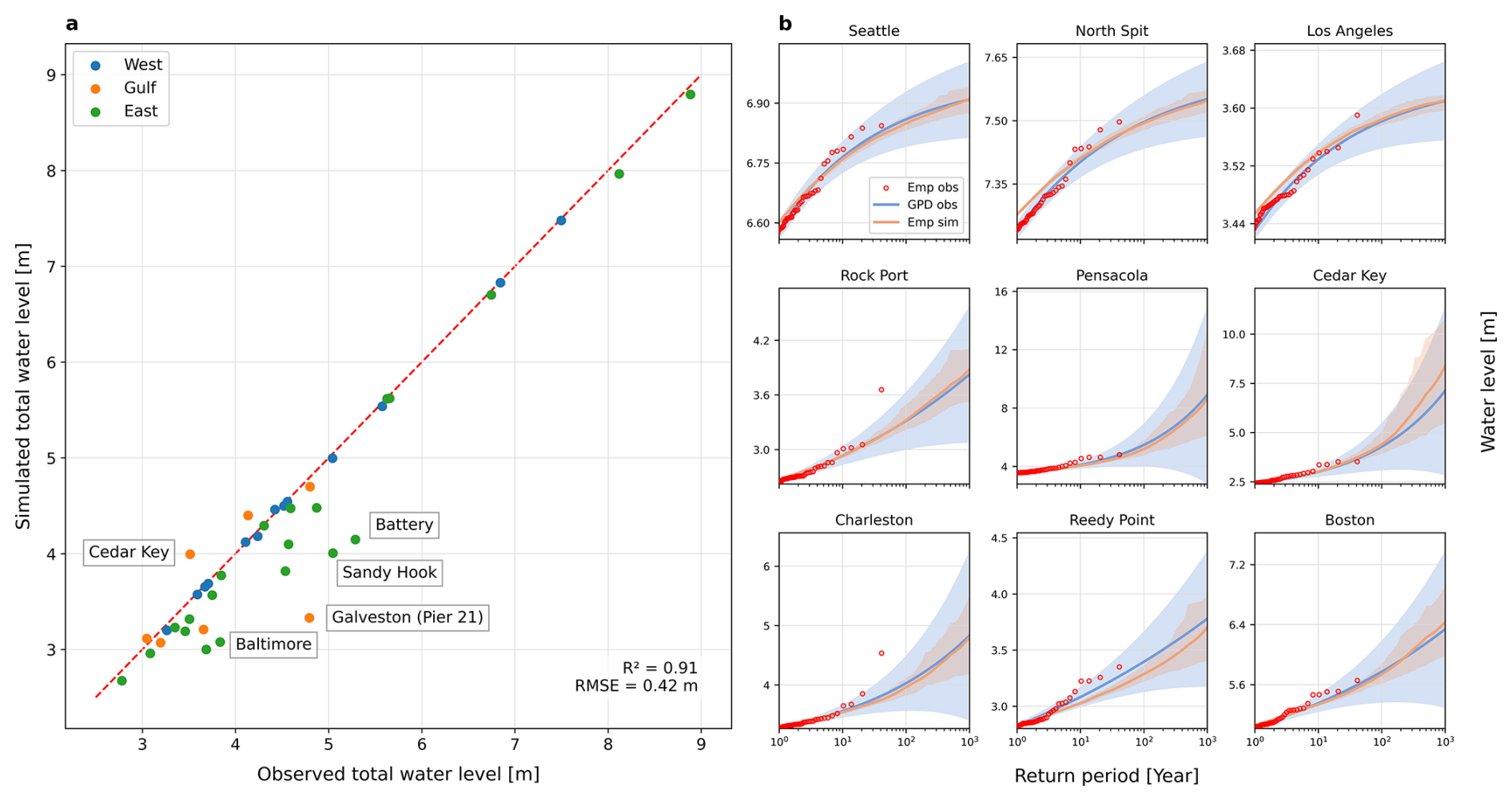
Figure 3 Validation of the generated synthetic coastal water levels. (a) Maximum observed versus simulated peak total water levels over a 41 year period at tidal gauges on the West coast (blue), Gulf of Mexico (orange), and East coast (green). The maximum observed peaks are extracted from the 41 year observations, while the simulated peaks refer to the median of total water levels from 250 random model samples of 41 years length. The red dashed line represents the identity (1:1) line. (b) Comparison between observed and simulated water level return periods for nine selected gauges (three per coast; see the locations in Fig. 1). Red dots are the empirical return periods from observed peak water levels, while blue curves represent the return periods from the GPD fit to the observations. Orange curves refer to the empirical estimates from the 10 000 year simulation. Shaded areas are the confidence intervals corresponding to the 5th and 95th percentiles.

3 Results and Discussions

3.1 Validation of simulated stochastic event sets

In Fig. 3, we show the validation results on the generated stochastic coastal water levels. Figure 3a compares the maximum simulated water levels against observations over a 41 year period for all 41 tidal gauges along the US coastlines used in this study. Results show that the simulated 41 year maximum water levels show good agreement with observations, with an overall coefficient of determination (R²) of 0.91 and a root mean square standard error (RMSE) of 0.4 m across all the gauges. The highest agreement is found at gauges on the West coast (blue). On the Gulf of Mexico (orange) and East coast (green), our model is found to underestimate the 41 year maximum water level for some gauges such as Battery, Sandy Hook, and Galveston (Pier 21), while the maximum water level is overestimated at Cedar Key. These misestimations are likely caused by the different approaches for estimating maximum water levels. The observed maximum water levels over a 41 year period may have a return period of larger than 40 years according to the extreme value analysis (e.g. see the water level comparison for Rock Port and Charleston in Fig. 3b). However, the obtained values, based on many realisations of 41 year water levels from the stochastic set, are approximately identical to the estimated 1-in-41 year water level. This case typically occurs at gauges in TC-prone areas. Due to the stochastic nature of TCs, observation records of a limited length, such as 41 years in this study, may contain too few TCs that made landfall to drive a good fit of extreme distributions to robustly estimate water level return periods (Dullaart et al., 2021).

Figure 2b compares the water level return periods estimated from the stochastic events (orange) and observations (blue) at nine randomly selected gauges (three per coast). The return periods calculated from simulated water levels correspond well with those derived from observed data, with narrower confidence intervals associated with the former mostly located within the confidence bounds associated with the observational data. This indicates that our approach can simulate water levels close to the marginal distributions of the observations with greater confidence, especially for high return periods. For North Spit and Los Angeles, our approach overestimates the water levels for relatively low return periods compared to estimated return levels using observations, which may be due to the sampling procedure used to identify spatially joint events. As this process tends to pair the peaks of the primary variable with maximum values of the remaining variables within a lagged window, the dependence structure may be overestimated and therefore higher values are generated.

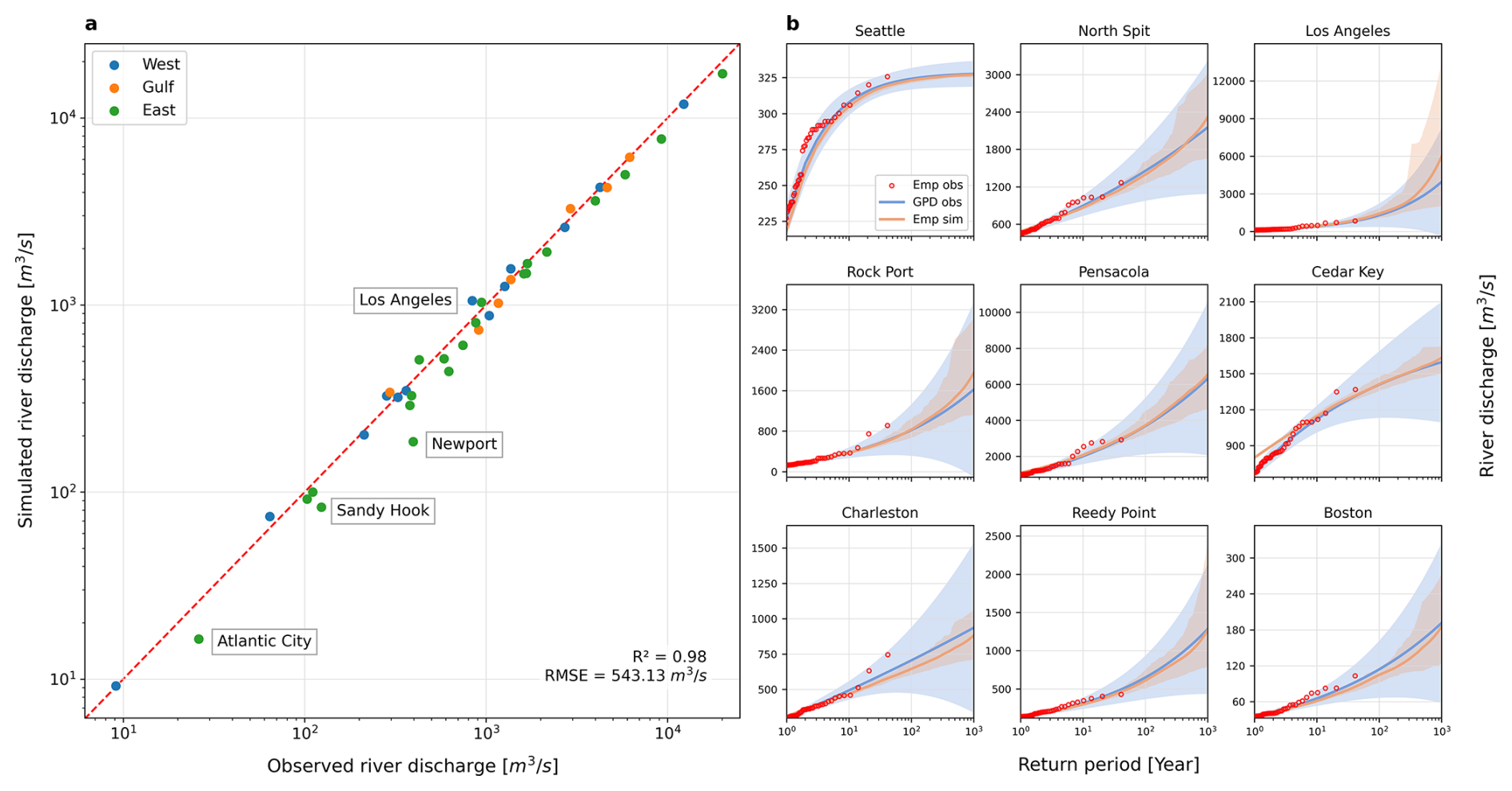
Figure 4 Validation of the generated synthetic river discharges. (a) Maximum observed versus simulated peak river discharges over a 41 year period at paired river stations on the West coast (blue), Gulf of Mexico (orange), and East coast (green). The maximum observed peaks are extracted from the 41 year observations, while the simulated peaks refer to the median of river discharges from 250 random model samples of 41 years length. The red dashed line represents the identity (1:1) line. (b) Comparison between observed and simulated water level return periods for the nine stations (paired with the nine coastal gauges; see the locations in Fig. 1). Red dots are the empirical return periods from observed peak water levels, while blue curves represent the return periods from the fitted GPD using these observations. Orange curves refer to the empirical estimates from the 10 000 year simulation. Shaded areas are the confidence intervals corresponding to the 5th and 95th percentiles.

Compared to total water levels, we find higher agreement between observed and simulated maximum river discharge over a 41 year period at all stations, see Fig. 4a. The coefficient of determination (R²) is 0.98 and the root mean square standard error (RMSE) is 511 m³ s⁻¹ across all stations. Figure 4b shows good correspondence between the return periods estimated from the stochastic events and observations for the river stations paired with the nine selected tidal gauges. At most stations, the simulated stochastic return levels show a narrower confidence interval. Overall, these validation results show that our approach can generate a much longer set of spatially joint events with similar marginal distributions compared to historical observations.

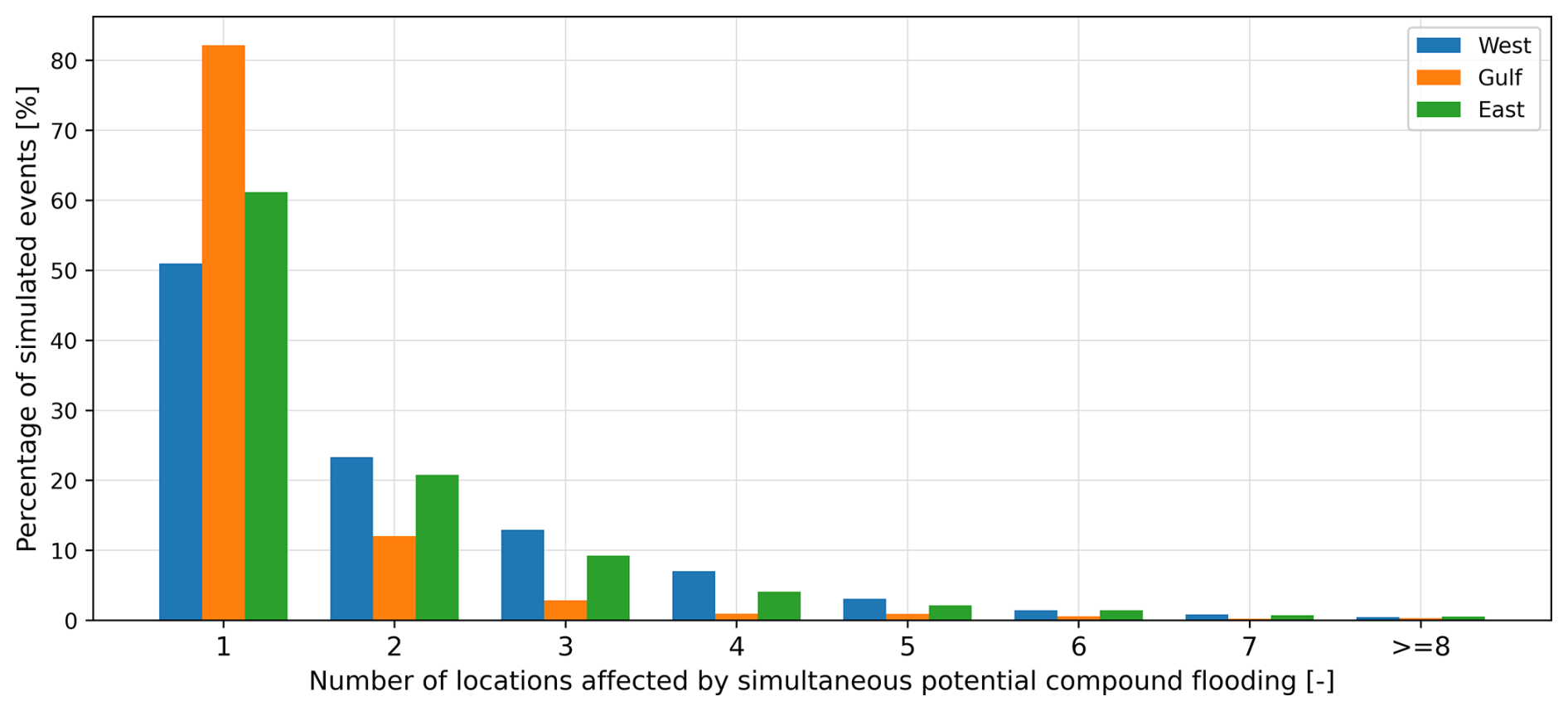
Figure 5 Event percentage diagram with the number of locations affected by simultaneous potential compound flooding for the West Coast, Gulf of Mexico, and East Coast. Potential compound flooding is defined by events where both total water level and river discharge exceed their respective 99th percentiles. Over the 10 000 year simulation period, the total number of potential compound flooding events is 24 086, 15 540, and 28 635 for the West, Gulf, and East coasts, respectively.

3.2 Frequency analysis of simultaneous potential compound flooding with the number of affected locations

Figure 5 shows the percentage of simulated events that may potentially cause compound flooding, categorised by the number of affected locations for the US coastal regions. These events are those with both total water level and river discharge exceeding the respective 99th percentiles. Our analysis reveals that the Gulf coast shows the highest frequency of localised compound flood events among the three US coasts, with over 82 % of all potential events affecting only a single location. Nevertheless, it is still likely (around 12 %) that potential compound flood events may affect two locations on the Gulf coast, while events that may affect more locations become increasingly rare (e.g. less than 3 % for three locations and 3 % for more than three locations). In contrast, the west coast shows higher frequencies of widespread potential compound flooding. For example, about 50 % of the events may result in potential compound flooding at one location while the chances of affecting multiple locations are 23 % for two locations, 13 % for three locations, 7 % for four locations, and 3 % for five locations. The east coast shows slightly lower frequencies of potential compound flooding events affecting multiple locations. The frequency of events affecting a single location is 61 %, followed by 21 %, 9 %, and 4 % for two, three, and four locations, respectively.

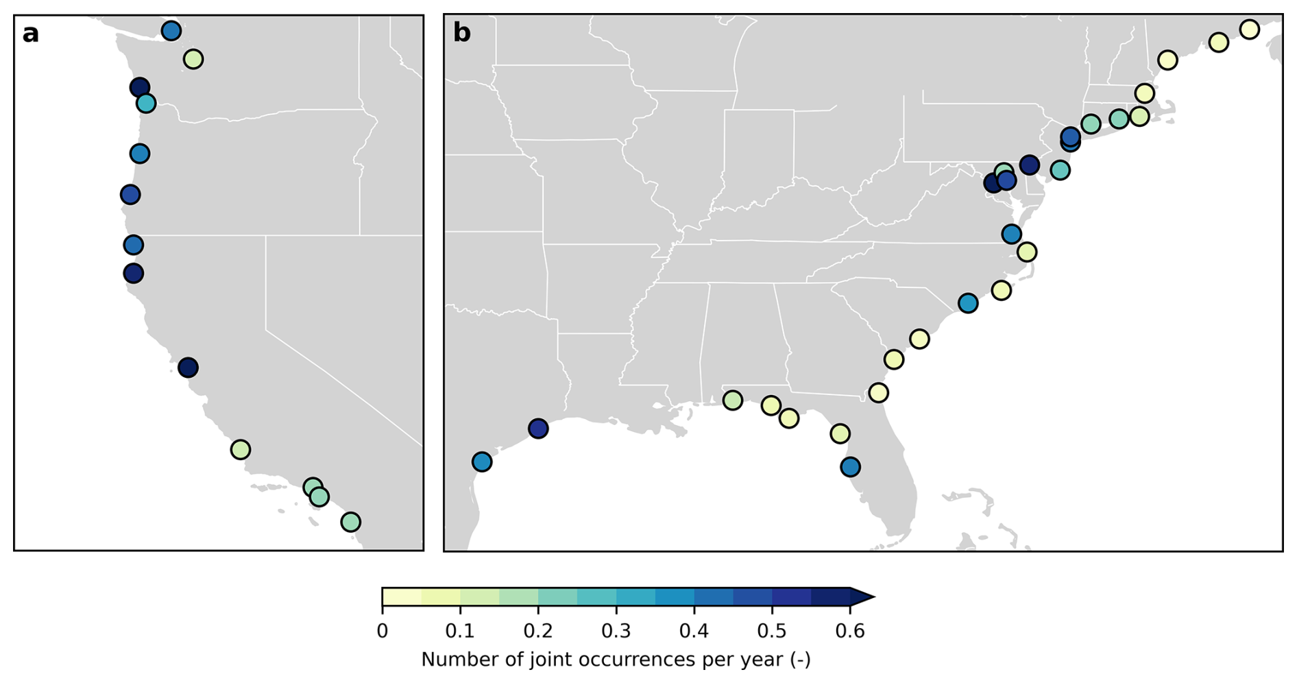
Figure 6 Number of joint occurrences per year between extreme total water levels and river discharges from simulated 10 000 year event sets for (a) the West coast and (b) the combined Gulf of Mexico and East Coast. Joint occurrences are defined for events where both water level and river discharge are above the 99th percentile threshold. The state borders are marked in white.

3.3 Joint occurrence of extreme sea levels and river discharges at individual locations

We first assess the compound flooding potential at individual locations based on the annual number of joint occurrences of total water level and river discharge above a specific threshold. Figure 6 shows the result using a threshold equivalent to the 99th percentile of the 41 year total water level and river discharge time series. The regional patterns of compound flooding potential largely align with those reported in previous studies (e.g. Couasnon et al., 2020; Ghanbari et al., 2021; Ward et al., 2018). For example, most locations on the US west coast show a high compound flooding potential, with an annual number of joint occurrences exceeding 0.3. This high potential is associated with the interplay between synoptic weather systems (e.g. ETCs) and regional orographic features, which causes simultaneous high storm surge and intense precipitation (Couasnon et al., 2020). These storm surges elevate the total water level, and the intense rainfall results in high river discharges in a short time as most river basins on this coast are relatively small and steep (Ward et al., 2018). At a few locations such as Seattle, Port San Luis, Santa Monica, and La Jolla, the compound flooding potential is relatively low and the annual number of joint occurrences is typically smaller than 0.2. The dependence between riverine and coastal drivers in these locations is found weak or statistically insignificant by previous studies. For example, Ward et al. (2018) found weak dependence between river discharge and skew surge at La Jolla, while Ghanbari et al. (2021) confirmed independence between total sea level and river discharge at Seattle and Santa Monica.

For the Gulf of Mexico, both stations on the western part show a high compound flooding potential with an annual number of joint exceedances of 0.38 and 0.53 for Rock Port and Galveston, respectively. However, the eastern part except St. Petersburg has a much lower joint exceedance value. This regional difference is due to seasonal patterns in river discharge and storm surge characteristics. High storm surges/sea levels on the Gulf coast are often driven by hurricanes (i.e. TCs). For the western part of this coast, maximum river flows also occur during hurricane seasons, while the river flow on the eastern part is often at its largest between late winter and early spring (Berghuijs et al., 2016).

The eastern coast of the US has a more complex spatial pattern of compound flooding potential with varying annual numbers of joint occurrences. For the southeastern coast, a low joint occurrence number (< 0.1) of total water level and river discharge is found for most locations except Wilmington. Although statistical dependence is found for these locations by other studies (e.g. Ghanbari et al., 2021; Ward et al., 2018), the dependence coefficient Kendall τ is generally low (e.g. ranging from 0.1–0.2 in Ghanbari et al., 2021)). The low annual number of joint occurrences may also be contributed to by the sampling method, which is based on automated thresholds in this study. For most locations on the southeastern coast, the identified thresholds are relatively high (see Table S2), which leads to much fewer sampled events from observations (see Fig. S2) and further a much smaller number of generated stochastic events. For the northeastern coast, we find a high compound flooding potential for the mid-Atlantic region while locations at the far northeastern coast generally show low compound potential. These results largely agree with previous findings (e.g. Wahl et al., 2015; Ward et al., 2018). On the eastern US coast, it is known that TCs can drive concurrent high storm surge and precipitation (Wahl et al., 2015). However, other mechanisms such as snow melt and convective storms that can generate riverine floods are also at play (Berghuijs et al., 2016), which could explain the regional difference in the compound flooding potential between the southern and northern parts.

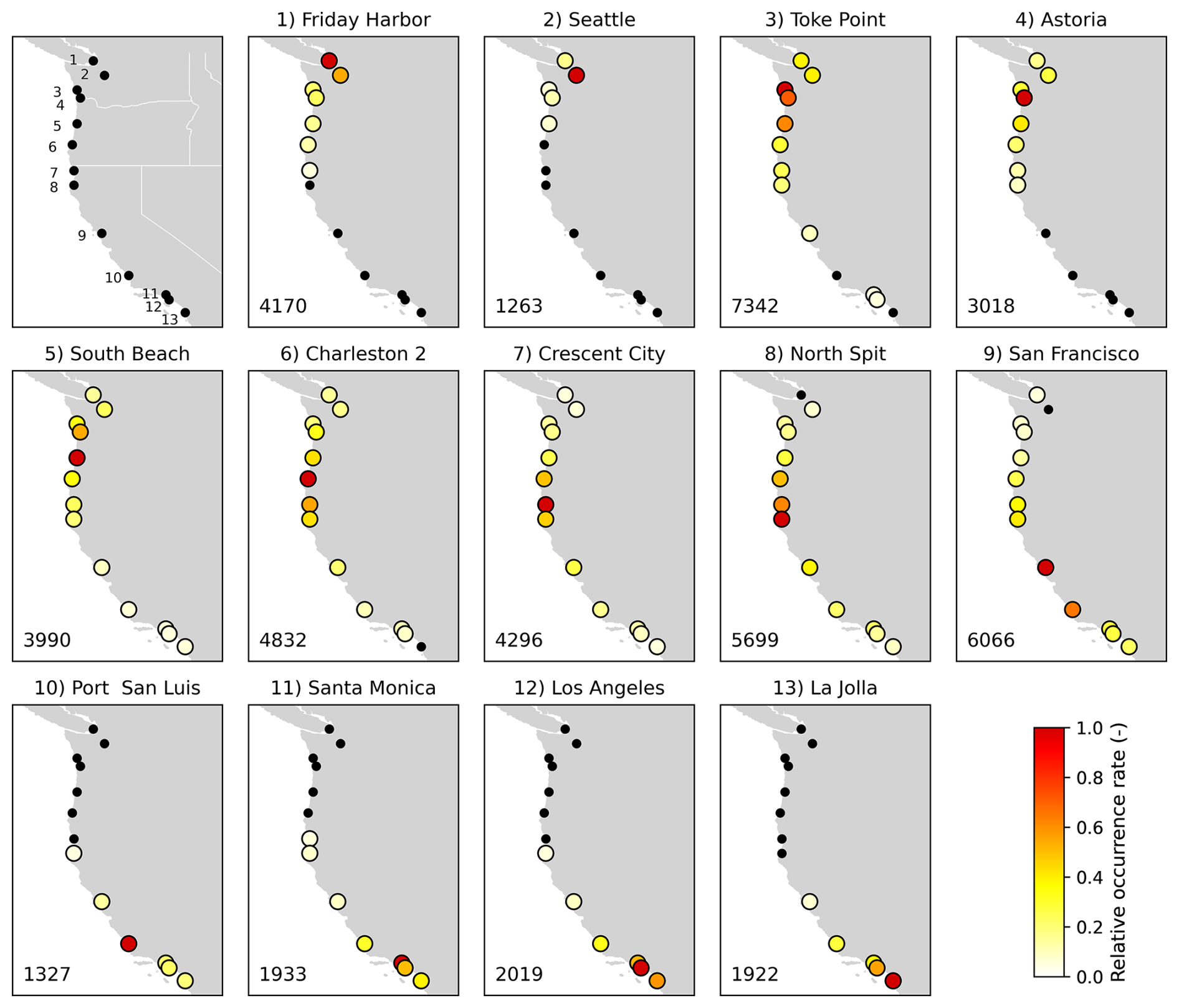
Figure 7 Relative occurrence rate of potential compound flooding at individual locations given potential compound flooding occurs at a primary location for the West Coast. The top-left panel shows the individual locations and the state borders are marked in white. Potential compound flood events are defined by events with both total water levels and river discharges exceeding the 99th percentile threshold. Small black solid circles refer to the relative occurrence rate lower than 0.05, and the number on the lower left corner of each subplot represents the total number of stochastic events with compound flooding potential at the primary location from the 10 000 year simulated event set.

3.4 Joint occurrence of extreme sea levels and river discharges across multiple locations

Moving from assessing compound flooding potentials at individual locations, we then assess the likelihood of simultaneous compound flooding arising across different locations. Figure 7 maps the relative occurrence rate of potential compound flood events at individual locations on the West coast of the United States, given the location of interest is experiencing an event with compound flooding potential. Here potential compound flood events are defined as events with both total water level and river discharge exceeding the 99th percentile. Results show that for the west coast, when a given location sees potential compound flooding, other locations are likely to experience potential compound flooding simultaneously. As one may expect, the relative occurrence rate shows asymptotic patterns across space: These rates are relatively high at locations near the primary location and start to decrease when the distance increases. For example, when a potential compound flood event occurs in Seattle, the chance that Friday Harbor is also affected is relatively high (0.54) while the joint rates for other locations are much lower (e.g. Toke Point: 0.39, Astoria: 0.27, Charleston: 0.16). At most locations, a relatively high joint occurrence rate (> 0.5) can be observed at one or two nearby locations. However, there are a few locations where three nearby locations show a high relative occurrence rate; this is case for Astoria, Crescent City, and Los Angeles.

We also observe two clustering patterns where more than two locations show mutually high relative occurrence rates. The first cluster is Charleston – Crescent City – North Spit; the relative occurrence rates for the other two locations are (1) 0.50 and 0.51, (2) 0.56 and 0.62, and (3) 0.47 and 0.40 given each of these three locations experience potential compound flooding. The second cluster covers the southwestern US coast (Santa Monica – Los Angeles – La Jolla). These clusters correspond with clustering results of storm surges (Enríquez et al., 2020) and total water levels (Li et al., 2023) based on in-depth statistical analyses. This indicates that synoptic weather events (i.e. ETCs on this coast) may be responsible for large-scale compound flooding at these locations.

To assess the sensitivity of the results to different thresholds for identifying potential compound flood events, we also apply varying thresholds equivalent to 1 and 2 year return levels, see Figs. S4 and S5. To maintain consistency, these varying thresholds are only applied for the primary location while the 99th percentile is used for the remaining locations on the west coast. We restrict this analysis up to 2 year return levels because the number of identified stochastic events will be very small when applying higher thresholds, and the further quantification of relative occurrent rates would be very biased based on such few events. We find similar patterns of the relative occurrence rates for different thresholds. With increasing thresholds, these relative occurrence rates become significantly higher. This is primary because larger storms are expected to have a greater spatial footprint and may therefore affect more locations.

For the Gulf of Mexico, we find lower relative occurrence rates of potential compound flooding for most locations. This shows a weak spatial correlation of compound flooding potential between locations, suggesting that compound flooding may occur at a local spatial scale on this coast. The reasons for this may be twofold. First, TCs are responsible for the majority of compound flood events on this coast (Lai et al., 2021); although TCs can cause more intense storm surge and rainfall, they have a smaller spatial footprint compared to ETCs (Dullaart et al., 2021). This is especially the case for the western Gulf coast (i.e. Rock Port and Pier 21) where the relative occurrence rate is 0.18 and 0.13 given each of these two locations sees a potential compound flood event in turn. Despite this, there are a few historic TC events, such as Hurricane Harvey, that resulted in compound flooding in both locations. Second, the eastern Gulf coast has a low compound flooding potential as extreme storm surge and high river flow typically occur in different seasons (Ward et al., 2018). Therefore, compound flooding is unlikely to arise at different locations.

On the East Coast, the relative occurrence rate of compound flooding potential shows mixed patterns. Both southern and northern parts show a weak spatial correlation of compound flooding with low relative occurrence rates, which could be associated with the low compound flooding potential in these regions. For the central part (between Swell Point to Newport), more than 50 % of the locations show a relatively low joint occurrence rate of potential compound flooding (< 0.4) for the remaining locations. Four locations, namely Swell Point, Annapolis, Sandy Hook, and Battery show a relatively high joint occurrence rate (> 0.4) at one nearby location. Baltimore shows the highest spatial correlation of compound flooding potential with other locations: Two nearby locations Washington and Annapolis show a high relative occurrence rate of 0.44 and 0.48; Swell Point and Reedy Point has a rate of 0.16 and 0.25 while the remaining locations show a lower occurrence rate (< 0.1). Compound flooding on the US east coast can be triggered by both TCs and ETCs, and the relative contribution of these two weather events varies spatially, which may correlate to the regional differences of spatial correlation of compound flooding potential.

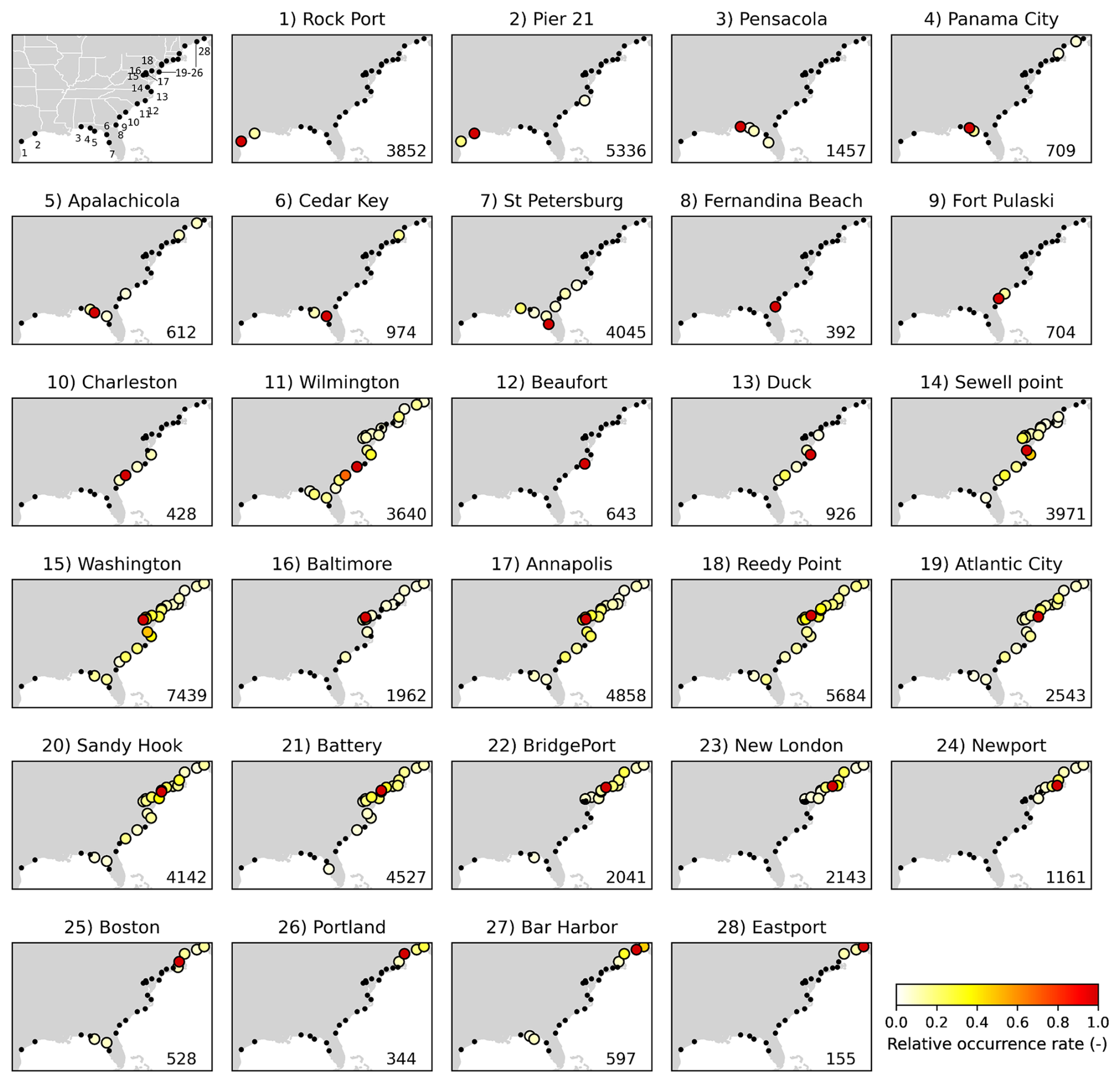
Figure 8 Relative occurrence rate of potential compound flooding at remaining locations given potential compound flooding occurs at a primary location for the combined Gulf of Mexico and East Coast. The top-left panel shows the individual locations and the state borders are marked in white. Potential compound flooding is defined by events with both total water levels and river discharges exceeding the 99th percentile. Small black solid circles refer to the joint occurrence rate lower than 0.05, and the number on the lower left corner of each subplot represents the total number of stochastic events with compound flooding potential at the primary location from the 10 000 year simulated event set.

We note that some relative occurrence rates of compound flooding potential show correlations between locations that are far way. For example, when Panama City sees a potential compound flood, Beaufort and Portland show a relative occurrence rate of 0.15 and 0.09, respectively (see Fig. 8). Other similar instances can be found for several locations (e.g. Boston and Bar Harbour) on the northeastern coast which show a small relative occurrence rate at locations on the Gulf coast. These correlations can be driven by the storm events that make a landfall on the Gulf coast and then travel into certain areas (e.g. the Carolinas) on the East coast. Prime examples of such events are Hurricane Idalia and Tropical storm Eta. On the other hand, these correlations can be spurious due to the applied time lags in the sampling process. A ± 3 d lag both spatially and between total water level and river discharge at individual locations can result in a sampled event of up to 13 d. This long duration may unintentionally correlate individual potential compound floods across multiple locations.

3.5 Relative frequency contributions of different types of events at other locations

Compound flooding may occur when only one driver is extreme. It is therefore important to estimate the simultaneous joint probability of different types of flood events from exceedances over either coastal or riverine flood threshold. When a location experiences a potential compound flood event, we assess the relative frequency contributions of different types of events at other locations. We identify four types of events: (1) compound where both drivers exceed the respective thresholds, (2) coastal driven where only total water level exceeds the threshold, (3) river driven where only river discharge exceeds the threshold, (4) non-extreme events where neither of the drivers exceeds the threshold. To keep consistent, we use the 99th threshold for both total water level and river discharge at all locations.

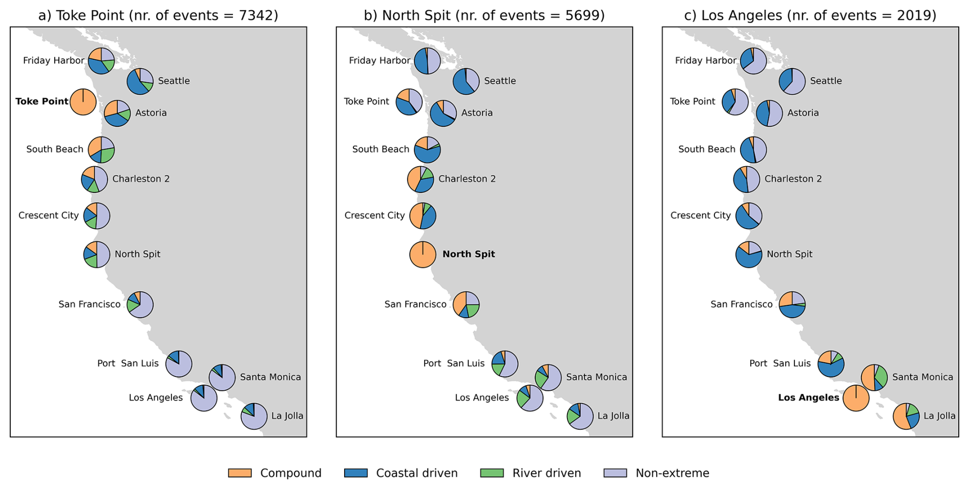
Figure 9 Relative frequency of different types of events given potential compound flooding occurs at a primary location for (a) Toke Point, (b) North Spit, and (c) Los Angeles on the US West Coast. Potential compound flood event (orange) is defined for events with both total water levels and river discharges exceeding the 99th percentile. The total number of simulated compound events at the primary location is indicated in the title of each panel. Blue refers to coastal driven events where only the total water level exceeds the 99th threshold, while green refers to river driven events where only the river discharge exceeds the 99th threshold. Purple refers to non-extreme events where neither of the drivers exceeds the threshold.

Figure 9 shows the relative frequency of these different types of events, i.e. compound (orange), coastal-driven (blue), river-driven (green), and non-extreme events (purple), for three selected reference locations with a relatively high compound flood potential on the West Coast. Results for other locations on this coast can be found in Figs. S8–S10. Note that the relative frequency of compound events (orange) is the same as the relative occurrence rate shown in Figs. 7 and 8.

At all three locations, the likelihood of simultaneous extreme events at other locations is high, when the primary location sees a potential compound flood event. For example, the relative frequency of extreme events (river, coastal or compound) is higher than 0.5 at six other locations between Friday Harbor and North Spit when Toke Point experiences a potential compound flood (Fig. 9a). Similarly, this high frequency of extreme events is seen at eight other locations when both North Spit (Fig. 9b) and Los Angeles (Fig. 9c) are the reference location. In most cases, the relative frequency contribution of coastal-driven events is higher compared to the respective contribution of river-driven events. This may suggest that total water levels exhibit stronger spatial dependence than river discharges at those locations selected in this study. The stronger dependence of total water levels may stem from the high tide events as the spring and neap tides occur at approximately the same time everywhere along the coastline. On the contrary, the correlation between high river discharges may not be fully captured by using a 3 d lag between locations as used in this study.

4 Limitations and recommendations

Our framework presents an advancement over the traditional large-scale statistical dependence assessment of compound flooding drivers, as it accounts for the spatial dependence of different drivers. However, several aspects of our framework could be further improved. Firstly, our analysis is based on observed data that may be biased towards a few locations. For example, no station combinations are selected for the central Gulf coast or for most parts of the coastline of Florida due to the relatively short time-span of the gauge records at these locations. Some of the selected station combinations suffer from long data gaps which are later infilled using simultaneous data from nearby locations. This may unintentionally increase the correlation between these locations. Therefore, future studies are recommended to apply our framework to modelled time series of flood drivers (e.g. storm surges (Muis et al., 2023) and river discharges (Harrigan et al., 2020)). This would improve the assessment of spatial correlation of potential compound flooding at multiple locations, although these models cannot fully resolve the TC activities.

Secondly, our framework is limited to extreme total water level and river discharge. However, other drivers may also contribute to compound flooding. For example, waves were the dominant contributor to inundation along a stretch of coastline during Hurricane Florence (Leijnse et al., 2025). In some regions with high connectivity between ground and surface water hydrology, groundwater level is a paramount driver to consider in the compound flooding assessment (Jane et al., 2020). River discharge is used to represent the riverine component for compound flooding; however, precipitation can be the predominant driver for compound flooding in some regions (Sohrabi et al., 2025) and should be considered in the dependence analysis. A future version of our framework is therefore recommended to include relevant drivers depending on the locations, thereby providing more robust boundary conditions for assessing the inundation and risk of compound flooding.

Our results are based on a large set of stochastic events specified by spatiotemporal limits. In this study we define events for two areas: (1) the West Coast; and (2) the combined Gulf and East coasts. Given these relatively large areas, spurious correlations are observed for locations that are far away from each other. For example, when Panama City sees a potential compound flood, Beaufort and Portland show a non-negligible relative occurrence rate of potential compound flooding (Fig. 8). An improvement for this would be to define the events for the identified clusters of storm surges (Enríquez et al., 2020) and extreme sea levels (Li et al., 2023). Moreover, these spurious correlations may also stem from the applied time lags between flood drivers and between locations. In this study, a 3 d window for both factors would result in a sampled event with a time window of ranging from 7 to 13 d. Although the effects of time lags are found negligible on the dependence between different drivers at individual locations (Camus et al., 2021), a long time window may unintentionally correlate individual potential compound floods across different locations. Therefore, future work is recommended to use different lags and to further assess the sensitivity to these assumptions.

In regions where compound flooding can result from multiple synoptic weather patterns (e.g. TCs and ETCs) and hydrological processes (e.g. snowmelt and convective rainfall), different generation mechanisms may produce distinct dependence structures between flood drivers (Kim et al., 2023). To capture these mixed-population effects, our stochastic event generation could be improved by distinguishing events based on their generation types rather than combining all events into a single population (c.f. Maduwantha et al., 2024). Such event stratifications require long and continuous time series of flood drivers (e.g., the 122 year observations used in Maduwantha et al., 2024), which may not be available for large-scale analyses. Future work could therefore consider using additional datasets for a long time series synthetic TCs (e.g. Bloemendaal et al., 2020) and ETCs derived from seasonal forecasting data (e.g. Benito et al., 2025), as well as hydrological data generated by stochastic weather generators (e.g. Falter et al., 2015; Ullrich et al., 2021).

The final limitation of our study is the identification of the compound events using “and” hazard scenarios where both total water levels and river discharges exceed a range of thresholds. In reality, compound flooding may occur even when neither of these two drivers is extreme. Therefore, a more realistic identification of compound events could be based on impact thresholds rather than hazard thresholds (Ghanbari et al., 2021). Such impact thresholds have been established for the United States, including impact thresholds for both coastal (Sweet et al., 2018) and riverine flooding (Cosgrove et al., 2024). These thresholds are used for forecasting purposes, enhancing public safety, and supporting actions to improve preparedness. However, these thresholds are not available at all station combinations used in this study, which is the further reason that we use a range of hazard thresholds for identifying potential compound flood events.

5 Conclusions

We provide the first assessment of spatial correlation of potential compound flooding from extreme sea levels and river discharges at 41 station combinations on the US coasts. Our results are based on a large set of stochastic events simulated using a multivariate conditional dependence model. The validation results show that our stochastic events can well capture the observed dependence structure between total water levels and river discharges across multiple locations. Our assessment of compound flood potentials at individual locations largely agrees with previous findings. Our frequency analysis of potential compound flood events across locations shows that potential compound flooding is likely to affect multiple locations. On the west coast of the US, around 50 % of potential compound events may arise at more than one location simultaneously. Less than 30 % of potential compound flooding may affect multiple locations on the East coast, while the frequency of widespread compound flooding is low on the Gulf coast. Our analysis of relative occurrence rates reveals that potential compound events exhibit strong spatial correlation particularly among neighbouring locations along the US West coast. Two clusters where multiple locations show mutually high joint occurrence rate of potential compound flooding are identified: (1) Charleston – Crescent City – North Spit; and (2) Santa Monica – Los Angeles – La Jolla. In contrast, the Gulf Coast shows the weakest spatial correlation while the East Coast presents mixed behaviour with moderate spatial dependence in the central region and weaker spatial dependencies for the remaining locations. These spatial patterns may be associated with the major driving weather patterns of compound flooding where ETCs have a larger spatial footprint and are more likely to cause widespread events compared to TCs.

Our results advocate for considering spatial dependence in compound flood risk assessment, especially for regions prone to large-scale synoptic weather patterns, such as Europe and eastern Asia. While the focus of this study is on the US coasts, the methodologies developed in this study are readily transferable to other coastal and estuarine regions facing the challenges of compound flooding. Our stochastic event sets can be used as boundary conditions for coupled hydrologic-hydraulic models for simulating the surface inundation and assessing flood risk. Our results of relative contributions of different types of events along the coastlines can facilitate more effective trans-regional flood risk management through better flood adaptation, planning, and emergency response in low-lying coastal catchments.