Assessment of seismicity and risk from gas injection in the Groningen gas field

Production of natural gas from the Groningen gas field in the Netherlands has led to earthquakes, the societal impact of which has ultimately led to the decision to cease all gas production from the field starting October 2023. Seismicity is expected to continue for some time, even after production has stopped, at least in part because of the existing pressure gradients in the field and the time that it will take for gas to re-distribute and pressure to equilibrate. We investigate the possibility to reduce the seismicity by means of gas injection. We employ a dedicated model chain previously developed to model gas production, induced seismicity, and associated hazard and risk. The model chain was adapted to support modelling of pressure increases associated with gas injection, and to account for the effects of reservoir cooling when relatively cold gas is injected. Several injection scenarios are considered that are based on realistically feasible total injection gas volumes. Additional scenarios are designed to provide useful insight into fundamental mechanisms. The scenarios are compared to a no-injection reference case to be able to identify and quantify beneficial effects. The results indicate that reductions in seismicity can be achieved in all scenarios and that these reductions could be substantial also for relatively modest volumes of injection gas. The results also show that benefits may be lost if injection is stopped before reservoir-wide equilibration has been achieved. We discuss also some limitations of the model chain and highlight possibilities to deploy more targeted injection schemes.

1 Introduction

The Groningen gas field in the Netherlands is the largest onshore natural gas field in Europe. It was discovered in 1959 and production started in 1965. Since 1991, the production of gas from the field has led to seismic events, the societal impact of which has ultimately led to the decision to cease all gas production from the field from October 2023 onwards. The generally accepted understanding is that the seismicity is largely the consequence of compaction at reservoir level, caused by lowering of the gas pressure in the reservoir, leading in turn to critically stressed faults and seismic fault slip. It is expected that this form of induced seismicity will continue for some time also after production has stopped. There are two main reasons for this. (1) The existing spatial pressure gradients in the field will cause the gas to re-distribute, leading to pressure increases in some parts of the field and pressure decreases in other parts of the field. These decreases in pressure could cause further compaction and therefore potentially new seismic events (TNO, 2022). (2) The compaction response to pressure changes is expected to contain a time-dependent component, which leads to ongoing compaction even when local pressures are stable (Aben et al., 2025; Pijnenburg et al., 2019).

In this manuscript, we focus on the first mechanism. Since pressure equilibration is expected to contribute to future seismicity, it stands to reason that a more favourable pressure state (one that would lead to a reduction in seismicity) could be actively created by strategic injection of gas. The objective of injection would be to reduce or prevent pressure decline in crucial parts of the field, leading to a more stable stress state and thereby less seismicity. Pressure maintenance by fluid injection can therefore be considered as a possible safety measure for the Groningen field, along with the ongoing reinforcement of buildings after the recent cessation of gas production. The idea of pressure maintenance was already considered in 2013 during the production phase as part of a study program by the operator (NAM, 2016) and independent research organizations (TNO, 2014, 2015a, b, c). These studies determined that gas injection is technically feasible and could help reduce the rate of pressure decline, or stabilize pressures. At that time, however, it was not yet possible to determine the impact of such measures on seismicity. Both the pressure maintenance studies and a recent study conducted in 2022 (Fugro, 2022) concluded that nitrogen (N₂) injection would be most effective (e.g. more so than CO₂ injection).

Induced seismicity effects have been associated with different types of subsurface operations, as classified by McGarr (2014). These include the injection of wastewater into deep formations (Ellsworth, 2013), the injection of CO₂ into oil reservoirs for enhanced recovery (Rubinstein and Mahani, 2015) or for permanent storage (Evans et al., 2012), hydraulic fracturing to stimulate production from low-permeable oil reservoirs or shale gas reservoirs (Warpinski et al., 2012) , and the development of enhanced geothermal systems (Evans et al., 2012; Zang et al., 2014). A general overview was provided by Foulger et al. (2018) that includes concepts for monitoring strategies and traffic-light systems. These works do not discuss technologies for actually reducing fluid injection-related induced seismicity, e.g., by advanced injection schemes (see e.g. Candela et al., 2022). Design of such schemes are believed to require detailed predictive understanding of hazard posed by induced earthquakes as influenced by the stress and pressure conditions at depth, the hydrogeologic framework, including the presence and geometry of faults, and the location and mechanisms of natural seismicity (Zang et al., 2019). The Groningen model chain for Seismic Hazard and Risk Assessment (SHRA) was developed exactly with this philosophy in mind (TNO, 2022). It has been the basis for discussions between operator and regulators during the final years of production from the Groningen field and continues to play an important role in monitoring and analysis of ongoing events in the field. In the seismic source model used within the model chain, which was originally designed to model the expected effects of gas production, seismicity is only possible at locations and times in the field where the gas pressure is decreasing. Since N₂ injection will cause an overall increase in the gas pressure, the pre-existing modelling framework is expected to model primarily beneficial effects of fluid injection. Any potentially negative effects caused e.g. by reservoir cooling, or by local development of tensile stresses due to high injection pressures, are not modelled. For the Groningen case, we do not expect significant effects of the pressure increase due to N₂ injection on seismicity for the following reasons: (1) The Groningen reservoir rock is very permeable, leading to modest near-well pore pressure increase when injecting, i.e. the near-well pressure is reasonably well represented by the large-scale reservoir simulations. (This is supported by analysis of our simulations, in which the bottom hole pressure of injection wells and the grid block average pressure of grid blocks with an injection well differ less than 0.1 MPa. We therefore do not expect local failure around the well due to the pressure increase.) (2) In the normal-faulting stress field of the Groningen gas field, pressure increase is expected to stabilize the faults (Van Wees et al., 2017). (3) Injection would be mainly aimed at stopping pressure decrease, rather than substantially increasing pore pressures compared to their present state. Mild pore pressure increase is already seen in some parts of the Groningen gas field for several years. In these areas, seismicity is largely absent, suggesting that the current source model actually captures the reservoir response to moderate pore pressure increase rather well.

Reservoir cooling, on the other hand, would be associated with a decrease in horizontal stress and associated potential destabilization of faults. The current source model is based on linear poro-elasticity. Hence, here we explore the theoretical foundations of linear poro-elasticity with thermal effects in conjunction with its implementation in the model chain, to further examine their combined impact on induced seismicity. In this work we apply the adjusted SHRA framework to a selected range of scenarios for the post-production period that include the injection of N₂ with the purpose of assessing the potential to reduce seismicity.

The remainder of this paper is structured as follows. We first review the main characteristics of the Groningen SHRA framework, including the individual model chain elements, and introduce extensions to model the effects of reservoir cooling due to injection of relatively cold gas. We then introduce a range of scenarios for gas injection that will be used to determine the possible benefits of such a remediation strategy. The results from the scenario evaluations are presented and analysed subsequently. We finalize this paper with a discussion and conclusions.

2 Methodology

In this work, the seismicity, seismic hazard, and seismic risk are modelled with the TNO Model Chain for Groningen (TNO, 2022), referred to in the following simply as the model chain. The model chain takes time series pressure grids resulting from reservoir simulations as input and produces probabilistic projections of both magnitude, timing and location of expected seismic events, ground motion distributions, and ultimately local personal safety risk associated with structural failure of buildings in the affected areas. We will here review the main modelling approaches adopted for these different stages of the model chain, introduce an extension to account for temperature effects, and discuss implications of all elements of the chain for assessment of the effects of gas injection. The overall workflow is illustrated in Fig. 1.

Figure 1 Schematic overview of the TNO Model Chain Groningen.

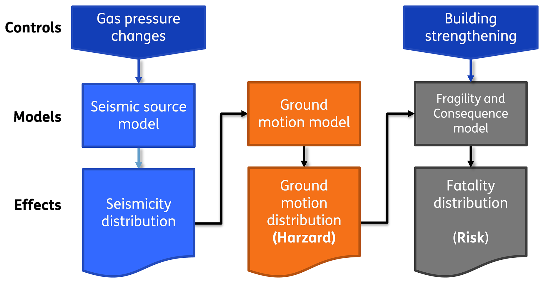
In this schematic, controls refer to input to the whole model chain that can be influenced by choices made by people. Gas pressure changes are the result of choices for production and injection rates, and for injection gas composition and temperature, and can be modelled with a reservoir simulator. The effects are the outputs simulated with the various model elements that may serve as inputs to the next model in the model chain.

The chain is probabilistic in nature, and deals with both aleatoric variability (e.g. the variation in ground motions at a given distance and magnitude) and epistemic uncertainty (e.g. uncertainty in the parameter controlling the variability in ground motion, uncertainty the maximum possible magnitude, and uncertainty in the building fragility parameters). Aleatory is accounted for by calculating model results in terms of probability distributions, rather than deterministic outcomes. Epistemic uncertainty is treated by including a logic tree (TNO, 2022).

In general, the spatial grids used in the various stages of the modelling are chosen such that further refinement does not lead to meaningful changes in the final hazard and risk results. A notable exception to this is the gas flow model, which was provided by the field operator NAM (see section on gas production modelling below). This model's spatial resolution was not studies or altered. However, given the relatively smooth spatial patterns associated with gas production in a high-permeability reservoir, we do not expect the model resolution of the reservoir flow model to be an important factor in the final modelling results.

2.1 Gas production and injection

Gas production modelling is not formally part of the model chain as originally documented in the TNO report (TNO, 2022), but since it is an integral part of the full workflow that is applied in this study we will include it here as part of the methodology description.

An Eclipse 100 (SLB, 2022) reservoir simulation model of the Groningen gas field has been developed by NAM, based on the existing in-house simulation model, and was made publicly available (Tummala et al., 2023). The model simulates dry-gas production from the Groningen gas field and from several neighbouring small fields between December 1955 and 1 January 2023. A review of the model revealed differences with historic measurements mostly at the western periphery of the field and for several small fields that are also included in the model but were not history matched. No fault multipliers are implemented in the released model. The following adjustments were made to the model for the purpose of this study. Fault multipliers were taken from Table 12-1 of the 2016 Groningen model release report (SGS Horizon, 2016). This resulted in somewhat sharper simulated pressure differences across the major boundary faults of the Groningen field, in closer agreement with the NAM in-house model and with historic pressure data. Production data for the period 1 January 2023 to 1 October 2023 were extracted from NLOG (http://nlog.nl, last access: 7 July 2026) and used to extend the simulation schedule up to the end-of-production.

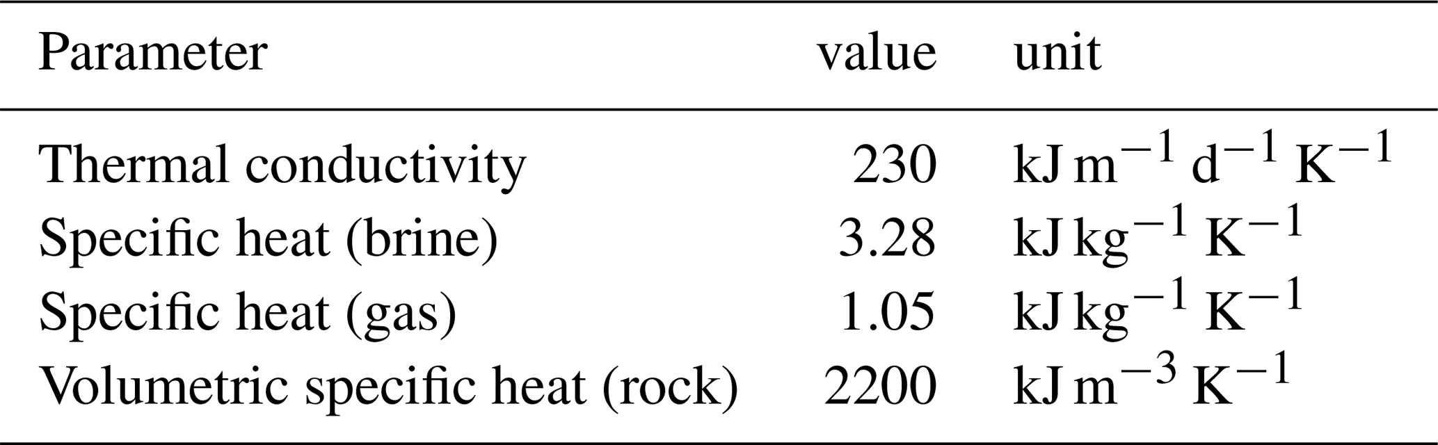
The Eclipse 100 simulator is based on a so-called black-oil formulation in which fluid phases water and (dry) gas are given bulk properties consistent with their composition. Individual molecular components of the gas are not explicitly distinguished, as would be done in a compositional simulator. It is therefore not possible with this model to simulate injection of a gas with properties that are different from the gas that is already present in the reservoir. Since the focus of this simulation study is primarily on the impacts of re-pressurization and cooling, we will assume that injected gas has the same properties as the natural gas present in the Groningen reservoir. The volumetric effects of gas composition were investigated in a separate experiment with a compositional simulator but are not reported here. Temperature was simulated using the Eclipse 100 TEMP option, which solves an energy balance equation after each time step that updates the pressure and saturation states. Initial reservoir temperature and specific heat values were specified, and an injection temperature of 10 °C as assumed (see Table A1 in Appendix A for parameter values used in this study).

2.2 Seismic source model

The Seismic Source Model (SSM) forecasts the spatial and temporal distribution of induced earthquakes, as well as their magnitudes, conditional on a production scenario. The seismic source model implementation is described in TNO (2022), which builds on peer-reviewed work (Bourne and Oates, 2017; Bourne et al., 2018). It combines a compaction model that calculates Coulomb stress changes from pore pressures changes and fault properties. This compaction model, and the spatial distribution of vertical reservoir compressibility parameter that, together with the pressure changes, controls the vertical strain is thoroughly calibrated on inversion of the subsidence bowl caused by the gas extraction (Bierman et al., 2015). This model is based on directly inverting the observed subsidence without assuming any prior knowledge of the reservoir rock physical properties and shows a good spatial and temporal match to the observed subsidence (Bierman et al., 2015). The stress changes are converted to a seismicity distribution (time, space and magnitude), that includes aftershocks based on a Epidemic-Type Aftershock Sequence (ETAS) model (Ogata, 1988, 1998). SSM parameters are calibrated using historic seismicity data using a probabilistic approach that results in a distribution of model weights, where each model is defined by a different combination of parameters.

2.3 Ground motion model

The Ground Motion Model (GMM) relates the earthquakes at depth to ground motions at the surface (Bommer et al., 2022a, b), and was specifically developed for the induced earthquakes in the Groningen region. The main outputs are horizontal spectral accelerations at different frequencies and return periods,. These are primarily of relevance for the integrity of infrastructure and buildings. The model incorporates information about the presence at depth of hard rocks and about the spatial variation in soft soil types through a zonation model with 160 zones. Output of the GMM are annual exceedance probabilities of spectral accelerations per grid point at the surface and constitute hazard.

2.4 Fragility and consequence model

The Fragility and Consequence Model (FCM), translates ground motions to building damage/collapse and the risk to people inside those buildings. It consists of a fragility model and a consequence model (Crowley and Pinho, 2020). The fragility model is implemented for 35 building types and calculates the probability of exceedance of various damage/collapse states for given ground motions. The consequence model describes the probability of a fatality (a single hypothetical person permanently present in or near the building dying) as a results of structural collapse of a building.

2.5 Extension of the seismic source model for temperature effects

We start by briefly reviewing the theory of linear poro-elasticity combined with thermal effects. Linear poro-elasticity describes the behaviour of fluid-saturated porous materials under small reversible deformation. It is based on principles such as conservation of mass, which ensures fluid balance within the pores, and conservation of momentum, which considers the balance of internal and external forces. The effective stress, according to Terzaghi's principle, is defined as the total stress minus the pore fluid pressure. Constitutive relations in this theory link stress σ and strain ε in the material, taking into account the interplay between the solid matrix and fluid pressure P_p.

The theory sets the basis for understanding more complex phenomena when additional factors like thermal effects are included. When thermal effects are incorporated, the theory extends to linear thermo-poro-elasticity, addressing the thermal expansion/contraction of the solid matrix due to spatio-temporal variations in the temperature. Thus, the system of equations in index notation describing linear poro-elasticity combined with thermal effects reads (Fjaer et al., 2008):

$$\begin{array}{}\text{(1)}& \begin{array}{rl}{\mathit{\sigma }}_{ij}=& {\displaystyle \frac{Ev}{(\mathrm{1}+v)(\mathrm{1}-\mathrm{2}v)}}{\mathit{\epsilon }}_{\mathrm{vol}}{\mathit{\delta }}_{ij}+{\displaystyle \frac{E}{\mathrm{1}+v}}{\mathit{\epsilon }}_{ij}+\mathit{\alpha }{P}_p{\mathit{\delta }}_{ij}\\ & +{\displaystyle \frac{E}{\mathrm{1}-\mathrm{2}v}}{\mathit{\alpha }}_{\mathrm{T}}\mathrm{\Delta }T{\mathit{\delta }}_{ij},\end{array}\end{array}$$

where E, v, α and α_T are the Young modulus, Poisson's ration, Biot's coefficient and linear thermal expansion coefficient, respectively. In the context of the model chain framework, ΔT is an input variable obtained from reservoir simulations that accounts for the spatio-temporal variations in the temperature field as fluid injection/production occur.

The seismic source model is based on uniaxial strain conditions, where strain is applied only in the vertical direction. This approach simplifies the material's response by focusing the analysis on stress and strain relations along the horizontal plane. Consequently, Eq. (1) is rewritten to reflect changes in vertical and horizontal stresses as follows:

$$\begin{array}{}\text{(2a)}& {\displaystyle }E{\mathit{\epsilon }}_{\mathrm{H}}=\mathrm{\Delta }{\mathit{\sigma }}_{\mathrm{H}}-v\left({\mathit{\sigma }}_{\mathrm{h}}+{\mathit{\sigma }}_{\mathrm{v}}\right)-\left(\mathrm{1}-\mathrm{2}v\right)\mathit{\alpha }\mathrm{\Delta }{P}_p-E{\mathit{\alpha }}_{\mathrm{T}}\mathrm{\Delta }T,\text{(2b)}& {\displaystyle }E{\mathit{\epsilon }}_{\mathrm{h}}=\mathrm{\Delta }{\mathit{\sigma }}_{\mathrm{h}}-v\left({\mathit{\sigma }}_{\mathrm{H}}+{\mathit{\sigma }}_{\mathrm{v}}\right)-\left(\mathrm{1}-\mathrm{2}v\right)\mathit{\alpha }\mathrm{\Delta }{P}_p-E{\mathit{\alpha }}_{\mathrm{T}}\mathrm{\Delta }T,\text{(2c)}& {\displaystyle }E{\mathit{\epsilon }}_{\mathrm{v}}=\mathrm{\Delta }{\mathit{\sigma }}_{\mathrm{v}}-v\left({\mathit{\sigma }}_{\mathrm{H}}+{\mathit{\sigma }}_{\mathrm{h}}\right)-\left(\mathrm{1}-\mathrm{2}v\right)\mathit{\alpha }\mathrm{\Delta }{P}_p-E{\mathit{\alpha }}_{\mathrm{T}}\mathrm{\Delta }T,\end{array}$$

where ε_H and σ_H refer to the maximum horizontal strain and stress respectively, and ε_h and σ_h are the minimum horizontal strain and stress. Under uniaxial strain conditions, ${\mathit{\epsilon }}_{\mathrm{H}}={\mathit{\epsilon }}_{\mathrm{h}}=\mathrm{0}$, and

$$\begin{array}{}\text{(3a)}& {\displaystyle }\begin{array}{rl}\mathrm{\Delta }{\mathit{\sigma }}_{\mathrm{H}}& =\mathrm{\Delta }{\mathit{\sigma }}_{\mathrm{h}}\\ & ={\displaystyle \frac{\mathrm{1}-\mathrm{2}v}{\mathrm{1}-v}}\mathit{\alpha }\mathrm{\Delta }{P}_p+{\displaystyle \frac{H(\mathrm{1}-\mathrm{2}v)(\mathrm{1}+v)}{(\mathrm{1}-v{)}^{\mathrm{2}}}}{\mathit{\alpha }}_{\mathrm{T}}\mathrm{\Delta }T,\end{array}\text{(3b)}& {\displaystyle }{\mathit{\epsilon }}_{\mathrm{v}}=-{\displaystyle \frac{\mathrm{1}}{H}}\mathit{\alpha }\mathrm{\Delta }{P}_p-{\displaystyle \frac{(v+\mathrm{1})}{(\mathrm{1}-v)}}{\mathit{\alpha }}_{\mathrm{T}}\mathrm{\Delta }T,\end{array}$$

Here, we assume Δσ_v=0, because the vertical stress remains constant due to the constant weight of the overburden layers. For convenience, Eqs. (3a) and (3b) are expressed in terms of the uniaxial compaction modulus H. The uniaxial compaction modulus H is a measure of the material's stiffness under uniaxial strain conditions. The formula for the uniaxial compaction modulus H in terms of Poisson's ratio v and Young's modulus E is derived from the relationship between stress and strain under uniaxial conditions:

$$\begin{array}{}\text{(4)}& H={\displaystyle \frac{E(\mathrm{1}-\mathit{\nu })}{(\mathrm{1}-\mathrm{2}v)(\mathrm{1}+v)}},\end{array}$$

This relation comes from the generalized Hooke's Law and reflects the effect of Poisson's ratio on volumetric strain under uniaxial loading.

In the context of the source model framework, the uniaxial compaction modulus is a spatially varying model parameter. In other words, the amount of strain for a given amount of pore pressure change is not spatially constant, due to the spatial heterogeneity of the reservoir rock's material properties. We deem it likely that this implies that the reservoir rock would also not respond homogeneously to a given change in temperature. Here, we relate the sensitivity of the vertical strain to temperature change (given by α_T) to the uniaxial compaction modulus H.

An important feature to pay attention to is the relationship between the material stiffness E and the thermal expansion coefficient α_T. Generally, the stiffer the material, the less it expands or contracts with temperature changes. This trend is primarily due to stronger atomic or molecular bonds in stiffer materials, which resist deformation under both mechanical and thermal stresses. There exists an inverse relationship between the thermal expansion coefficient (α_T) and Young's modulus (E) (Wachtman et al., 1961). This relationship is expressed in terms of the uniaxial compaction coefficient as follows:

$$\begin{array}{}\text{(5)}& {\mathit{\alpha }}_{\mathrm{T}}=a_{\mathrm{T}}/H,\end{array}$$

where a_T is a new model parameter that has to be calibrated within the seismic source model. Note that here, the Young's modulus E is included through H (Eq. 4). A prior range for this parameter can be defined based on the known range of α_T in Rotliegend sandstone rocks, and the range of values for H that are used in the current implementation of the seismic source model. Further calibration of the parameter a_T can be based on observations of seismicity (or lack thereof), in combination with actual cold fluid injection and non-isothermal reservoir modelling. Due to local historical water injection, some temperature changes are present in the history-matched reservoir model. Although they are limited, these temperature changes allow some initial calibration of a_T.

3 Injection scenarios

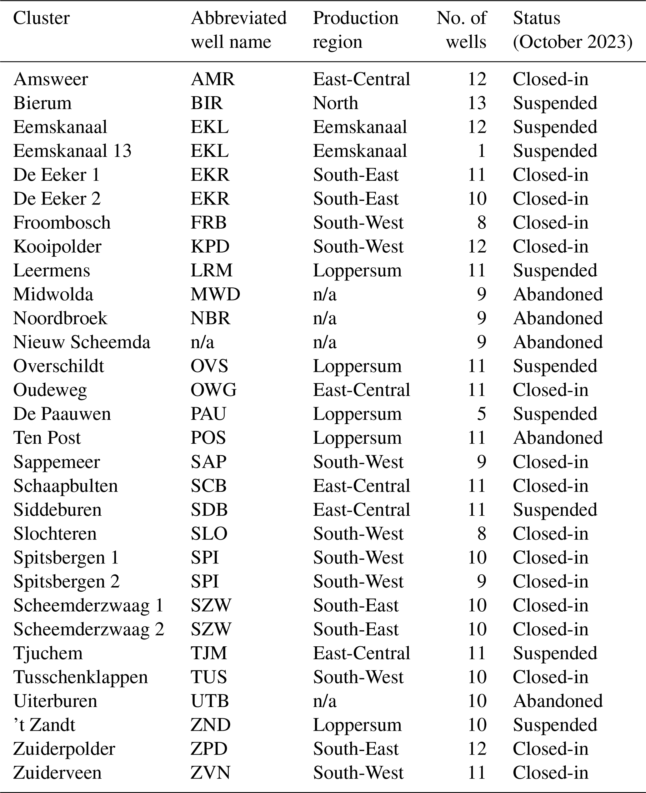
We consider a series of scenarios for gas injection with different spatial and temporal distributions of total gas volume injection rates. Available total volumes of N₂ for one set of scenarios are informed by the currently available N₂ generation capacity in the Netherlands. The spatial distribution of gas injection for all scenarios is based on the location of available wells in the Groningen field at the time of end of production (end of 2023). The 335 Groningen gas wells are grouped into clusters and production regions that are listed in Table A2 in Appendix A and shown in Fig. 2. For simplicity we assume that all gas production from nearby small fields that are included in the model ends on 1 October 2023 and that both the small field wells and pseudo aquifer wells implemented in the model are shut in at that time. The status of production well clusters in the field is explained in Table A2.

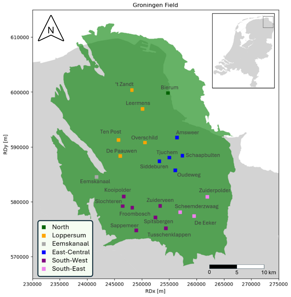
Figure 2 Overview of gas well clusters and past production regions in the Groningen field. The status of wells in these clusters is summarized in Table A2 in Appendix A.

Table A2 also indicates the status of the well clusters just before closure of the field. We assume that both closed-in and suspended wells can be made available for injection while abandoned wells cannot be reused. Throughout, we will assume that N₂ is available to be injected at all wells that are potentially operational in the field. That is, the availability and/or suitability of the surface infrastructure and the sourcing and distribution of the N₂ are not explicitly considered and studied.

Scenarios are defined in terms of the distribution of a total volume rate over all available wells in one or more production regions. The distribution of the total volume injection rate over all individual wells is calculated by the simulator based on the injection potential of each well, with a maximum set by its historic production rate. In the following we discuss the various scenarios in detail.

In the “no injection” base case (reference) scenario, no gas is injected. Gas flow will still occur, however, due to the existing pressure gradients in the field that result from uneven gas production in the past. This scenario provides the baseline expectation for seismicity.

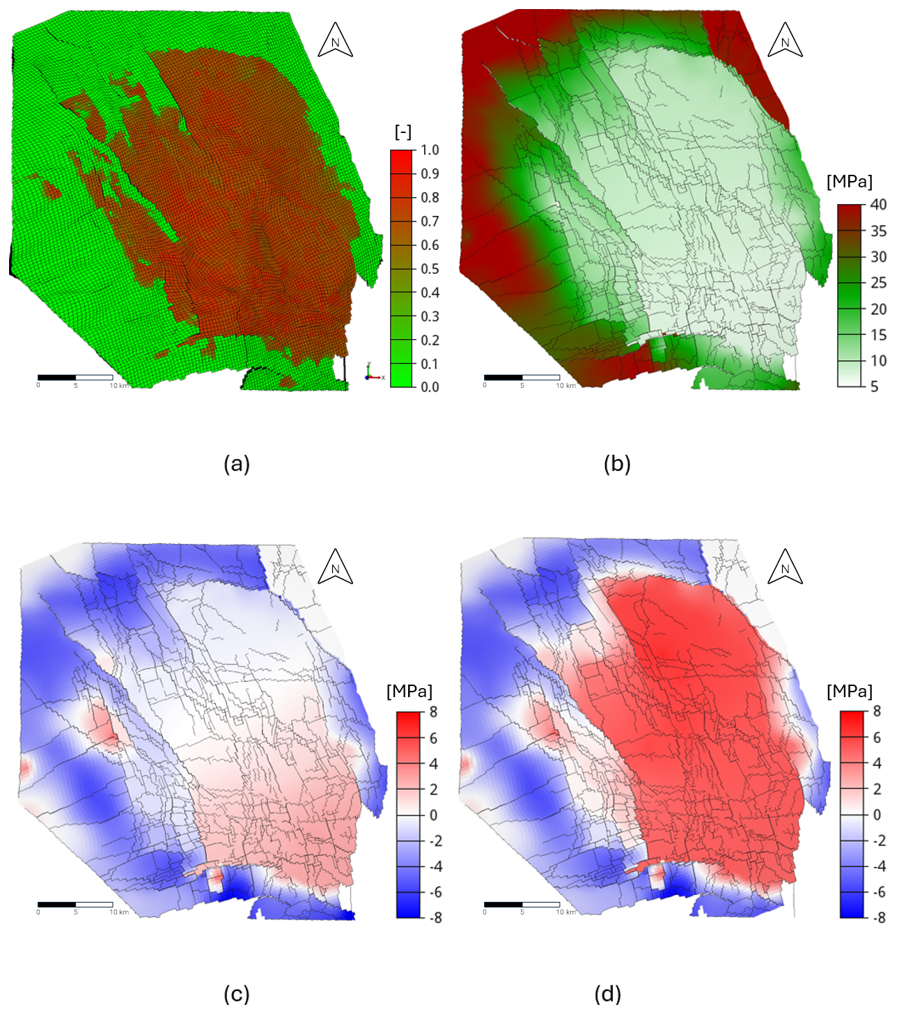
Figure 3 (a) Top view of the initial gas saturation [–] on the simulation grid. (b) Pressure [MPa] at the end of production (October 2023). (c) Change in pressure [MPa] over the injection period for the SE scenario. (d) Change in pressure [MPa] over the injection period for the LO_SE-10ZB scenario.

One set of scenarios involves gas injection in the Loppersum area, which has experienced the highest seismic activity, including the largest event registered to date (M 3.6), at Huizinge. While production from this area was stopped in 2018, production continued from the south of the field. This has resulted in a pressure gradient towards the south-east of the field (see Fig. 3) which will lead to flow of gas away from the Loppersum region, and therefore to local lowering of the pressure and associated compaction of the reservoir. Injection in this area could potentially deliver direct beneficial effects on seismicity by, at least temporarily, maintaining pressure. At the same time, this would maintain or even strengthen the existing large-scale pressure gradient and thus cause gas to flow away from the injection area. Retaining any positive impacts would therefore require sustained injection over a long period until large-scale pressure equilibration has been established. As soon as injection is stopped, local pressure may be expected to start to decline again, but possibly at a slower pace than before.

The south-east region of the field has depleted most strongly (i.e. pressure is lowest here), since gas production during the most recent years up to cessation of operations has primarily occurred here, and therefore will be a driver for redistributive large-scale flow in the field. An increase in pressure in this region should reduce the large-scale pressure gradient across the field and thus permanently reduce the trend towards further pressure decline in regions further north. However, beneficial effects on seismicity in the Loppersum area can be expected to occur slower and later than if gas were actually injected there. A compromise scenario that could deliver both short-term direct benefits, as well as slower, but long-term, ones, is therefore to inject in both the Loppersum and South-East regions.

The total availability of injection gas used in the scenarios will be based on assumptions about the capacity of factories for N₂ generation. One of these facilities is the recently completed phase II extension of the Zuidbroek factory, which has a reported capacity of 180 000 m³ h⁻¹ (Gasunie, 2025). For brevity we will refer to the Zuidbroek phase II capacity as 1 ZB, i.e. 1 ZB = 180 000 m³ h⁻¹ (or, equivalently 1.58 × 10⁹ m³ yr⁻¹, where 10⁹ m³ = 1 billion cubic meters = 1 BCM). The first set of scenarios that we consider assumes a continuous N₂ generation capacity of 1 ZB. This is based on a rough estimate of the spare capacity of all combined N₂ generation facilities in the country, which includes the full Zuidbroek facility (the total capacity is estimated to be roughly 3.2 ZB or 5.1 BCM yr⁻¹). With spare capacity we mean the capacity not immediately needed to meet the current requirements for conversion of high-caloric imported gas to Groningen-grade gas. For the year 2023 Gasunie Transport Services (GST) reported using 2.84 BCM of N₂. This would suggest a spare capacity of about 2.2 BCM yr⁻¹, or 1.4 ZB. We will consider the scenario that 1 ZB of this capacity is available for continuous injection throughout the year. We stress that the actual value is uncertain and may be lower.

Table 1 Overview of injection scenarios. All injection scenarios are simulated until 2054. Injection is started in October 2025 in all cases except scenario 1. Volume factors express the total injected surface volume rate in terms of the of Zuidbroek Phase II extension N₂ production capacity (180 000 m³ h⁻¹). The time to stop injection in scenario 8 (9) is based on the results from scenario 5 (6) and corresponds to the time that model-predicted seismicity is reduced to zero.

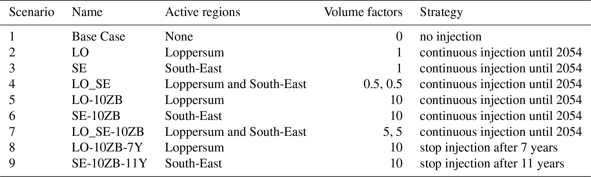
It is possible that scenarios that consider a relatively modest N₂ generation capacity of 1 ZB will not lead to very significant reduction of seismicity in the short term. We will therefore also consider a set of scenarios that assume a N₂ injection capacity of 10 ZB. These more scientifically motivated scenarios are expected to help understand and illustrate fundamental mechanisms associated with re-pressurization and its impact on seismicity. The complete set of scenarios considered in this study is summarized in Table 1. Scenarios LO, SE, and LO_SE are based on a total N₂ generation and injection capacity of 1 ZB, while scenarios LO-10ZB, SE-10ZB, and LO_SE-10ZB are the corresponding scenarios for a capacity of 10 ZB. Scenarios LO-10ZB-7Y and SE-10ZB-11Y are informed by results obtained for scenarios LO-10ZB and SE-10ZB and are meant to investigate the hypothesis of re-bouncing of seismicity due to pressure equilibration throughout the field after cessation of injection. To that end, in scenarios LO-10ZB-7Y and SE-10ZB-11Y, injection is stopped at the time that model-predicted seismicity rate is less than 1 event per year in scenarios LO-10ZB and SE-10ZB respectively. As an explanation of the volume factors listed in Table A2, consider e.g. scenario LO_SE. The total injected rate corresponds to 1 ZB, and this volume is divided equally over the Loppersum and South-East regions. So 0.5 ZB is injected in Loppersum and 0.5 ZB is injected in the South-East region.

4 Results

4.1 Pressure

The initial gas saturation and the field pressure at the end of the production period are shown in Fig. 3a and b, while changes in pressure over the injection period for two scenarios are shown in Fig. 3c and d. The initial pressure at the top of the reservoir was approximately 34.5 MPa. The largest simulated changes in pressure over the production period (25–28 MPa) are observed in the gas zone, with some dissipation into the surrounding aquifers. The pressure state at the end of production in October 2023 is the starting point for simulations over the forecast period 2024–2054. In our simulations we assume that injection is started in October 2025, following a 2-year shut-in period. Maximum increases in reservoir pressure as a result of gas injection of about 2.5 and 7.0 MPa respectively can be observed for the scenarios SE and LO-10ZB. Figure 4 shows simulated near-well pressures over the injection period for all scenarios at the locations of 4 inactive wells. Pressure curves are provided for the Amsweer 1, Eemskanaal 1, Ten Post 1, and Spitsbergen 1 wells, which are located in the Central-East, Eemskanaal, Loppersum and South-West production regions respectively. All four wells are inactive during the forecast (injection) period. For the wells Eemskanaal 1 and Ten Post 1, located in the Eemskanaal and Loppersum regions respectively, the pressure tends to decline if no gas is injected due to pressure equilibration (see the black lines). Since pressure in these regions is initially higher than in the regions towards the east and south, the resulting pressure gradient will drive a gas flow that would ultimately result in a more or less homogeneous pressure throughout the field. At the Eemskanaal cluster location this tendency is observed for the first 6 to 20 years also when gas is injected in the Loppersum or South-East regions. The pressure decline stops earlier and at a higher value when the total injected volume is higher (compare e.g. the 1 ZB and 10 ZB injection scenarios for the Eemskanaal 1 location).

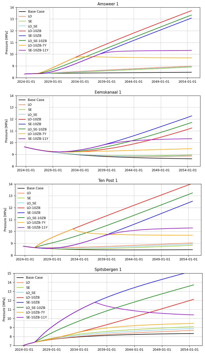
Figure 4 Simulated near-well average reservoir pressure [MPa] around 4 wells from 4 different production regions: Amsweer 1, located in the East-Central region, Eemskanaal 1, located in the Eemskanal region, Ten Post 1, located in the Loppersum region, and Spitsbergen 1, located in the South-West region. Results are shown for all scenarios. The wells are not used for injection.

As expected, the pressure increases much faster when gas is injected with a higher volume rate. Considering, for example, the location of the Amsweer 1 well, pressure is increased by up to 0.6 MPa over the 30 year injection period for an injection rate of 1 ZB, while an increase up to 5 MPa is observed over that same period for a rate of 10 ZB. For context, these values compare to a historical pressure decline at this location of about 26.2 MPa over the production period. Since this well is somewhat closer to the Loppersum region than to the South-East region, the pressure increase is somewhat delayed if the gas is injected in the South-East region (compare e.g. the blue and yellow lines). At the Ten Post 1 well location interesting behaviour is observed for scenario LO-10ZB-7Y, yellow line). Pressure decreases during the first few years after the end of production and before the start of injection. Pressure builds up quickly for a period of 7 years when large volumes of gas are injected using wells in the same production region. When the injection is stopped after 7 years pressure starts to decline again immediately, reaching its lowest value at the end of the forecast period in 2054. If gas is injected in the South-East region (scenario SE-10ZB-11Y, the purple line), the initial pressure decline takes somewhat longer to reverse, but no second period of pressure decline is observed in this case, also not after 11 years, when injection is stopped.

Similar behaviour can be observed at the Spitsbergen 1 well location. This location is fairly close to the South-East production region and a clear decline of pressure is observed when injection is stopped after 11 years SE-10ZB-11Y. No initial decrease in pressure is expected at this location due to the fact that pressure is already very low in the south of the field at the end of production. Gas will therefore tend to flow towards this location, especially from further north where the pressure is higher, even in the case that no gas is injected.

4.2 Temperature

The reservoir temperature at the end of the injection period for the injection scenario LO-10ZB is shown in Fig. 5. Temperature changes are observed around the 4 active clusters in the Loppersum region, and at a water injection site in the east of the field. Maximum cooling by just over 52 °C is observed, which compares to an initial temperature of around 102 °C. Significant cooling is limited, however, to the cells that are intersected by the injection wells, with some minor cooling of directly neighbouring cells (note that the average grid cell width is close to 400 m).

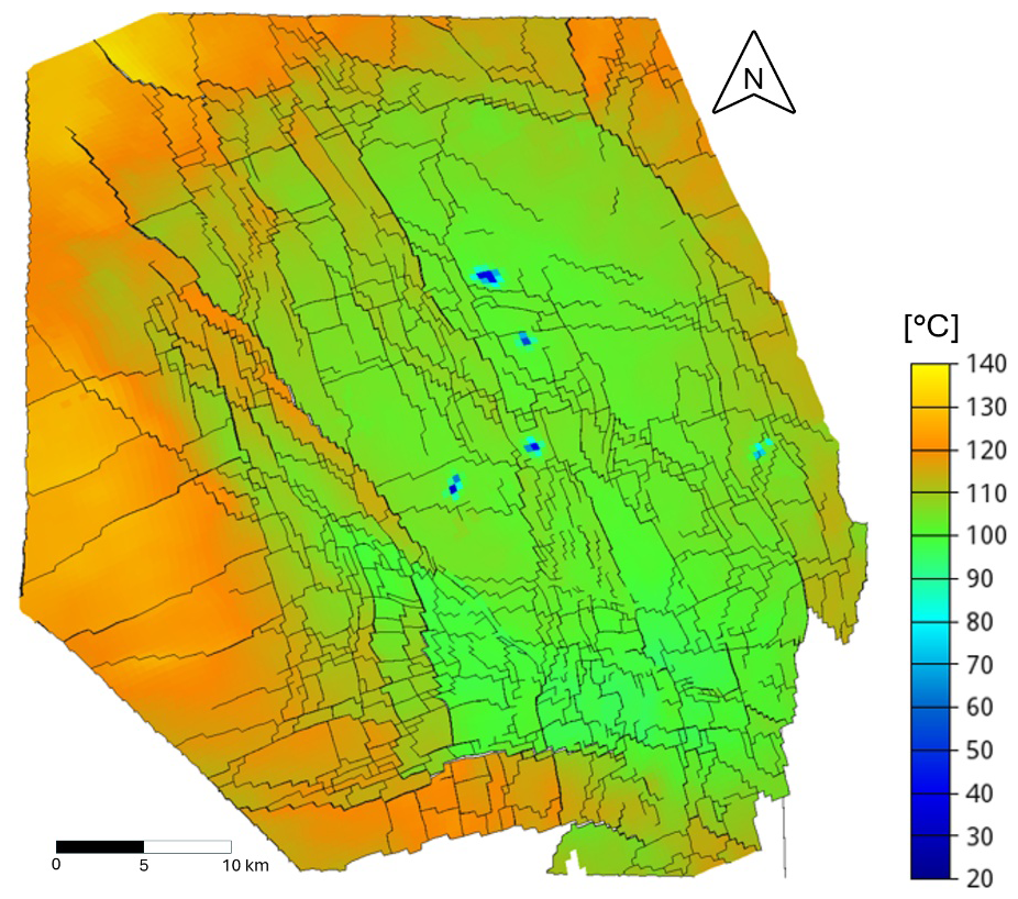
Figure 5 Temperature [°C] at mid-reservoir depth (Upper Slochteren formation) in 2054 for injection scenario LO-10ZB, for an injection temperature of 10 °C.

4.3 Seismicity

The seismic source model parameters (see TNO 2020, for a complete overview) are calibrated on the past seismicity with M_min = 1.45 over the period 1 January 1995–28 February 2023. This calibration is performed simultaneously for the spatial domain, temporal domain and magnitude domain. The resulting calibrated model result (the posterior predictive rate, giving the hindcast over the calibration period) is compared to the calibration data in Fig. 6, and shows a good match in the magnitude, temporal, and spatial domain. While the comparison in Fig. 6 is based on marginal distributions (sums over all dimensions except those of interest) for visual comparison purposes, the calibration is performed by comparing the full space-time-magnitude model outcomes against the observations. The applicability of these calibrated parameters to future scenarios is grounded in the assumption that the fundamental physical relationships, specifically the sensitivity of seismic activity to pressure and temperature changes, remain stationary over time. By capturing these underlying mechanics during the historical period, the model parameters capture the intrinsic response of the reservoir, ensuring that the forecasts remain physically consistent even as operational conditions evolve. For the historic period, the modelled pressure and temperature changes are identical for all scenarios. The pressure changes are based on history matching, while the temperature changes are only modelled in a forward sense. Even though the temperature changes over the historic period are modest, the Bayesian inference procedure used for calibration results in a posterior distribution for the a_T parameter which is noticeably distinct from the prior distribution, indicating that there is significant information about this parameter contained in the data (see Fig. A1 in Appendix A).

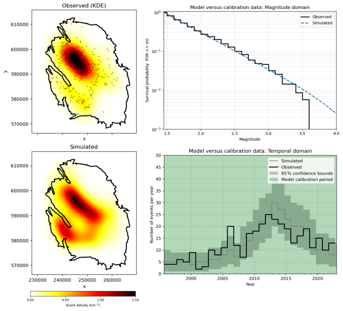
Figure 6 A comparison between the calibrated model and the calibration data. On the left side of the figure: the observed spatial distribution of events (top) vs. the modelled spatial distribution. On the top right side of the figure: the observed magnitude distribution vs. the modelled magnitude distribution. On the bottom right side of the figure: the observed temporal distribution vs. the modelled temporal distribution.

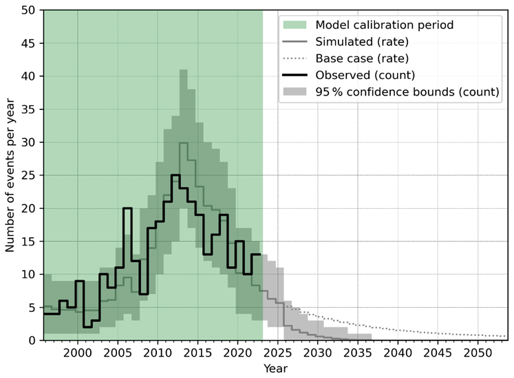
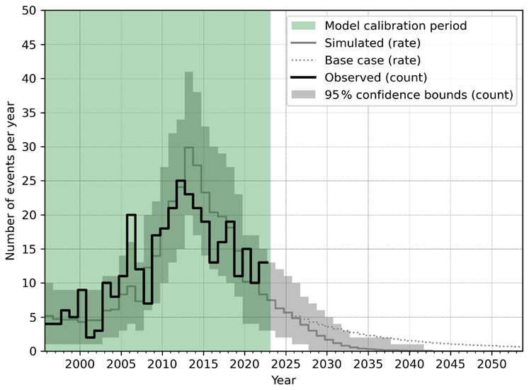
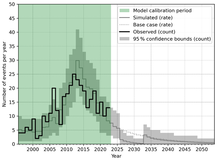
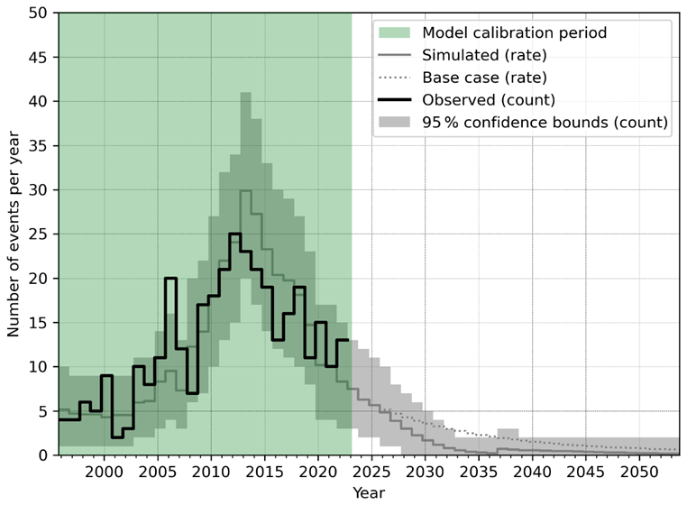
For all scenarios detailed in Table 1, we forecast the event rate until October 2053, and provide a full seismicity forecast (including magnitudes, suitable for hazard and risk assessment) for the years 2024 until 2037. Since this study focusses on the difference in impact of different N₂ injection scenarios, which are most clearly visible in the first 13 years of these scenarios, full seismicity forecasts, as well as hazard and risk calculations beyond 2037 are not provided. We present a selection of results here to support our main findings. Specifically, Figs. 7 to 14 show seismicity profiles for all scenarios. In the seismicity profiles (showing the number of events per year), the “reference” refers to the scenario with no injection. Figures 7 to 14 are based on the model settings in which temperature effects are included. Figures for the same scenarios, but without the temperature effect, are included in Appendix A (Figs. A2 to A9).

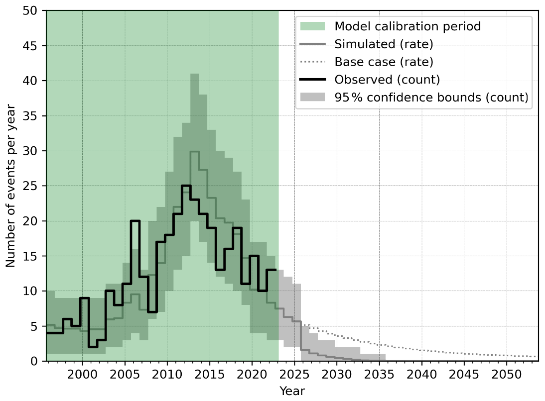
Figure 7 Number of events per year in the Groningen field of magnitude M 1.5 and above for the LO-10ZB scenario (with temperature effects included). The solid grey line is the modelled expected number of events, the grey area gives the 95 % confidence bounds per year. The solid black line is the historically observed event rate and the green area is the period over which the model is calibrated. The dotted reference line represents the base case for comparison.

Figure 8 As Fig. 7, except for the LO scenario.

Figure 9 As Fig. 7, except for the LO_SE scenario.

Figure 10 As Fig. 7, except for the SE scenario.

Figure 11 As Fig. 7, except for the LO_SE-10ZB scenario.

Figure 12 As Fig. 7, except for the SE-10ZB scenario.

Figure 13 As Fig. 7, except for the LO-10ZB-7Y scenario.

Figure 14 As Fig. 7, except for the SE-10ZB-11Y scenario.

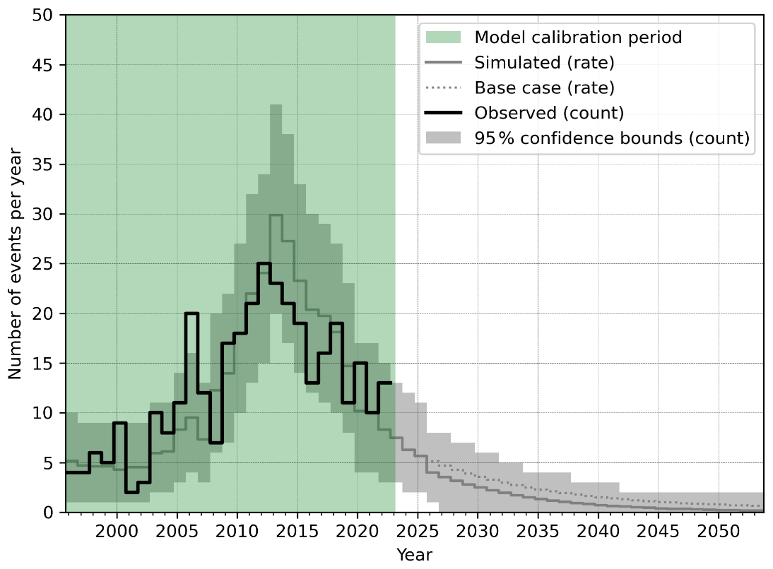
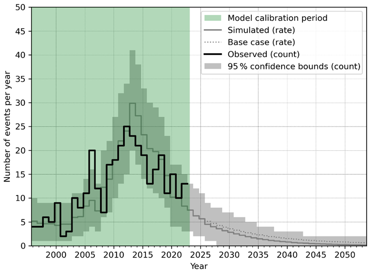
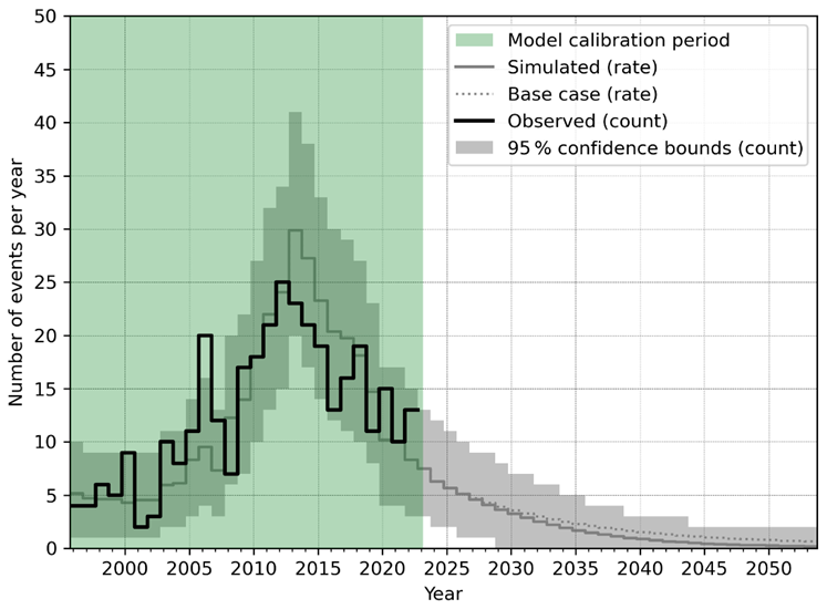
For all scenarios, we perform the forecasting by integration over the full posterior model parameter space to obtain the posterior predictive forecast. We consider two model choices in more detail. For the first choice, the seismic source model only accounts for the pressure changes and does not account for temperature changes. This conforms to the original source model, excluding the modification to account for temperature effects, and is also identical to the Maximum Likelihood Estimate for the temperature influence parameter (a_T=0.) For the second choice, we do use the modification where temperature changes lead to additional strain, and more specifically, where cooling leads to additional seismicity. To include this effect, we integrate over the full posterior model parameter distribution, including a_T.

The main effects that can be seen are as follows. Injecting more N₂ leads to a faster reduction of seismicity in the forecasts (from comparison with the dotted line for the no-injection reference). In the 10 ZB (high injection volume) scenarios, seismicity rapidly declines to zero expected events per year in 7 to 11 years, depending on the injection location (Figs. 7, 11, 12). In contrast, in scenarios where the equivalent of one-tenth of that volume is injected (1 ZB), the decline in seismicity is slower and reaches close to zero expected events after approximately 25 years of continuous injection (Figs. 8, 9, 10).

When considering the same injection volume, injecting in the Loppersum area leads to a faster reduction in seismicity compared to injecting the South-East. The seismicity reduction for injection of equal volumes in the Loppersum and South-East areas (cases LO_SE and LO_SE-10ZB) falls in between these two end-members.

Although injection in the Loppersum area leads to a faster decline in seismicity compared to other tested spatial N₂ distribution scenarios, it is also associated with the largest increase in seismicity after injection stops (Fig. 13). This is due to the pressure equilibration in the field that will continue after cessation of the injection. Injection in the Loppersum area maintains the spatial pressure differences in the field, which then leads to gas flow to equilibrate pressures.

In the models, the role of temperature changes is very limited. The seismicity rate for the scenarios with and without temperature effects on seismicity are nearly identical (within 1 %). This is due to two main factors:

1. The calibration on the (limited) past temperature changes assigns most posterior probability to model parameters corresponding to little to no effect of temperature on seismicity.

2. Anywhere in the model where the temperature decreases due to injection, the pore pressure goes up due to that same injection. In fact, the pore pressure goes up enough to completely undo any shrinkage caused by the cooling. Consequently, in these parts of the model, there is zero seismicity forecasted, despite the temperature decrease.

This leads to the slightly counter-intuitive result that including the adverse effects of cooling into the model leads to (marginally) lower seismicity rates. This result stems from the fact that if cooling is modelled to cause seismicity, then some of the past seismicity should be “attributed” to cooling, rather than to pore pressure changes. In other words, pore pressure changes are calibrated to be slightly less effective at causing seismicity if we assume that cooling can be partially responsible for past and future seismicity.

In any given forecast, the cooling always fully falls within the zone where no seismicity is modelled due to the local pore pressure increasing significantly. Therefore, cooling does not end up causing any seismicity in the forecasts. For any given scenario, the modelled pore pressures are identical, regardless of whether cooling is assumed to cause seismic activity. However, as explained above, if we assume that cooling can contribute to seismicity, the same pore pressure decrease leads to slightly less seismicity.

It is important to emphasize that the differences in seismicity rate are extremely small, and can effectively be considered to be identical.

4.4 Seismic hazard and risk

Figures 15, 16, and 17 show the hazard maps (PGA for a 475 year return period) for the reference case, the LO case and the LO-10ZB case. The general pattern of hazard is comparable to that of the seismicity maps (not shown here). The hazard is higher in areas with more expected earthquakes. The hazard maps also show the effects of the shallow subsurface (through the site response model in the Ground Motion Model), which can locally amplify ground motions and therefore increase the hazard, depending on the mechanical properties of the shallow subsurface layers.

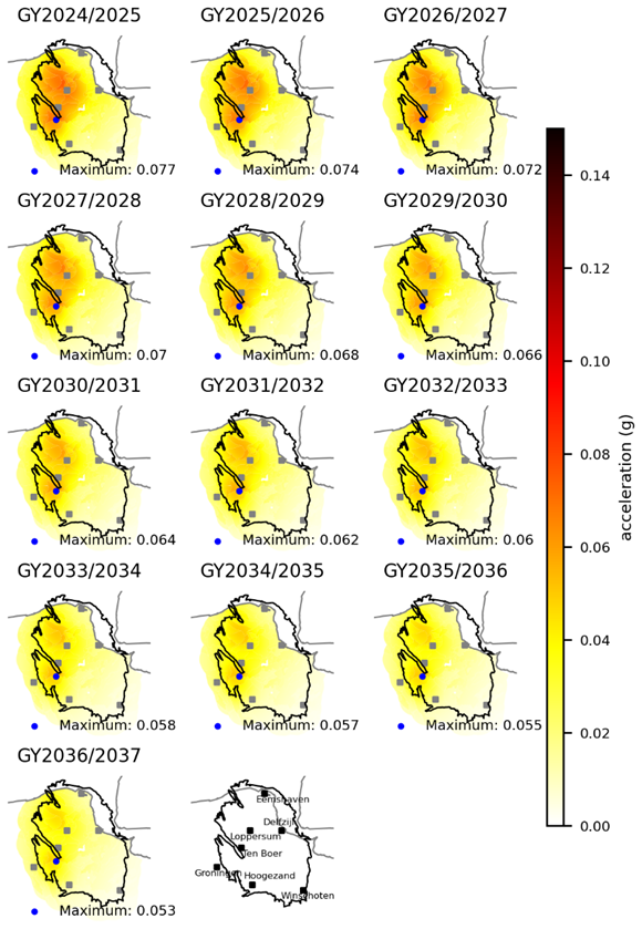
Figure 15 Peak Ground Acceleration (pseudo-spectral acceleration at 0.01 s) hazard map for a 475 return period (10 % probability of exceedance in 50 years). The blue dot indicates the position of the largest hazard for each year. Base case (no injection).

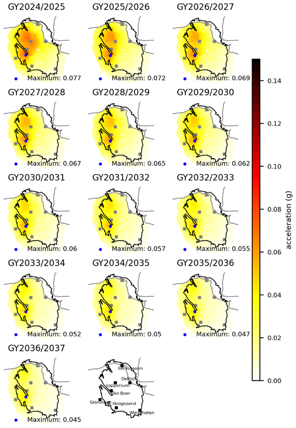
Figure 16 As Fig. 15, but for the LO scenario.

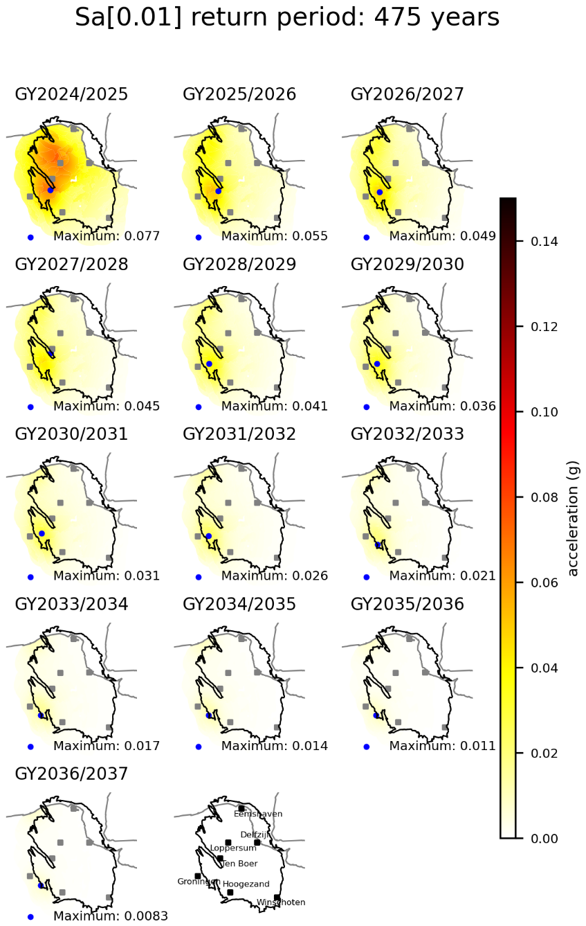
Figure 17 As Fig. 15, but for the LO-10ZB scenario.

Figure 18 shows the risk exceedance curves for selected years up to 2036/2037. As is typical in the context of Groningen seismicity, risk is expressed in terms of “Local Personal Risk” (LPR) which is the annual probability of fatality due to (partial) structural collapse of the building caused by an induced earthquake. The LPR is calculated on a per-building basis, under the assumption that one person is continuously present in or around the building. Since injection for all cases except the base (reference) case starts on 1 October 2025 (the first day of gas year 2025/2026), the risk is identical for all scenarios in gas year 2024/2025 (Fig. 18a). Over the subsequent years, we see a general reduction in the risk for all scenarios when compared to the base case. When gas is injected in the Loppersum area at a rate equivalent to the Zuidbroek II production capacity (1 ZB), the number of buildings that do not conform to the safety norm (LPR of 10⁻⁵ yr⁻¹ (Commisie Meijdam, 2015)) goes from ∼ 500 to ∼ 200 after 1 year of injection (Fig. 18b). The most pronounced reduction occurs when 10ZB is injected in the same area, resulting in a reduction to ∼ 3 buildings after only 1 year. However, if injection in this scenario is stopped after 7 years (when the expected fieldwide event rate is less than one under the continuous injection scenario), the number of buildings that don't conform to the safety norm goes back up to ∼ 300 (Fig. 18c), due to the reappearance of seismicity associated with pressure redistribution in the gas reservoir. If the same volume of gas is modelled to be injected in the South-East clusters, the decline of seismic risk is less rapid. However, the increase in risk level associated with cessation of the gas injection is much less pronounced (Fig. 18d). In other words, injection scenarios that (partially) inject the N₂ in the South-East clusters have less pronounced effects on seismicity, hazard, and risk on the short term, but potentially offer advantages on the longer term, since they reduce spatial gas pressure variability, and therefore are associated with less pressure equilibration once gas injection eventually ceases.

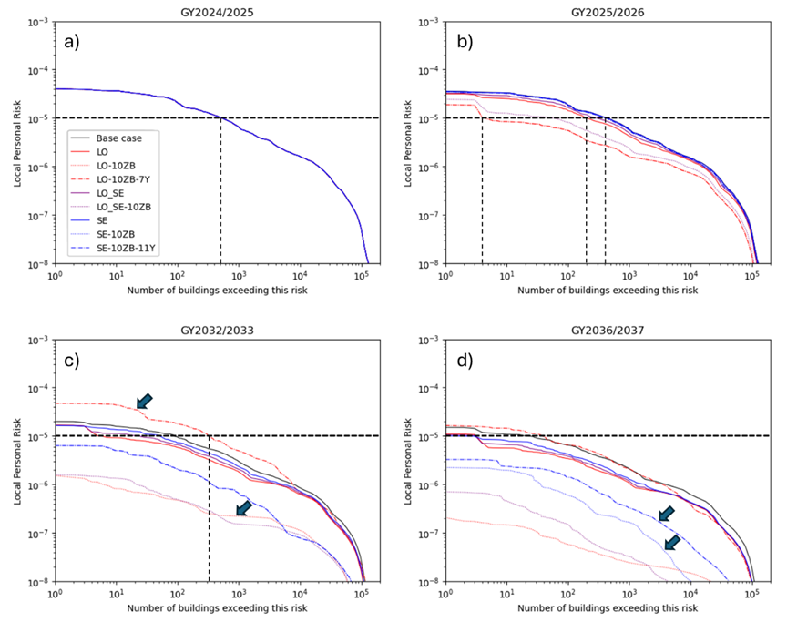
Figure 18 Risk exposure plots, showing how many buildings (on the x-axis) are exposed to a given local personal risk (y-axis). Shows all scenarios considered for gas years 2024/2025, 2052/2026, 2032/2033 and 2036/2037. Approximately 500 buildings exceed the Meijdam norm (10⁻⁵ yr⁻¹) for all scenarios for gas year 2024/2025. The dotted vertical lines are shown to indicate the origin of number of buildings quoted in the text. The arrows in panels (c) and (d) point to scenarios that are identical, with the exception of stopping injection after 7 or 11 years.

Whether or not cooling effects are included in the seismicity forecasts hardly affects the resulting risk profiles. Our results show that the difference in risk is almost entirely determined by the choice of injection scenario, rather than by whether or not cooling-induced seismicity is included in the source model or not (see Appendix A Fig. A10).

5 Discussion

Several assumptions and simplifications had to be made in this study. We comment on these here and provide arguments for their possible relevance and impact on the presented results.

We have considered relatively simple scenarios for gas injection where we have assumed constant N₂ generation and injection capacity. Future changes in available injection capacity related to changes in overall gas production and usage, or even the addition of an additional N₂ facility, could be imagined. Given the low pressures currently present in the field, and the relatively low-volume injection rates that we consider here in the 1 ZB scenarios, pressure increases will approximately scale linearly with the average volume injected for pressures up to 2000 psi (see e.g. the last parts of the curves in Fig. 4 after transient effects have more or less disappeared). This means that, given an average injection rate of e.g. 2 ZB, pressure increases relative to the no injection case can be expected to be higher by approximately a factor 2 than the pressure increase obtained for an average injection rate of 1 ZB.

We have assumed that individual wells cannot inject at rates higher than their maximum historic gas production rates. These maximum production rates range from 0.2 to 1.2 ZB for wells in the Loppersum region, and from 0.1 to 0.7 ZB for the wells in the South-East region. This means that the wells with the highest productivity (> 1 ZB) could already by themselves inject all N₂ injected in the LO scenarios. In our model simulations nearly 60 wells were used for the scenarios where gas is injected in the South-East region. The high well productivity estimates imply that this number of wells could in principle be strongly reduced.

The effectiveness of gas injection may depend on the composition of the injected gas. In our model simulations we have assumed injection of “Groningen gas”, i.e. gas with the same composition as the gas already present in the reservoir. The effect of gas composition was investigated separately with the use of a compositional simulator where we compared the pressure evolution for injection of identical surface volumes of Groningen gas and N₂ in the same closed volume. These simulations suggest that injection of N₂ will result in a faster increase in pressure by a factor of 1.14 after 30 years of injection. This implies that the presented results could be interpreted as a lower bound on expected pressure effects, or an upper bound on the volumes of gas required to reach a desired pressure state.

It is important to note that the seismic source model used in this study was developed with gas production in mind, and was calibrated on seismicity generated by gas production, when no gas injection and very limited water injection was taking place. As a result, the results obtained for different injection scenarios are automatically less well constrained. The source model may not include all physical mechanisms that are relevant in an injection scenario. For example, in the current implementation of the seismic source model, any local gas pressure decrease leads to seismicity, even if that particular location has seen even lower gas pressures in the past (i.e. we assume that the Kaiser effect (Kaiser, 1953) does not play a role). Furthermore, we've implemented our temperature-dependent seismic source model on the basis of linear thermo-elasticity. This ignores the role of time-dependent compaction, which is expected to play a role in Groningen (Aben et al., 2025; Pijnenburg et al., 2019). In the source model, total compaction (vertical strain) at offset faults drives the seismicity. On the short term, the time-dependent component of the compaction may continue to contribute to seismicity, making N₂ injection less effective at mitigating seismicity than it would be in a purely elastic reservoir. However, it is important to note that this effect is expected to be limited in both space and time, and that N₂ injection is expected to contribute to an earlier end of seismic activity, even when considering time-dependent compaction of the reservoir.

Nonetheless, these results give us first order indications on the effects of different quantities of N₂ injection, and the effects of the spatial distribution of that injection. In particular, they suggest that the potential positive effects of large-scale N₂ injection on both seismicity rate (the number of earthquakes per unit time) and seismic risk (the probability of loss of life due to seismicity) can be substantial compared to the “no injection” base case.

The variability of seismic hazard and risk results between scenarios with the same amount of injected gas shows that there is room for optimization of spatial and temporal distribution of gas injection over the available wells. Further exploring this aspect is outside the scope of this work. We have also not explored how a long-term injection strategy could be developed that includes eventually ending the N₂ injection. Such an “exit-strategy” is clearly needed, as infinite injection in unfeasible from many perspectives, including physical considerations.

We stress that the scenarios explored in this study are hypothetical. Practical feasibility of specific injection scenarios would depend on aspects that have not been fully considered, such as the costs of N₂ generation, the possibility to re-use existing infrastructure, including wells and transport pipes, societal support, etc.

While the modelling approach used here was developed specifically for the Groningen case, it could in principle also be applied to other gas fields. Furthermore, while we have focussed on scenarios for gas injection after cessation of production from the field, the methodology could be applied also to study the effects on seismicity of pressure maintenance during production.

6 Conclusions

We have investigated the potential effects of N₂ injection in the Groningen gas field on seismic event rate, seismic hazard, and seismic risk. To this end we have described the extension of the linearly elastic seismic source model. Rather than assuming a single value for the thermal expansion coefficient, we have explored the connection between the thermal expansion coefficient and the uniaxial compaction modulus to include the expected spatially heterogenous impact of temperature on strains throughout the gas field.

We looked at two total volume scenarios to get a sense for the general response to different amounts of N₂ injection, and different spatial distributions, all under the assumption that the only effect of injection is on the gas pressure and temperature distributions, and that locally increasing the gas pressure leads to less seismicity at that location, while locally decreasing temperatures lead to more seismicity.

The model experiments suggest that, if gas volumes similar to the capacity of the Zuidbroek II N₂ generation facility were available for large-scale injection, the positive effects on both seismicity rate (the number of earthquakes per unit time) and seismic risk (the probability of loss of life due to seismicity) could be substantial already after a single year of injection, when compared to the “no injection” base case. In one scenario, the number of buildings exposed to a risk level above the Meijdam norm is reduced from approximately 500 after 1 year without injection to approximately 200 after 1 year of gas injection. Without injection this reduction in risk level takes about 5 years. The effectiveness of injection depends on both the injection location and the total injected volume.

Appendix A

A1 Modelling parameters

Table A1 Modelling parameters used in the reservoir flow modelling.

A2 Well clusters and small fields

For simplicity we assume that all gas production from nearby small fields that are included in the model ends on 1 October 2023 and that both the small field wells and pseudo aquifer wells implemented in the model are shut in at that time. The status of production well clusters in the field is explained in Table A2.

Table A2 Status of well clusters in the Groningen field in October 2023 (End of Production). Note that the model also contains an additional number of pseudo aquifer wells to represent the effects of aquifers that are not explicitly modelled.

A3 Temperature effects on seismicity and seismic risk

In the main text of the manuscript we only show the seismicity and risk results using the “with temperature effects” model, since the effect of including/excluding temperature effects is very minor. For completeness, here we provide additional figures using the “without temperature effects” model. They only serve to further visually substantiate the claim in the main text that the effects are in fact very minor. This can be verified by comparing the seismicity rate Figs. A2 through A9 to the main text Figs. 7 through 14. For seismic risk, rather than showing even more nearly identical figures, we instead show the ratio of risk values on a per-building level in Fig. A10, which are very close to unity for all buildings, for all years, for all scenarios considered.

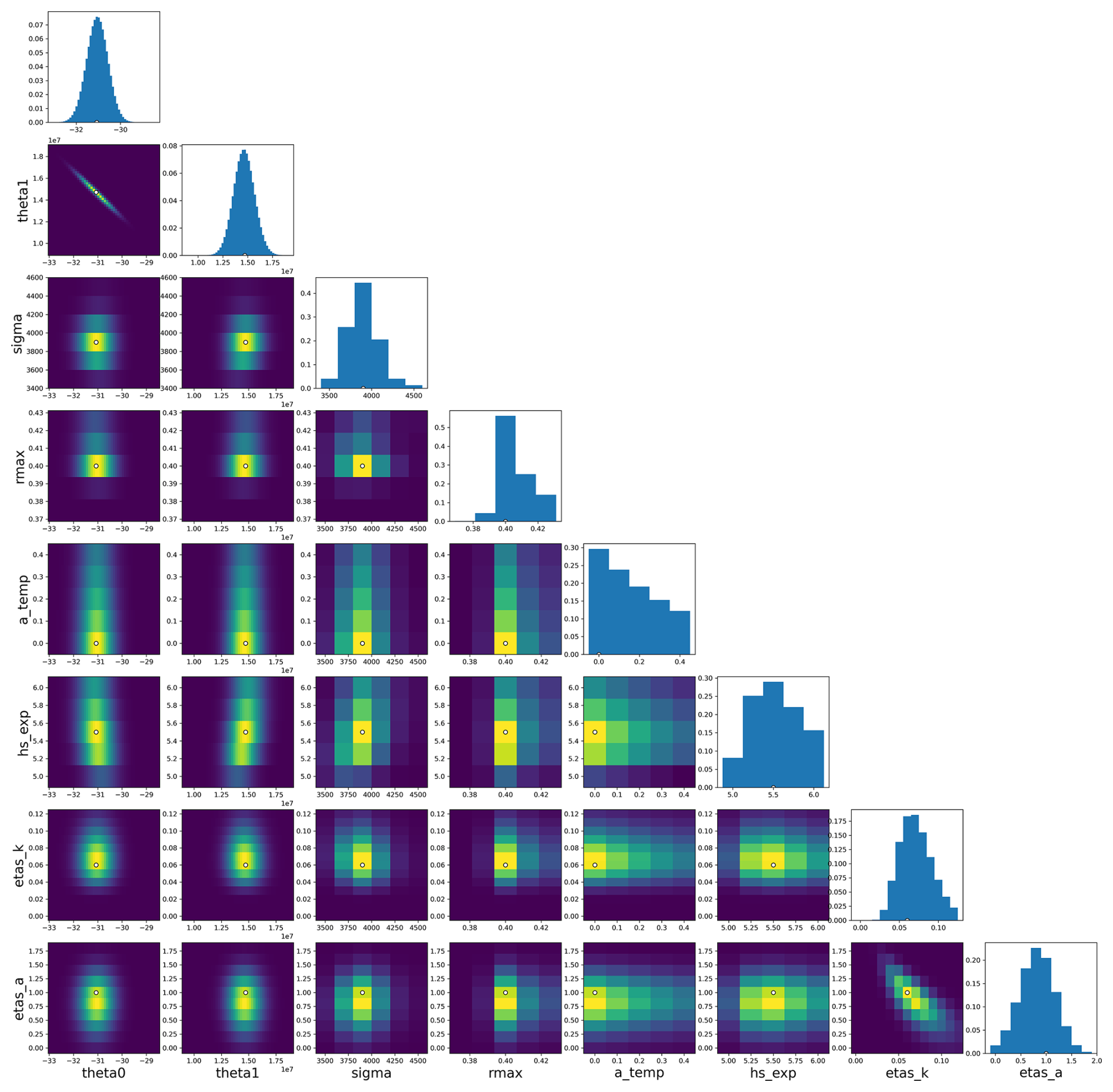
Figure A1 Posterior distribution of the model parameters for the earthquake rate model. See TNO 2020 for a complete overview. We calibrate the model on all observed earthquakes in the Groningen field with M_min = 1.45 over the period 1 January 1995–28 February 2023. The new parameter which relates to the impact of temperature changes on seismicity (a_T or a_temp in this figure) has been assigned a uniform prior probability over the range zero (no effect of temperature) to 0.4 MPa K⁻¹ (which corresponds to high sensitivity to temperature changes, α_T = 2.4 × 10⁻⁵ K⁻¹ for E = 15 GPa and ν = 0.2). The posterior distribution for a_T clearly shows a peak in probability density/mass at a_T = 0 and a rapidly decreasing probability density for higher values of a_T. This indicates that even based on the limited past temperature changes, the model performs better when these temperature changes do not result in seismicity.

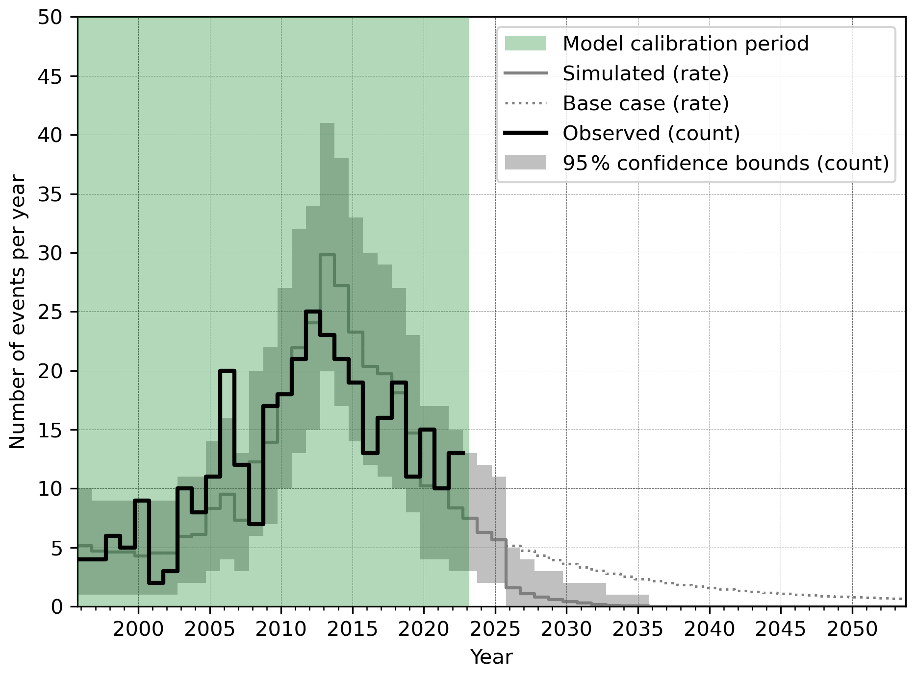
Figure A2 Number of events per year in the Groningen field of magnitude M 1.5 and above for the LO-10ZB scenario (without temperature effects included). The solid grey line is the modelled expected number of events, the grey area gives the 95 % confidence bounds per year. The solid black line is the historically observed event rate and the green area is the period over which the model is calibrated. The dotted reference line represents the base case for comparison.

Figure A3 As Fig. A2 except for the LO scenario.

Figure A4 As Fig. A2 except for the LO_SE scenario.

Figure A5 As Fig. A2 except for the SE scenario.

Figure A6 As Fig. A2 except for the LO_SE-10ZB scenario.

Figure A7 As Fig. A2 except for the SE-10ZB scenario.

Figure A8 As Fig. A2 except for the LO-10ZB-7Y scenario.

Figure A9 As Fig. A2 except for the SE-10ZB-11Y scenario.

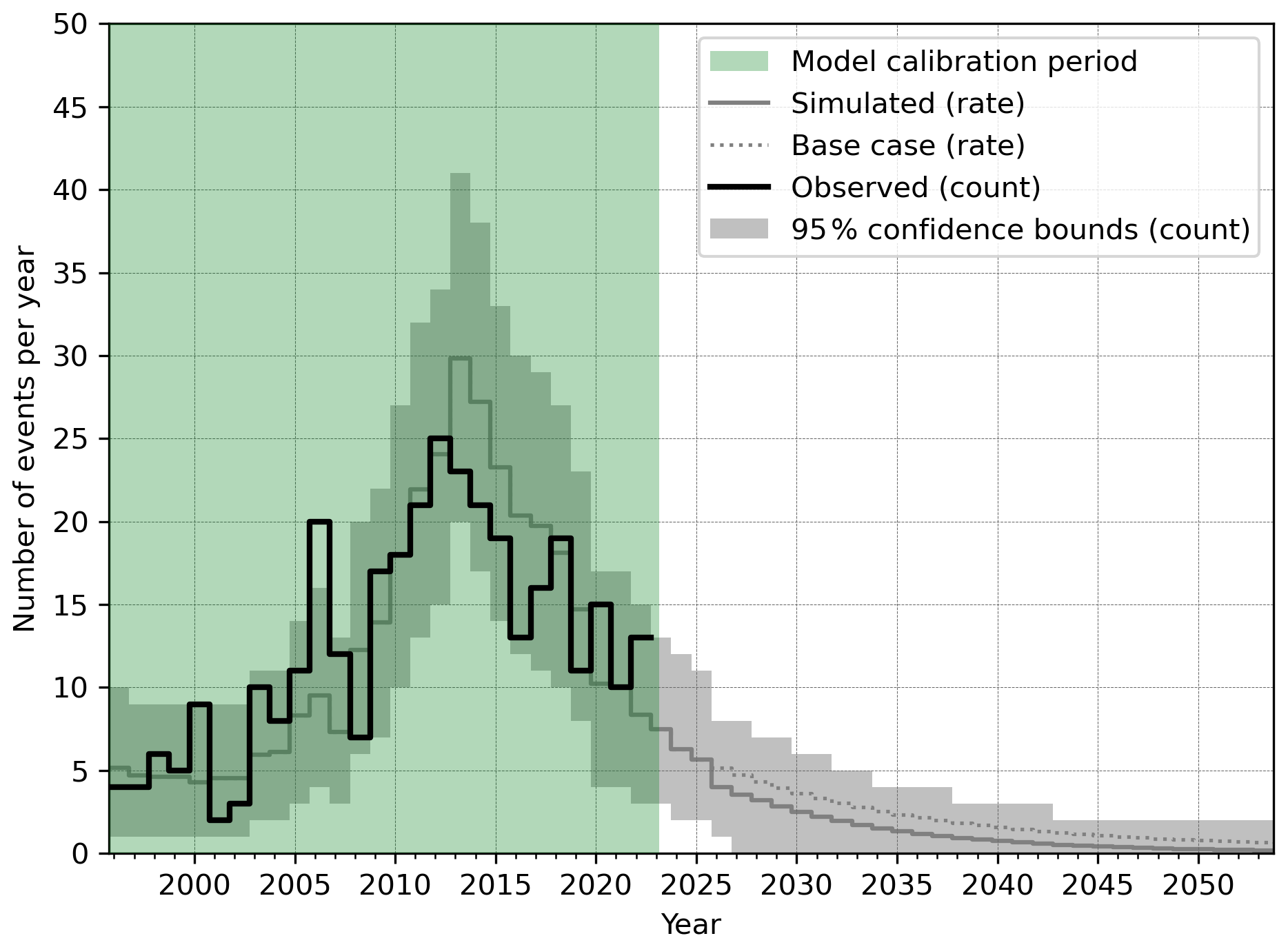
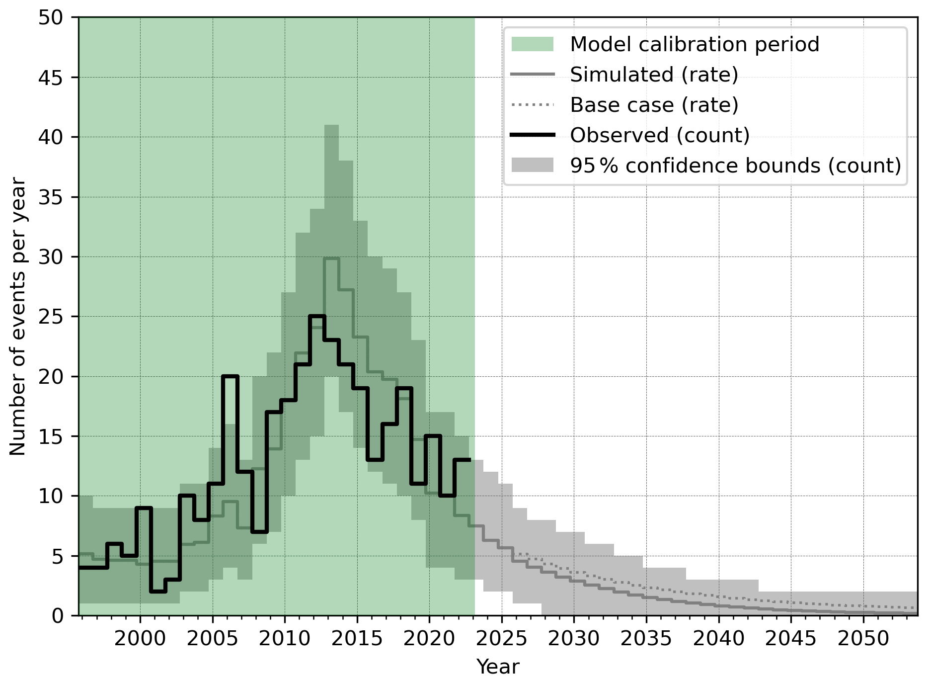
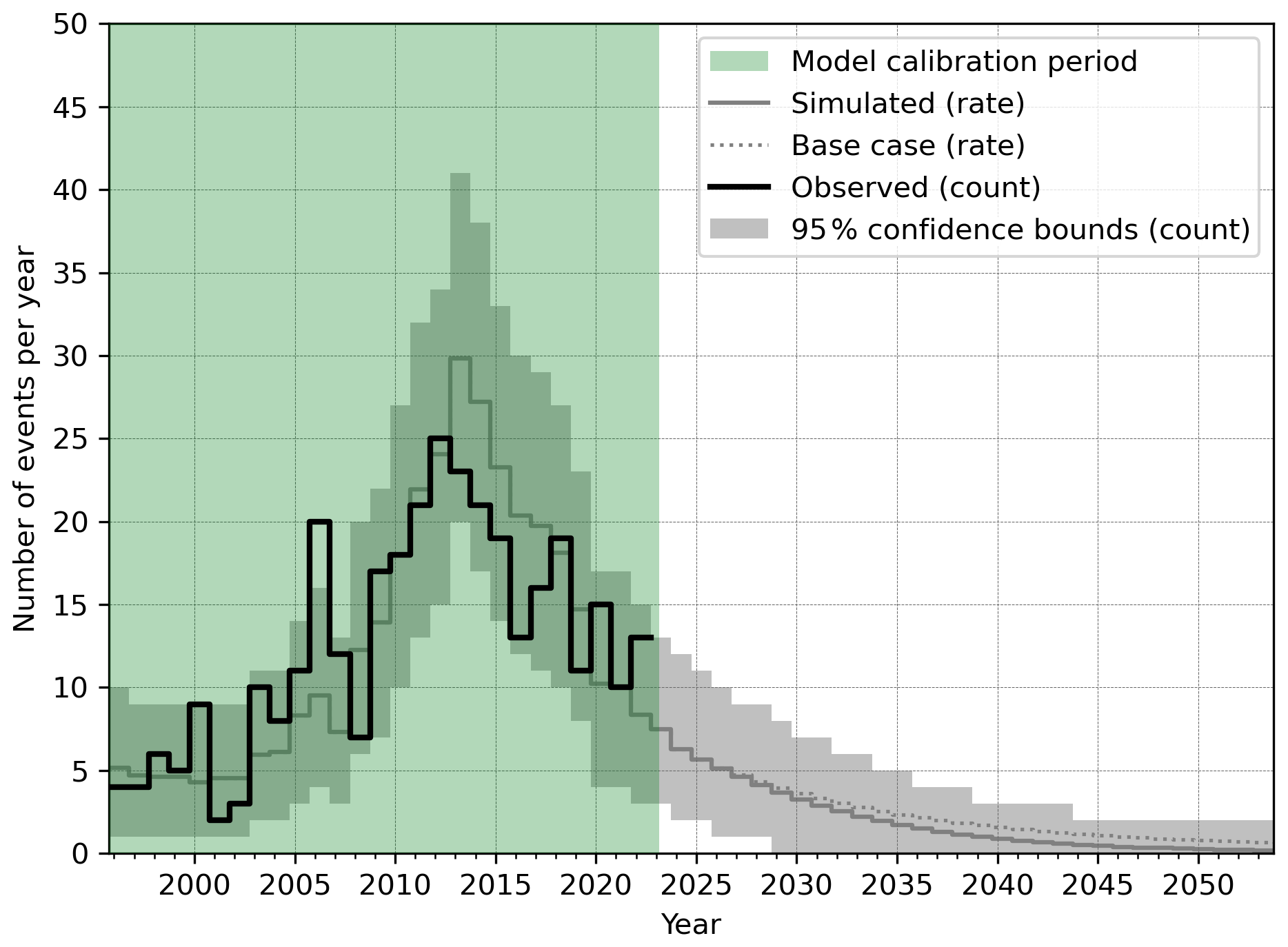
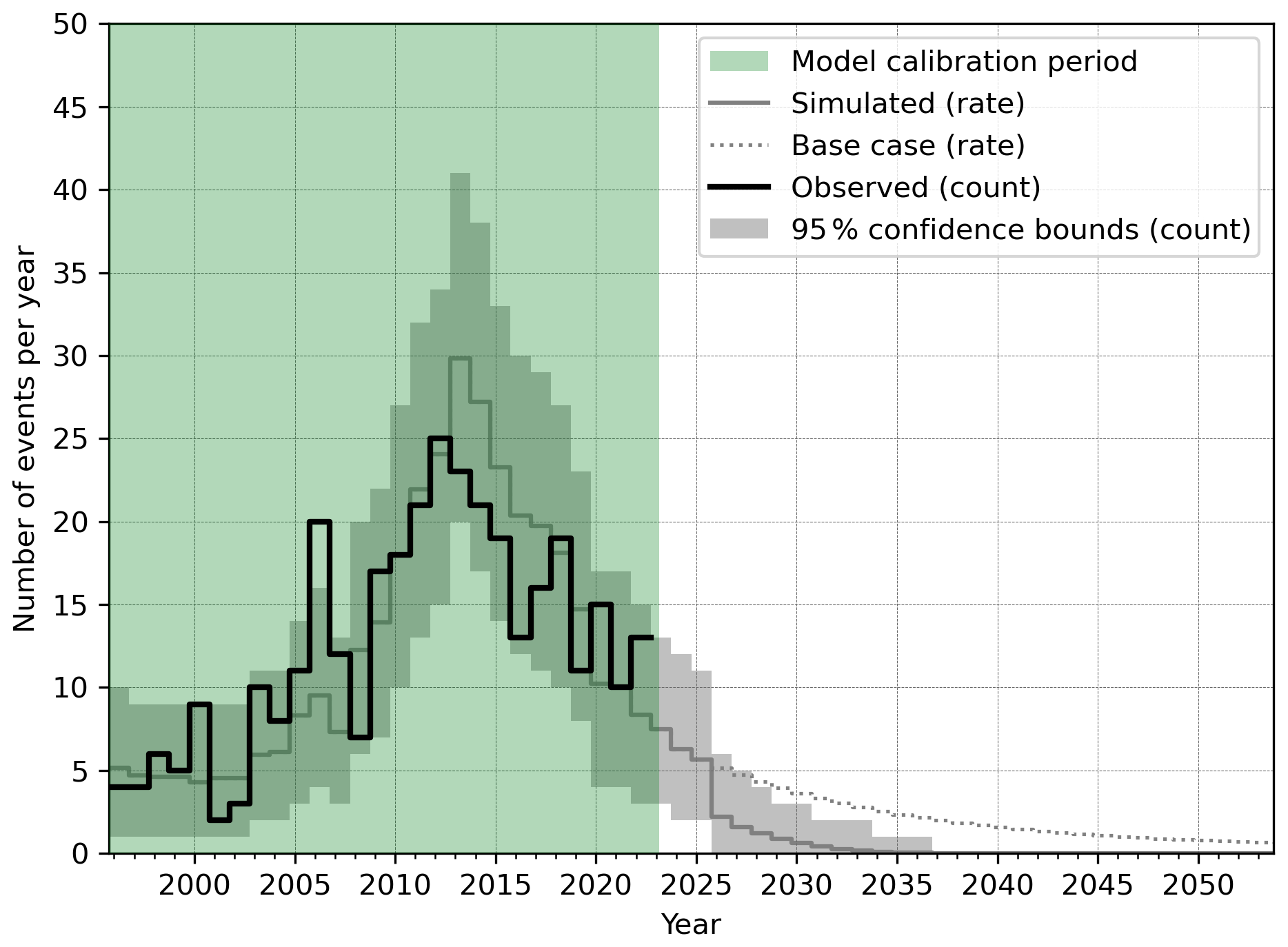
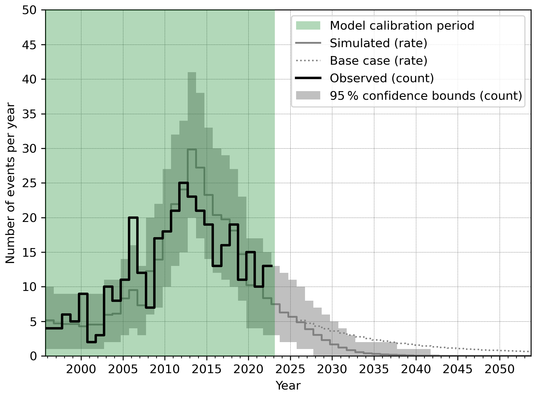
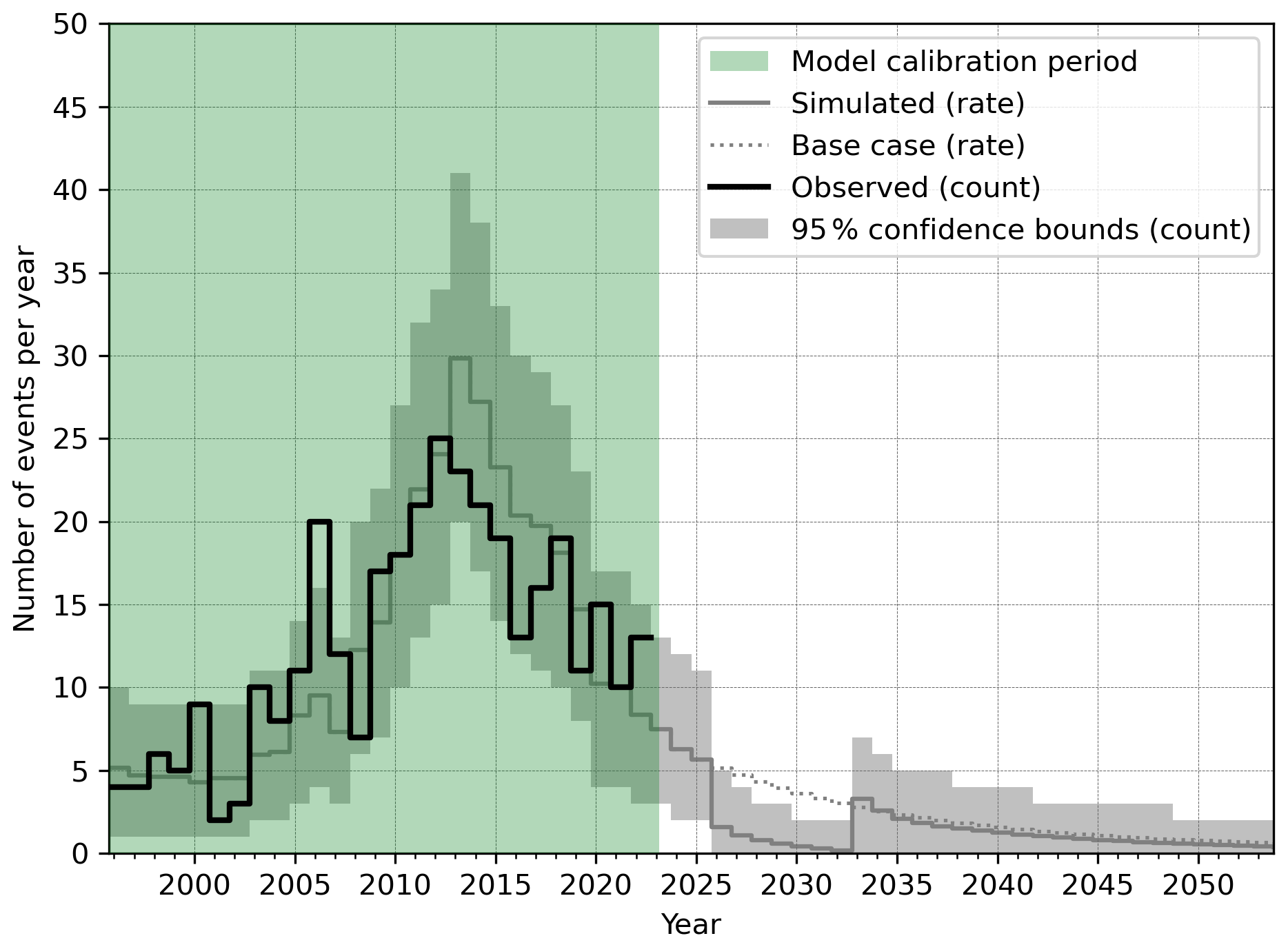
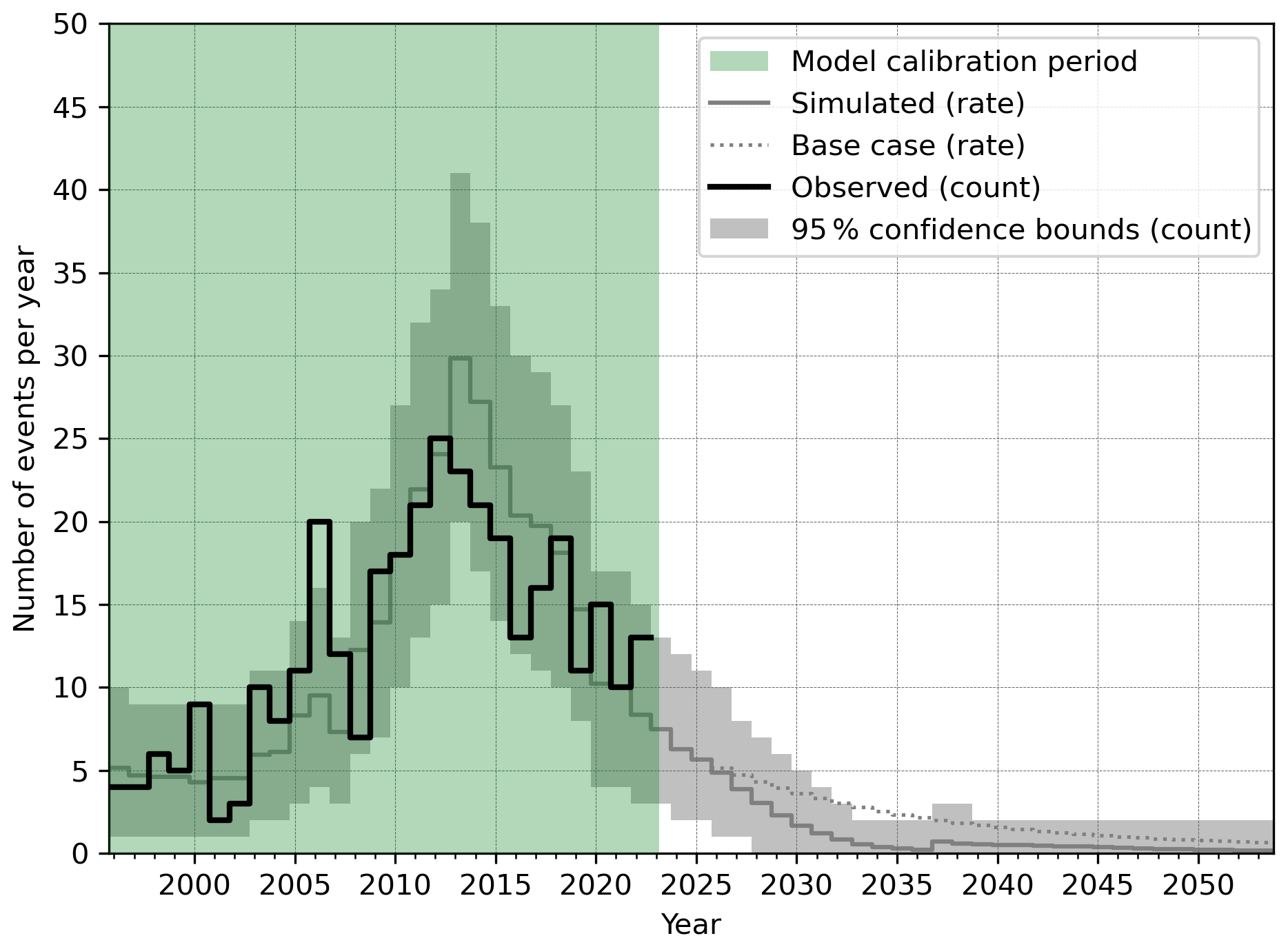
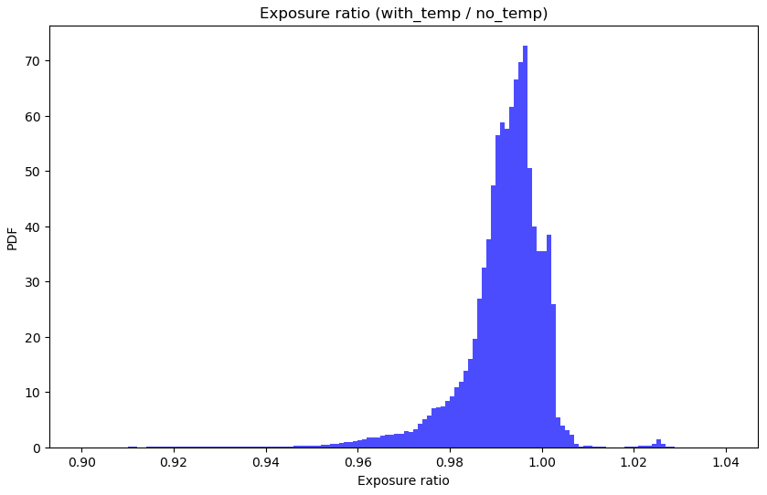
Figure A10 Ratio between risk level (Local Personal Risk) computed with temperature effects and without temperature effects. For each building, for each year in the forecast, and for each scenario we obtain a ratio. We show this as a single histogram, combining all the annual data of all scenarios in a single plot. In general, the risk level computed per building with temperature effects is a few percent lower than without temperature effects due to the slightly lower levels of seismicity. However, for some select buildings the ratio is slightly above unity. The main take-away is that the effect of accounting for temperature effects is very minor.