Benefits of the simplified MEV for analyzing hourly precipitation extremes in a changing climate

Predicting the likelihood of extreme hourly rainfall events is crucial in mitigating risks associated with flash floods and related hazards. Previous research shows that, for limited sample sizes, the simplified Metastatistical Extreme Value (sMEV) distribution can significantly reduce the associated uncertainty in rainfall return levels compared to the more commonly used General Extreme Value (GEV) distribution. Recent research also highlights the possibility to analyze the effects of climate change using the non-stationary versions of both distributions. Thus, we investigate the sMEV and GEV distributions for hourly precipitation obtained from a convection-permitting regional climate model. The global climate model MIROC5 is employed to drive the regional climate model COSMO over the greater Germany area for historical, near-future and far-future periods. This comparison is novel in combining a large spatial and temporal extent with a high spatial and temporal resolution. The results show that, in the current climate, the GEV method estimates on average higher return levels than the sMEV for hourly extremes. However, this difference reverses with further global warming. The results also reveal, that the sMEV outperforms the GEV in the sensitivity to small samples across almost all return periods regardless of the length of observational records. In addition, there is a north-south gradient in the return level difference, the uncertainty difference and crucially the adequacy of the sMEV left-censoring threshold. In addition, we investigate non-stationary versions of the sMEV and GEV under climate change. The chosen non-stationary sMEV shows more promise in describing the change in return levels compared to the non-stationary GEV. However, both non-stationary versions analyzed lack complexity and should be used carefully when projecting future rainfall extremes.

1 Introduction

Precipitation extremes on an hourly time scale can trigger natural hazards, such as debris flows, land slides, flash floods and urban flooding (Golz et al., 2016). Quantifying the probability of events of a certain magnitude is crucial for engineers, insurers, spatial planners and policymakers. However, such assessments are challenging due to the lack of observational data at sub-daily time scales (Valipour, 2016; Pritchard et al., 2023; Poschlod et al., 2021). Furthermore, climate change is already altering the intensity and frequency of extreme precipitation events (Zeder and Fischer, 2020; Lang and Poschlod, 2024; Haslinger et al., 2025), with further increases projected under continued warming (Prein et al., 2017; Fowler et al., 2021; Myhre et al., 2019). Thus, there is a need for robust and accurate methodologies to estimate extreme rainfall intensities and frequencies (Martel et al., 2021).

Due to the limited availability of observational records of hourly precipitation, climate models are increasingly used to enhance our understanding of local climate dynamics. In the mid-latitudes, hourly rainfall extremes are typically related to convective events (Guichard et al., 2004), and accurately representing such extremes requires the explicit simulation of deep convection (Prein et al., 2015). Additionally, climate change increases hourly precipitation extremes in these regions (Lenderink and Van Meijgaard, 2008), primarily because warmer air can hold more moisture (Clausius-Clapeyron relationship), leading to a higher frequency of large, long-living convective cells (Purr et al., 2021). Recent advances in computing power have enabled to run convection-permitting climate models over decadal to multi-decadal time periods. Thus, extreme value theory can now be applied to convection-permitting climate model simulations to assess hourly precipitation extremes in a warming climate.

Extreme value theory aims to estimate the occurrence probability of rare events. There are two main approaches to achieve this goal. The first is the asymptotic approach, in which, under certain assumptions, a subset of precipitation events converges towards a specific probability density function as the sample size increases. A well-known example is the block-maxima method (Gumbel, 1958), which typically uses years as blocks and assumes that the annual precipitation maxima asymptotically follow the Generalized Extreme Value (GEV) distribution (Jenkinson, 1955). A major limitation is that the block-maxima sampling discards much of the available data that could augment the analysis - particularly when only a few years of data are available.

The alternative approach assumes that some of the precipitation values directly follow a certain probability distribution regardless of the number of observations. This differs to the more common asymptotic approach, which states that rainfall values asymptotically converge to a probability distribution over time. One such alternative method is the Metastatistical Extreme Value (MEV) approach, introduced by Marani and Ignaccolo (2015). The MEV approach sorts all precipitation data into distinct events, separated by a dry period. For each event, the maximum hourly rainfall is identified applying a moving window over the event duration. The MEV method then assumes that, within a given year, the maximum hourly precipitation values from individual rain events follow a parent distribution, where the Weibull distribution is commonly used (Marani and Ignaccolo, 2015). Building on the MEV approach, Marra et al. (2019) introduced the simplified MEV (sMEV) approach, which groups precipitation maxima of rainfall events into different classes. Then events from each class across several years are fitted to a single 3-parameter Weibull distribution. While sMEV introduces additional uncertainty by neglecting inter-annual variability, Marra et al. (2019) and Miniussi and Marra (2021) find that classifying events based on underlying processes can reduce overall uncertainty and bias compared to the MEV and GEV approach. These advantages are especially apparent when analyzing rare, short-duration precipitation extremes when only a short observation period is available (Dallan et al., 2023).

Both the GEV and sMEV approaches can account for non-stationarity by allowing their parameters to vary with time-dependent co-variates. Several co-variates, such as time or temperature, have been used to incorporate climate change effects (Schlef et al., 2023). While non-stationary versions can improve accuracy by representing temporal changes, the additional complexity may increase the uncertainty. Recently, Vidrio-Sahagún et al. (2023) compared the non-stationary versions of sMEV (NS-sMEV) and GEV (NS-GEV) for daily rainfall observations in Mexico. Their study indicates that linear NS-sMEV distributions outperform linear NS-GEV distributions in terms of fitting efficiency, accuracy, and uncertainty. Furthermore, Marra et al. (2024) showed for a case study in Switzerland that NS-sMEV distributions with a scale parameter that exponentially depends on temperature efficiently represent observed temperature scaling rates.

Despite recent advances in the development of the sMEV and NS-sMEV approaches, several knowledge gaps remain. The performance of return level estimation is highly dependent on the spatial (Araujo et al., 2023) and temporal scale, highlighting the need for further research to understand which approach should be used when (as proposed by Vidrio-Sahagún et al., 2024). In particular, studies comparing the GEV and sMEV performance for hourly precipitation over greater regions are missing. Furthermore, there are no multi-decadal studies investigating the effect of climate change on the return level estimation and uncertainty of the sMEV.

Here, we address these gaps by analyzing hourly precipitation over a Central European domain, using high-resolution, convection-permitting simulations of the Consortium for Small-scale Modeling (COSMO; Rockel et al., 2008). The simulations cover three 30-year periods, 1971–2000, 2031–2060, and 2071–2100, under a high-emission scenario. We apply both stationary and non-stationary versions of the sMEV and GEV models to assess return levels of hourly precipitation, demonstrating for the first time their applicability based on multi-decadal, convection-permitting simulations over a greater domain.

This approach allows us to investigate differences between the GEV and sMEV for hourly return level estimates, as well as their sensitivity to small samples. The latter is particularly important when estimating magnitudes of large return periods based on short observational records. Regional patterns for return level and uncertainty differences are discussed in the context of varying climate characteristics in conjunction with a fixed left-censoring threshold of the sMEV approach. Additionally, the uncertainty differences between the GEV and sMEV are investigated under varying sample sizes. The long time series used in the analysis allows us to reveal trends in return level estimates under global warming. Finally, we evaluate the benefits and limitations of the four extreme value approaches by comparing their estimates and uncertainties.

2 Study area and data

2.1 Study area

The Central European domain is centered over Germany including parts of the neighboring countries (Fig. 1a). The study area includes the northern lowlands, low and middle mountain ranges and large parts of the Alps, covering a wide variety of orographic complexity. Approximately a third of the area is covered by the North Sea and Baltic Sea in the north.

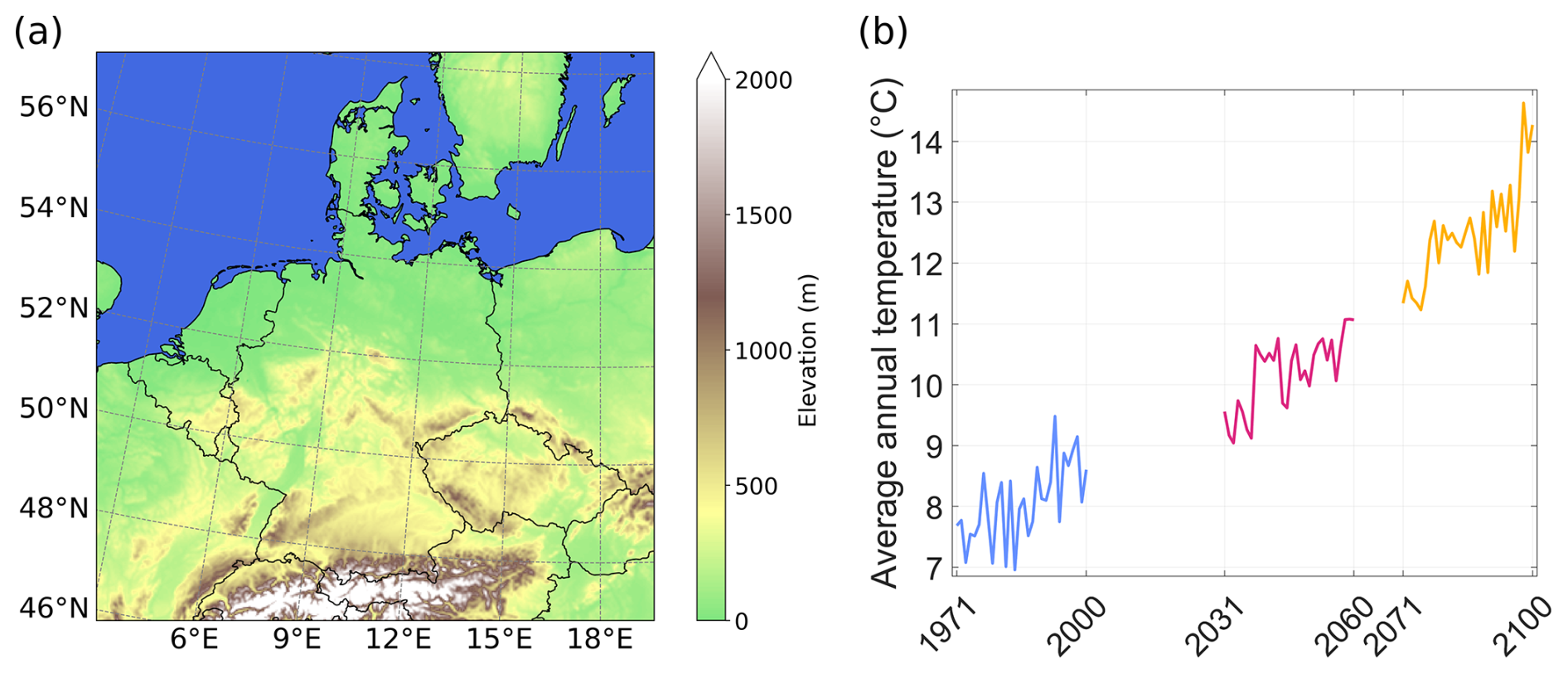
Figure 1 (a) Study area, including 425×415 grid points which are mapped using a rotated pole projection. (b) Time series of the mean annual temperature averaged over the study area considering three 30-year periods.

Using the Köppen-Geiger climate classification, the region can be divided into three distinct climate zones (Beck et al., 2018). The western and northwestern areas are characterized by a temperate climate without dry seasons and warm summers (Cfb). Most of the northeastern, eastern and southeastern areas have warm summers and no dry season, but are classified as cold climates (Dfb). The southern regions covering the Alps fall partly within the subarctic (Dfc) and polar tundra category (ET) (Fig. S8). The entire study area is regularly affected by extra-tropical cyclones and convective rain events (Ulbrich et al., 2009; Hawcroft et al., 2012; Pacey et al., 2023; Taszarek et al., 2020). Its relatively humid conditions (Zomer et al., 2022) lead to a large number of rainfall events. The number and relative intensity of these events are of particular importance in the sMEV method (Marra et al., 2018).

2.2 Data

We use convection-permitting simulations of the regional climate model COSMO (Rockel et al., 2008). The boundary conditions stem from the Model for Interdisciplinary Research on Climate (MIROC5) under the high-emission scenario RCP8.5 (Riahi et al., 2011). This scenario spans a wide range of regional warming levels, allowing analysis beyond weak warming conditions. It leads to a drastic temperature increase over the domain (Fig. 1b). However, recent literature suggests that future warming levels will likely stay below this scenario (Hausfather and Peters, 2020).

MIROC5 resolves the atmosphere horizontally for the entire globe at a scale of ∼1.4° (Watanabe et al., 2010) and has been found to represent the Central European climate well (McSweeney et al., 2015). The downscaling is carried out for three time periods, 1971–2000, 2031–2060, and 2071–2100, using a two-step nesting strategy with an intermediate nest of ∼12.5 km and the final resolution of 0.0275° (∼3 km) for our study area (Rybka et al., 2023). This scale allows to resolve deep convection explicitly while shallow convection is still parameterized (Purr et al., 2019). Here, deep convection refers to storms which extend throughout the whole troposphere and are characterized by strong upward winds. Shallow convection refers to convective processes in which clouds extend only up to around one kilometer in elevation (Arya, 2001).

Driven by boundary conditions of the ERA5 reanalysis, Rybka et al. (2023) find good agreement between hourly return levels derived from COSMO, radar measurements and rain gauge data over Germany. However, the COSMO model has a slight tendency to overestimate hourly extremes. This overestimation is particularly pronounced at higher elevations (Dallan et al., 2023), obscuring the reverse orographic effect. This effect refers to the observed decrease in annual maxima of hourly precipitation in highly elevated areas with complex terrain, such as the Alps (Allamano et al., 2009; Avanzi et al., 2015).

3 Methods

The analysis is performed using both stationary and non-stationary versions of the sMEV and GEV distributions. The software for the statistical analysis, written in Matlab R2023b, is based on previous work by Marra (2020) and Marra and Peleg (2023). Certain smaller functions, like inversion or optimization routines, are used with minor modification. However, the greater framework of the analysis is entirely rewritten. For more information see the “Code availability” section.

All parameters are estimated using the method of L-moments, which allows for a more robust parameter estimation compared to the maximum likelihood estimation. In comparison, the L-moment method has reduced sensitivity to outliers (Poschlod, 2021) and places a greater emphasis on the tail of the distribution (Hosking, 1990). The distributions are fitted to hourly precipitation separately at individual grid cells of the COSMO simulation, amounting to a total of 175 545 fits across the study area. Note that other parameter estimation methods include regional information in local estimations. This information expansion serves to spatially smooth parameter estimates and, as a result, return level estimates as well (Hosking and Wallis, 1997; Blanchet and Lehning, 2010; Schellander et al., 2019). In turn, results are spatially less noisy and potentially more robust. However, these methods have the potential of hiding local extreme value characteristics. Additionally, for real world application such regional data may not always be available.

After estimating the parameters, we calculate return levels for return periods between 5 and 200 years. In addition, we compare the sensitivity to small samples of the GEV and sMEV distributions using the relative root-mean-square error (RRMSE) for different sample lengths and return periods. For each sample length smaller than 90 years, we generate artificial datasets by repeatedly bootstrapping the available years similar to Zorzetto et al. (2016). The entire 90-year time series (1971–2000; 2031–2060; 2071–2100) defines the benchmark return levels RL_true(RP), by which the RRMSE is measured. Note that the estimated return levels are not compared to a ground-truth which is based on real-world observation, but instead to return levels estimated using a longer climate model time series. For a sample length “SL” and a return period “RP”, the estimated return level ${\mathrm{RL}}_{\mathrm{estim}}^i(\mathrm{SL},\mathrm{RP})$ is calculated n=100 times with $i\in \mathit{\{}\mathrm{1},\mathrm{\dots },n\mathit{\}}$. For a specific “SL” and “RP”, the RRMSE is defined by:

$$\begin{array}{}\text{(1)}& \begin{array}{rl}\mathrm{RRMSE}& (\mathrm{SL},\mathrm{RL})\\ & =\sqrt{{\displaystyle \frac{\mathrm{1}}{\sqrt{n}}}\sum _{i=\mathrm{1}}^n{\left({\displaystyle \frac{{\mathrm{RL}}_{\mathrm{estim}}^i(\mathrm{SL},\mathrm{RP})-{\mathrm{RL}}_{\mathrm{true}}\left(\mathrm{RP}\right)}{{\mathrm{RL}}_{\mathrm{true}}\left(\mathrm{RP}\right)}}\right)}^{\mathrm{2}}}.\end{array}\end{array}$$

Note that bootstrapping years from all time periods destroys their serial correlation and neglects non-stationary due to climate change. However, the purpose in calculating the RRMSE is to assess the variations in uncertainties across different distributions, spatial domain, sample lengths, and return periods. Compared to these variations, effects introduced by climate change are relatively small, with relatively small variation in the RRMSE under global warming (see Figs. S12, S13 and S14). Thus, we choose to ignore the temporal trends to focus on other types of variability.

3.1 GEV

The stationary GEV is widely used in rainfall extreme value statistics (Martins and Stedinger, 2000; Villarini and Smith, 2010; Cheng et al., 2014; De Paola et al., 2018; Merz et al., 2022; Gentilucci et al., 2023). It is based on the block maxima sampling approach, whereby the maximum value within a specified time block – typically one year – is selected for analysis. Specifically, we assume that inter-annual hourly rainfall maxima are independent and identically distributed. According to the Fisher–Tippett–Gnedenko theorem (Fisher and Tippett, 1928; Gumbel, 1954), the distribution of annual maximum hourly rainfall (RX1h) converges to the GEV distribution for a sufficiently large number of years. For the GEV distribution, any return period (RP) has the associated return level (RL) of

$$\begin{array}{}\text{(2)}& {\mathrm{RL}}_{\mathrm{RP}}=\mathit{\mu }-{\displaystyle \frac{\mathit{\sigma }}{\mathit{\zeta }}}\left(\mathrm{1}-{\left(-\log \left(\mathrm{1}-{\displaystyle \frac{\mathrm{1}}{\mathrm{RP}}}\right)\right)}^{-\mathit{\zeta }}\right),\forall \mathit{\zeta }\ne \mathrm{0}.\end{array}$$

Here, the location parameter μ∈ℝ determines the center of the distribution, the scale parameter $\mathrm{0}<\mathit{\sigma }\in \mathbb{R}$ controls the spread, and the shape parameter $\mathit{\zeta },\in \mathbb{R}$ governs the tail of the distribution, respectively. This method has the advantage that for intra-annual precipitation events no underlying probability function has to be assumed.

In a warming climate, the assumption that annual maxima arise from identical distributions is no longer valid. To account for this non-stationarity, the parameters of the GEV can be modeled as function of a co-variate. Here, we use the mean annual near-surface temperature averaged over the study area (Fig. 1b) as co-variate. The choice of the spatial domain is motivated by Keune and Miralles (2019), who found that most moisture supplying precipitation over Central Europe originates from local sources. Since we are interested in the long-term effect of global warming on precipitation, the mean annual temperature is an adequate representation of climate change.

Following Vidrio-Sahagún et al. (2023) and Agilan and Umamahesh (2017), we introduce non-stationarity by modeling the location parameter as a linear function of temperature $\mathit{\mu }\left(t\right)={\mathit{\mu }}_{\mathrm{0}}+{\mathit{\mu }}_{\mathrm{trend}}\cdot \stackrel{\mathrm{̃}}{T}$. This parsimonious version avoids the sensitivity associated with making the scale and shape parameters temperature-dependent (Cheng et al., 2014). Furthermore, the inclusion of only one additional parameter increases the computing load only slightly. While simplified, it provides a reasonable estimate of how extreme hourly precipitation is affected by temperature changes (De Paola et al., 2018).

3.2 sMEV

The block maxima approach using annual values requires a relatively large sample size to mathematically justify the use of the GEV distribution, which can lead to large estimation uncertainties for short records (Veneziano et al., 2009). To address this limitation, the sMEV approach was developed by Marra et al. (2020), based on previous work by Marani and Ignaccolo (2015) and Marra et al. (2019). This approach can also be interpreted as a block maxima method; however, here the blocks correspond to independent rainfall periods separated by dry intervals. The maximum hourly rainfall for each rainfall period is called an ordinary event (Fig. 2b). The method further assumes that all ordinary events across several years can be separated into groups. Each group follows a certain probability distribution reflecting the underlying physical processes.

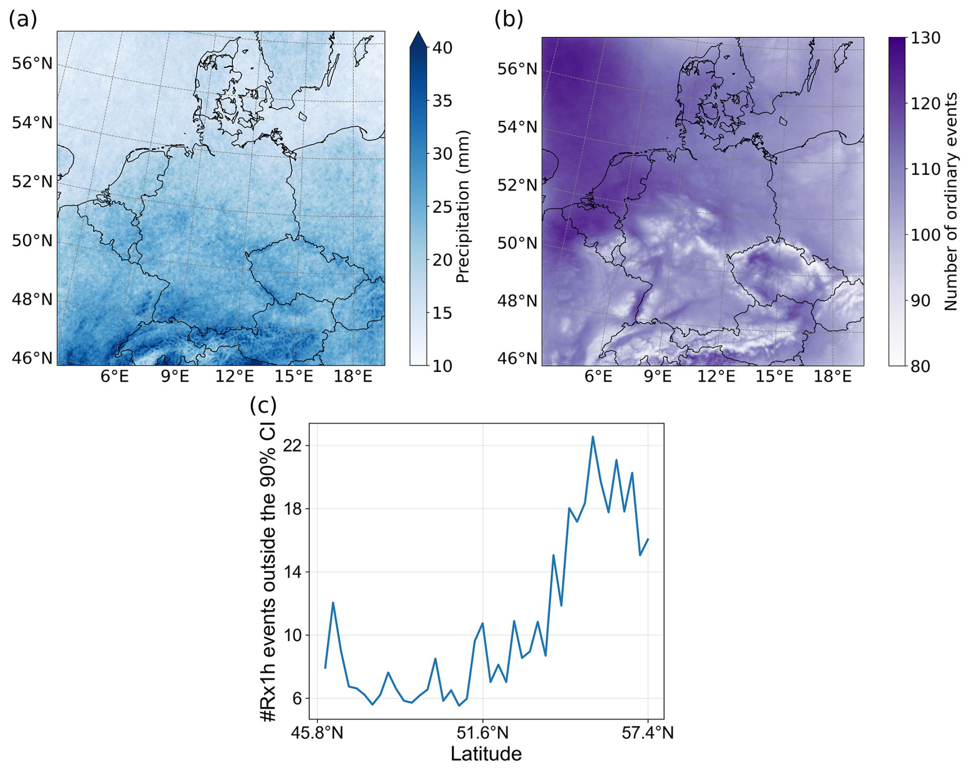
Figure 2 Average RX1h magnitude (a) and average annual number of ordinary events (b) over the study area. Number of RX1h events in the dataset, averaged over the latitudes, that fall outside the 90 % interval of the sMEV using the 95th percentile as threshold for ordinary events (c). All sub-plots refer to the full 90-year time series.

For the event separation, we choose 12 h as the minimum dry period between events, which is a slightly more conservative choice compared to Marra et al. (2020). Additionally, we focus on the upper quantile of ordinary hourly rainfall events within each year. Thereby, we assume that all events in this fixed upper quantile are governed by the same physical processes. This is a reasonable assumption for a sufficiently large threshold, since Barbero et al. (2019) showed that in the mid-latitudes, annual maxima of hourly rainfall precipitation are primarily a result of short convective storms.

The Weibull distribution is a good choice when modeling heavy-tailed sub-daily rainfall extremes, as it is heavy tailed if the inverse shape parameter $\mathrm{0}<\mathit{\omega }<\mathrm{1}$ (Marra et al., 2018). The return level (RL) for any return period (RP) can be expressed as

$$\begin{array}{}\text{(3)}& {\mathrm{RL}}_{\mathrm{RP}}=C{\left(-\log \left(\mathrm{1}-{\left(\mathrm{1}-{\displaystyle \frac{\mathrm{1}}{\mathrm{RP}}}\right)}^{\frac{\mathrm{1}}{\overline{n}}}\right)\right)}^{\frac{\mathrm{1}}{\mathit{\omega }}}\end{array}$$

Here, $\mathrm{0}<C,\mathit{\omega }\in \mathbb{R}$ are the scale and the inverse shape parameter, respectively, and $\mathrm{0}<\overline{n}\in \mathbb{R}$ is the average number of ordinary events per year.

The upper quantile must be determined carefully, as including low-intensity events may not be representative of hourly precipitation extremes, whereas including too few events leads to large uncertainties (Wang et al., 2020). To determine an appropriate left-censoring threshold for the ordinary events, we use a test proposed by Marra et al. (2020). This test iteratively evaluates the likelihood that the observed RX1h values arise from a specific left-censored sMEV distribution. Starting with a very low left-censoring threshold $p\in [\mathrm{0},\mathrm{1})$, the sMEV is fitted to all ordinary event greater than the p-quantile. Based on this sMEV distribution, $\overline{n}\times N$ events are randomly sampled, with the maxima across $\overline{n}$ yielding N RX1h events. Repeating this random sampling many times yields the 90 % confidence intervals of the nth largest RX1h values $\forall n\in \mathit{\{}\mathrm{1},\mathrm{\dots },N\mathit{\}}$. Next, the proportion of actual RX1h values falling within this confidence interval is assessed. If the number of events outside the confidence interval is larger than 10 %, the loop is repeated with an incrementally larger left-censoring threshold. Otherwise, this left-censoring threshold is chosen as the ideal value and the loop ends. In our case, this corresponds to the 95 % percentile. For consistency, we choose the 95th percentile as the left-censoring threshold for the whole study area, as a constant threshold makes it easier to compare and interpret the uncertainty of the sMEV approach across the spatial domain.

Applying this test with the 95 % threshold reveals a pronounced north-south gradient. In the central and southern parts of the study region, less than 10 % of the RX1h values fall outside the 90 % confidence interval, whereas this proportion can exceed 20 % in regions north of 53° N (Fig. 2c). This pattern indicates that a greater number of events could be considered in the south while still satisfying the test criteria, whereas higher thresholds would be required in the north (see also Fig. S3). Thus, our choice of threshold limits the number of grid points which fail the test, while at the same time maximizes the number of available data points.

The optimal threshold is expected to vary across climatic regions, and different studies have adopted different values accordingly. For example, Marra et al. (2019) use the 75th percentile for Israel, while Miniussi and Marra (2021) choose the 90th percentile for daily precipitation in Germany. Similarly, Wang et al. (2020) select the 90th percentile for hourly precipitation of five rain gauges in western Germany, and Dallan et al. (2023) and Marra et al. (2024) apply the 90th percentile for hourly and sub-hourly precipitation in northern Italy and Switzerland, respectively. Our chosen threshold is higher than those in comparable studies, likely reflecting the moist climatic conditions of our study area which is characterized by many low-intensity rainfall events. However, it may also reflect methodological differences, such as our use of simulation data for grid cells of approximately 9 km² rather than station data.

Marra et al. (2019) introduced a variation of the sMEV distribution to account for non-stationarity in the underlying data. Following Vidrio-Sahagún et al. (2023), we investigate the NS-sMEV formulation in which the scale parameter C and the number of ordinary events n depend on the spatially averaged annual temperature $\stackrel{\mathrm{̃}}{T}$. However, instead of a linear relationship we adopt the approach of Marra et al. (2024) and model the scale parameter as an exponential function of temperature, such that $C=C_{\mathrm{0}}{e}^{C_{\mathrm{1}}\cdot \stackrel{\mathrm{̃}}{T}}$, while the number of events depends linearly on temperature, i.e. $\overline{n}=n_{\mathrm{0}}+n_{\mathrm{1}}\cdot \stackrel{\mathrm{̃}}{T}$ with $C_{\mathrm{0}},C_{\mathrm{1}},n_{\mathrm{0}},n_{\mathrm{1}}\in \mathbb{R}$. Marra et al. (2024) showed that the exponentially temperature-dependent scale parameter effectively reproduces the observed Clausius-Clapeyron relationship.

Introducing non-stationarity into probability distributions can substantially increase the computing power required for parameter estimation. Moreover, adding variables raises the risk of overfitting. For both the NS-GEV and NS-sMEV, we therefore adopt simple non-stationary formulations, while choosing the relationships most likely to capture the change in return levels with increasing temperatures. Based on Vidrio-Sahagún et al. (2023) and Marra et al. (2024), this is a linear dependence of the GEV location parameter, while other parameters are kept constant. For the sMEV distribution the shape parameter is kept constant, while the scale parameter is exponentially dependent on temperature. Calculating the number of ordinary events is computationally inexpensive; hence, we also allow this parameter to vary with temperature without significantly increasing the computational burden. We have confirmed the added value of these non-stationary distributions applied to the whole dataset by calculating the corrected Akaike’s information criterion, similar to Kim et al. (2017) (Fig. S15). Compared to stationary distributions the non-stationary distributions have a smaller value for the corrected Akaike’s information criterion and thus add value when applied to this dataset.

4 Results

4.1 Comparison of stationary GEV and sMEV

Across the study area, the GEV location and scale parameters generally increase with time, indicating an increase of extreme precipitation in a warmer climate (Fig. 3a). Relative to the historical period, the spatially averaged location parameter increases by 10 % and 28 % in the near and far future, while the mean scale parameter increases by 17 % and 29 %, respectively. In contrast, the shape parameter shows a slight decrease due to climate change, with the spatial mean around 0.15. It also exhibits high spatial variability, with an inter-quartile range between 0 and 0.3 for all three periods. The largest contribution to the increase in return levels comes from the increasing scale parameter, which directly amplifies extreme precipitation magnitudes (Fig. S1 in the Supplement).

For the sMEV distribution, the mean inverse shape parameter decreases from 0.52 in the historical period to 0.49 in the far future (Fig. 3b). The scale parameter slightly decreases from 0.7 (1971–2000) to 0.67 (2031–2060) before increasing to 0.73 in the far future. The average annual number of ordinary events decreases only slightly over time, from around 110 in the past period to around 108 in both future periods. The main driver of temporal changes in sMEV-based return levels is the decrease of the inverse shape parameter, as lower values translate into higher extremes (Fig. S1).

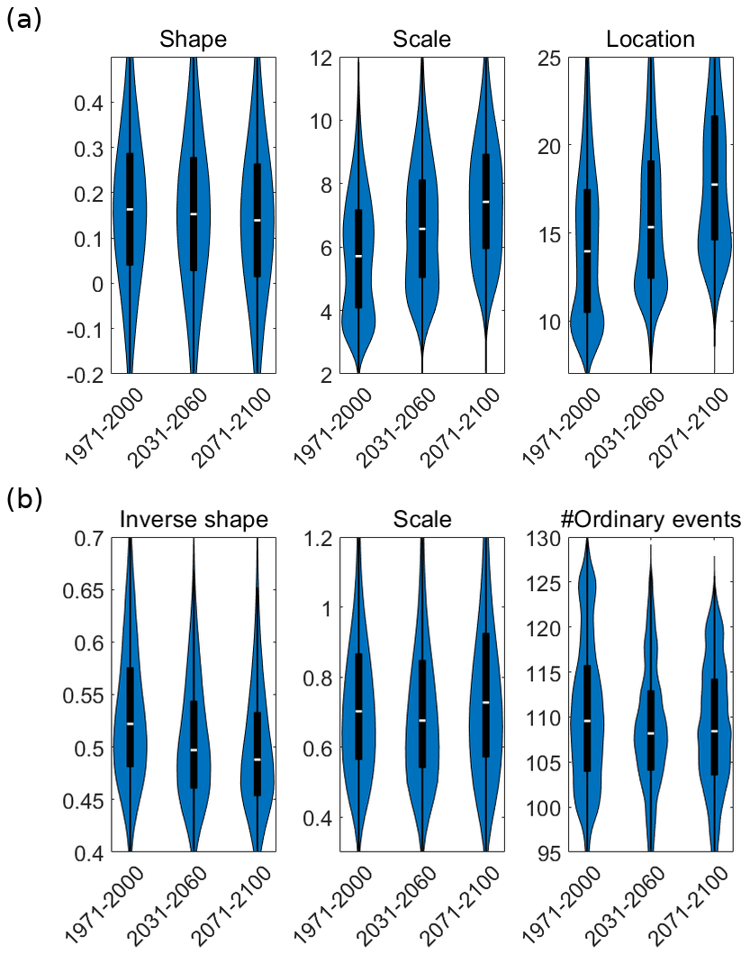
Figure 3 GEV parameters (a) and sMEV parameters (b) for different time periods. The violin plots show the shape, scale, and location parameters of the GEV and the inverse shape, scale, and number of ordinary events of the sMEV across the study area. The blue area is defined by a kernel density distribution with the black bar marking the 25th and 75th quantiles, while the white marker indicates the mean values.

These parameter changes result in increasing return levels when spatially averaged over the study domain (Fig. 4a and b). The GEV and sMEV agree for moderate return periods of 10 years or less, but begin to diverge at higher return periods (Fig. 4c). Specifically, the sMEV tends to estimate lower return levels in the past, but higher return levels in the far future compared to the GEV. However, the median difference between the two approaches remains below 10 %.

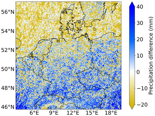
We find a distinct spatial pattern in the return level difference between sMEV and GEV (Fig. 4d). For the 100-year return level and the past period, the return level difference shows a clear north-south gradient: GEV estimates are higher in the north, while sMEV return levels are higher in the south. This pattern becomes even more pronounced in the future time periods (Fig. S2). Although this spatial pattern holds for all return periods (see Figs. S9 and S10), it is less distinct for lower return periods.

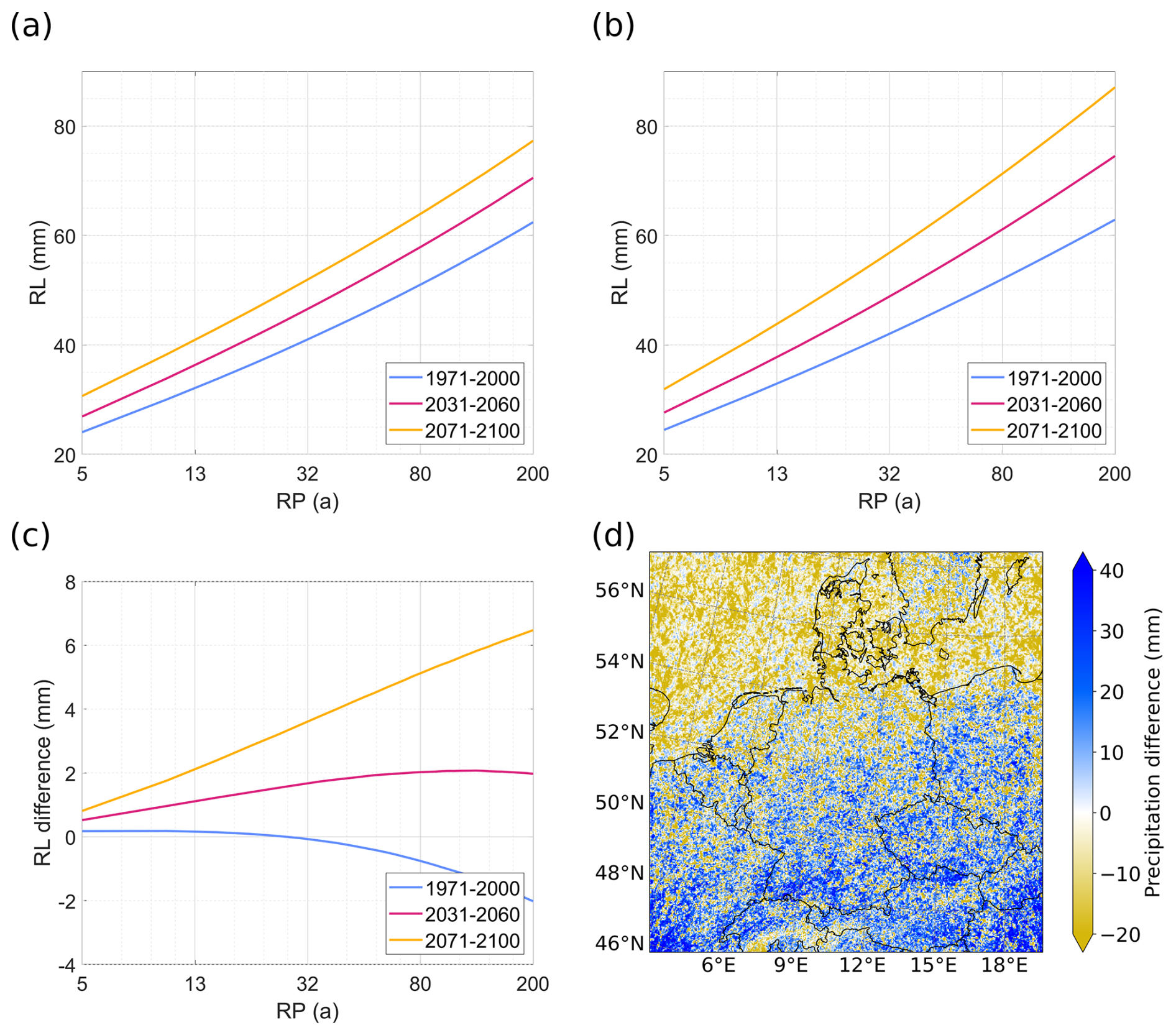
Figure 4 Spatially averaged return levels (RL) of the GEV (a) and sMEV (b) for different return periods and time periods. Difference in the spatial median return level of sMEV and GEV (c). Difference in the 100-year return level of sMEV and GEV for the period 1971–2000 (d).

Next, we calculate the temperature scaling of the return levels for each grid point, using the historical period as the baseline. Scaling is expressed per degree of warming for the 10-year and 100-year return periods, with temperature defined as the average value over the whole domain for each time period. For both return periods, the GEV approach yields a mean temperature scaling of around 6 % (Fig. 5a). The sMEV approach yields higher average scaling: around 8 % for the 10-year and around 10 % for the 100-year return period (Fig. 5b). For both approaches and both return periods, the spatial variability decreases when considering the difference in the first and third time period compared to the first and second. For the 10-year return period, both approaches yield similar spatial variability. For the 100-year return period, the sMEV approach has a significantly lower spread of scaling parameters.

The spatial distribution of the temperature scaling rate is shown using the 10-year return level as an example. Both the GEV (Fig. 5c) and sMEV (Fig. 5d) exhibit a similar north-south gradient with higher scaling rates in the north of the study region and smaller values towards the south. An exception is the Alps region, which shows higher scaling rates compared to other locations at similar latitudes. Compared to the sMEV, the GEV exhibits slightly higher scaling rates in the northern sea regions and slightly lower values in the center of the study domain, as well as smaller values around the Alps region (Fig. S11).

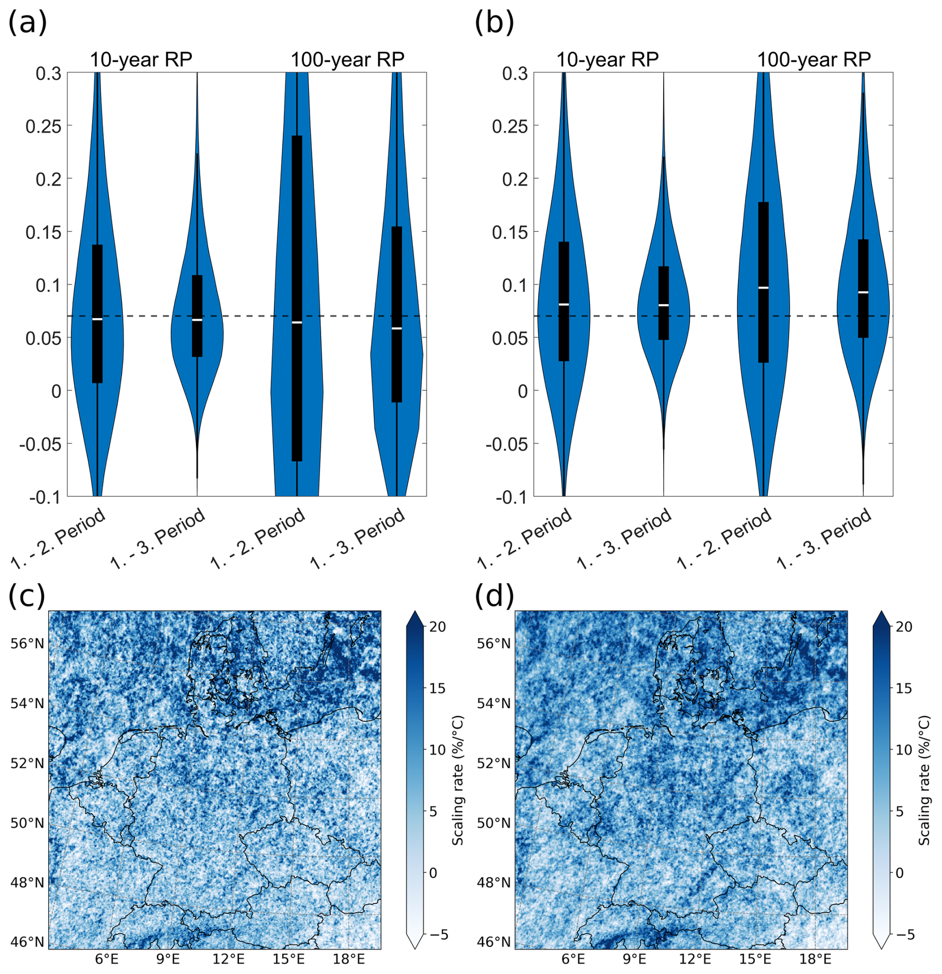
Figure 5 Temperature scaling for the 10-year and 100-year return levels for the GEV (a) and sMEV (b) approach across the study area. For Fig. (a) and (b) the y-axis shows the relative change of the return level per degree of warming, based on the 30-year average temperature of each period. The temperature scaling is shown for the difference between the first and second period as well as the first and third period. Black bars mark the 25th and 75th quantiles with the white marker showing the mean. The dashed line indicates the Clausius-Clapeyron scaling of 7 % °C⁻¹. Panels (c) and (d) display the 10-year return level change per degree of warming for the GEV (c) and sMEV (d) approach. The rate of change is calculated based on the return levels of the periods 2071–2100 and 1971–2001.

The sensitivity to small samples for varying return level estimates is quantified by the relative root-mean-square error (RRMSE). Here, the return levels derived by considering the whole 90-year time series serve as ground-truth. Both GEV and sMEV generally have a relative error below 10 % when the sample size exceeds the return period for which the return levels are estimated (Fig. 6a and b). The GEV shows a slight increase in relative error with larger return periods, whereas the sMEV is less sensitive to the return period, except for very short return periods. Furthermore, the GEV performs poorly when the sample length is smaller than 25 years, with relative errors far exceeding 100 %. The ratio of the sMEV and GEV RRMSEs (Fig. 6c) highlights that the two methods yield similar errors only for very small return periods and relatively large sample sizes. For return periods larger than 25 years and sample sizes greater than 30 years, the GEV has approximately double the relative error. For small sample sizes, the sMEV strongly outperforms the GEV, often by several orders of magnitude. The spatial pattern of the RRMSE ratio is similar to the difference in return levels. For the case of the 100-year return period and 30-year sample size, which is representative for most combinations, sMEV yields a relative error that is ∼3 times smaller in the north and ∼2 times smaller in the south compared to the GEV (Fig. S4).

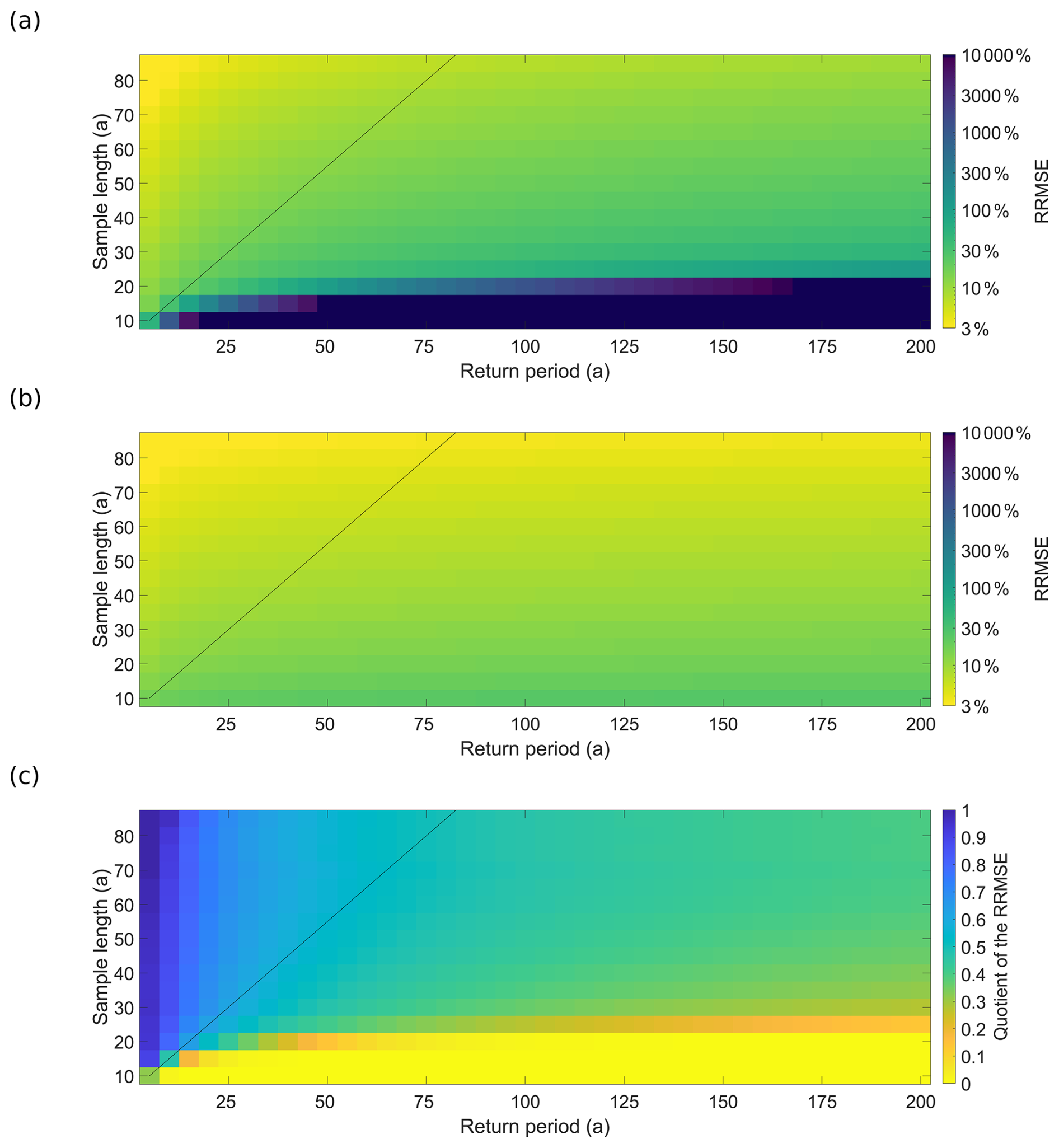
Figure 6 Relative root-mean-square error (RRMSE) as function of sample size and return period for the GEV (a) and sMEV (b). Ratio of the RRMSE values of sMEV and GEV (c). A ratio around 1 (dark blue) indicates that the GEV and sMEV have similar RRMSE values. Values around 0.1 (yellow) indicate that sMEV performs around ten times better. The calculation is based on bootstrapping the respective sample length 100 times from all available years.

4.2 Comparison of non-stationary GEV and sMEV

Both non-stationary approaches were fitted to the individual time periods as well as the entire 90-year time period (Fig. S5). The spatial mean 100-year return level is used to visualize the difference for the NS-GEV (Fig. 7a, solid lines) and NS-SMEV (Fig. 7b) solid lines). When fitted to 30-year time periods the 100-year spatial mean return levels of the NS-GEV are consistently higher than for the stationary GEV (Fig. 7a, dashed lines). Meanwhile, the NS-SMEV shows more agreement in spatial mean 100-year return levels compared to the stationary SMEV (Fig. 7b, dashed lines).

Furthermore, when the non-stationary distributions are fitted to the entire available time series (combining 1971–2000, 2031–2060, and 2071–2100) the predicted 100-year return levels differ to the distribution fitted to individual time periods within their respective temperature range. Both distributions predict higher average return levels for lower temperatures and lower average return levels for higher temperatures. This low sensitivity to temperature is more visible for the NS-GEV compared to the NS-SMEV. While the 100-year return level was used as an example, the previous statement applies on average to all other return levels (Fig. S6). Moreover, Fig. 7c shows that in absolute terms the return level difference between the NS-GEV and NS-SMEV are on average larger for greater return periods.

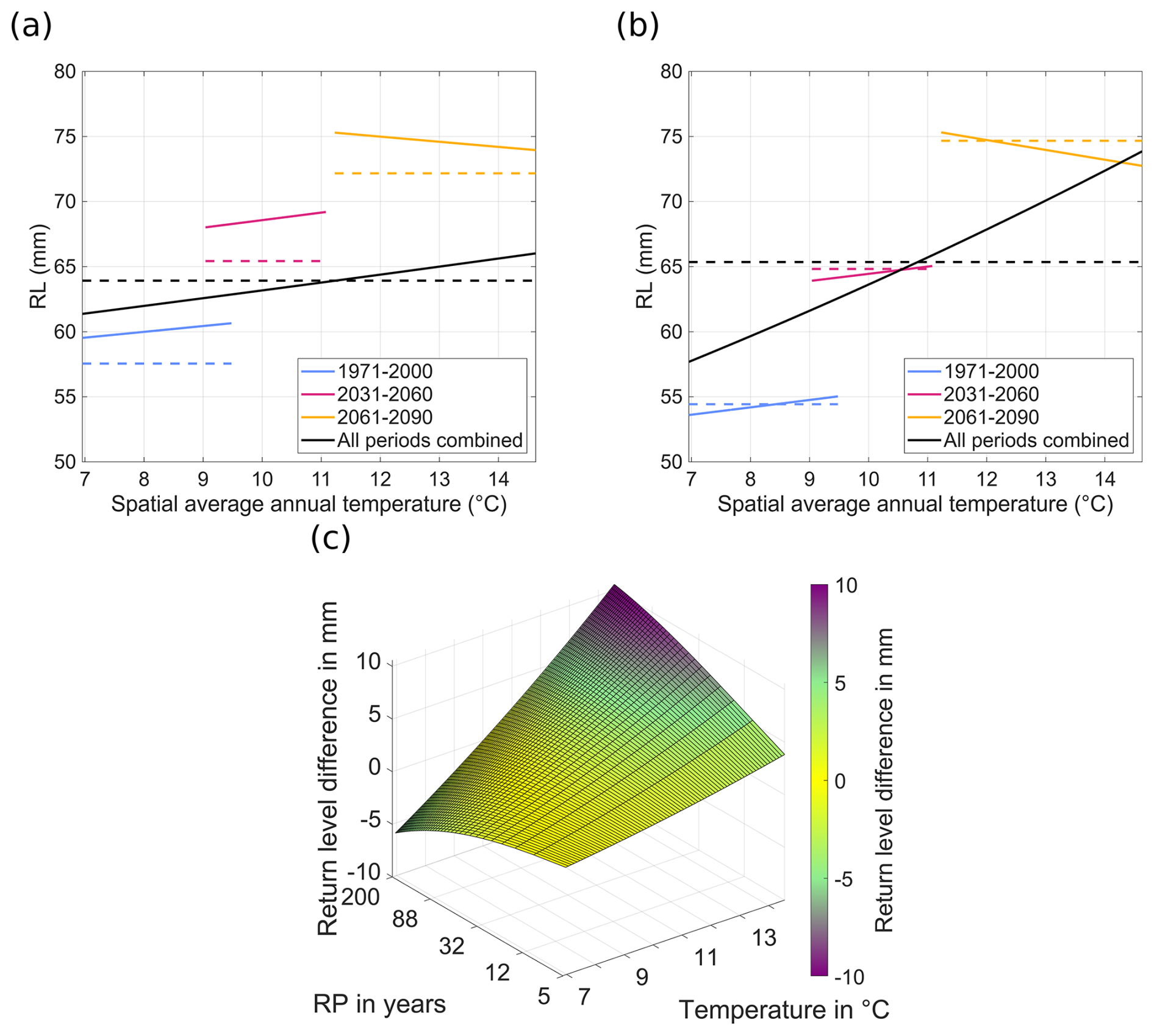
Figure 7 The 100-year return levels, averaged over the study area, of the NS-GEV (a) and NS-sMEV (b). Solid lines denote the 100-year return levels of four non-stationary distributions fitted to each respective time period and to the combined time period. Dashed lines are the respective return levels of the stationary distributions. Each plot is constraint to the annual spatial average temperatures values present in the respective time period. Average return level difference of the NS-sMEV and NS-GEV when both are fitted to the entire time series (c).

5 Discussion

5.1 Stationary distributions

First, it is important to characterize the alterations of distribution parameters under climate change. For lower return periods the scale and location parameter of the GEV are both causing an increase of similar magnitude, while the change in the shape parameter can be neglected (Fig. S1). For higher return periods the location and shape parameter cause an opposite effect of similar magnitude, while the scale parameter causes a significantly larger increase. It is a noteworthy result that the median shape parameter of the GEV is decreasing, making the distribution less heavy-tailed (Fig. 3a). This is in stark contrast to the sMEV approach. Here the median distribution gets more heavy-tailed causing a significant increase in the return levels, particularly for high return periods. The change in the scale parameter is comparably small, while the change in the number of ordinary events can be neglected entirely. The difference between both approaches indicate that the relationship between annual maxima changes in a fundamentally different way to the relationship of the largest 5 % of ordinary events throughout the time periods.

Comparing the return levels derived by the stationary models, we observe that for the past period the GEV generally provides higher return levels than the sMEV. However, in a warming climate, this pattern seems to reverse, with the sMEV predicting relatively higher return levels. This behavior is governed by a temperature scaling of the GEV which is slightly below the Clausius-Clapeyron-scaling of 7 % °C⁻¹, with the sMEV being slightly above it (Fig. 5). This combines with the spatial north-south gradient in differences between the sMEV and GEV (Fig. 4d). Our results show a similar pattern to Rybka et al. (2023) which analyzed scaling rates of the 10-year return level for 3-hourly rainfall extremes. Their results are derived using the peak-over-threshold method and are constraint over Germany (Fig. 8 in Rybka et al., 2023). Similar to our results they find higher scaling rates in the north of Germany, however our results show higher scaling rates on average, which is in part due to our study domain being larger.

The spatial patterns shown in Figs. 4d and 5c and d rare closely linked to the climatological characteristics of the study domain. The northern regions generally have lower elevations (Fig. 1a), have more ordinary events and smaller hourly rainfall extremes (Fig. 2), governed by an oceanic climate. In the south, the annual rainfall is significantly higher, enhanced locally by orographic lifting while governed by a continental climate. These southern regions also experience higher temperatures during the extended summer season, when convective events mostly occur.

In order to understand what role these climatic factors might play, we emphasize that the sMEV considers more than just the largest annual rainfall value. This is done under the assumption that all ordinary events stem from the same physical processes. Figure 2c shows the test which evaluates the adequacy of the 95 % left-censoring threshold. It reveals that in the northern latitudes, the largest annual hourly precipitation value deviates more often from the assumed distribution. The change in the curve along the latitude is quite abrupt and matches with the spatial pattern of the differences in return level and uncertainty. The likely cause of this geographical variability is that the number of ordinary events considered by the sMEV is higher in the northern regions. In turn, the events that are considered are less likely to be a result of deep convection as the process causing the most extreme precipitation in Central Europe (Arakawa, 2004). As a result, the sMEV estimates lower return levels for large return periods in the northern regions (Fig. 4d). Due to the more intense RX1h events in the South, there is a southwards increase in return level differences. Additionally, climate change affects the moist northern region of the study domain differently to the relatively dryer south. Accordingly, both the GEV and sMEV approach estimates that higher temperature scaling rates in the north of the study domain. However, the GEV estimates higher scaling rates in the maritime north, while the sMEV estimates higher scaling rates in the continental center of the domain.

While our analysis highlights the spatial and climate change-related discrepancies between sMEV and GEV and discusses possible reasons, the exact cause remains unclear. We emphasize that there is a high sensitivity to the climatic conditions (spatially and under climate change) when comparing the sMEV to the GEV. More research and more applications of the sMEV to different climates are needed to fully understand what drives this shift. We also recommend further research on the choice of the sMEV left-censoring threshold for a more robust application on regional to continental scales.

Further applications of sMEV are beneficial, as the sMEV is able to estimate accurately return levels of small probabilities based on small samples (Fig. 4). This is in line with the results for daily precipitation over Austria from Schellander et al. (2019). However, unlike Schellander et al. (2019), in our study, the estimation skill of the sMEV does not deteriorate with larger return periods. Furthermore, in opposition to Schellander et al. (2019), the GEV is outperformed even if the sample size is greater than the return period to be predicted. The spatial distribution of the RRMSE contributes to explaining these differences. Generally, the GEV shows higher uncertainties in the north compared to the sMEV, whereas the lowest uncertainties are diagnosed over Austria. In turn, the spatial distribution of the RRMSE of the sMEV is homogeneous (Fig. S4). Hence, within our study area, the GEV shows its best performance over Austria compared to the sMEV. Still, our findings indicate that the sMEV may be even more beneficial for hourly extremes than for daily extremes when rare return levels are needed. For moderate extremes up to 10-year events, the GEV performs just as well as the sMEV (Fig. 4). Based on these findings, the variability of the RRMSE differences between the GEV and sMEV is mainly driven by the variability of the GEV.

5.2 Non-stationary distributions

For the NS-GEV, the spatial average return level is higher compared to the stationary GEV when only 30 years are used to fit the distribution (Fig. 7a). This is likely driven by the relatively high RRMSE of the GEV (Fig. 6c) coupled with the additional uncertainty that is introduced by adding another parameter in the NS-GEV. This increased uncertainty makes large outlier values more likely, causing the upward shift in average return levels. This increasing trend is much less prevalent when the spatial median return levels are considered (Fig. S7). In contrast, the average and median return levels of the NS-sMEV are much more similar (Figs. 7b and S7).

The different sensitivities to increasing temperature in Fig. 7 are mainly driven by the varying design of the NS-GEV and NS-sMEV (also see Fig. S6). The NS-GEV depends linearly on temperature, while the NS-sMEV is affected both linearly and exponentially. Moreover, for the NS-GEV, a linearly dependent location parameter does not represent the change in return levels well (Fig. S6). In fact, the scale parameter should also be non-stationary when trying to capture the effects of climate change, because the scale parameter has a greater effect on the tail of the distribution (Fig. S1). However, as noted earlier, this might amplify the comparatively large RRMSE of the GEV.

For the NS-sMEV the change in the number of ordinary events has little impact on the change in return levels (Fig. S1). Thus the change in return levels is mainly driven by the exponentially dependent scale parameter. The changing scale parameter is somewhat able to capture some of the increase in return levels with warmer temperatures (Fig. 7b), despite the inverse shape parameter initially impacting the return levels the most. Yet, we still have a significantly lower sensitivity when the the distribution is fitted to all time period instead of the individual ones.

In general, the accuracy of the NS-sMEV and NS-GEV in capturing climate change related changes in extreme precipitation are closely related to accurately capturing the temperature scaling rate shown in Fig. 5. Studies from Berg et al. (2019), Poschlod and Ludwig (2021) and Lenderink et al. (2021) indicate complex and non-linear behavior of temperate scaling rates for very strong climate change scenarios. In particular, Lenderink et al. (2021) indicate that over central Europe the average temperature scaling rate of the 99th percentile of hourly precipitation is slightly larger than 10 %. Thus, comparing scaling rates of the GEV and sMEV for our simulation, the sMEV is more aligned to other results. In combination with the more complex design of the NS-sMEV makes it likely that the NS-sMEV does a better job capturing changes in extreme precipitation caused by a strong global warming. However, for weaker warming trends more simple or linear non-stationary distributions may be adequate.

This case study is motivated in part by Vidrio-Sahagún and He (2022) and Marra et al. (2024) which highlight the potential for applying non-stationary sMEV distributions under climate change. Vidrio-Sahagún et al. (2023) is one of few studies comparing the NS-sMEV to the NS-GEV. This study applies the most promising and simple non-stationary versions of the GEV and sMEV to investigate behavior under climate change. While the NS-sMEV does show promising results, neither non-stationary version captures the increase in return levels well. Thus, they are not suited for estimating long term changes in return level. More research is needed for more complex non-stationary versions to better account for the changes of extreme precipitation in a warmer climate. As fitting uncertainty increases with increasing complexity, the robust sMEV framework offers a suitable base for further investigation.

5.3 Limitations

We identify four key sources of uncertainty that govern the findings of our study and any projections of extreme precipitation. These are the internal climate variability, the model uncertainty, the scenario uncertainty (Wu et al., 2022) and the statistical assumptions inherent in the extreme value distributions.

We do not have a quantification of the internal climate variability since we use a single COSMO run (Kay et al., 2015). Poschlod and Ludwig (2021) find that the temperature scaling of 10-year return levels varies between 4 % °C⁻¹ and 15 % °C⁻¹ over Central Europe. Given that their findings are based on a 50-member single model initial-condition large ensemble of a regional climate model parameterizing deep convection, the uncertainty range is higher for convection-permitting simulations (Chen et al., 2021) and rarer return periods. Many modes of climate variability influence extreme rainfall that are not well sampled with such short time periods. For example, the north Atlantic oscillation exhibits significant cycles with 34 years in length Seip et al. (2019). Furthermore, our data record includes temporal gaps, which may lead to incomplete coverage when analyzing the time periods that are available. An ensemble of model runs with slightly different initial conditions could mitigate this uncertainty (Kendon et al., 2020).

Moreover, the COSMO model does not simulate real-world climate conditions perfectly. For instance, Haller et al. (2021) have shown that the COSMO model slightly overestimates hourly precipitation extremes compared to KOSTRA estimates. The KOSTRA approach estimates rainfall return levels based on historic rain gauge data (see Malitz and Ertel, 2015; Junghänel et al., 2017; Shehu et al., 2023). Also different climate models show deviations in the projection of future rainfall extremes in a warmer climate (Berg et al., 2019). This uncertainty could be mitigated by performing a similar study with a multi-model ensemble (Fosser et al., 2024).

Furthermore, we are only considering the high-emission RCP8.5 climate scenario. This is the most extreme future scenario used by the IPCC (Pachauri et al., 2015). We cover regional warming levels of up to 7 °C for the average annual temperature (Fig. 1b), which might be considered as unrealistically strong warming. However, the strong warming poses the greatest challenge for the non-stationary distributions.

Finally, we must recognize the statistical assumptions made when developing the statistical distributions. We have already pointed out some of the assumptions made when applying the GEV and sMEV in Sect. 3. For the sMEV, we assume that all ordinary events stem from the same physical processes. Thereby, the choice of the left-censoring threshold induces uncertainty. Focusing on the MEV approach Serinaldi et al. (2025) show how assuming an explicit parent distribution for a subset of all events can be error prone. The authors also show, how neglecting inter-annual variability is especially problematic when few observational years are available, which puts the relative advantages of the sMEV approach into perspective. For the GEV, we assume that all hourly annual maxima are “extreme”, which might be not the case in every year. Implicitly, we apply the Fisher-Gnedenko-theorem on small sample sizes even though it only holds for sufficiently large samples.

In general, estimating large return levels from few observational years is highly uncertain regardless of the extreme value method used. In reality, great care should be taken when estimating large return levels in such a way. The sensitivity to small samples may seem relativity small in case of the sMEV. However, the true range of uncertainty may be far greater, if the previously mentioned assumptions are not met. Thus, especially the results based on a 30-year sample size should be viewed with this limitation is mind (for instance Figs. 4 and 5). Moreover, small sample uncertainty and method uncertainty may have varying importance depending on the location and return level. For instance, when estimating a 100-year return level with 30 years of observations, the spatial average RRMSE of the GEV and sMEV is 34.6 % and 12.5 %, respectively, while the return level differences tend to be lower in the center of the study domain and regularly exceed 40 % towards the extreme north or south (see Fig. 4d).

As mentioned, the application of non-stationary extreme value distributions are potentially subject to large uncertainties. By applying the NS-GEV to discharge data, Serinaldi and Kilsby (2015) highlighted the dangers of erroneously assuming non-stationarity. More generally, the authors provide an in depth discussion on the pitfalls of applying non-stationary extreme value distributions in practice. Furthermore, we assume that regional near-surface temperature is a suitable co-variate to describe the change in return levels due to climate change, which is motivated by other studies but not following our physical understanding. Ultimately, despite some assumptions being hurt, the applied extreme value distributions are a useful tool to assess occurrence probabilities of hourly extreme precipitation. Still, they always remain a simplifying description of reality.

6 Conclusions

This study presents a comprehensive analysis of extreme hourly precipitation under future climate change conditions using convection-permitting climate model simulations. Both stationary and non-stationary versions of the GEV and sMEV are assessed in terms of their accuracy and robustness in estimating hourly rainfall return levels. Our findings highlight several key differences between the GEV and sMEV distributions, notably their deviating sensitivity to spatial variability and climate change. While we can confirm the robustness of the sMEV framework on small sample sizes, we further find higher accuracy for hourly precipitation extremes compared to the GEV. However, we identify limitations of the approach demanding further research. A careful selection of the left-censoring threshold and its sensitivity to different climatic conditions might require spatially varying threshold choices. This would induce additional complexity, uncertainty, and limited comparability across the study domain, but could improve the performance of the sMEV.

Our results show that the simple non-stationary implementation of the NS-GEV fails to capture the strong changes in extreme precipitation under the high-emission scenario, whereas the NS-sMEV better accounts for these dynamics. However, neither of the chosen non-stationary distributions are able to fully capture the effect of climate change on extreme precipitation. It is likely that more degrees of freedom in the non-stationary parameters of the distributions are necessary to improve the ability of capturing the effect of climate change. Such extensions will inevitably cause a super-linear increase in the computing power necessary to fit the parameters. Moreover, the uncertainty is expected to increase alongside the number of parameters. A decision framework, such as that proposed byVidrio-Sahagún et al. (2024), can guide the selection of statistical approaches based on user-specific circumstances.

We suggest that future research on the choice of the left-censoring threshold and on refining non-stationary statistical models cover various regions and data sources to address open questions in the sMEV framework. Priorities include: (a) conducting regional to continental studies to assess the challenges and benefits of a spatially varying left-censoring threshold, (b) applying the sMEV on single model initial-condition regional climate model ensembles to explore the sensitivity to internal climate variability, (c) applying the sMEV on multi-model climate model ensembles to examine the sensitivity to model uncertainty, and (d) refining non-stationary sMEV versions based on convection-permitting climate model ensembles to overcome the limitations of small sample sizes.