the Creative Commons Attribution 4.0 License.
the Creative Commons Attribution 4.0 License.
 | 10 Mar 2023
Human influence on growing-period frosts like in early April 2021 in central France
Robert Vautard
Geert Jan van Oldenborgh
Rémy Bonnet
Yoann Robin
Sarah Kew
Sjoukje Philip
Jean-Michel Soubeyroux
Brigitte Dubuisson
Nicolas Viovy
Markus Reichstein
Friederike Otto
Iñaki Garcia de Cortazar-Atauri
In early April 2021 several days of harsh frost affected central Europe. This led to very severe damage in grapevine and fruit trees in France, in regions where young leaves had already unfolded due to unusually warm temperatures in the preceding month (March 2021). We analysed with observations and 172 climate model simulations how human-induced climate change affected this event over central France, where many vineyards are located. We found that, without human-caused climate change, such temperatures in April or later in spring would have been even lower by 1.2 ∘C (0.75 to 1.7 ∘C). However, climate change also caused an earlier occurrence of bud burst that we characterized in this study by a growing degree day index value. This shift leaves young leaves exposed to more winter-like conditions with lower minimum temperatures and longer nights, an effect that overcompensates the warming effect. Extreme cold temperatures occurring after the start of the growing season such as those of April 2021 are now 2 ∘C colder (0.5 to 3.3 ∘C) than in preindustrial conditions, according to observations. This observed intensification of growing-period frosts is attributable, at least in part, to human-caused climate change with each of the five climate model ensembles used here simulating a cooling of growing-period annual temperature minima of 0.41 ∘C (0.22 to 0.60 ∘C) since preindustrial conditions. The 2021 growing-period frost event has become 50 % more likely (10 %–110 %). Models accurately simulate the observed warming in extreme lowest spring temperatures but underestimate the observed trends in growing-period frost intensities, a fact that yet remains to be explained. Model ensembles all simulate a further intensification of yearly minimum temperatures occurring in the growing period for future decades and a significant probability increase for such events of about 30 % (20 %–40 %) in a climate with global warming of 2 ∘C.
- Article
(3538 KB) - Full-text XML
-
Supplement
(707 KB) - BibTeX
- EndNote


Frost days and cold spells are decreasing in frequency and intensity worldwide (IPCC, 2021; Van Oldenborgh et al., 2019). Yet, severe cold spells continue to pound many mid-latitude areas, due to the occasional invasion of polar air being transported well into lower latitudes as a consequence of the chaotic motion of Rossby waves. When occurring in spring, such cold events can create a range of impacts on agriculture such as in April 2021, when young leaves and flowers had started to develop into fruit trees or grapevines. The frost event which took place from 6 to 8 April 2021 was exceptional, with daily minimum temperatures below −5 ∘C recorded in several places. In several places, such low temperatures left no chance to save grapevines and fruit trees with frost management strategies (e.g. local heating from braseros or spreading water to keep frost moderate at the surface of plants). The cold temperatures led to broken records at many weather stations (see Fig. 1b). Unfortunately, this cold event happened a week after an episode of record-breaking high March temperatures in many places in France and also in western Europe (Fig. 1a). This sequence caused the growing season to start early, with bud burst occurring in March and the new leaves and flowers left exposed to the deep frost episode that followed.
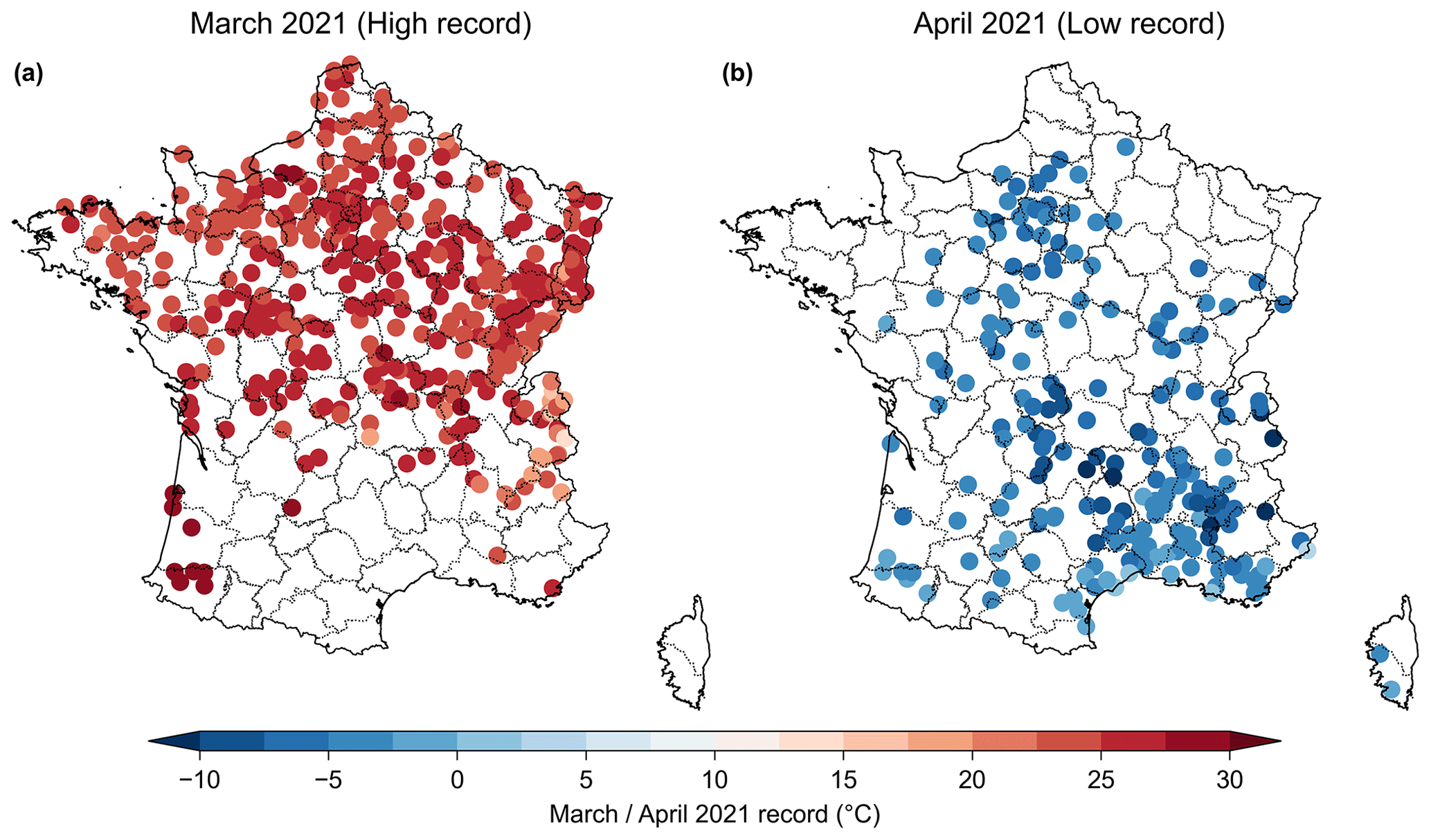
Figure 1Stations with March (a) high records broken (pink thermometer) and April (b) low records broken (since at least 20 years) (blue thermometers) in 2021 in France. Symbols are superimposed with the record value of the temperature.
In 2021, wine production had been historically low, with 33 billion hectolitres produced, a level that is 25 % below the average production of the previous 5 years and that is lower than the 2017 production, which was also hit by a late frost (AGRESTE, 2021). Beyond the frost and its consequences, the losses were amplified by a relatively cool and wet summer season allowing for mildew and Botrytis development. In general early varieties in vineyards were affected by frost (for example sauvignon in Bordeaux). The losses were widespread, but the frost hit the vineyard differently. In the hardest hit places such as Burgundy or Jura, about two-thirds of the production was destroyed. In other places such as the Beaujolais, later-developing species made the losses less severe. In the Champagne vineyards, and in many places across France, the losses ranged from 30 % to 50 % (AGRESTE, 2021).
Fruit production was also severely hit for some fruits. Estimates of production losses are of about 50 % for pears and cherries, ∼25 % for peaches, and ∼20 % for apples (with large departures from averages depending on the region). Some other productions were also impacted (such as sugar beet emergence), but final yields were not finally affected because of favourable production conditions (AGRESTE, 2021).
The occurrence of such an event called for investigating the role of climate change. From a weather point of view, the event is rather classical for cold outbreaks, when air masses of polar origin invade western Europe. The large-scale flow pattern was characterized by a strong high-latitude anticyclone extending from Greenland to the northwestern European coasts, which was found among the four most recurrent or stationary North Atlantic flows (the “Greenland blocking” pattern of Michelangeli et al., 1995, and Vautard, 1990), inducing a negative value of the North Atlantic Oscillation (NAO) index. The combination of polar air advection, cloud-free sky and still long nights led to hours of intense frost. Such dynamical events are not observed to have become more frequent (Screen and Simmonds, 2013; Blackport and Screen, 2020) despite the ongoing debate on the role of narrower sea ice extent favouring the occurrence of blocking anticyclones (Barnes and Screen, 2015). However, human-induced changes in dynamical conditions, especially leading to cold outbreaks, remain largely uncertain and can be viewed from various indices (Shepherd, 2014), and their understanding would require an in-depth, dedicated analysis.
Here we perform a statistical attribution analysis of the 2021 late frosts to climate change from an impact perspective. The effects of climate change on late frosts and their consequences are complex, because several processes are in competition, in particular the earlier start of the growing season and the general regression of cold extremes and frost days (IPCC, 2021). The advance at the start of the growing season has increased the number of frost days occurring after the start of the growing season in several places worldwide, including in Europe (Liu et al., 2018). Using several indices for grapevine exposure, it has been found that the date of the last frost day has not regressed as fast as the date of the growing season start (Sgubin et al., 2018). However, so far no formal attribution study of a “growing period-frost” has been carried out to quantify the role of anthropogenic climate change in these observed trends. In order to carry out the attribution study, we use several indices and event definitions characterizing cold temperatures in the growing season and the well-established attribution methodology described in Philip et al. (2020) and Van Oldenborgh et al. (2021b).
A rapid attribution analysis was carried out in June 2021 and reported in Vautard et al. (2021, https://www.worldweatherattribution.org, last access: 15 June 2021), with several indices developed and analysed, showing that while spring frosts are generally becoming less severe and frequent, frosts occurring after the growing season start are becoming more intense due to climate change. Since then, observations were consolidated, more model data have been collected and simulation data processing were homogenized. This article reports the final results, which confirm the conclusions of the preliminary analysis.
We present several definitions of the frost event in Sect. 2 and the corresponding indices chosen. In Sect. 3, we present methods, observations and models used, and trends in observations are analysed, and in Sect. 4, results from observations and model ensembles are analysed. This is followed by a synthesis of results, a discussion and a conclusion in Sect. 5.
The cold spell of 6–8 April 2021 hit much of central and northern Europe (see Fig. 2a). However, we focus here on central/northern France in order to investigate a relatively homogeneous, mostly plain or low-elevation area (see Fig. 2b). This area (46 to 49∘ N, −1 to 5∘ E) covers most of the grapevine agriculture areas of Champagne, Loire Valley and Burgundy which were identified as specifically vulnerable regions under climate change (Sgubin et al., 2018). The area also covers regions with high crop and fruit production.
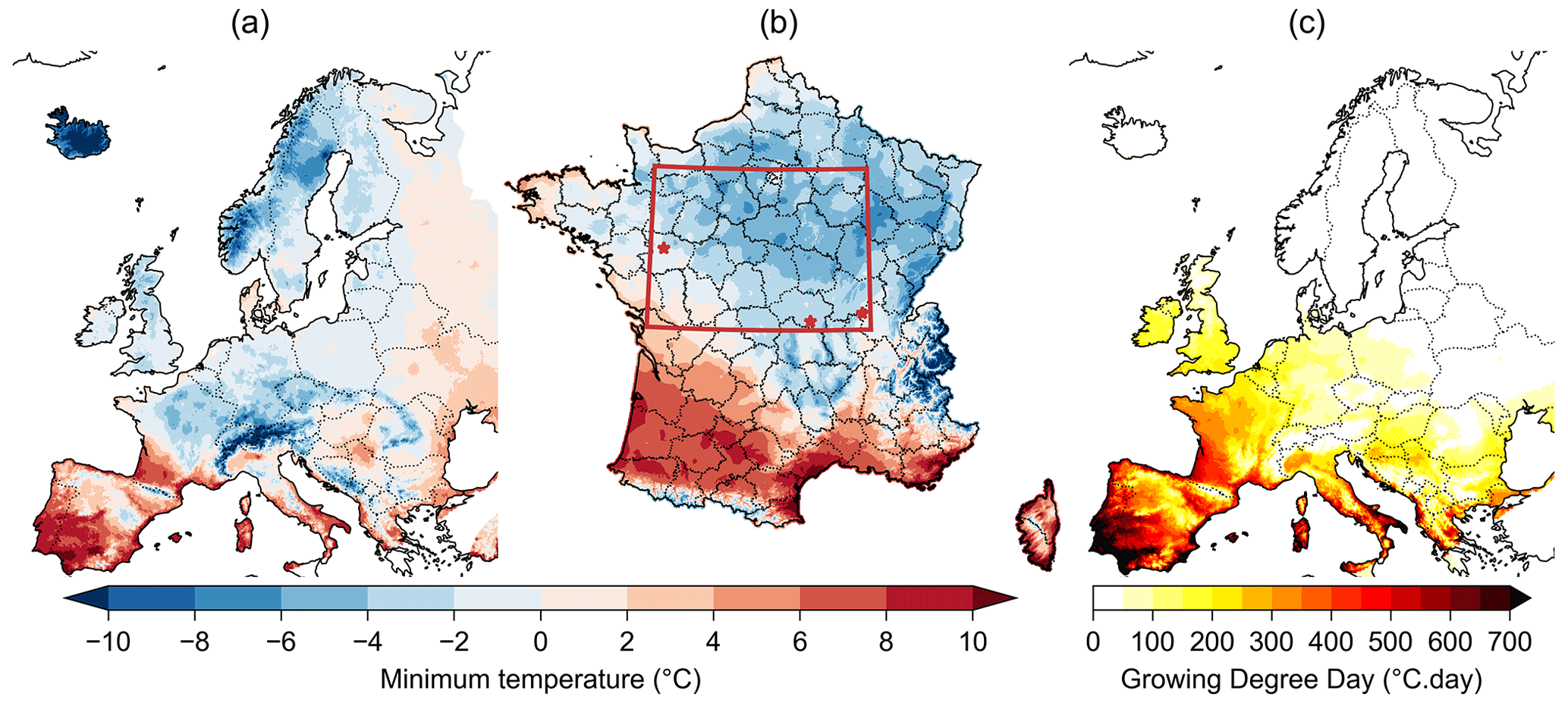
Figure 2(a) Minimum temperatures on 6 April 2021 in Europe from the E-OBS (Cornes et al., 2018) database (see Sect. 3); (b) focus on France with a higher resolution dataset, using the Anastasia data (Météo-France, Besson et al., 2019). The study area is shown in this panel by the bounded box in red; stars indicate the location of the three stations used to assess local trends; (c) spatial distribution of the growing degree day index in Europe on 5 April 2021 as calculated from E-OBS.
We use several event definitions, accounting for different phenological aspects. Differences in results for these definitions also test the robustness of the attribution. In each case, the “event” is defined as the yearly minimum temperature (TNn) obtained under specific conditions and then averaged over the area or taken at specific station locations. A basic reference conditioning is the fixed-season minimum temperature and does not consider phenology: the TNn is calculated over the April–July months (index TNnApr–Jul). The second index accounts for phenology. The TNn is calculated conditioned upon the growing degree day above 5 ∘C (hereafter denoted “GDD”) being larger than thresholds characterizing bud burst conditions, which depend on species. In this study, our aim is not to tie thresholds to specific plants' phenology but to provide a general overview for different thresholds. The GDD is calculated at each grid point with a starting date of the previous winter solstice, in a similar approach used by García de Cortázar-Atauri et al. (2009), assuming that the dormancy break period for grapes is finished in the calculation period. The formula for the GDD at day t during year y is therefore
where TM is the daily mean temperature and tstart is 21 December of the previous y year y−1 (starting time of the cumulation). In 2021, the values of the GDD obtained on the day before the frost events in the concerned area vary in the range of 150 to 350 ∘C d−1, with an average value on 5 April of 259 ∘C d−1 over the study domain. This value is high for this calendar day (rank = 14th since 1921 in the E-OBS extended dataset), but the record value was obtained in 2020, with a mean GDD of 320 ∘C d−1. Given the range of values taken in the domain, we considered 3 thresholds for GDD: 250 ∘C d−1 as a central value and 150 and 350 ∘C d−1 as sensitivity experiments. This range of values also helps to capture a range of bud burst values of grapevine cultivars as found in García de Cortázar-Atauri et al. (2009). For each GDD threshold, the yearly minimum TN values (TNn), called hereafter “TNnGDD250”, “TNnGDD150” and “TNnGDD350” for the three GDD thresholds, are calculated over subsequent days and until the end of July at each grid point and then averaged over the study area (46 to 49∘ N, −1 to 5∘ E). Despite the fact that the average characterizes the mean lowest temperature that can occur after crossing the GDD threshold, the average can mix several dates as the GDD threshold crossing, and the yearly minimum does not necessarily occur on the same date over the whole domain. In 2021, for instance, the TNnGDD250 was already reached during the 6–8 April episode for most of the area, but not in the easternmost part and in some other parts, because the GDD did not exceed 250 ∘C d−1 during the April frosts.
In order to focus on specific phenological periods when young leaves and flowers are sensitive to frost after bud burst and flowering, we also define indices over limited ranges of GDD values. The number of possibilities is large, in most cases providing qualitatively similar results. The analysis is reported here only for the range of 250–350 ∘C d−1, by using the yearly minimal temperature over this GDD range (index TNnGDD250-350). This index is again calculated at each grid point before being averaged spatially over the study region, or is taken at stations.
3.1 Methods
Event attribution methods used in this study are well documented in previous studies. The rapid attribution methodology is a classical probabilistic approach, described in Philip et al. (2020) and Van Oldenborgh et al. (2021b), and has been used in many case studies for heat waves (e.g. Kew et al., 2019; Vautard et al., 2020), extreme precipitation (e.g. Philip et al., 2018) or more complex events such as wildfire weather (Van Oldenborgh et al., 2021a). It uses a stepwise approach, analysing observations with a generalized extreme value (GEV) with a global warming index as a covariate, then it uses ensembles of models validated on the event indices and their extreme value statistics by comparison with observations, and finally it uses the GEV with the covariate fit to build a statistical model of the data under some assumptions.
In all cases (observations and models), we used data in the 1951–2021 period for the GEV fit for attribution, and for future trend estimates for a global warming of 2 ∘C, we used the period from 2000 to 2050. For observations, the covariate is the smoothed observed GISTEMP global mean surface temperature (GMST), while for models the smoothed global mean surface air temperature (GSAT) (5-year running average) is used. The only exception is the High Resolution Model Intercomparison Project (HighResMIP) SST-forced ensemble (see below), for which the observed GMST was used because of the ensemble forcing. Change statistics are calculated with respect to the year 2021 and estimated return period from observation as a reference.
3.2 Observations and model ensembles
The observations used here for the attribution are the E-OBS v23e dataset of daily minimum temperatures (Cornes et al., 2018). The above indices are calculated for each grid point, spaced every 0.25∘ in this dataset, and then averaged over the study area.
For the attribution of the frost event, we use five model ensembles. Each simulation of each ensemble was bias-adjusted using the cumulative distribution function transform (CDFt) method (Vrac et al., 2016), using the daily minimum and the daily average temperatures from E-OBS over the 1981–2020 period. Bias correction is an important step here, since GDD calculations use a threshold. This method was assessed for use in climate services in Bartók et al. (2019) and showed good performance. We used statistics of pooled ensembles, using data until 2021 for the GEV fit of the distributions. Indices are calculated exactly as for the observations: model GDD values are calculated at each grid point, using Eq. (1), and the indices are averaged over the area of study (rectangle in Fig. 2b).
The first model ensemble is the EURO-CORDEX (0.11∘ resolution, EUR-11) multi-model ensemble. It is composed of 75 combinations (as of May 2021) of global climate models (GCMs) and regional climate models (RCMs) for downscaling (see Vautard et al., 2021 and Coppola et al., 2021 for the description of the ensemble which has increased since these publications). Each simulation consists of a historical period simulation and an RCP8.5 scenario simulation with fixed aerosol concentrations. For the attribution of past evolutions historical and scenario are concatenated until 2020. Some simulations start in 1971, whereas most simulations start from 1951. Given that we need to use data from the previous year for starting GDD accumulation, all yearly indices are calculated from their second simulation year (i.e. 1972 and 1952).
The second model ensemble used to study the influence of internal variability was the IPSL-CM6A-LR model (see Boucher et al., 2020, for a description of the model and Bonnet et al., 2021, for a presentation of the ensemble). It is composed of 32 extended historical simulations, following the CMIP6 protocol (Eyring et al., 2016) over the historical period (1850–2014) and extended until 2029 using all forcings from the SSP2-4.5 scenario, with the exception of the ozone concentration which has been kept constant at its 2014 level (as it was not available at the time of performing the extensions).
The third model ensemble is a selection of the CMIP6 historical and SSP3-7.0 simulations. To keep the ensemble balanced we retained a maximum of three realizations per model. Not all CMIP6 models could be processed at the time of the study. Models are detailed in the Supplement and constitute an ensemble of 45 simulations.
The fourth ensemble used is a set of 10 SST-forced HighResMIP simulations (Haarsma et al., 2016). For the historical time period (1950–2014), the SST and sea ice forcings used are based on the observed dataset, and for the future time period (2015–2050) the SST and sea ice are derived from CMIP5 RCP8.5 simulations and a scenario as close to RCP8.5 as possible within CMIP6. The analysis of this ensemble was carried out using the observed GMST as for the observations. The fifth ensemble is the same set of models run in coupled mode, and the model GSATs were used. Again, more details can be found in the Supplement.
Note that we bring together available simulations which do not follow the same greenhouse gas emission scenarios, which could lead to a large difference in climate response for given times. Such would also be the case for individual models' responses. However, this should not be a problem as long as results are compared with a fixed degree of warming. Such an approach is also followed by the recent IPCC report where changes in extremes are compared (see IPCC, 2021).
The differences with the rapid attribution in models are (i) the homogeneous bias correction, while it was model-dependent in the rapid attribution, and (ii) the addition of the HighResMIP coupled runs, and the change in the CMIP6 selection which was based on least-biased models instead of bias-corrected models. The present analysis is therefore more consistent across ensembles.
3.3 Model evaluation
As stated in Philip et al.'s (2020) methodology, we only keep model ensembles which have extreme statistics compatible with observations. We compared the model GEV fit parameters over the overlapping model periods (1951–2020 or 1971–2020) in order to check the ability of models to simulate such extremes. For reference, such ability was not confirmed for heat waves (e.g. Vautard et al., 2020). In the current case, we found that model ensembles are compatible with the observations, accounting for uncertainties (see Fig. 3) for most indices but not all. Models are said to be compatible with observations when GEV scale and shape parameters have overlapping 95 % confidence intervals. The comparison is made for two indices for simplicity. For TNnGDD250 the fitted model scale parameter is compatible with the observed one. The shape parameter is very uncertain in observations, leaving all model fits compatible with them. The same occurs for the TNnApr–Jul, but in this case all models have an overestimated scale parameter (in terms of amplitude). Only EURO-CORDEX and HighResMIP-SST appear to have a parameter compatible with observations. Given this evaluation for this index, for the final model “weighted average” (see Philip et al., 2020), only EURO-CORDEX and HighResMIP-SST should in principle be considered for the statistical evaluation of probability ratio and intensity change, while for the TNnGDD250 index, all ensembles can be considered. However, we have here considered all model ensembles even for the TNnApr–Jul index for consistency across indices, and, because results are qualitatively similar, we kept all models or retained only the compatible models (see also discussion in Sect. 5).
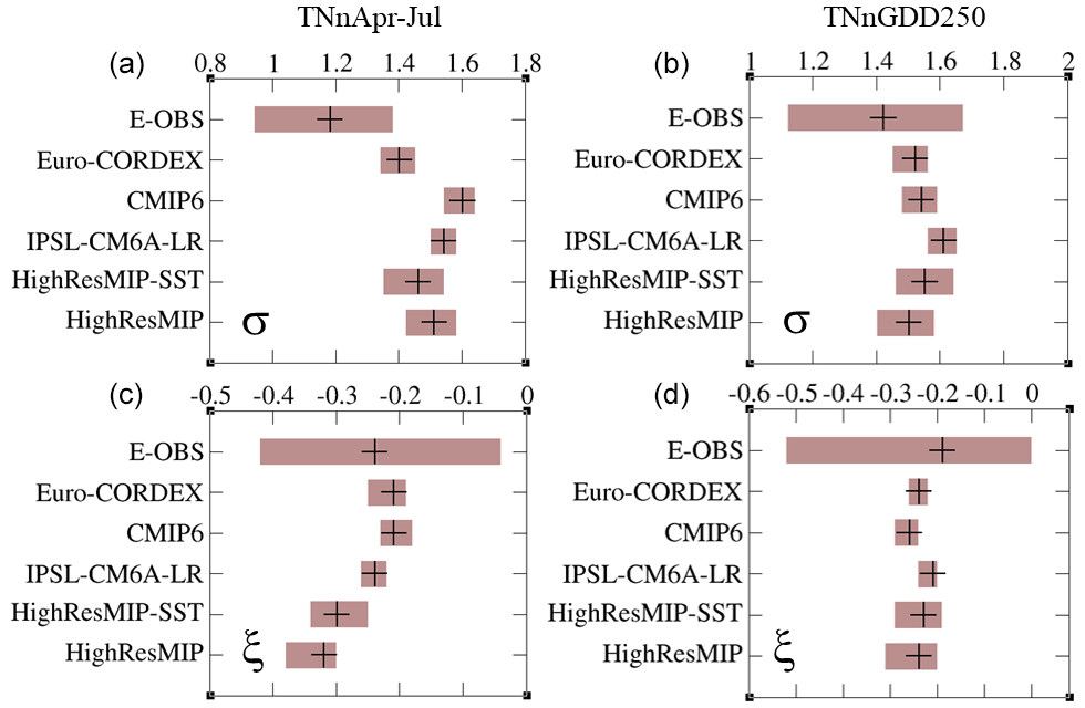
Figure 3Model evaluation, using two main indices, TNnApr–Jul (a, c) and TNnGDD250 (b, d). The estimates of the scale parameters are displayed in the first row and the estimates for the shape parameters in the second row. Results for TNnGDD250-350 are qualitatively similar to those for TNnGDD250.
4.1 Observations
In Fig. 4, we show the annual time series of the indices as obtained from E-OBS, together with simple trend statistics for the 1951–2020 period. The April–July TNn has a slightly upward linear trend of +0.13 ∘C per decade, which is however not significant at the 90 % (two-sided) level because of the large interannual and interdecadal variabilities. By contrast, both TNnGDD250 and TNnGDD250-350 have a significant cooling trend of −0.21 and −0.25 ∘C per decade respectively. The warming trend in TNnApr–Jul is partly due to larger values since 2000, but these higher values are not reflected in the other indices, because GDD has also increased during this period, allowing lower daily minimum temperatures to be counted earlier in the season. We conclude that, on average, since 1950, extreme yearly minimum temperatures for GDD >250 have cooled by about 1.5–2.0 ∘C. Very low growing-period frosts were also found in 1957 and 1991, with lower values than in 2021.

Figure 4(a) Time series of the yearly indices and their respective linear trends calculated over the 1951–2020 period. (b) The same as panel (a) but for TNnGDD250, TNnGDD150 and TNnGDD350.
For different thresholds we also find cooling trends, however with lower significance (Fig. 4b). The significance of the signal remains. Interestingly, over the last 50 years (1971–2020) the trends have increased and have become more significant (for instance +0.29 ∘C per decade, p<0.1 for TNnApr–Jul and −0.37 ∘C per decade for TNnGDD250, p<0.1).
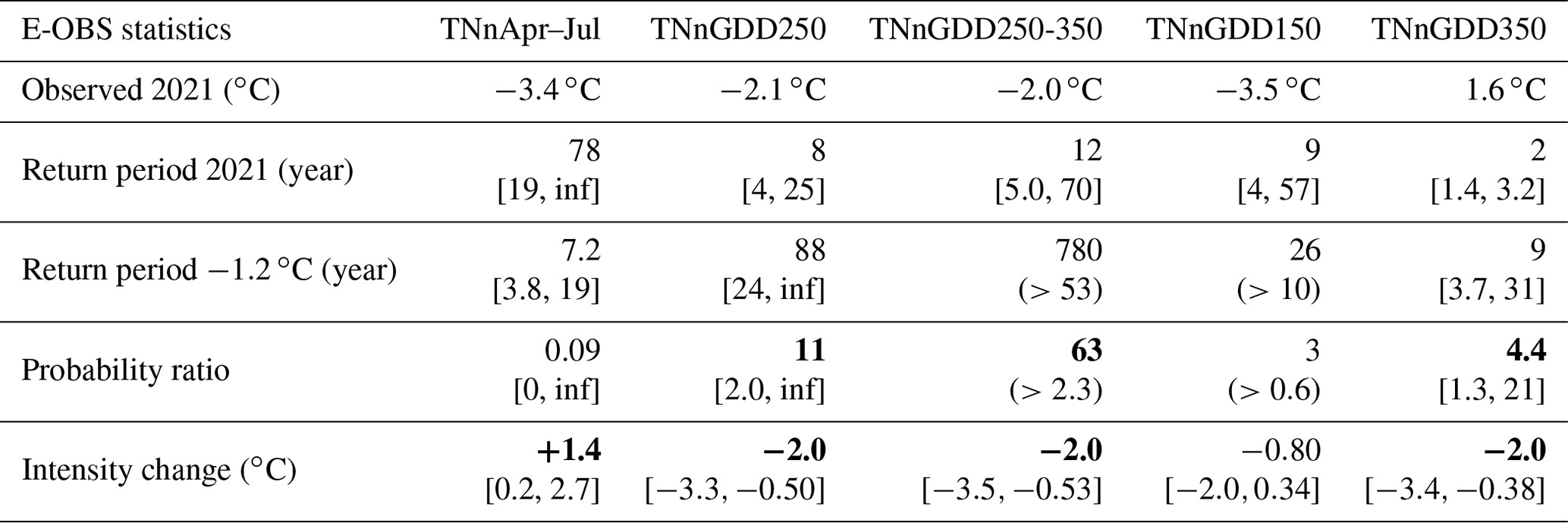
When considering trends in low extremes of these indices, the results are qualitatively similar, but significance is increased when considering GEV fitting using the smoothed observed GMST as covariate instead of assuming a linear trend (see Table 1). We estimate that the event, defined as minimum temperatures over April–July, has a return period of 78 years (at least 19 years), which means a very rare event in the current climate. However, in a climate corresponding to a global temperature 1.2 ∘C cooler, this would have been about a 1-in-7-year event (best estimate). By contrast, the minimum temperature, taken over the growing period as characterized by the GDD index, instead of fixed month, has significantly cooled by almost 2 ∘C with large varying uncertainty ranges and significance depending on the chosen index. The observational analysis is however not sufficient to conclude the role of climate change, which would require models with factual and counterfactual assumptions.
Table 1Extreme value statistics and observations for the various indices and using the 1951–2020 period and a GEV fit with GMST covariate. Bold font denotes statistical significance at the two-sided 95 % level. The observed value of each index is shown in the first row; the calculated return periods from the GEV fit of the yearly data series for 2021 and for the preindustrial climate (assumed to have a global temperature 1.2 ∘C lower than today) are shown in rows no. 2 and no. 3. The probability ratio (the ratio of the return periods) is shown in row no. 4, and the resulting intensity change from the GEV fit is shown in row no. 5 (see Philip et al., 2020 for methodological details).
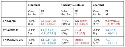
To assess the changes at a local scale, we also calculated trends for three specific stations in the domain (stars in Fig. 2). We selected a subset of three Météo-France reference stations, which were selected in grapevine regions (Beaucouzé: downstream Loire valley; Charnay-les-Mâcon: Burgundy; Charmeil: Saint-Pourçain grapevine), with several characteristics: for Beaucouzé, light frost and non-exceptional event (−1.3 ∘C) but high GDD (321 ∘C d−1 on 5 April); for Charnay-les-Mâcon, record frost (−4.4 ∘C, with 266 ∘C d−1 on 5 April); and for Charmeil, the most severe frost among stations at our disposal (−6.6 ∘C with 244 ∘C d−1 on 5 April). Detection results are shown in Table 2 for these stations and for the three main indices: TNnApr–Jul, TNnGDD250 and TNnGDD250-350. In most cases, the trends are positive for the fixed season index and negative for the growing season period. However, almost no result is statistically significant. We conclude that at a local scale, variability is dominating trend signals (Table 2).
Table 2Return periods, probability ratios (PRs) and changes in intensities (ΔI) obtained from the observations at three stations located as in Fig. 2b. Italics indicate a warming change and bold a cooling change.
Results here differ from the rapid attribution analysis (Vautard et al., 2021) in the completion and adjustment of the E-OBS dataset by the producers. This led to slightly different values for the observed indices in 2021. For instance, the estimation of the TNnGDD250 index-based return period was estimated here to be 8 years instead of 12 years in the rapid attribution. However, the results are qualitatively similar to those found in the preliminary analysis.
4.2 Simulated mean trends
The trends in the two main indices for the five model ensembles are analysed in the form of histograms (Fig. 5), in order to examine the variability across ensemble members. There is a large range of minimum temperature trends from April to July, which are almost all positive. The observed trend in the minimum temperature from April to July is close to the median middle of the distribution for the EURO-CORDEX and the CMIP6 ensemble, while it is closer to the lower tail of the distribution of the remaining three ensembles. A large range of possibilities is also found for the trends of the TNnGDD250 index, with a large part of the simulations showing negative and lower trends than those of the minimum temperature from April to May, consistent with the observations. We conclude from these figures that, despite the general trend towards cooling of the growing-period frosts, the expected trend, for a given singular member, can also be a warming one, albeit with a smaller chance than for a cooling one. This large uncertainty also has to be taken into account in any adaptation strategy.
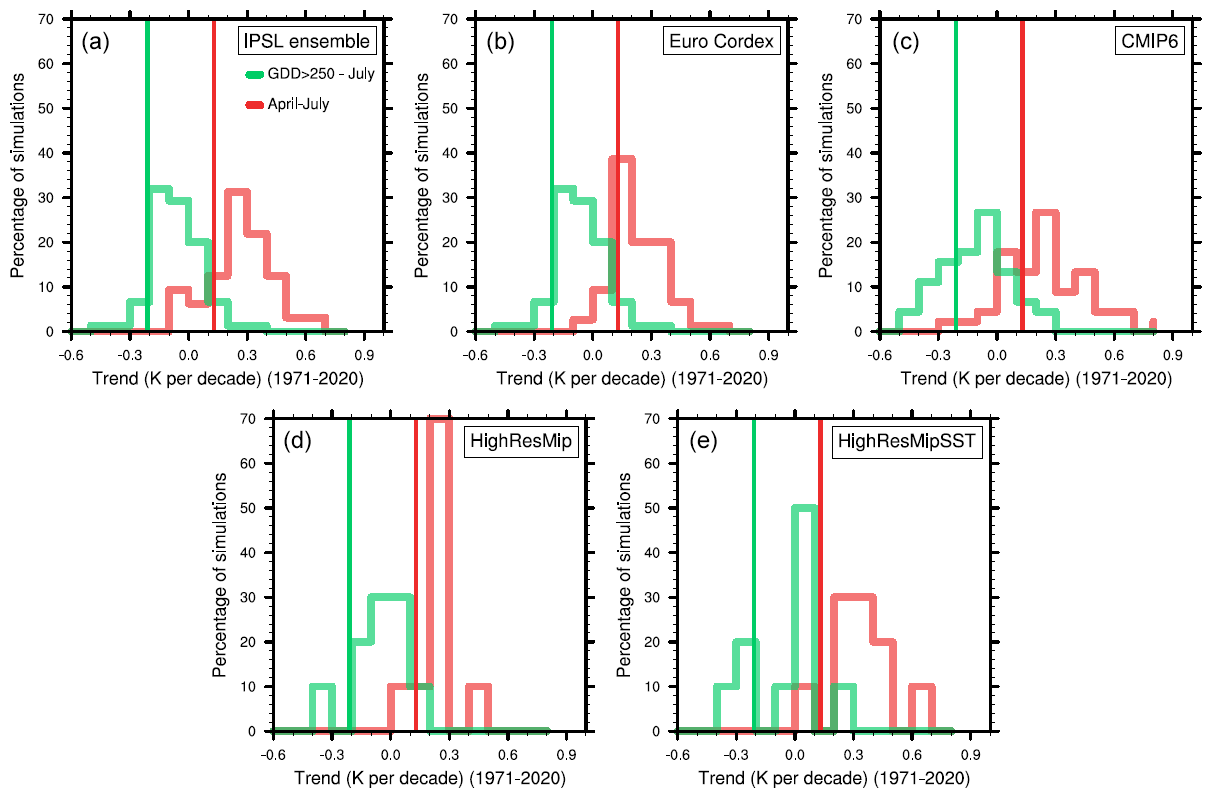
Figure 5Histogram of the daily minimum temperature trend calculated from (a) the IPSL ensemble, (b) the EURO-CORDEX ensemble, (c) the CMIP6 ensemble, (d) the HighResMip ensemble and (e) the HighResMipSST ensemble (see Sect. 4.1 and the Supplement for more details about these ensembles). The observations are represented with the vertical lines. The trends are calculated over the 1971–2020 period for (green) GDD >250 and (red) from April to May.
4.3 Simulated growing-period frost extreme trends and attribution
Figure 6 shows, as an example, the change in return values vs. return periods for indices TNnApr–Jul and TNnGDD250 for the EURO-CORDEX ensemble, and Table 3 shows the extreme value statistics for all indices for this ensemble, as well as other ensembles used. Models show large agreement with observations on changes in return periods and intensities between the preindustrial and current climates for the fixed-calendar TNn index (TNnApr–Jul). The trends in all models seem however underestimated compared to observations for the indices with a GDD conditioning (TNnGDD250).
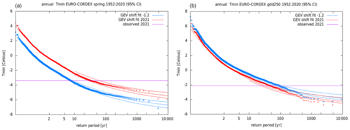
Figure 6Return value vs. return period for EURO-CORDEX and the indices TNnApr–Jul (a) and TNnGDD250 (b) averaged over the study area (the rectangle shown in Fig. 2b). The observed values from E-OBS are marked by the purple line. Note however that the observed values were not the values used to calculate the probability ratio of the event in the EURO-CORDEX ensemble, as the ensemble has a bias toward higher values.
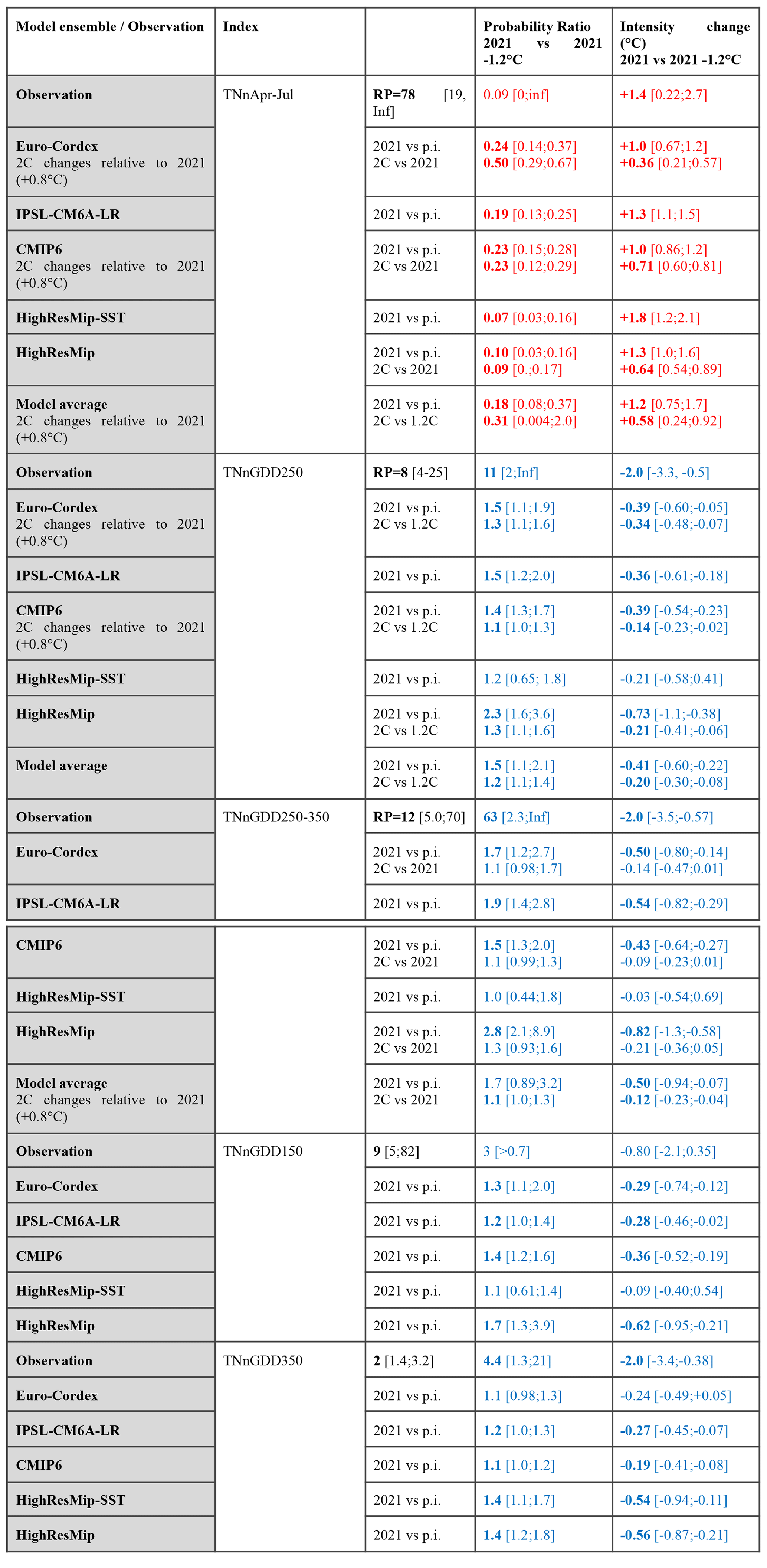
Table 3Change in extreme value statistics for all model ensembles and observations, with the GEV model fitted from data over the 1951–2020 period for the past trend estimates and over the 2000–2050 period for future trends (when estimating the changes for a 2 ∘C warming above preindustrial levels). We assume here that the preindustrial (p.i.) global warming level is 1.2 ∘C cooler than the 2021 one; and therefore, the 2 ∘C warming level is reached when the warming is 0.8 ∘C above the current level. In each row, the values of the probability ratio (the ratio between inverse return periods) are shown, as well as the intensity change, obtained by using the same return period threshold as in the observations, together with their 95 % confidence levels as obtained from a bootstrap estimate using 1000 samples. Numbers in blue indicate a decrease of TN and in red an increase of TN. The last row indicates changes for a 2 ∘C warming level. Boldface numbers indicate statistical significance against a “no change” assumption.
The behaviour present in all model analysis is illustrated in Fig. 6: a clear, significant increase in TNnApr–Jul and an opposite trend sign for TNnGDD250. Despite being weaker, this increasing trend in low extremes is significant for all ensembles but HighResMIP-SST (Table 3), with a clear signal of increase in coldest temperatures when considered over the growing period, and with a threshold of 250 ∘C d−1. Such a trend is also clear and significant in most ensembles when considering the sensitive range where young leaves and flowers are vulnerable to frost. For the other indices, trends are also significant in most cases but not all.
Despite an agreement on the sign between models and observations on trends, models generally simulate much weaker trends for the GDD-conditioned indices than the observed, a fact that remains unexplained, just as the underestimation in extreme temperatures in summer heat waves (see e.g. Vautard et al., 2020; Van Oldenborgh et al., 2022). For TNnGDD250, all ensembles simulate an increase in the frequency of growing-period low extreme temperatures ranging from 10 % to 110 % with a weighted best estimate of 50 % (see also Sect. 5). For the other indices the range of factors is rather similar, despite lower values for TNnGDD350. Changes in intensities are also all negative but remain below 1 ∘C.
4.4 Future trends
Indices have similar future projected trends as in the past few decades in the ensembles and scenarios considered here. Figure 7 shows evolutions of the ensemble median and 10th and 90th percentiles for EURO-CORDEX (RCP8.5) and CMIP6 (SSP3-7.0), for example, but similar results hold for the other ensembles, which have less members or shorter time coverages. In both cases, the median of April–July minimum temperatures over the region continues to increase with mean values around 2 ∘C, while they are below frost level in 2021. By the end of the century, frost such as in 2021 will become a very rare occurrence in April or after in these scenarios. However, frost can still be expected earlier in the year, while at the same time the growing season starts earlier. This can be seen in the development of the TNnGDD250 index throughout the 21st century which shows a weak decreasing trend. It is noteworthy that in the second half of the century, the 10th percentile often nears or exceeds the 2021 value. More frequent events like that in 2021 are therefore expected. By the end of the century for this scenario, we also expect deep frosts in the growing period with intensities which have never been met in 2021 or in earlier years.
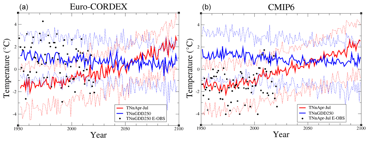
Figure 7Time evolution of the median (thick line) and the 10th and 90th percentiles (dashed lines) of the ensembles EURO-CORDEX (75 members) and CMIP6 (45 members) for the indices TNnApr–Jul (red) and TNnGDD250 (blue). Black dots represent the observations from E-OBS, on panel (a) for EURO-CORDEX, on panel (b) for CMIP6.
Figure 7 also includes the observed time series for the two indices. For TNnGDD250, even though points generally fit well into the 10 %–90 % model range (expected because the models are bias-corrected), we observe a bias in low extremes with variability in the observations inducing frequent excursion in temperatures far below the 10 % quantile. Such bias is not found in the TNnApr–Jul index.
We restrict the analysis of future trends in extremes to the 2 ∘C warming level above the P.I. conditions, which is assumed to be 0.8 ∘C above the current level in 2021. This restriction is made to be on the safe side with potential nonlinearity of response of the extreme indices to global warming, while we assume linearity here with the covariate GEV method. In this future case the GEV fit is carried out over the 2000–2050 period, and probability ratios and intensity changes are given for events with a similar return period as for the 2021 event.
Results are shown along with attribution results in Table 3. Extreme cold temperatures for the April–July period will continue to become less extreme. EURO-CORDEX simulations, which are the only ones consistent with observed trends, project that events similar to the 2021 event would become about half as frequent in a 2 ∘C warming climate. The other models predict factors ranging from between 3 and 10 times less frequent. In contrast, the growing-period extreme frost intensity is increasing, and the 2021 event with a GDD >250 is projected to have an increasing frequency by about 30 % (10 %–60 %) for a 2 ∘C warmer climate than preindustrial in EURO-CORDEX, 10 % (0 %–30 %) for CMIP6 selections and 30 % (10 %–60 %) for HighResMIP (coupled).
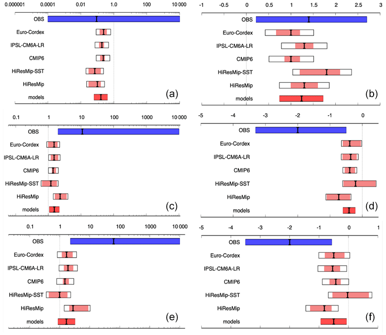
Figure 8Changes between the past and present: summary of observational (blue) and model (red) results for probability ratio (a, c, e, giving the change in the probabilities between the climate with a 1.2 ∘C cooler global temperature and the current climate, as well as change in intensity [∘C] (b, d, f) in the three indices, TNnApr–Jul (a, b), TNnGDD250 (c, d) and TNnGDD250-350 (e, f), as averaged over the study area (see rectangle in Fig. 2b). Extent of the bars gives the two-sided 95 % confidence intervals accounting for internal variability (pink) of each ensemble and model spread added (white), calculated as explained in Philip et al. (2020), with the black marker indicating the best estimate. A weighted average of model results is shown in bright red (label “models”). Note that, for the index TNnApr–Jul, only EURO-CORDEX and HighResMIP-SST passed the validation step, but other models are included in the weighted average for reasons described in the text.
The individual assessments described above for probability ratio and intensity changes in the past period are summarized in Fig. 8. Given the large differences between models and observations for the growing-period indices TNnGDD250 and TNnGDD250-350, we do not combine the observational and model results to form a single “synthesis”, but instead we present the models' weighted average for comparison with the observations. In the case of the TNnApr–Jul index, only two ensembles, EURO-CORDEX and HighResMip-SST, pass the validation criteria. However, the three additional models (IPSL-CM6A-LR, CMIP6 and HighResMip) that validate well for TNnGDD250 and TNnGDD250-350 give similar results to the other ones. Incorporating them in the weighted average has no impact on the high significance of the change found and makes the comparison across indices consistent.
While uncertainties are comparably large for the quantitative assessment of probability ratios, there is a significant decrease in the likelihood of cold waves as defined above for TNnApr–Jul. The event that occurred in 2021, taken as a fixed-season extreme, has become rare, with a return period of at least 19 years and with a best estimate of 78 years. The intensity of a cold wave as observed in April is also decreasing by a well-constrained best estimate of 1.2 ∘C. When considering the lowest temperatures after the growing season start simulated by the GDD thresholds, models and observations quantitatively disagree with respect to probability ratio and intensity, but the qualitative agreement is clear and shows an increase in the likelihood of damaging frost, as well as an increase in the intensity across all indices. This is corroborated by the fact that these trends continue under future warming (see below). This allows for a clear qualitative attribution of these trends to anthropogenic climate change with the model results serving as lower bounds.
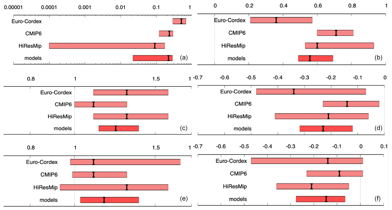
Figure 9Projected changes between the present and +2∘C climate. Summary of results for probability ratio (a, c, e) and change in intensity [∘C] (b, d, f) in the three indices TNnApr–Jul (a, b), TNnGDD250 (c, d) and TNnGDD250-350 (e, f). Extent of the bars gives two-sided 95 % confidence intervals accounting for variability within the datasets, with the black marker indicating the best estimate. A weighted average of the results is shown in bright red.
In Fig. 9 we summarize the projected changes in probability and intensity between the present and +2 ∘C climate, showing an unweighted average for the three model ensembles EURO-CORDEX, CMIP6 and HighResMIP. We again use all available models for TNnApr–Jul despite CMIP6 and HighResMIP ensembles not passing the validation over the historical period. We do so because (i) all models are included for the other two indices, and we do not know how well they validate for the future, and (ii) no synthesis is formed, so the unweighted average shown is only of qualitative use. Probability ratios are less than unity for TNnApr–Jul, indicating that the current trend for decreasing frequency of cold snaps is likely to continue in the future. Projections indicate a decrease by a factor of about 5 in the type of event witnessed in 2021. Likewise, the projections for change in intensity indicate that April–July cold snaps will continue to warm by a best-estimated increase of about 0.6 ∘C. Growing-period minimum temperatures with GDD =250 ∘C d−1 continue to decrease with a best estimate of about 0.2 ∘C and an increase in frequency of about 20 %.
While the growing season is starting earlier, necessary plant dormancy characteristics also change, and the lack of chilling winter days may delay the bud burst in many species (Chuine et al., 2016). This effect is not taken into account here and could alter our results concerning changes in bud burst dates. Such dates are also dependent on species. We have tested the dependence on thresholds of a simple GDD index, which provide similar results than the central thresholds discussed in the synthesis. Dormancy effects, as well as other specific plant effects, can only be studied through impact models, which was not the goal in this study.
The applicability of our results at a local scale is limited in quantitative terms. The local station analysis and the trend histograms show that given locations are more likely to exhibit cooling of extreme growing-period temperatures than warming, but a warming cannot be excluded at these scales and at present-day warming levels.
The discrepancy between trends in models and in observations in the historical periods currently remains unexplained. It shows that either large variability inhibits an accurate estimation of trends of cold extremes or that other factors come into play which may not be well simulated such as trends in radiation or cloudiness as a response to either warming or aerosols. These factors should be investigated in future studies.
Above all, the finding that trends identified up until now continue under future warming indicates that anthropogenic climate change is an important driver of the observed trends and suggests that the models indeed underestimate the effect of change due to forcing factors and that the discrepancy between observed and simulated trends is not entirely explainable by unmodelled factors other than human-induced climate change.
In conclusion, we identify two key attributable effects, the decrease in likelihood and intensity of minimum temperatures and the increase of likelihood and intensity of minimum temperatures when conditioned on growing degree indices. These findings are consistent across the different lines of evidence pursued despite the quantitative differences. The GDD indices are however a crude representation of the vulnerability of different species to frost. Thus, our findings highlight that growing-season frost damage is a potentially extremely costly impact of climate change already damaging the agricultural industry, but to inform adaptation strategies for specific species, impact-based modelling will need to complement our assessment. Other studies, in particular, have indicated that impacts may be highly variable across locations and species (Leolini et al., 2018), emphasizing this need.
All datasets are available from the Climate Explorer at https://climexp.knmi.nl/francespring_timeseries.cgi?id=5f4fa945dc278ae21c3c6df2f705243d (last access: 1 February 2023). The freely available Climate Explorer code was used for the analysis and can be downloaded from Royal Netherlands Meteorological Institute Open Source (https://gitlab.com/KNMI-OSS/climexp?sort=nameasc, last access: 1 February 2023).
The supplement related to this article is available online at: https://doi.org/10.5194/nhess-23-1045-2023-supplement.
RV, GJvO and RB designed the experiments and the related analyses, advised by FO, NV, MR and IGdCA. SL, SK, SP, YR, RB, BD and JMS helped prepare the datasets. All authors contributed to the text.
The contact author has declared that none of the authors has any competing interests.
Publisher's note: Copernicus Publications remains neutral with regard to jurisdictional claims in published maps and institutional affiliations.
We are grateful to James Ciarlo (ICTP) who made one of the regional climate simulations for the EURO-CORDEX ensemble available on ESGF in advance to publication. The analysis benefitted from the collection of the EURO-CORDEX simulations made within the Copernicus Climate Change Service. We acknowledge the E-OBS dataset from the EU-FP6 project UERRA (http://www.uerra.eu, last access: 1 October 2021), the Copernicus Climate Change Service and the data providers in the ECA&D project (https://www.ecad.eu, last access: 1 October 2021).
Our colleague, co-author Geert Jan van Oldenborgh, started the analysis with the authors' team but sadly passed away in October 2021 before the article was submitted. The first author dedicates this study to his mother who passed away the day before the frost event and who gave him her passion for flowers, nature and weather.
This research has been supported by the European Union's Horizon 2020 research and innovation programme (grant no. 101003469, XAIDA project).
This paper was edited by Ricardo Trigo and reviewed by two anonymous referees.
AGRESTE: Bilan conjoncturel 2021, Synthèses conjoncturelles, December 2021, Nb 383, AGRESTE, Ministère de l'Agriculture et de l'Alimentation, https://agreste.agriculture.gouv.fr/agreste-web/download/publication/publie/BilanConj2021/Bilan_conjoncturel_2021_Definitif.pdf last access: 28 February 2023), 2021 (in French).
Barnes, E. A. and Screen, J. A.: The impact of Arctic warming on the midlatitude jet-stream: Can it? Has it? Will it?, WIREs Clim. Change, 6, 277–286, https://doi.org/10.1002/wcc.337, 2015.
Bartók, B., Tobin, I., Vautard, R., Vrac, M., Jin, X., Levavasseur, G., Denvil, S., Dubus, L., Parey, S., Michelangeli, P.-A., Troccoli, A., and Saint-Drenan, Y. M.: A climate projection dataset tailored for the European energy sector. Climate services, 16, 100138, https://doi.org/10.1016/j.cliser.2019.100138, 2019.
Blackport, R., and Screen, J. A.: Insignificant effect of Arctic amplification on the amplitude of midlatitude atmospheric waves, Science Advances, 6, eaay2880, https://doi.org/10.1126/sciadv.aay288, 2020.
Besson, F., Dubuisson, B., Etchevers, P., Gibelin, A.-L., Lassegues, P., Schneider, M., and Vincendon, B.: Climate monitoring and heat and cold waves detection over France using a new spatialization of daily temperature extremes from 1947 to present, Adv. Sci. Res., 16, 149–156, https://doi.org/10.5194/asr-16-149-2019, 2019.
Bonnet, R., Boucher, O., Deshayes, J., Gastineau, G., Hourdin, F., Mignot, J., Servonnat, J., and Swingedouw, D.: Presentation and evaluation of the IPSL-CM6A-LR Ensemble of extended historical simulations, J. Adv. Model. Earth Sy., 13, e2021MS002565, https://doi.org/10.1029/2021MS002565, 2021.
Boucher, O., Servonnat, J., Albright, A. L., Aumont, O., Balkanski, Y., Bastrikov, V., Bekki, S., Bonnet, R., Bony, S., Bopp, L., Braconnot, P., Brockmann, P., Cadule, P., Caubel, A., Cheruy, F., Codron, F., Cozic, A., Cugnet, D., D'Andrea, F., Davini, P., Lavergne, C. de, Denvil, S., Deshayes, J., Devilliers, M., Ducharne, A., Dufresne, J.-L., Dupont, E., Éthé, C., Fairhead, L., Falletti, L., Flavoni, S., Foujols, M.-A., Gardoll, S., Gastineau, G., Ghattas, J., Grandpeix, J.-Y., Guenet, B., Guez, L., Guilyardi, É., Guimberteau, M., Hauglustaine, D., Hourdin, F., Idelkadi, A., Joussaume, S., Kageyama, M., Khodri, M., Krinner, G., Lebas, N., Levavasseur, G., Lévy, C., Li, L., Lott, F., Lurton, T., Luyssaert, S., Madec, G., Madeleine, J.-B., Maignan, F., Marchand, M., Marti, O., Mellul, L., Meurdesoif, Y., Mignot, J., Musat, I., Ottlé, C., Peylin, P., Planton, Y., Polcher, J., Rio, C., Rochetin, N., Rousset, C., Sepulchre, P., Sima, A., Swingedouw, D., Thiéblemont, R., Traore, A. K., Vancoppenolle, M., Vial, J., Vialard, J., Viovy, N., and Vuichard, N.: Presentation and evaluation of the IPSL-CM6A-LR climate model, J. Adv. Model. Earth Sy., 12, e2019MS002010, https://doi.org/10.1029/2019MS002010, 2020.
Chuine, I., Bonhomme, M., Legave, J. M., García de Cortázar-Atauri, I., Charrier, G., Lacointe, A., and Améglio, T.: Can phenological models predict tree phenology accurately in the future? The unrevealed hurdle of endodormancy break, Glob. Change Biol., 22, 3444–3460, 2016.
Climate Explorer: France spring frost study, KNMI, https://climexp.knmi.nl/francespring_timeseries.cgi?id=5f4fa945dc278ae21c3c6df2f705243d (last access: 1 February 2023).
Coppola, E., Nogherotto, R., Ciarlò, J. M., Giorgi, F., van Meijgaard, E., Kadygrov, N., Iles, C., Corre, L., Sandstad, M., Somot, S., Nabat, P., Vautard, R., Levavasseur, G., Schwingshackl, C., Sillmann, J., Kjellström, E., Nikulin, G., Aalbers, E., Lenderink, G., Christensen, O. B., Boberg, F., Sørland, S. L., Demory, M.-E., Bülow, K., Teichmann, C., Warrach-Sagi, K., and Wulfmeyer, V.: Assessment of the European Climate Projections as Simulated by the Large EURO-CORDEX Regional and Global Climate Model Ensemble, J. Geophys. Res.-Atmos., 126, e2019JD032356, https://doi.org/10.1029/2019JD032356, 2021.
Cornes, R. C., van der Schrier, G., van den Besselaar, E. J. M., and Jones, P. D.: An Ensemble Version of the E-OBS Temperature and Precipitation Datasets, J. Geophys. Res.-Atmos., 123, 9391–9409, https://doi.org/10.1029/2017JD028200, 2018.
Eyring, V., Bony, S., Meehl, G. A., Senior, C. A., Stevens, B., Stouffer, R. J., and Taylor, K. E.: Overview of the Coupled Model Intercomparison Project Phase 6 (CMIP6) experimental design and organization, Geosci. Model Dev., 9, 1937–1958, https://doi.org/10.5194/gmd-9-1937-2016, 2016.
García de Cortázar-Atauri, I., Brisson, N., and Gaudillere, J. P.: Performance of several models for predicting budburst date of grapevine (Vitis vinifera L.), Int. J. Biometeorol., 53, 317–326, https://doi.org/10.1007/s00484-009-0217-4, 2009.
Haarsma, R. J., Roberts, M. J., Vidale, P. L., Senior, C. A., Bellucci, A., Bao, Q., Chang, P., Corti, S., Fučkar, N. S., Guemas, V., von Hardenberg, J., Hazeleger, W., Kodama, C., Koenigk, T., Leung, L. R., Lu, J., Luo, J.-J., Mao, J., Mizielinski, M. S., Mizuta, R., Nobre, P., Satoh, M., Scoccimarro, E., Semmler, T., Small, J., and von Storch, J.-S.: High Resolution Model Intercomparison Project (HighResMIP v1.0) for CMIP6, Geosci. Model Dev., 9, 4185–4208, https://doi.org/10.5194/gmd-9-4185-2016, 2016.
IPCC: Climate Change 2021: The Physical Science Basis. Contribution of Working Group I to the Sixth Assessment Report of the, Intergovernmental Panel on Climate Change, edited by: Masson-Delmotte, V., Zhai, P., Pirani, A., Connors, S. L., Péan, C., Berger, S., Caud, N., Chen, Y., Goldfarb, L., Gomis, M. I., Huang, M., Leitzell, K., Lonnoy, E., Matthews, J. B. R., Maycock, T. K., Waterfield, T., Yelekçi, O.,, Yu, R., and Zhou, B., Cambridge University Press, Cambridge, United Kingdom and New York, NY, USA, in press, 2021.
Kew, S. F., Philip, S. Y., van Oldenborgh, G. J., van der Schrier, G., Otto, F. E. L., and Vautard, R.: The Exceptional Summer Heat Wave in Southern Europe 2017, B. Am. Meteorol. Soc., 100, S49–S53, https://doi.org/10.1175/BAMS-D-18-0109.1, 2019.
Leolini, L., Moriondo, M., Fila, G., Costafreda-Aumedes, S., Ferrise, R., and Bindi, M.: Late spring frost impacts on future grapevine distribution in Europe, Field Crop. Res., 222, 197–208, 2018.
Liu, Q., Piao, S., Janssens, I. A., Fu, Y., Peng, S., Lian, X. U., Ciais, P., Myneni, R. B., Peñuelas, J., and Wang, T.: Extension of the growing season increases vegetation exposure to frost, Nat. Commun., 9, 1–8, 2018.
Michelangeli, P. A., Vautard, R., and Legras, B., Weather regimes: Recurrence and quasi stationarity, J. Atmos. Sci., 52, 1237–1256, 1995.
Philip, S., Kew, S. F., van Oldenborgh, G. J., Aalbers, E., Vautard, R., Otto, F., Haustein, K., Habets, F., and Singh, R. : Validation of a rapid attribution of the May/June 2016 flood-inducing precipitation in France to climate change, J. Hydrometeorol., 19, 1881–1898, 2018.
Philip, S., Kew, S., van Oldenborgh, G. J., Otto, F., Vautard, R., van der Wiel, K., King, A., Lott, F., Arrighi, J., Singh, R., and van Aalst, M.: A protocol for probabilistic extreme event attribution analyses, Adv. Stat. Clim. Meteorol. Oceanogr., 6, 177–203, https://doi.org/10.5194/ascmo-6-177-2020, 2020.
Royal Netherlands Meteorological Institute Open Source: Climate Explorer, GitLab, https://gitlab.com/KNMI-OSS/climexp?sort=nameasc, last access: 1 February 2023.
Screen, J. A. and Simmonds, I.: Exploring links between Arctic amplification and mid-latitude weather, Geophys. Res. Lett., 40, 959–964, https://doi.org/10.1002/grl.50174, 2013.
Sgubin, G., Swingedouw, D., Dayon, G., García de Cortázar-Atauri, I., Ollat, N., Pagé, C., and van Leeuwen, C.: The risk of tardive frost damage in French vineyards in a changing climate, Agr. Forest Meteorol., 250–251, 226–242, https://doi.org/10.1016/j.agrformet.2017.12.253, ISSN 0168-1923, 2018.
Shepherd, T. G.: Atmospheric circulation as a source of uncertainty in climate change projections, Nat. Geosci., 7, 703–708, 2014.
Van Oldenborgh, G. J., Mitchell-Larson, E., Vecchi, G. A., De Vries, H., Vautard, R., and Otto, F.: Cold waves are getting milder in the northern midlatitudes, Environ. Res. Lett., 14, 114004, https://doi.org/10.1088/1748-9326/ab4867, 2019.
van Oldenborgh, G. J., Krikken, F., Lewis, S., Leach, N. J., Lehner, F., Saunders, K. R., van Weele, M., Haustein, K., Li, S., Wallom, D., Sparrow, S., Arrighi, J., Singh, R. K., van Aalst, M. K., Philip, S. Y., Vautard, R., and Otto, F. E. L.: Attribution of the Australian bushfire risk to anthropogenic climate change, Nat. Hazards Earth Syst. Sci., 21, 941–960, https://doi.org/10.5194/nhess-21-941-2021, 2021a.
van Oldenborgh, G. J., van der Wiel, K., Kew, S., Philip, S., Otto, F., Vautard, R., King, A., Lott, F., Arrighi, J., Singh, R., and van Aalst, M.: Pathways and pitfalls in extreme event attribution, Climatic Change, 166, 13, https://doi.org/10.1007/s10584-021-03071-7, 2021b.
Van Oldenborgh, G. J., Wehner, M. F., Vautard, R., Otto, F. E., Seneviratne, S. I., Stott, P. A., Hegerl, G. C., Philip, S., and Kew, S. F.: Attributing and projecting heatwaves is hard: We can do better, Earth's Future, 10, e2021EF002271, https://doi.org/10.1029/2021EF002271, 2022.
Vautard, R.: Multiple weather regimes over the North Atlantic: Analysis of precursors and successors, Mon. Weather Rev., 118, 2056–2081, 1990.
Vautard, R., van Aalst, M., Boucher, O., Drouin, A., Haustein, K., Kreienkamp, F., G. J. van Oldenborgh, Otto, F. E. L., Ribes, A., Robin, Y., Schneider, M., Soubeyroux, J.-M., Stott, P., Seneviratne, S. I., Vogel, M., and Wehner, M.: Human contribution to the record-breaking June and July 2019 heatwaves in Western Europe, Environ. Res. Lett., 15, 094077, https://doi.org/10.1088/1748-9326/aba3d4, 2020.
Vautard, R., Kadygrov, N., Iles, C., Boberg, F., Buonomo, E., Bülow, K., Coppola, E., Corre, L., van Meijgaard, E., Nogherotto, R., Sandstad, M., Schwingshackl, C., Somot, S., Aalbers, E., Christensen, O. B., Ciarlo, J. M., Demory, M.-E., Giorgi, F., Jacob, D., Jones, R. G., Keuler, K., Kjellström, E., Lenderink, G., Levavasseur, G., Nikulin, G., Sillmann, J., Solidoro, C., Sørland, S. L., Steger, C., Teichmann, C., Warrach-Sagi, K., and Wulfmeyer, V.: Evaluation of the large EURO-CORDEX regional climate model ensemble, J. Geophys. Res., 126, e2019JD032344, https://doi.org/10.1029/2019JD032344, 2021.
Vrac, M., Noël, T., and Vautard, R. : Bias correction of precipitation through Singularity Stochastic Removal: Because occurrences matter, J. Geophys. Res.-Atmos., 121, 5237–5258, 2016.