Collective risk modelling of multi-peril events: correlation of European windstorm gust and precipitation annual severity

Hazards such as storms can create multiple perils, such as windstorms and floods, that have correlated annual losses. To better understand the drivers of such correlations, this study explores three collective risk frameworks with varying complexity.

Mathematical expressions are derived explaining how this correlation depends on parameters such as event dispersion (clustering), and the joint distribution of the two hazard variables. Hazard variables are first assumed independent, inducing a positive correlation due to the shared positive dependence on the total number of events. The next framework allows for correlation between the hazard variables, which can then capture negative correlation between accumulated losses. The final framework builds on this by allowing for between-year correlation caused by interannual modulation of the hazard variables.

These frameworks are illustrated using European windstorm gust speeds and precipitation reanalyses from 1980–2000. They are used to diagnose why the correlation between annual wind and precipitation severity indices decreases as thresholds are increased. Only the framework with interannual modulation of the hazard variables quantitatively captures the negative correlations over Europe at high thresholds. We propose that one plausible driver for the modulation is the transit time that storms spend near locations.

1 Introduction

Environmental hazards can often lead to co-occurring perils. For example, extratropical cyclones can lead to losses from co-occurring extreme wind gusts and floods (Raveh‐Rubin and Wernli, 2015; Martius et al., 2016; Owen et al., 2021) as well as from storm surges (Kendon and McCarthy, 2015). Such events are also referred to as multivariate events since the losses result from extremes in multiple hazard variables (Zscheischler et al., 2020). Other examples include high temperatures and low precipitation leading to wildfire in south Australia (Richardson et al., 2022); storm surge and high precipitation leading to flooding after hurricanes (Juárez et al., 2022) and the combined effect of a co-occurring heatwave and drought in Africa and Asia (Wang et al., 2023). The impact from these multi-peril events is often greater than from the sum of impacts from the hazards separately (Hillier and Dixon, 2020).

Multivariate compound weather hazards are receiving increasing attention in studies using a variety of statistical methods. Examples include copulas (Manning et al., 2024); comparing co-occurrence relative to a bootstrapped event set (Hillier et al., 2025), or use of extremal dependency measures (Zscheischler et al., 2021; Owen et al., 2021). These methods generally aim to quantify the dependence between hazard variables of individual events rather than diagnose the drivers of such dependence (Hillier et al., 2020; Bevacqua et al., 2021).

In addition to the individual risk of loss due to single events, it is important for risk managers to also understand the collective risk due to a set of events over the time period that is insured. The annual aggregation over the calendar year from January to December is particularly relevant to the insurance industry as it aligns with typical reinsurance contract timelines (Čížek, 2005). Collective risk not only depends on the individual risk for each event but also on properties such as temporal clustering of the events (Mailier et al., 2006; Vitolo et al., 2009; Hunter et al., 2015). Despite increasing numbers of studies on clustering, much less research has been published on the collective risk of multivariate hazards. It is common practice in insurance to model perils separately and then assume that annual losses from different perils are independent. For example, yearly losses from wind and flood in Europe are modelled separately and then assumed to be uncorrelated (Hadzilacos et al., 2021).

To better understand the correlation between accumulated losses from different perils, this study explores and tests various collective risk modelling frameworks for diagnosing the drivers of such correlation. The methods are demonstrated by applying them to annually aggregated wind and precipitation severities caused by extratropical cyclones over the North Atlantic and Europe from 1980–2020. In particular, we use the frameworks to diagnose the negative correlation noted between annual wind and precipitation severities that was recently presented in Jones et al. (2024).

Damage from both extreme wind and precipitation can occur within the same season (Kendon and McCarthy, 2015). As such the annual cost of extratropical cyclone damage in Europe often reaches billions of Euros (Cusack, 2023). Consequently, protection against wind damage constitutes over 15 % of global reinsurance purchases (Mitchell-Wallace et al., 2017), while the UK needed a not-for-profit flood re-insurance scheme to keep consumer premiums affordable (Browning, 2020). As large loss events are more likely to cluster (Vitolo et al., 2009; Priestley et al., 2018; Renggli and Zimerli, 2016), understanding the relationship between annual wind and precipitation hazards from extratropical cyclones is crucial for re-insurers to best diversify their risk across hazards (Grossi and Kunreuther, 2005; Klugman et al., 2019).

Hillier and Dixon (2020) found a positive relationship between seasonally aggregated extreme wind gusts and precipitation, the wind hazard increases during the wettest years for most of Europe. Almost triple the magnitude of aggregate extreme wind severity (cubed exceedances above 20 m s⁻¹) was occurs between the wettest and driest third of seasons. Similarly, positive correlation was found to exist between wind and precipitation aggregated across the UK from daily to seasonal timescales (Bloomfield et al., 2023). This used Spearman's rank correlation, which is less sensitive to extreme outlier values. However, when using Pearson's correlation, Jones et al. (2024) found that the positive correlation between annual wind and precipitation severities decreased and even became slightly negative over Europe for more extreme severities as thresholds for the hazard variables were increased. Both Hillier and Dixon (2020) and Bloomfield et al. (2023) used the extended winter (October–March) season, while Jones et al. (2024) uses the full calendar year, splitting winters in two.

This study aims to answer the following questions:

• What assumptions are required for a collective risk model to be able to capture the correlation between aggregate losses at all spatial locations?

• Can such a collective risk model quantitatively account for how the correlation changes for more extreme events?

• What are the key drivers of the changes in correlation with threshold?

Section 2 presents three collective risk models of increasing complexity and shows how the correlation of aggregate losses depends on parameters such as overdispersion (clustering), skewness of the hazard variables, and correlation between the individual hazard variables. Section 3 then applies and tests the frameworks on the storm data used in Jones et al. (2024). Conclusions and ideas for future work are presented in Sect. 4.

2 Collective risk modelling

2.1 Severity Indices

The damage or loss at a given location is often approximated to be a function of the hazard variable, i.e. g(X) where X is the hazard variable (e.g. wind gust speed). Idealised forms of these functions are known as Severity Indices (SI). Numerous SIs have been created for wind damage. Klawa and Ulbrich (2003) use the cube of wind gust above the local 98th percentile, with numerous other studies (e.g. Leckebusch et al., 2007, 2008; Pinto et al., 2012; Little et al., 2023) using an SI of similar form adapted to gridded data. Heneka and Ruck (2008) presented an SI using the square of exceedances, although this assumed the damage threshold was normally distributed. Bloomfield et al. (2023) introduced a flood severity index, also using the exceedance over threshold approach, using linear exceedances of river flow data. SIs of this form are less influenced by outlier extreme events. This study uses a simple exceedance over threshold SI defined a

$$\begin{array}{}\text{(1)}& g\left(X\right)=\left\{\begin{array}{ll}X-u_X& X_i>u_X\\ \mathrm{0}& X_i\le u_X.\end{array}\right.\end{array}$$

The threshold u_X can be a fixed value for all locations (e.g. 20 m s⁻¹; Jones et al., 2024) or a percentile of X that varies with location (e.g. u_X = X_0.98; Klawa and Ulbrich, 2003). Klawa and Ulbrich (2003) were one of the first to use this threshold approach, noting German insurers usually pay for damages if a nearby weather station records gusts above 20 m s⁻¹. This approach has since been used in many subsequent studies and has been sensitivity tested (Hillier and Dixon, 2020; Little et al., 2023; Leckebusch et al., 2007; Pinto et al., 2012).

2.2 Aggregate Severity Indices

Accumulated losses over a given time period (e.g. a year) are then approximated by the random sum of Severity Indices g(X_i) over the set of events i = $\mathrm{1},\mathrm{2},\mathrm{\dots },N$ that occurred in the period. Aggregated Severity Indices (ASIs) are frequently used as a proxy for total damage. Correlation between ASIs can therefore be usefully translated into impact on joint financial risk (Hillier et al., 2024). Hillier and Dixon (2020) aggregated wind gust and total precipitation over the extended winter season (October–March), concluding that extreme precipitation winters results in an uplift of aggregate extreme wind hazard for most of Europe. This compared the relative value of wind ASIs for the top and bottom thirds of winters ranked by precipitation ASI. Hunter et al. (2015) used ASIs to investigate the relationship between frequency and mean intensity of windstorms, concluding the Scandinavian Pattern was a driver of this relationship. Jones (2022) derived a framework to model the relationship between frequency and wind ASI, while Jones et al. (2024) found most of Europe have negative Pearson's correlation between wind and precipitation ASIs at high thresholds. From our SI Eq. (1), the ASI is defined as

$$\begin{array}{}\text{(2)}& S_X=\left\{\begin{array}{ll}g\left(X_{\mathrm{1}}\right)+g\left(X_{\mathrm{2}}\right)+\mathrm{\dots }+g\left(X_N\right)& N>\mathrm{0}\\ \mathrm{0}& N=\mathrm{0}.\end{array}\right.\end{array}$$

where $\mathit{\{}{X}_{\mathrm{1}},\mathrm{\dots },X_N\mathit{\}}$ are the hazard variables for each of the N events. The distribution of S_X determines the collective risk of accumulated losses over the chosen time period.

In this study, we shall consider events that have perils caused by two hazard variables X and Y with thresholds u_X and u_Y, respectively, resulting in annual ASI S_X and S_Y. The total number of events, N, only includes events that increase S_X or S_Y (or both) i.e. events where X > u_X or Y > u_Y. This avoids having to model the bivariate distribution of separate counts for extremes in wind and precipitation. The count variable used in this study is an upper bound for these separate counts. For simplicity of notation, we shall refer to X^′ = g(X) and Y^′ = g(Y) simply as X and Y, respectively.

2.3 ASI modelling frameworks

An ASI is the sum of a random number N of random variables $\mathit{\{}{X}_{\mathrm{1}},X_{\mathrm{2}},\mathrm{\dots },X_N\mathit{\}}$ and is known as a random sum in actuarial science (Ambagaspitiya, 1999; Ren, 2012; Tang, 2001). Its distributional properties depend on the distribution of N, the distribution of the X variables, and the joint distribution between N and the X. For example, the expectation (E[S_X]) and variance (Var(S_X)) of random sums have been derived long ago (Wald, 1945; Blackwell and Girshick, 1947). These results assume that the X variables are independent of N, but this assumption can be relaxed (Cohen, 2019).

Far less attention has been given to correlations between random sums. Mirzai (1999) used a simplified approach relying on counts of extremes, although counts were restricted to follow a Poisson distribution (something uncharacteristic of European windstorms, Mailier et al., 2006). Kolev and Paiva (2008) defined a more flexible framework, but this includes S_X and S_Y as explanatory variables. Neither study applied their respective frameworks to real-world hazards. Only Jones (2022) has applied a similar correlation framework to model hazard data, but this focused on frequency and aggregate wind hazard.

This study considers 3 frameworks of increasing complexity. The distinction between the frameworks are their choice of independence assumptions:

• Frequency-Severity Independence (FS-Ind): the severity of hazards within a year are independent to the frequency of events (e.g. storm counts and gust speeds for a year have zero correlation).

• Hazard Independence (H-Ind): the wind and precipitation SIs from the same event are assumed independent (so have zero correlation).

• Serial Independence (S-Ind): hazard SIs from different events are assumed independent (wind values from separate events have zero correlation with each other).

For simplicity, all the frameworks assume FS-Ind, i.e., Cov(N,X_i) = 0 and Cov(N,Y_i) = 0 for $i\in \mathit{\{}\mathrm{1},\mathrm{2},\mathrm{\dots },N\mathit{\}}$. The three frameworks are:

• Framework A: uncorrelated hazard variables [FS-Ind, H-Ind and S-Ind].
  Assumes Cov(X_i,Y_j) = 0 (H-Ind), Cov$(X_i,X_j)={\mathit{\sigma }}_X^{\mathrm{2}}{\mathit{\delta }}_{ij}$ (S-Ind) and Cov$(Y_i,Y_j)={\mathit{\sigma }}_Y^{\mathrm{2}}{\mathit{\delta }}_{ij}$ (S-Ind) for all combinations of $i,j\in \mathit{\{}\mathrm{1},\mathrm{2}\mathrm{\dots },N\mathit{\}}$. As indices i and j take any value from 1 to N, dependency between all hazard pairs within a year is considered. Most hazard pairs have zero covariance as δ_ij = 1 if i = j and is 0 otherwise. The standard deviations for hazards X and Y are σ_X and σ_Y. These are common assumptions often used by actuaries (Kaas et al., 2008).

• Framework B: correlated hazard variables.
  Assumes Cov$(X_i,Y_j)=\mathit{\theta }{\mathit{\sigma }}_X{\mathit{\sigma }}_Y{\mathit{\delta }}_{ij}$, Cov$(X_i,X_j)={\mathit{\sigma }}_X^{\mathrm{2}}{\mathit{\delta }}_{ij}$ (S-Ind) and Cov$(Y_i,Y_j)={\mathit{\sigma }}_Y^{\mathrm{2}}{\mathit{\delta }}_{ij}$ (S-Ind) for all $i,j\in \mathit{\{}\mathrm{1},\mathrm{2}\mathrm{\dots },N\mathit{\}}$. Pearson's correlation θ = Cor$(X_i,Y_i)\in [-\mathrm{1},\mathrm{1}]$ is the correlation between the hazard variables for each event computed over all hazard pairs at each gridpoint. This framework does not assume H-Ind.

• Framework C: correlated hazard variables modulated by Z.
  Assumes Cov$(X_i,Y_j)=\mathit{\theta }{\mathit{\sigma }}_X{\mathit{\sigma }}_Y{\mathit{\delta }}_{ij}+$ Cov$(\stackrel{\mathrm{‾}}{X},\stackrel{\mathrm{‾}}{Y})$, Cov$(X_i,X_j)={\mathit{\sigma }}_X^{\mathrm{2}}{\mathit{\delta }}_{ij}+$ Var$\left(\stackrel{\mathrm{‾}}{X}\right)$ and Cov$(Y_i,Y_j)={\mathit{\sigma }}_Y^{\mathrm{2}}{\mathit{\delta }}_{ij}+$ Var$\left(\stackrel{\mathrm{‾}}{Y}\right)$ for all $i,j\in \mathit{\{}\mathrm{1},\mathrm{2}\mathrm{\dots },N\mathit{\}}$ where $\stackrel{\mathrm{‾}}{X}$ = E(X|Z) and $\stackrel{\mathrm{‾}}{Y}$ = E(Y|Z). Variable Z is a latent variable that is considered to vary between but not within years and can influence X and Y differently. This framework does not assume H-Ind or S-Ind.

The dependency structure of each framework is summarised in Fig. 1. Framework B is a special case of framework C having Var(Z) = 0 (i.e. no interannual modulation), and framework A is a special case of framework B having θ = 0 (i.e. no hazard correlation).

Figure 1 Dependence assumptions for the three frameworks. Arrows show which variables can causally influence others.

Using these assumptions it is possible to derive the Pearson's correlation ρ = Cor(S_X,S_Y) between the aggregate severities for each of the three frameworks (see Appendix A). For framework A, one obtains

$$\begin{array}{}\text{(3)}& {\mathit{\rho }}_A={\displaystyle \frac{\mathit{\varphi }{J}_X{J}_Y}{\sqrt{(\mathrm{1}+\mathit{\varphi }{J}_X^{\mathrm{2}})(\mathrm{1}+\mathit{\varphi }{J}_Y^{\mathrm{2}})}}},\end{array}$$

where ϕ = Var$\left(N\right)/\text{E}\left[N\right]$ is the dispersion in counts (Mailier et al., 2006), and $J_X=\text{E}\left[X\right]/\sqrt{\text{Var}\left(X\right)}$ and $J_Y=\text{E}\left[Y\right]/\sqrt{\text{Var}\left(Y\right)}$ are the signal-to-noise ratios of the two hazard variables. The correlation of framework A is always non-negative and increases from 0 to 1 as the dispersion ϕ goes from 0 to ∞, and hence large amounts of clustering ϕ ≫ 1 induce high correlation between the aggregated severities of the two perils. Framework B gives

$$\begin{array}{}\text{(4)}& {\mathit{\rho }}_B={\displaystyle \frac{\mathit{\theta }+\mathit{\varphi }{J}_X{J}_Y}{\sqrt{(\mathrm{1}+\mathit{\varphi }{J}_X^{\mathrm{2}})(\mathrm{1}+\mathit{\varphi }{J}_Y^{\mathrm{2}})}}},\end{array}$$

where θ = Cor(X_i,Y_i) is the correlation between hazard variables for individual events. Unlike framework A, framework B can produce negative correlations provided θ<ϕJ_XJ_Y. It should be noted that ρ≥θ when θ<0 and so ρ can never be more negative than θ. Framework C gives

$$\begin{array}{}\text{(5)}& \begin{array}{rl}{\mathit{\rho }}_C& ={\displaystyle \frac{\mathit{\theta }+\mathit{\varphi }{J}_{XY}+\mathit{\lambda }{K}_{XY}}{\sqrt{(\mathrm{1}+\mathit{\varphi }{J}_X^{\mathrm{2}}+\mathit{\lambda }{K}_X^{\mathrm{2}})(\mathrm{1}+\mathit{\varphi }{J}_Y^{\mathrm{2}}+\mathit{\lambda }{K}_Y^{\mathrm{2}})}}}\\ & ={\displaystyle \frac{\mathit{\theta }}{\sqrt{d}}}+{\displaystyle \frac{\mathit{\varphi }{J}_{XY}}{\sqrt{d}}}+{\displaystyle \frac{\mathit{\lambda }{K}_{XY}}{\sqrt{d}}},\end{array}\end{array}$$

where λ = E[N], $d=\sqrt{(\mathrm{1}+\mathit{\varphi }{J}_X^{\mathrm{2}}+\mathit{\lambda }{K}_X^{\mathrm{2}})(\mathrm{1}+\mathit{\varphi }{J}_Y^{\mathrm{2}}+\mathit{\lambda }{K}_Y^{\mathrm{2}})}$, θ = $\frac{\text{E}\left[\text{Cov}\right(X\mathrm{|}Z,Y\mathrm{|}Z\left)\right]}{\sqrt{E_Z\left[\text{Var}\right(X\left|Z\right)\text{Var}\left(Y\right|Z\left)\right]}}$ and

$$\begin{array}{ll}{J}_{XY}=\frac{E_Z\left[\text{E}\right[X\left|Z\right]\text{E}\left[Y\right|Z\left]\right]}{\sqrt{E_Z\left[\text{Var}\right(X\left|Z\right)\text{Var}\left(Y\right|Z\left)\right]}}& K_{XY}=\frac{\text{Cov}\left(\text{E}\right[X\left|Z\right],\text{E}\left[Y\right|Z\left]\right)}{\sqrt{E_Z\left[\text{Var}\right(X\left|Z\right)\text{Var}\left(Y\right|Z\left)\right]}}\\ J_X^{\mathrm{2}}=\frac{E_Z\left[\text{E}\right[X\left|Z{]}^{\mathrm{2}}\right]}{E_Z\left[\text{Var}\right(X\left|Z\right)]}& J_Y^{\mathrm{2}}=\frac{E_Z\left[\text{E}\right[Y\left|Z{]}^{\mathrm{2}}\right]}{E_Z\left[\text{Var}\right(Y\left|Z\right)]}\\ K_X^{\mathrm{2}}=\frac{\text{Var}\left(\text{E}\right[X\left|Z\right])}{E_Z\left[\text{Var}\right(X\left|Z\right)]}& K_Y^{\mathrm{2}}=\frac{\text{Var}\left(\text{E}\right[Y\left|Z\right])}{E_Z\left[\text{Var}\right(Y\left|Z\right)]}.\end{array}$$

Physical explanation of these three components is provided in Sect. 3.3. The variable Z is a latent variable that is considered to vary with the years and so then E[X|Z] are the annual means of X, and Cov$\left(\text{E}\right[X\left|Z\right],\text{E}\left[Y\right|Z\left]\right)$ is the covariance between the annual means of X and Y. This framework has the advantage that the interannual modulation can allow ρ to be more negative than θ.

3 Data example: correlation of wind and precipitation storm severity indices

3.1 Storm data 1980–2020

The frameworks in this study are applied to the same data and cyclone extraction procedures as detailed in Jones et al. (2024). The cyclones and hazard variables are extracted from 1-hourly ERA5 reanalysis at the native 0.25° spatial resolution from 1980–2020 (Hersbach et al., 2020). Using hourly data is important for modelling sub-daily rainfall extremes (Whitford et al., 2023).

Cyclones are first identified and tracked at 850 hPa using the TRACK algorithm (Hodges, 1994). This is a widely adopted method for cyclone tracking (Hawcroft et al., 2012; Manning et al., 2023; Priestley and Catto, 2022; Maddison et al., 2020; Yu et al., 2023; Hay et al., 2023) and performs similarly to other tracking algorithms (Bourdin et al., 2022). A constant 5° radius is applied around the tracks to determine the influence of the cyclone, which is comparable to what has been used in previous studies (Hawcroft et al., 2015; Kodama et al., 2019).

Wind and precipitation values are created at each grid point for each cyclone using the maximum 3 s wind gust speeds (x_i) and total accumulated precipitation (y_i) over the duration that each cyclone was within 5° of that grid point. Severity indices are created using Eq. (1) by applying thresholds to these event metrics. Annual ASIs S_X and S_Y were then created for every grid point and every calendar year (1 January–31 December) using Eq. (2).

3.2 Framework skill at modelling correlation

Jones et al. (2024) describes how sample correlation between wind and precipitation ASIs decreases with increasing thresholds, including differing behaviours between regions. This study uses the same fixed thresholds to reproduce the sample Pearsons correlations from Jones et al. (2024), equivalent percentile thresholds are shown in Appendix B (Fig. B1). The correlation between ASIs is not necessarily a result of the correlation between individual wind and precipitation severities, shared positive dependence on event clustering could cancel this out. Frameworks are therefore needed to understand the resulting correlation between ASIs. Figure 2a–c reproduce the sample correlation values at each grid point between wind and precipitation ASIs for different threshold levels shown in Jones et al. (2024). Strong positive correlation occurs across almost all of the domain when thresholds are zero (Fig. 2a). Correlations then reduce for higher thresholds, with regions of negative correlation appearing mostly over land (Fig. 2b). At the highest thresholds, negative correlation becomes more widespread across land and starts to appear in isolated locations in the Atlantic Ocean (Fig. 2c). This land-sea contrast is primarily caused by wind speeds being generally greater over sea (reduced surface roughness). Exceedances over a fixed threshold over sea are therefore less in the extreme tail of the distribution than those over land.

Figure 2 Sample correlation between S_X and S_Y (a–c) and estimates of the correlation from framework A (d–f), framework B (g–i), and framework C (j–l). Columns represent different threshold combinations for (u_X,u_Y): no thresholds (0 m s⁻¹, 0 mm) (a, d, g, j), (10 m s⁻¹, 10 mm) (b, e, h, k) and high thresholds (20 m s⁻¹, 20 mm) (c, f, i, l). The statistical significance of sample correlation is shown in Fig. B3.

A difference in approaches means the relationships in this study (and Jones et al., 2024) are inconsistent with existing wind-precipitation research. This study uses aggregate scores while Martius et al. (2016) and Owen et al. (2021) consider daily co-occurence. Aggregation is computed over the calendar year rather than seasons like Hillier and Dixon (2020). This study also links wind and precipitation to tracked cyclones while Martius et al. (2016) and Hillier and Dixon (2020) use daily data.

It is of interest to see how well the frameworks capture these correlations at different thresholds. Correlations calculated using these frameworks are shown in the panels below: Fig. 2d–f (framework A), Fig. 2g–i (framework B), and Fig. 2j–l (framework C). All the frameworks perform similarly well at capturing the positive correlation when the thresholds are zero (Fig. 2d, g, and j). Framework A shows a decrease in correlation at higher thresholds (Fig. 2e and f), but is unable to produce any of the negative correlations seen in the sample correlations (Fig. 2b and c). Framework B shows greater decrease at higher threshold (Fig. 2h and i) with some small negative correlations appearing but still not as negative as in the sample correlations. Framework C shows a stronger decrease (Fig. 2k and l) with much more extensive negative correlations over land at the highest threshold. The spatial structure of negative correlation over the northwest of mainland Europe is broadly reproduced at the highest thresholds (Fig. 2k). In summary, Framework C is the only framework able to capture the correlations at each of the thresholds.

3.3 Analysis of components in Framework C

The correlation in Eq. (5) is the sum of 3 components each having the same denominator d. The terms can be interpreted as follows:

• Within-year dependency: θ, the “average” of yearly wind-precipitation correlation, computed between hazard pairs occurring from the same storm.

• Event dispersion: ϕJ_XY, the positive dependence induced in S_X and S_Y by their positive relationships with counts. Larger dispersion (ϕ) in annual counts leads to a greater effect.

• Interannual dependency: λK_XY, the relationship between yearly mean values of wind and precipitation, scaled by the mean number of events per year (λ).

Figure 3 shows the decomposition of the correlation ρ for framework C. The event dispersion component is positive at the lowest threshold but decreases towards zero for higher thresholds (Fig. 3g–i). It is the main contributor to ρ at low thresholds as can be seen in the similarity between panels (g) and (a) in Fig. 3. The within-year dependency component is also positive at the lowest threshold (Fig. 3d), but decreases to negative over Europe at the highest threshold (Fig. 3f). The interannual dependency component follows a similar pattern but with a stronger decrease to more negative values at high values of threshold (Fig. 3j–l). The interannual dependency component is the main contributor to ρ at high thresholds as can be seen in the similarity between panels (l) and (l) in Fig. 3.

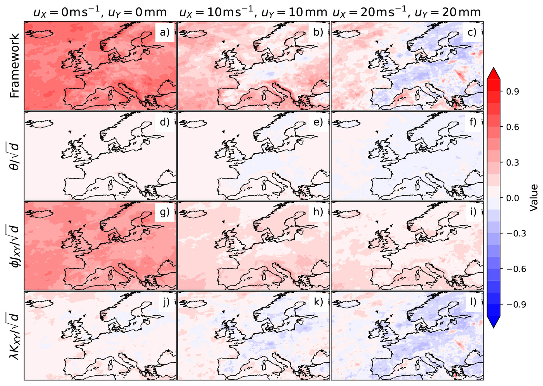
Figure 3 Decomposition of the correlation for framework C: the framework correlation ρ (a–c), $\mathit{\varphi }{J}_{XY}/\sqrt{d}$ (d–f), $\mathit{\theta }/\sqrt{d}$ (g–i), $\mathit{\lambda }{K}_{XY}/\sqrt{d}$ (j–i). Columns represent different threshold combinations for (u_X,u_Y): no thresholds (0 m s⁻¹, 0 mm) (a, d, g, j), (10 m s⁻¹, 10 mm) (b, e, h, k) and high thresholds (20 m s⁻¹, 20 mm) (c, f, i, l).

For more detail on how each of the components varies with threshold, Fig. 4 shows the components versus threshold for a region covering France (red box Fig. 5b). The threshold is set to the same value for both wind and precipitation. For each storm, the SI for the region is calculated by summing the SI from all land and sea grid points in [4.75° W–8.5° E, 42.25–51.75° N]. For a given storm most gridpoint SIs within the region are zero, being > 5° from the storm track or below the threshold. The number of storms is calculated for the entire region by counting the number of events when SI is positive at one or more of the grid points. Correlation, ρ, decreases with increasing threshold and goes negative above 18 m s⁻¹ and 18 mm (red line Fig. 4). This behaviour is generally well captured by the framework (blue dashed line) which mostly falls within the 95 % confidence interval (pink shaded area). The positive event dispersion component (solid thin line) is largely compensated at all thresholds by the negative within-year dependency component (thin dashed line). This results in the framework correlation closely following the interannual dependency component (thin dotted line).

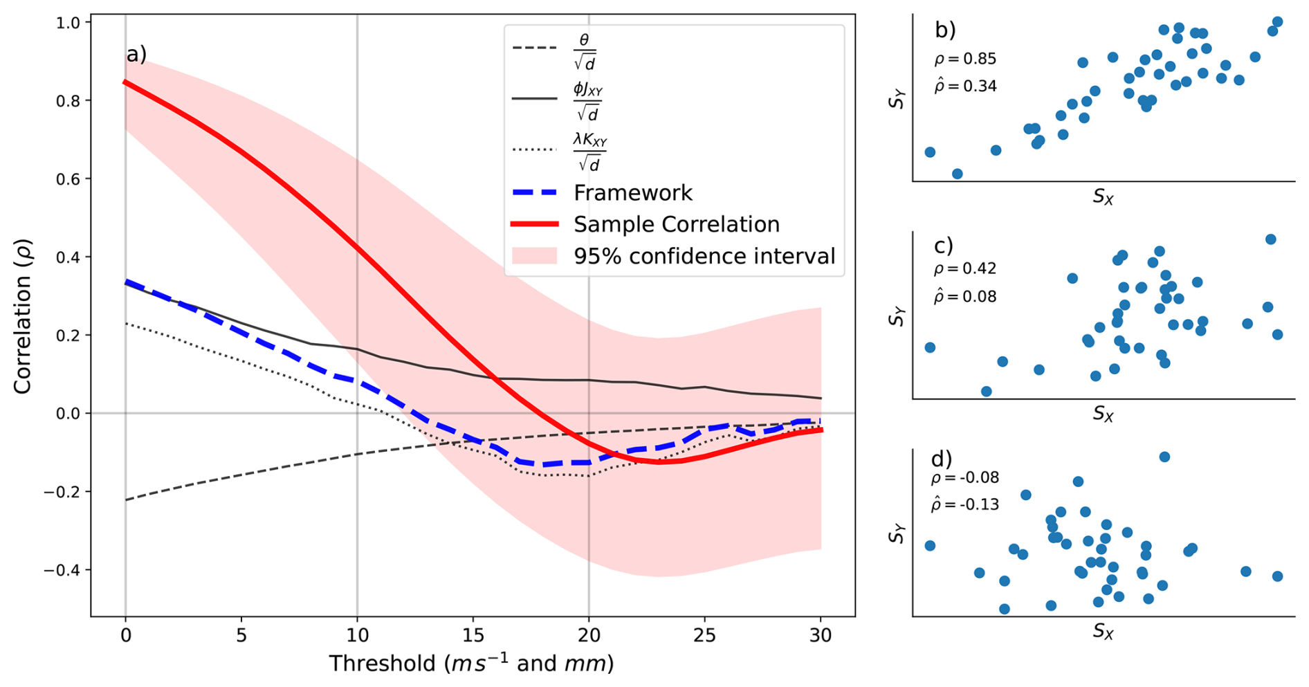
Figure 4 Panel (a) shows Framework C correlation and its components for France (red box in Fig. 5) over a range of threshold levels where u_X = u_Y. Thick lines represent sample correlation (red solid line) and framework estimate (blue dashed line). Thinner lines are each component of the framework: $\mathit{\theta }/\sqrt{d}$ (thin solid line), $\mathit{\varphi }{J}_{XY}/\sqrt{d}$ (thin dashed line), $\mathit{\lambda }{K}_{XY}/\sqrt{d}$ (thin dotted line). Panels (b), (c), (d) show the ASI values and their correlations are the sample pairs shown in bold for threshold combinations (shown by grey vertical lines in panel a) (0 m s⁻¹, 0 mm) (b), (10 m s⁻¹, 10 mm) (c) and (20 m s⁻¹, 20 mm) (d).

When aggregated over this region, the within-year dependency component is more negative than it's equivalent values at gridpoint scale. The large region is windier in its north west due to the Atlantic storm track, but wetter in the south east due to Mediterranean systems. As such the aggregated SIs tend to be only large in one hazard, giving a larger negative within-year dependency component.

3.4 A potential driver: storm transit duration

Framework C introduced latent variable Z that was considered to be an interannual modulator of wind severity X and precipitation severity Y. It is of interest to speculate as to what this driver Z might be. One obvious candidate is how fast storms propagate past each grid point location (Hillier and Dixon, 2020; Rhodes, 2017). For a constant precipitation rate, slower moving systems will have more time to precipitate at a fixed location and so will lead to larger precipitation totals. Hillier and Dixon (2020) first proposed that a weaker jet stream is conducive to precipitation-only extremes. Manning et al. (2024) also concluded slow moving windstorms and a weaker jet stream are favourable for precipitation-only extremes. One might also expect slower storms to be ones that do not have the strongest local wind speeds. Indeed, such behaviour can be seen, for example, in the values of X_i and Y_i shown for France in Fig. 5a. Grid point events with total rainfall exceeding 100 mm have long durations exceeding 40 h, whereas events with extreme wind speeds exceeding 37 m s⁻¹ have much shorter durations, typically less than 20 h. Storm duration here is defined as the number of hours a storm track is within 5° of the individual grid point. Furthermore, the longest durations (slowest propagation speeds) occur at lower intermediate wind speeds of 5–30 m s⁻¹ in agreement with Hillier and Dixon (2020).

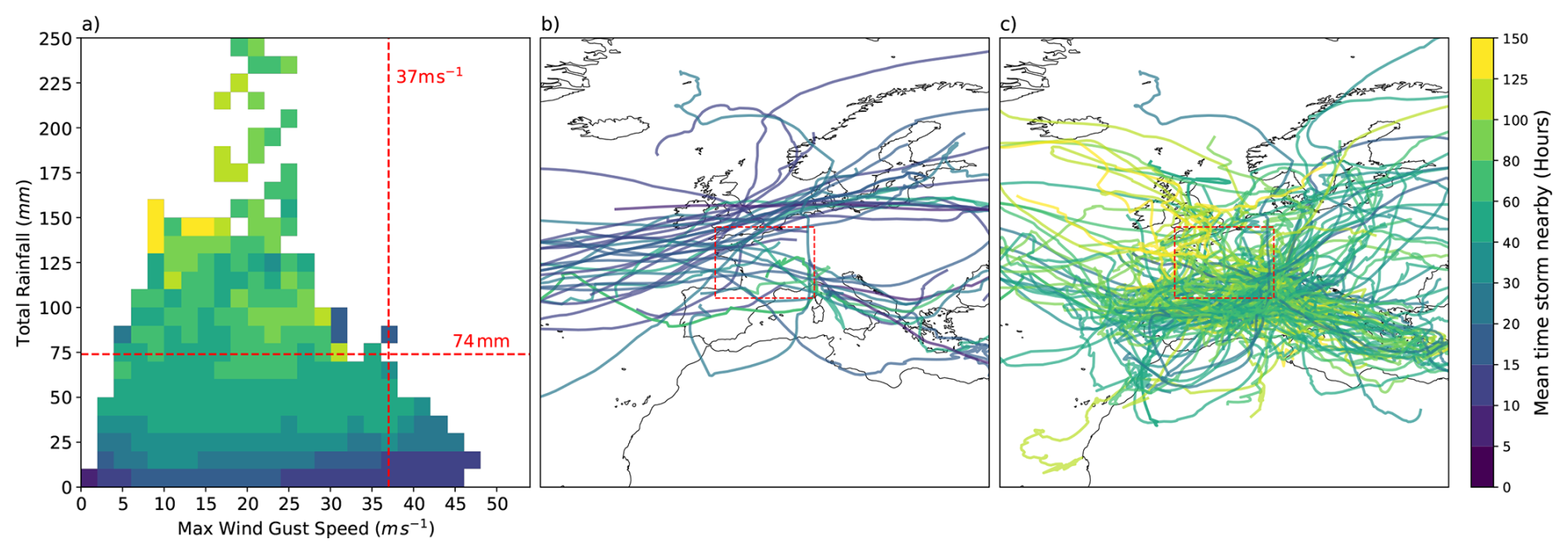
Figure 5 (a) Heatscatter plot of wind gust and precipitation values for France region. Boxes are coloured by mean storm duration. Red dashed lines depict thresholds of 37 m s⁻¹ and 100 mm respectively. (b) Tracks for storms where a grid point had wind speed values above 37 m s⁻¹, (c) Tracks for storms where a grid point had precipitation values above 100 mm. Tracks are coloured by mean storm duration with the same scale as panel (a).

In addition to duration, the previous path of the storm affects moisture availability. Greater poleward propagation speed can increase precipitation rates (Sinclair and Dacre, 2019). Figure 5b and c show tracks of the 42 storms that led to extreme wind speeds > 37 m s⁻¹, and the tracks of the 57 storms that led to total precipitation > 100 mm in France. The extreme wind speed storms tend to have more zonal tracks coming across the Atlantic, whereas the extreme precipitation storms are more meridional with many coming from the south over the Mediterranean. Hence, the duration of storms leading to extremes is also related to where the storms originate – longer duration ones appear to originate more from the south where there is potentially more moisture availability over the warm Mediterranean Sea. Hillier and Dixon (2020) found a similar contrast when considering wind direction on windy and wet locations days. Wind directions at a site on Scotland's east coast were south-westerly on days with extreme wind but north-easterly on days with extreme rain. Hillier et al. (2025) linked this to the location of the jet stream, windier extremes for the UK occurred when the jet was more northerly position. Equivalently high river flows in the UK were associated with a more southerly jet.

This difference may also occur due to the location of wind and precipitation extremes within storm systems. Manning et al. (2024) noticed the track density of precipitation extremes was further south for a box covering the UK and Ireland. This was attributed to wind extremes occurring to the south of the cyclone centre while precipitation extremes occur to the north. When considering a cyclone-centric perspective, Owen (2022) found extremes were similarly located. Relative to a cyclone's centre, wind extremes occur to the south west while precipitation extremes wrap around the east side, with greatest density directly to the east.

By considering annual means of storm duration for each grid point, it is possible to investigate whether duration might be able to account for the interannual dependency between wind and precipitation. Figure 6 shows the correlations between annual mean storm duration $\stackrel{\mathrm{‾}}{D}$ = $S_D/N$ and annual mean intensities, $\stackrel{\mathrm{‾}}{X}$ = $S_X/N$ and $\stackrel{\mathrm{‾}}{Y}$ = $S_Y/N$, at different thresholds. Annual mean duration has a mostly negative correlation with annual mean wind intensity especially over European land regions (Fig. 6a–c), whereas it has a spatially more uniform positive correlation with precipitation intensity (Fig. 6d–f). The magnitudes of these correlations increase over Europe for increasing threshold, which helps to account for why a negative correlation intensifies in the correlation between annual mean wind and precipitation intensities (Fig. 6g–i).

Figure 6 Sample correlations between mean yearly duration and mean yearly wind speed (a–c), mean yearly duration and mean yearly precipitation (d–f), mean yearly wind speed and mean yearly precipitation (g–i). Columns represent different threshold combinations for (u_X,u_Y): no thresholds (0 m s⁻¹, 0 mm) (a, d, g), (10 m s⁻¹, 10 mm) (b, e, h) and high thresholds (20 m s⁻¹, 20 mm) (c, f, i). The statistical significance of sample correlation is shown in Fig. B4.

4 Conclusions

This study has explored collective risk frameworks to model correlation between aggregate severities that occur from multivariate compound events. It has been found that to reproduce the correlation in the wind and precipitation ASIs, it is necessary to include simultaneous correlation between the hazard variables and interannual modulation of the mean hazard variables. Of the three introduced frameworks, only framework C was able to quantitatively capture the correlations across Europe and the North Atlantic at different severity thresholds, including the higher thresholds where negative correlations emerge. Framework C (and the other frameworks) assumed that the hazard variables are independent of the counts and so it does not appear necessary to include severity dependence on frequency as was considered in Hunter et al. (2015) and Cohen (2019). We hypothesise that one of the possible drivers for the interannual modulation is the transit time spent by a storm near to a grid point: total precipitation increases for slower transits, whereas gust speeds tend to increase.

This study has several caveats such as:

• this study has, for simplicity, only considered correlation of ASI that are co-located at the same grid point, whereas the hazards can be displaced from one another but still lead to co-occuring losses for an insured region. Local exposure does not always result in local damage, for example, heavy precipitation at one location may cause flooding much further downstream (Viglione and Rogger, 2015);

• the SIs used here are highly idealised loss functions – a strict cut-off is an unrealistic representation of vulnerability and therefore damage (Kaas et al., 2008);

• absolute thresholds have been used across the whole domain. However, similar results are obtained when using relative thresholds defined by the local quantiles of the hazard variables (not shown);

• the precipitation SI is a proxy for flood but does not contain any information about soil moisture (De Luca et al., 2017) or hydrology that are also required for flood prediction;

• this study has chosen to use the annual aggregation period typical of insurance contracts. Use of other periods, such as individual winters, gives broadly similar results (Fig. B2 in the Appendix);

• the data only spans a relatively short period of 40 years. However, examination of reanalyses going back to 1940 show broadly similar behaviour (not shown due to data quality being poorer in the pre-satellite period);

• ERA5 precipitation is estimated rather than being observed (Hersbach et al., 2020) meaning inaccuracies can exist (Rhodes et al., 2014). Despite reasonable representation of extratropical precipitation (Lavers et al., 2022), ERA5 is not as accurate as station measurements;

• alternative storm tracking algorithms could have been used (see Bourdin et al., 2022) as well as other methods of defining footprints e.g. Vitolo et al. (2009) and Lockwood et al. (2022);

• Pearson's correlation is used as a measure of dependency, this measure can be influenced by outlier events. Furthermore, zero correlation does not always imply independence (Embrechts et al., 2002).

This research could be extended in several ways. It would be of interest to test the effect of relaxing some of the caveats such as the co-located hazard assumption. The framework could also be extended to more than two hazards, which would allow it to be used to investigate compound wind/flood/storm surge losses. Finally, the framework could be applied to output from climate change simulations to understand better how correlation between losses might change in the future. It would also be of interest to better understand what climatic conditions affect storm transit duration in different regions. The speed of the westerly jet and the North Atlantic Oscillation are likely to play key roles, but there may be other factors of interest.

Appendix A: Correlation between aggregated losses

Since frameworks A and B are special cases of framework C, it suffices to derive the correlation for framework C. Using the Law of Total Covariance and the independence of the hazard variables on counts N allows the covariance to be decomposed as follows:

$$\begin{array}{rl}& \text{Cov}(S_X,S_Y)\\ & ={\text{E}}_Z\left[\text{Cov}\right(S_X|Z,S_Y|Z\left)\right]+{\text{Cov}}_Z\left(\text{E}\right[S_X\left|Z\right],\text{E}\left[S_Y\right|Z\left]\right)\\ & ={\text{E}}_Z\left[\text{E}\right[N\left]\text{Cov}\right(X_i|Z,Y_i|Z)+\text{Var}(N\left)\text{E}\right[X_i\left|Z\right]\text{E}\left[Y_j\right|Z\left]\right]\\ & +{\text{Cov}}_Z\left(\text{E}\right[N\left]\text{E}\right[X_i\left|Z\right],\text{E}\left[N\right]\text{E}\left[Y_j\right|Z\left]\right)\\ & =\text{E}\left[N\right]{\text{E}}_Z\left[\text{Cov}\right(X_i|Z,Y_i|Z\left)\right]+\text{Var}\left(N\right){\text{E}}_Z\left[\text{E}\right[X_i\left|Z\right]\text{E}\left[Y_j\right|Z\left]\right]\\ & +\text{E}\left[N{]}^{\mathrm{2}}{\text{Cov}}_Z\right(\text{E}\left[X_i\right|Z],\text{E}[Y_j\left|Z\right]).\end{array}$$

Using the Law of Total Variance, the variance can be decomposed as

$$\begin{array}{rl}& \text{Var}\left(S_X\right)\\ & ={\text{E}}_Z\left[\text{Var}\right(S_X\left|Z\right)]+{\text{Var}}_Z(\text{E}\left[S_X\right|Z\left]\right)\\ & ={\text{E}}_Z\left[\text{E}\right[N\left]\text{Var}\right(X_i\left|Z\right)+\text{Var}\left(N\right)\text{E}\left[X_i\right|Z{]}^{\mathrm{2}}]\\ & +{\text{Var}}_Z\left(\text{E}\right[N\left]\text{E}\right[X_i\left|Z\right])\\ & =\text{E}\left[N\right]{\text{E}}_Z\left[\text{Var}\right(X_i\left|Z\right)]+\text{Var}(N\left){\text{E}}_Z\right[\text{E}\left[X_i\right|Z{]}^{\mathrm{2}}]\\ & +\text{E}\left[N{]}^{\mathrm{2}}{\text{Var}}_Z\right(\text{E}\left[X_i\right|Z\left]\right)\\ & =\text{E}\left[N\right]\left({\text{E}}_Z\right[\text{Var}\left(X_i\right|Z\left)\right]+\mathit{\varphi }{\text{E}}_Z\left[\text{E}\right[X_i\left|Z{]}^{\mathrm{2}}\right]\\ & +\text{E}\left[N\right]{\text{Var}}_Z\left(\text{E}\right[X_i\left|Z\right]\left)\right).\end{array}$$

and a similar expression is obtained for Var(S_Y). Therefore the correlation between S_X and S_Y can be written as

$$\begin{array}{}\text{(A1)}& \begin{array}{rl}\mathit{\rho }& :={\displaystyle \frac{\text{Cov}(S_X,S_Y)}{\sqrt{\text{Var}\left(S_X\right)\text{Var}\left(S_Y\right)}}}\left(\text{Definition of correlation}\right)\\ & ={\displaystyle \frac{\mathit{\theta }+\mathit{\varphi }{J}_{XY}+\mathit{\lambda }{K}_{XY}}{\sqrt{(\mathrm{1}+\mathit{\varphi }{J}_{XX}+\mathit{\lambda }{K}_{XX})(\mathrm{1}+\mathit{\varphi }{J}_{YY}+\mathit{\lambda }{K}_{YY})}}}\end{array}\end{array}$$

where

$$\begin{array}{rl}\mathit{\lambda }& =\text{E}\left[N\right],\mathit{\varphi }={\displaystyle \frac{\text{Var}\left(N\right)}{\text{E}\left[N\right]}}\\ \mathit{\theta }& ={\displaystyle \frac{{\text{E}}_Z\left[\text{Cov}\right(X_i|Z,Y_i|Z\left)\right]}{\sqrt{{\text{E}}_Z\left[\text{Var}\right(X_i\left|Z\right)\left]{\text{E}}_Z\right[\text{Var}\left(Y_i\right|Z\left)\right]}}}\\ J_{XY}& ={\displaystyle \frac{{\text{E}}_Z\left[\text{E}\right[X_i\left|Z\right]\text{E}\left[Y_i\right|Z\left]\right]}{\sqrt{{\text{E}}_Z\left[\text{Var}\right(X_i\left|Z\right)\left]{\text{E}}_Z\right[\text{Var}\left(Y_i\right|Z\left)\right]}}}\\ K_{XY}& ={\displaystyle \frac{{\text{Cov}}_Z\left(\text{E}\right[X_i\left|Z\right],\text{E}\left[Y_j\right|Z\left]\right)}{\sqrt{{\text{E}}_Z\left[\text{Var}\right(X_i\left|Z\right)\left]{\text{E}}_Z\right[\text{Var}\left(Y_i\right|Z\left)\right]}}}.\end{array}$$

The correlation for framework B is obtained by setting all the K terms to zero and J_XY = J_XJ_Y, J_XX = $J_X^{\mathrm{2}}$, J_YY = $J_Y^{\mathrm{2}}$ (because E[X_i|Z] = E[X_i] and E[Y_i|Z] = E[Y_i] are constants and so no longer vary or co-vary). Framework A correlation is obtained from that of framework B by simply setting the event correlation θ to zero.

The parameters in the models are estimated by replacing expectations by sample means:

$$\begin{array}{rl}\mathit{\lambda }=\text{E}\left[N\right]& \to {\displaystyle \frac{\mathrm{1}}{T}}\sum _{t=\mathrm{1}}^T{N}_t=\stackrel{\mathrm{‾}}{N}\\ \text{Var}\left(N\right)& \to \left({\displaystyle \frac{\mathrm{1}}{T}}\sum _{t=\mathrm{1}}^T{N}_t^{\mathrm{2}}\right)-{\left({\displaystyle \frac{\mathrm{1}}{T}}\sum _{t=\mathrm{1}}^T{N}_t\right)}^{\mathrm{2}}\\ {\text{E}}_Z\left[\text{E}\right[X_i\left|Z\right]\text{E}\left[Y_i\right|Z\left]\right]& \to {\displaystyle \frac{\mathrm{1}}{T}}\sum _{t=\mathrm{1}}^T(S_{Xt}/N_t)(S_{Yt}/N_t)\\ {\text{Cov}}_Z\left(\text{E}\right[X_i\left|Z\right],\text{E}\left[Y_j\right|Z\left]\right)& \to \left({\displaystyle \frac{\mathrm{1}}{T}}\sum _{t=\mathrm{1}}^T(S_{Xt}/N_t)(S_{Yt}/N_t)\right)\\ & -\left({\displaystyle \frac{\mathrm{1}}{T}}\sum _{t=\mathrm{1}}^T{S}_{Xt}/N_t\right)\left({\displaystyle \frac{\mathrm{1}}{T}}\sum _{t=\mathrm{1}}^T{S}_{Yt}/N_t\right)\\ {\mathrm{\text{E}}}_Z\left[\text{Cov}\right(X_i|Z,Y_i|Z\left)\right]& \to \left({\displaystyle \frac{\mathrm{1}}{T}}\sum _{t=\mathrm{1}}^T(S_{XYt}/N_t)-(S_{Xt}/N_t)(S_{Yt}/N_t)\right)\\ \text{E}\left(X\right)& \to \left(\sum _{t=\mathrm{1}}^T{S}_{Xt}\right)/\left(\sum _{t=\mathrm{1}}^T{N}_t\right)\\ \text{Var}\left(X\right)& \to \left(\sum _{t=\mathrm{1}}^T{S}_{XXt}\right)/\left(\sum _{t=\mathrm{1}}^T{N}_t\right)\\ & -{\left(\left(\sum _{t=\mathrm{1}}^T{S}_{Xt}\right)/\left(\sum _{t=\mathrm{1}}^T{N}_t\right)\right)}^{\mathrm{2}}.\end{array}$$

where t = $\mathrm{1},\mathrm{2},\mathrm{\dots },T$ is the year and N_t, S_Xt, and S_Yt are the counts and ASI for year t. Similarly S_XYt = ${\sum }_{i=\mathrm{1}}^{N_t}{X}_i{Y}_i$ and S_XXt = ${\sum }_{i=\mathrm{1}}^{N_t}{X}_i^{\mathrm{2}}$. Sample means of the quantities involving sums divided by N were only taken over the years when N_t > 0. Equivalent calculations were computed for E[Y] and Var(Y).

Appendix B: Supplementary figures

Although fixed thresholds are used throughout this study, the frameworks can be applied to SIs that use percentile thresholds. Figure B1 shows the equivalent percentile values for wind gust and fixed precipitation threshold pairs of (10 m s⁻¹, 10 mm) and (20 m s⁻¹, 20 mm). Percentiles are calculated for each gridpoint as the proportion of wind gust and precipitation values below the fixed threshold. The 10 mm threshold is more significant than the 10 m s⁻¹ threshold, as Fig. B1c has higher percentiles than Fig. B1a. Figure B1b shows how a 20 m s⁻¹ wind gust threshold is at least the 95th percentile for most land gridpoints. Figure B1d shows 20 mm is at least the ≈ 98th for most of Northern Europe.

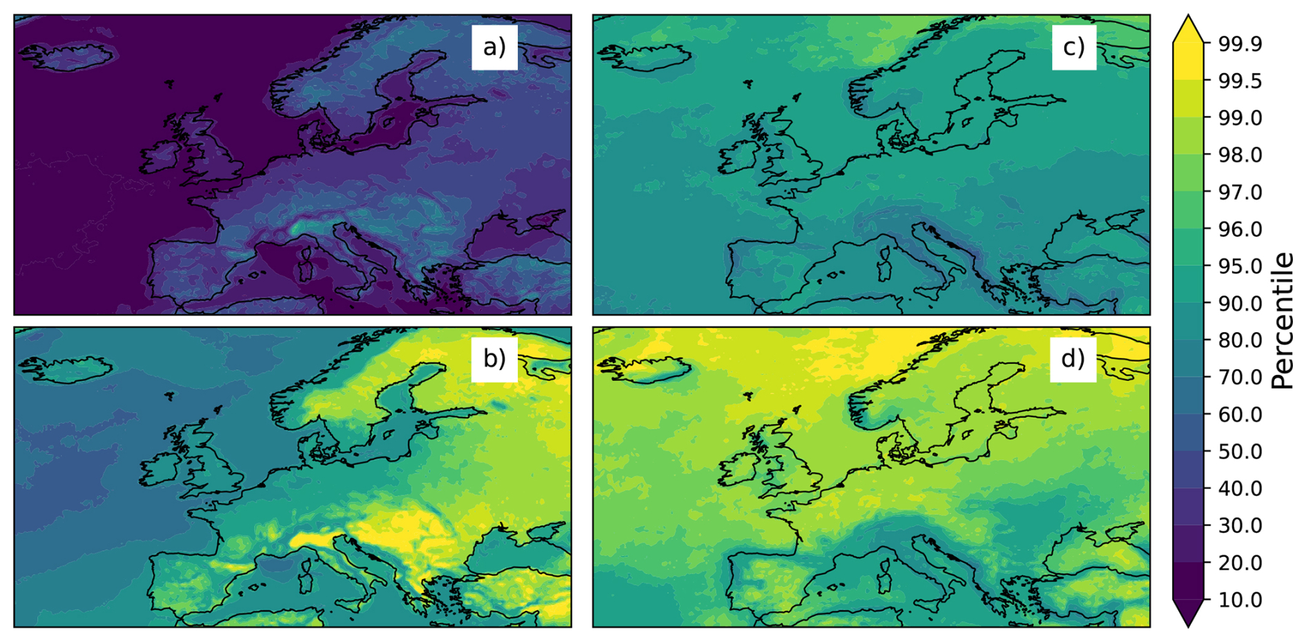
Figure B1 Equivalent percentiles for wind gusts (a, b) and precipitation (c, d) for thresholds u = 10 (a, c) and u = 20 (b, d).

Figure B2 Framework C estimate (a–c) of sample correlation (d–f) for ASIs calculated over the extended winter (1 October–31 March). Sample correlation not significant at the 5 % level is shown by stippling.

Figure B2 shows framework performance ASIs are computed over the extended winter (1 October–31 March). Storms with a genesis time within this period are included. Statistically significant positive correlation occurs at low thresholds (Fig. B2d) while negative values occur at high thresholds (Fig. B2f). Framework C matches this decrease well, although also overestimates negative correlation at the highest threshold (as in Fig. 2l).

Figure B3d–f shows the sample correlation in Fig. 2a–c with stippling added for values not significant at the 5 % level. The near-zero correlation is only significant for most of the region at the lowest threshold. Figure B4 shows Fig. 6 with stippling added for values not significant at the 5 % level. At the highest thresholds sample correlation is robust over most of Europe.

Figure B3 Framework C performance and sample correlation between yearly ASIs. Panels (a)–(c) are the same as Fig. 2j–l. Panels (d)–(f) are the same as Fig. 2a–c but sample correlation not significant at the 5 % level is shown by stippling.

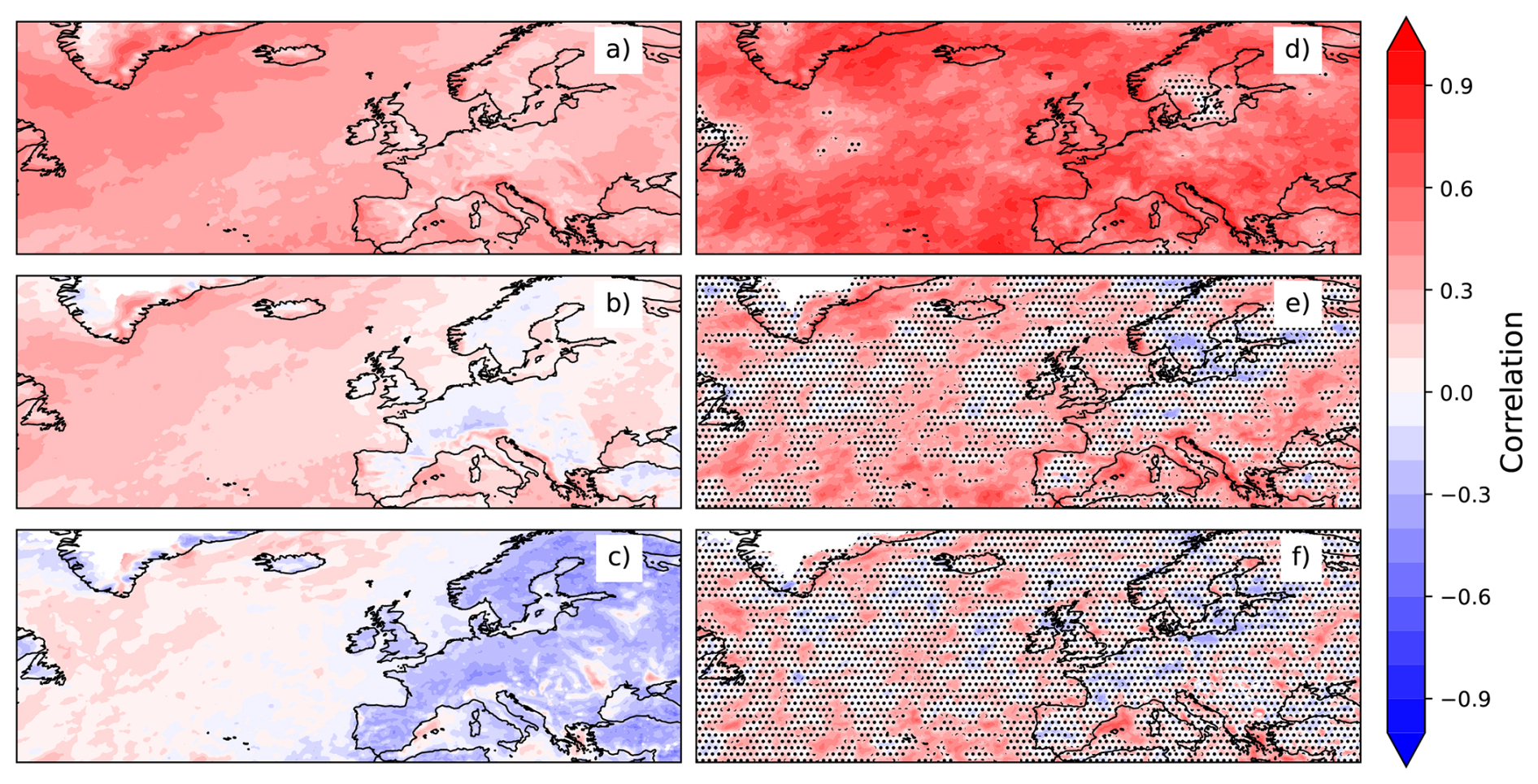
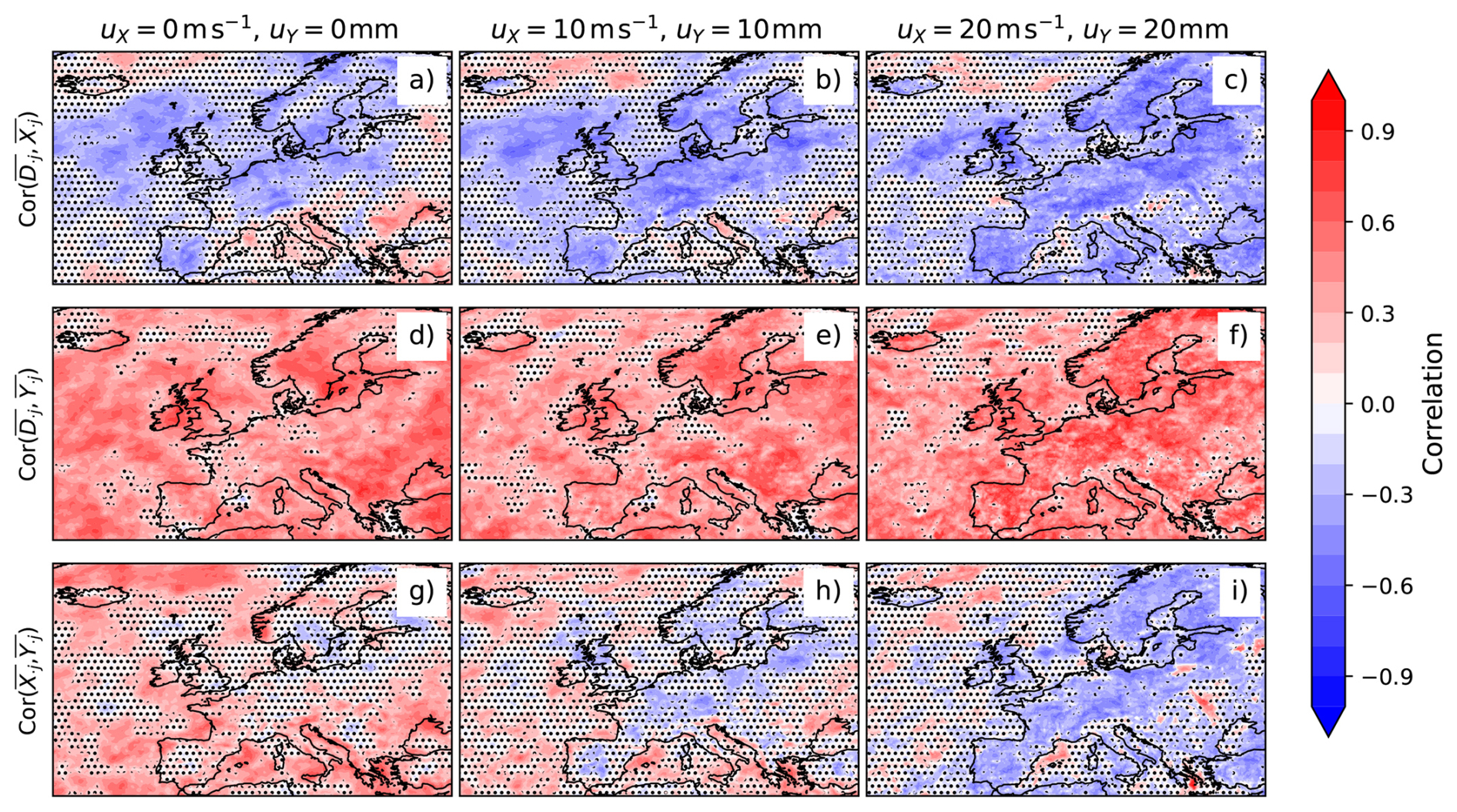
Figure B4 Correlation between mean gust SIs, mean precipitation SIs and mean duration. Same as Fig. 6 but sample correlation not significant at the 5 % level is shown by stippling.