Multiscale modeling for coastal cities: addressing climate change impacts on flood events at urban-scale

This study presents an integrated modeling framework designed to bridge scales from regional to urban, enabling a detailed assessment of the impacts of future climate scenarios on three European coastal cities: Massa (Italy) and Vilanova (Spain) in the Mediterranean, and Oarsoaldea (Spain) in the Atlantic. Conducted as part of the SCORE EU Project (Smart Control of Climate Resilience in European Coastal Cities), the framework employs a novel, non-standard downscaling approach to translate large-scale atmospheric outputs from the EURO-CORDEX regional model ALADIN63 (for Historical, RCP4.5, and RCP8.5 scenarios) into high-resolution simulations of storm surges, wave climate, and river discharge using SHYFEM, WAVEWATCH III, and LISFLOOD models.

The framework achieves coastal resolutions on the order of 100 m, providing time series of water levels and wave runup, which are combined into total water levels. These results, together with extreme value analysis of river discharge and projected relative sea level rise (RSLR), are used as boundary conditions for an urban-scale hydrodynamic model with resolutions as fine as 2–20 m. This multi-scale integration allows for detailed analysis of changes in flooded areas and volumes under RCP4.5 and RCP8.5 scenarios, relative to historical conditions, highlighting the influence of shifting extremes, RSLR, and site-specific features.

Results show that in Massa and Vilanova, increased extreme river discharges are projected, while moderate changes in extreme water levels are overshadowed by RSLR, particularly for Massa. Oarsoaldea, well protected from storm surges, is expected to experience a slight reduction in extreme river discharge. This work demonstrates the capability of an integrated modeling framework to address climate change impacts at the urban scale. Local-scale modeling is essential: accurate flood hazard assessment in coastal cities requires high-resolution simulations to capture the influence of local topography and infrastructure, especially where global DEMs are inadequate. By linking climate projections to urban flood impacts, the framework enables a consistent evaluation of future extremes, sea level rise, and their interaction. A further key message of this study is the need to generate actionable insights to support the development of targeted and site-specific adaptation strategies. Adaptation must be tailored: only by quantifying future extremes and exposure is it possible to design effective, place-based responses.

1 Introduction

Rapid urban growth and climate change are two of the most pressing challenges of our time (Satterthwaite, 2009), especially in coastal regions, where their combination significantly increases the exposure of urban areas to extreme natural events. Coastal cities and settlements, home to more than 2 billion people worldwide, are among the most vulnerable areas to these events (IPCC, 2023; Vitousek et al., 2017; Oppenheimer et al., 2019). Approximately 900 million people live in low-elevation coastal zones (LECZ), areas situated less than 10 m above mean sea level (Reimann et al., 2023), with a projected global population density of around 400–500 people km⁻² by 2060 (Neumann et al., 2015). These regions, marked by increasing anthropogenic activity, hold crucial social and economic importance, with dense population and infrastructure that may further elevate their future vulnerability (Figueiredo et al., 2024; Paranunzio et al., 2022). Global mean sea level is projected to rise between 0.3 and 2 m by 2100 under scenarios of increasing global warming (Vitousek et al., 2017). In addition, the effects of land subsidence are expected to further exacerbate risks in most coastal areas, intensifying future impacts on population and infrastructure (Vousdoukas et al., 2018).

In Europe alone, currently, over 50 million live in LECZ areas (Vousdoukas et al., 2020). With a relative sea level rise (RSLR) of just 0.15 m above 2020 levels, coastal population potentially exposed to a 100-year coastal flood could increase by about 20 % in the medium to long term (IPCC, 2023). By 2100, the total number of people exposed to risk of flooding is projected to reach 1.61 million, and 3.9 million, under the two Representative Concentration Pathways (RCP) scenarios 4.5 and 8.5 (Vousdoukas et al., 2020).

Coastal cities around the world are threatened not only from inundation due to storm surges or sea level rise (Hallegatte et al., 2013; Wahl et al., 2017) but also from river flooding which poses additional risk (Khanal et al., 2019). These areas are therefore impacted by a complex interplay of multiple flood-related systems including river, sea/oceans and coastal land (Laino et al., 2024). Assessing the local effects of such hazards to enhance coastal communities' resilience is one of the greatest challenges of our time, especially in the context of the ongoing climate change. High uncertainty in urban sprawl and flood risks leads to a generalized lack of preparedness to face future flood events (Sun et al., 2022). In this context, high-resolution climate data are essential for defining downscaling strategies that begin with global climate services and are able to evaluate the impacts of multiple hazards at the local scale. Bensi et al. (2020) provides a broad overview of existing literature on hazard interaction, organized by different flooding hazard focus, i.e., studies that address several mechanisms in the fluvial and coastal flood processes alone and studies focusing on joint fluvial and coastal flood processes (e.g., Masina et al., 2015; Bevacqua et al., 2017). Many studies address the degree of dependence among different mechanisms, e.g., precipitation, river flow and storm surge events to assess coastal flood risk, also investigating how it changes over time (Bevacqua et al., 2017; Moftakhari et al., 2017; Orton et al., 2018; Zheng et al., 2013) and with respect to different climate change scenarios (e.g., Parodi et al., 2020; Zhong et al., 2023; Gori and Lin, 2022; Wahl et al., 2015).

Despite the large number of methodologies, tools and models exploring the single or combined effect of climate-related hazards in coastal areas worldwide, studies which exploit different approaches to provide a global multidisciplinary framework to assess flood scenarios in the future at the fine resolution of the urban scale are not widespread (Bensi et al., 2020). Some promising studies pointing in this direction have been developed during the last decade, especially in the US. Based on copulas and bivariate dependence analysis, Moftakhari et al. (2017) quantified the increases in failure probabilities of coastal flood defenses for eight estuarine systems along the coasts of United States caused by RSLR under multiple flood drivers and RCP4.5 and RCP8.5 in 2030 and 2050. To assess climate impacts for the US West Coast, Barnard et al. (2014) used wind fields from different Global Circulation Models (GCMs) under two RCPs scenarios, 4.5 and 8.5, to resolve 3 h peak conditions into the WAVEWATCH III wave models within a deterministic, multidimensional framework in the Coastal Storm Modeling System (CoSMoS). Process-based modeling system proved to be able to dynamically transfer information from global atmospheric scale to the regional and local scale to predict impacts of multiple coastal hazards (i.e., coastal erosion and cliff failures and flooding) for a range of RSLR and storm scenarios at a resolution scale that is relevant for management and adaptation planning (meters scale) (Barnard et al., 2019). In Europe, some few attempts have been made to develop comprehensive models that scale down from the synoptic to the urban scale. Model framework to assess the coastal risks and morphological impacts induced by extreme storm events similar to CoSMoS has been developed in the context of European projects (e.g., Ciavola et al., 2011), but more in support of early warning and emergency response. Van Den Hurk et al. (2015) studied the joint distribution of precipitation and storm surges for 1950 to 2000 using 800 years of simulated data using a RACMO2 Regional Circulation Model (RCM) at 12 km resolution to establish a relation between compound hazards in the Netherlands.

It follows that high resolution RCMs are needed to properly model climate impact at a higher resolution. Estimating the impacts of climate change on coastal cities requires increasing the resolution of city-scale models to unprecedented levels, simulating coastal and terrestrial flood conditions for different return periods and scenarios, and including considerations for the evaluation of financial resilience strategies or ecosystem-based adaptation solutions. Thus, a multidisciplinary framework is needed to foster, through co-participatory and co-creative approach, the public engagement of scientists, policy-makers and citizens, to identify and share socially and technically acceptable solutions. This is part of SCORE project (Smart control of climate resilience in European coastal cities, https://score-eu-project.eu/, last access: 15 January 2025) which aims, through an integrated and multidisciplinary approach, to monitor and validate reliable and robust adaptation measures in low-lying coastal cities to minimize the effects of climate-related hazards and enhance the overall resilience. This is addressed in the context of the Coastal City Living Labs (CCLLs), a novel participatory approach built upon the living lab concept that aims to involve scientists, decision makers, citizens and different stakeholders in the modeling process and in preparing climate risk assessment analysis, thus accelerating the systematic adoption (Paranunzio et al., 2023).

To assess the impacts of multiple climate-related hazards on coastal cities under different climate change scenarios, we present a downscaling procedure which consists of a dynamic multi-branch modeling chain ending with high-resolution (∼ 2 m) flood simulations. Here, we use the term “downscaling” to indicate the transfer of information from the synoptic atmospheric scale to the urban scale of individual buildings and streets, rather than the increase in detail of a specific dataset coming from a numerical model with higher spatial and temporal resolution with respect to the parent one. An integrated approach blending oceanography, hydrology, hydraulics and extreme value analysis (EVA) has been used for the computation of flooded areas for both historical periods and future climate projections for different return periods and under two different RCP scenarios, 4.5 and 8.5 (IPCC, 2014). We used atmospheric data from an EURO-CORDEX RCM (Jacob et al., 2014), and three different models simulating the evolution of water level, wave dynamics, and rainfall-runoff transformation to create the boundary conditions to run hydrodynamic simulations in coastal cities, for both past and future periods. The modeling chain has been applied to the three different CCLLs based on the indications of the SCORE Project: Massa (Italy), Vilanova i la Geltrù and Oarsoaldea (Spain), as different test cases characterized by different phenomenological features.

The high computational demand of the simulation and the need for an extremely fine temporal resolution data are two major challenges in this context. Among the EURO-CORDEX models, only one RCM offers at least three-hourly data for the atmospheric variables required across all models and scenarios. We acknowledge that the use of a multi-RCM (GCM) ensemble is preferable with respect to a single RCM (GCM) to predict more rigorously spatial patterns and to estimate the uncertainty in the projections in response to climate change (Khanal et al., 2019; Gori and Lin, 2022; Bevacqua et al., 2020; Ghanbari et al., 2021). However, the computational cost of the procedure and the high-resolution of the model create challenges for multi-model impact assessment at urban scale. In addition, some studies make successful use of one GCM in dynamical downscaling and hydrological modeling (Vezzoli et al., 2015; Lima et al., 2023).

To our knowledge, this is one of the first works for the European area dealing with projections of climate data at (i) such a high spatio-temporal resolution, (ii) exploiting various computational demanding models up to the urban scale, (iii) seeking to develop a flood hazard modeling chain from multiple sources and (iv) embracing a multidisciplinary modeling framework.

The work is organized as follows. Section 2 provides a brief overview of the project and description of the study sites. Section 3 describes the overall methodology, while Sect. 4 deals specifically with the implementation of the three numerical models. Section 5 describes the extreme value analysis and the urban scale model. Results of the overall methodology are then presented in Sect. 6 and discussed in the next section. Section 8 is dedicated to conclusion on outlook.

2 The SCORE Project and the study sites

The SCORE project focuses on the resilience of coastal cities to the effects of climate change. Coastal cities, as climate change hotspots, are affected by numerous consequences resulting from changes in the marine, atmospheric, and terrestrial (hydrogeological) components of the Earth system. However, among the many risks related to climate change in coastal cities (which could include increasing marine and atmospheric heatwaves, fire risks, subsidence due to the over-exploitation of water resources in tourist areas, etc.), SCORE has focused on flood risk. This includes flooding from rivers, marine inundations, or a combination of both. Marine floods, as is well known, can result not only from extreme storm surges but from combinations of storm waves and high tidal levels (both astronomical and meteorological induced by wind and pressure), following a signal that is modulated in the long term by RSLR.

The selection of cities involved in the project was made during the project development phase. The choice was not driven by prioritizing cities with the highest exposure to these effects (e.g., the city of Venice), but rather those where there is an active and engaged community of citizens, stakeholders, and research centers collaborating on co-designing solutions to improve resilience to the effects of climate change. This process begins with ecosystem-based adaptation solutions (EbAs; Munang et al., 2013; Temmerman et al., 2013; Tiwari et al., 2022), which encourage practices that increase citizen participation and awareness, such as sharing meteorological observations following Citizen Science standards (Conrad and Hilchey, 2010). The modeling components developed for these cities also contribute to the creation of urban-scale Digital Twins, which are part of a specific activity within the project. These digital tools, alongside advanced data representation, enable a better understanding of flood effects and allow the modeling of adaptation scenarios using a What-If methodology (Paranunzio et al., 2023).

Within the project, local initiatives are built following the Living Lab paradigm (Bulkeley et al., 2018), forming Coastal Cities Living Labs, where local communities participate according to the quadruple helix model (Carayannis and Campbell, 2009). The decision of whether cities would act as frontrunners or followers for certain project activities (as organized through the project work packages) was made based on the specific themes of interest within the CCLLs.

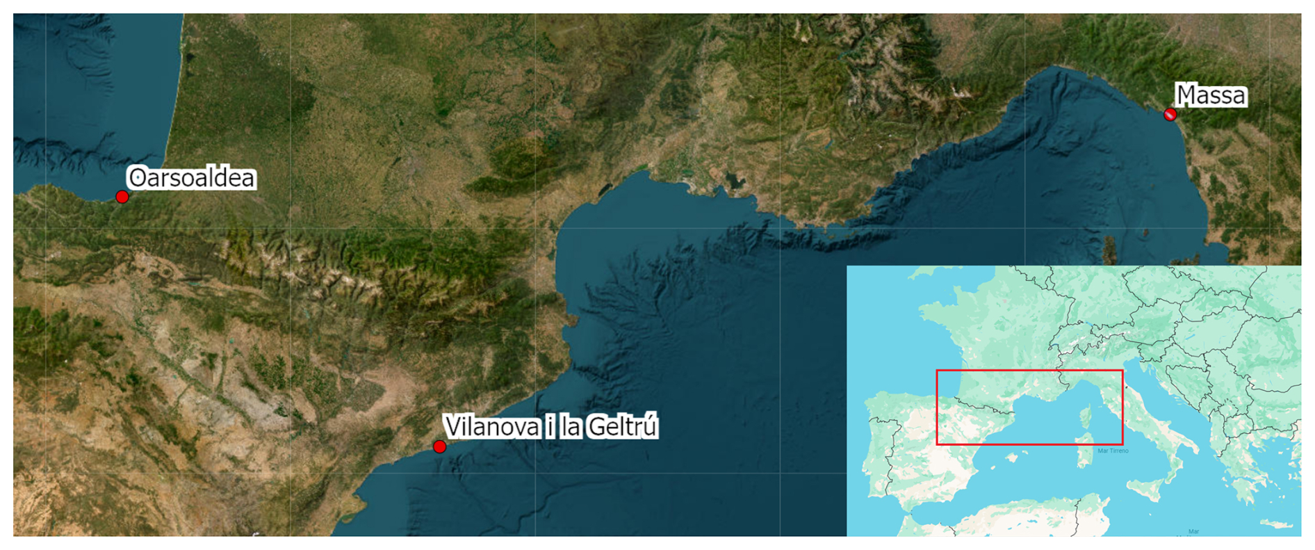
Figure 1 View of the geographical area where the analyzed cities are located. Maps data: © Google Earth 2024; images: © CNES/Airbus, Maxar Technologies, Airbus.

Therefore, the selection of the study cases presented in this article: Massa, Vilanova i la Geltrù (from now on we will refer to the city simply as Vilanova), Oarsoaldea (Fig. 1) was based on the presence of three frontrunners that followed a common analysis methodology, which is described in the next section. This methodology starts from the availability of data provided by climate services and, through downscaling techniques and urban and coastal hydraulic modeling, defines the design conditions expected for coastal cities. Defining case studies based on project guidance does not diminish the scientific value of this work or the approach used; rather, it demonstrates how the problem of coastal resilience is universal and not restricted to specific areas. Ultimately, this requires a careful analysis that can be more effectively carried out with a local and site-specific approach rather than relying solely on regional models, even when they have high-resolution.

3 Overall methodology

The modeling chain implemented transfers information from the atmospheric synoptic scale (1000–100 km) up to the urban scale (2 m), and is aimed at obtaining time series of wave height H_s, water level η, and river discharge Q close to the coastal cities of interest, for both past periods and future climate projections. An extreme value analysis is then performed on the calculated time series to estimate the peak values associated with specific return periods. These values are eventually employed to build synthetic events to simulate their effects in terms of flooded areas for the analyzed coastal cities. A sketch of the overall procedure is reported in Fig. 2.

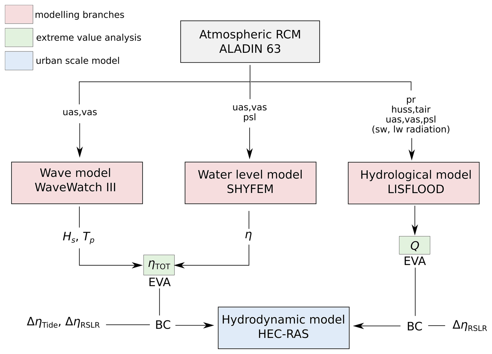
Figure 2 Sketch reporting the overall methodology to downscale data and run hydrodynamic simulations at the urban scale. Light red boxes correspond to the models employed to downscale atmospheric variables, light green boxes contain variables subject to extreme value analysis and the light blue box corresponds to the urban scale flood modeling part. H_s is the significant wave height, T_p is the peak wave period, Q is the river discharge, η is the water level, Δη_Tide and Δη_RSLR are the increases in water level due to tide and relative sea level rise, respectively.

The modeling chain implemented employs atmospheric data from the ALADIN63 RCM (Coppola et al., 2020; Vautard et al., 2020), provided by the EURO-CORDEX experiment (Jacob et al., 2014), and use it as input for the following models: WaveWatch III (WW3DG, 2019a) simulates the dynamic of wave height taking as input the surface zonal and meridional wind velocities (uas, vas); SHYFEM (Umgiesser et al., 2004) simulates the evolution of water levels forced by surface winds (uas, vas) and mean sea level pressure (psl); LISFLOOD (Van Der Knijff et al., 2008) simulates the rainfall-runoff transformation and takes in input several atmospheric variables such as rainfall rate (pr), air temperature (tair), specific humidity (huss), sea level pressure (psl) shortwave and longwave radiation (rsds, rlds, rsus, rlus). A more detailed and thorough description of the downscaling procedure for each variable is reported in Sect. 4.1, 4.2 and 4.3.

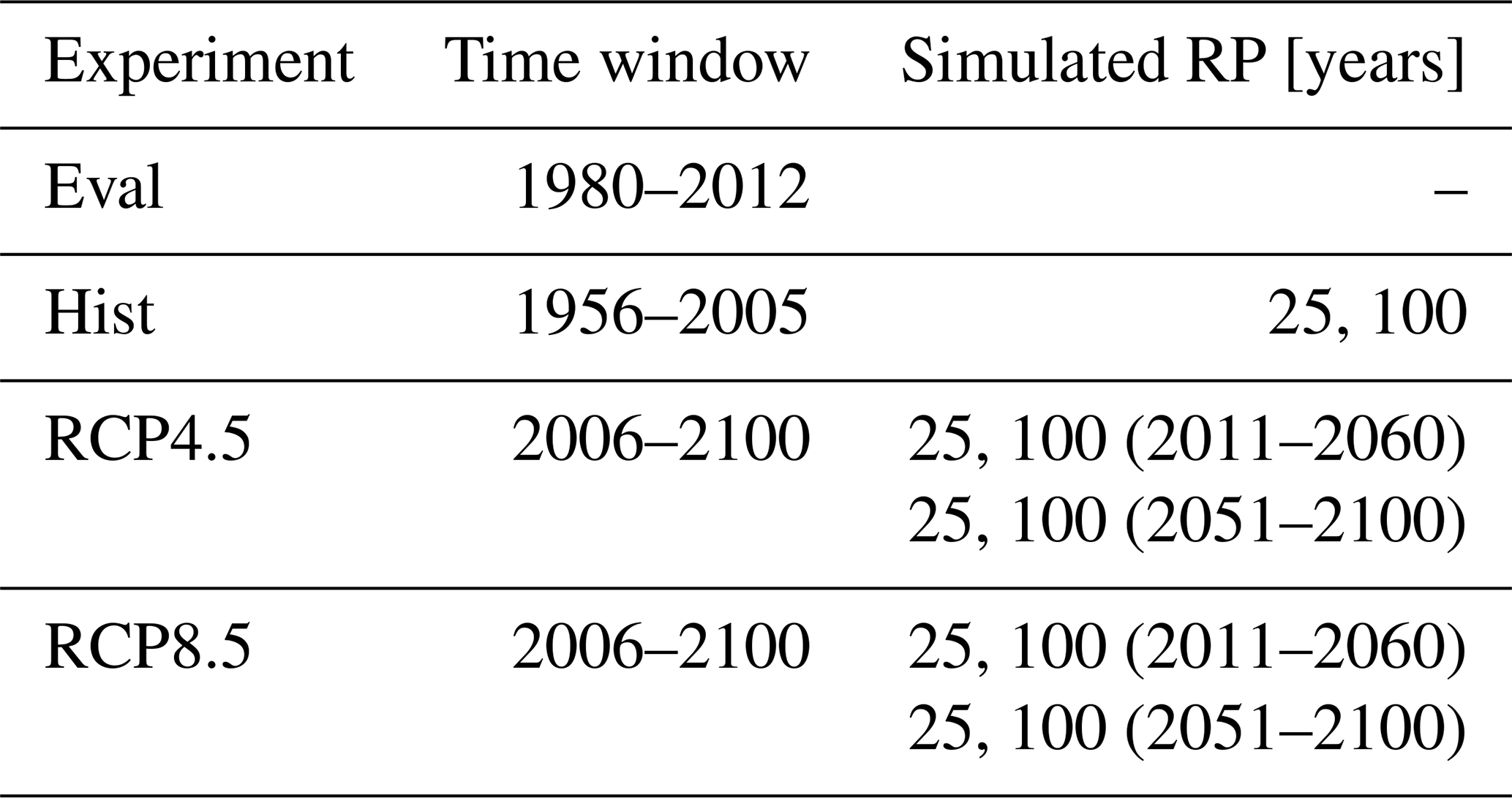
For each of the models, the Evaluation, Historical, RCP4.5 and RCP8.5 experiments are simulated. The Evaluation (Eval) experiment is employed to test the ability of the model to reproduce observable extreme events. In such a case the ALADIN63 RCM is forced by the ERA-Interim reanalysis (Dee et al., 2011). The Historical (Hist) experiment is used as a baseline for the two climate change scenarios expressed by the Representative Concentration Pathways defined by the fifth Assessment Report (AR5) of Intergovernmental Panel on Climate Change (IPCC, 2014). RCP4.5 and RCP8.5 data are used to analyze the effect of anthropogenic climate change in the future flooding pattern at urban scale. For this set of simulations, the ALADIN63 RCM was forced by the CNRM-CM5 GCM (Voldoire et al., 2012). The choice of such a RCM is due to the fact that this was the only one that provided at least three-hourly data for the atmospheric forcing variables for all the experiments, among the EURO-CORDEX models. Other RCMs provided those variables at different output frequencies or solely for specific temporal windows (e.g. RCP4.5 for the period 2050–2070 and RCP8.5 for the period 2030–2050). The consequences and limitations of such a choice are discussed in Sect. 7.

A summary of the simulated experiments with associated time windows is reported in Table 1.

Table 1 Summary of the simulated experiments with associated time windows. Return periods (RP) refer to the values calculated through the extreme value analysis and used to create synthetic events simulated with the urban scale hydrodynamic model.

The hydrodynamic simulations of storm surges and river flood at urban scale have been performed using the HEC-RAS 6.4 model (Brunner and US Army Corps of Engineers, 2021), similarly to Gori and Lin (2022). The storm surge is modeled following a simplified approach consisting of the combination of time series of wave runup R_2 % and water level. First, the wave runup R_2 % is determined using wave height and period and the slope of the beach, following Atkinson et al. (2017), then, it is added to the water level η, to obtain the total water level η_TOT. The extreme value analysis is carried out on this last variable and on the river discharge Q, separately, for all the simulated experiments (Table 1). Hazard maps reporting the water depth envelope associated with a specific return period event are produced for the flood due to the storm surge and for the riverine flood. Furthermore, to simulate the RSLR and the effect of the tide, an increased value for the mean water level is applied to each hydrodynamic simulation based on the associated experiment. A more detailed description of the urban scale hydrodynamic modeling activity is reported in Sect. 5.

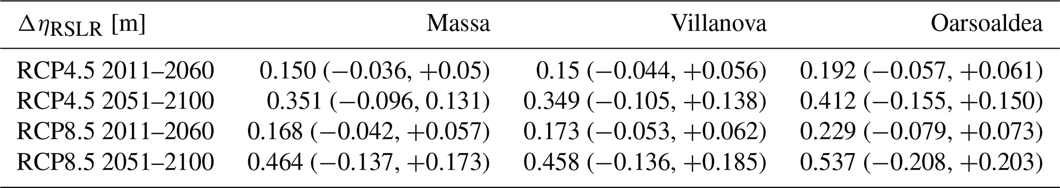
The projections of RSLR for RCP4.5 and RCP8.5 used in this paper can be found in two free-access datasets (Vousdoukas et al., 2016a, for RCP4.5 data, Vousdoukas et al., 2016b, for RCP8.5 data), downloadable from the European Commission Joint Research Centre (JRC) website. These datasets provide the Total Water Level (TWL), from which the RSLR can be extracted by subtracting the episodic extremes (wave runup and storm surge level) which are also provided, along with the tidal contribution. More information can be found in the related article (Vousdoukas et al., 2017). The dataset covers the European coastlines with a temporal resolution of 10 years. Europe is divided into 10 regions, within which all values are averaged. All values are given with respect to the 1985–2005 reference period.

4 Modeling branches

In this section, we describe the implementation of the three numerical models: WaveWatch III, SHYFEM and LISFLOOD, employed to perform the main part of the downscaling procedure. Each of the models has a particular setup on the basis of the analyzed coastal city. Furthermore, a calibration/validation procedure has been carried out for each of them to have an estimate of their skill to reproduce observed events. The detailed description of the different procedures is reported in the Supplement.

4.1 Wave climate model

The numerical model used to simulate wind waves was WaveWatch III (WAVE-height, WATer depth and Current Hindcasting), v. 6.07 (WW3DG, 2019a), a community third-generation wave model developed at the US National Centers for Environmental Prediction (NOAA/NCEP) that includes the latest scientific advancements in the field of wind-wave modeling and dynamics (https://github.com/NOAA-EMC/WW3/releases/download/6.07/wwatch3.v6.07.tar.gz, last access: February 2022).

WAVEWATCH III solves the random phase spectral action density balance equation for wavenumber-direction spectra, and includes options for shallow-water applications. Propagation of a wave spectrum can be solved using regular (rectilinear or curvilinear) and unstructured (triangular) grids. Source terms for physical processes include parameterizations for wave growth due to the actions of wind, nonlinear resonant wave-wave interactions, scattering due to wave-bottom interactions, triad interactions, dissipation due to whitecapping, bottom friction, surf-breaking, and interactions with mud and ice. Source terms are integrated in time using a dynamically adjusted time stepping algorithm.

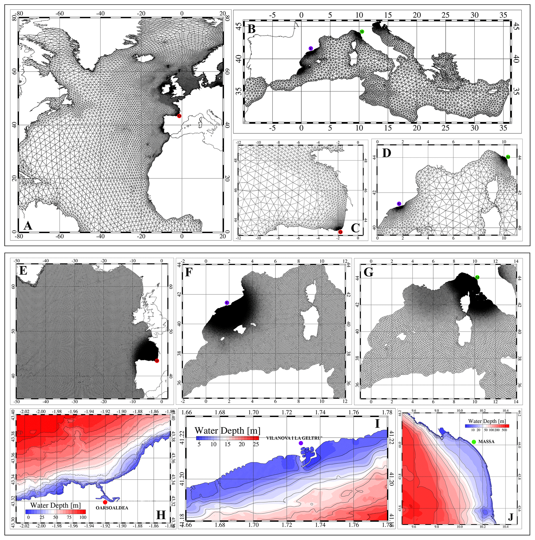
Figure 3 Finite element meshes used by the WWIII wave model (upper panels labeled with A, B, C and D) and the SHYFEM hydrodynamic model (lower panels labeled with E, F, G, H, I and J). Panels (A) and (B) show portions of the WWIII domains, which include most of the Atlantic Ocean and the entire Mediterranean Sea. High-resolution areas for Oarsoaldea (red point), Vilanova (blue point), and Massa (green point) are displayed in panels (C) and (D). Panels (E), (F), and (G) illustrate portions of the three SHYFEM domains, covering most of the North Atlantic Ocean and the entire Mediterranean Sea, highlighting the high-resolution areas. The bottom panels (H, I, J) depict the bathymetric details of the three study sites.

In this application, according to the project needs, two different implementations of the model were performed, with two different computational domains. The first one included the entire Mediterranean basin and a further area west of the Strait of Gibraltar, to improve accuracy in the Alboran Sea (Fig. 3b). The second one was extended to the Atlantic Ocean (Fig. 3a) to simulate the wave climate in front of the ocean-facing European cities. As for boundary conditions, domains were assumed to be closed at the farthest ocean boundaries. Both domains have been discretized by unstructured meshes with a variable resolution up to 500 m in the coastal areas surrounding the cities of interest (Fig. 3c and d). The resolution decreases in the rest of the domain and the minimum resolution in deep offshore areas reaches about 70 km for the Mediterranean grid, and about 300 km for the Atlantic one. GEBCO, EMODnet, and nautical chart bathymetries were used in different parts of the domains.

The output of the wave model was recorded hourly at all grid points for the integrated quantities, in particular significant wave height (H_s), mean wavelength (L_m), mean wave period (T_m), peak wave period (T_p), mean wave direction (Dir_m) and peak wave direction (Dir_p). The atmospheric dataset provided by ERA Interim+EuroCordex (ALADIN63 RCM) for the evaluation data and CMIP5+EuroCordex (Taylor et al., 2011) for the other data, which includes wind (uas, vas) at a frequency of 3 h, was used as forcing.

4.2 Water level model

Future projections of storm surge events for the three study sites have been conducted using advanced numerical modeling techniques. Specifically, SHYFEM (System of Hydrodynamic Finite Element Modules, Umgiesser et al., 2004), an ocean model based on the finite element method, has been implemented for each coastal site to simulate the temporal and spatial variability of water levels influenced by atmospheric forcing, wind and atmospheric pressure.

SHYFEM is an open-source community model (freely downloadable at https://github.com/SHYFEM-model/shyfem.git, last access: March 2022), that resolves the 3D primitive equations system, integrated over z-layers, in their formulations with water levels and transports. It uses a semi-implicit algorithm for the discretization in time and finite element for the spatial integration. The model has been widely used to investigate the main hydrodynamics in coastal areas (e.g. Western Mediterranean Sea in Bonamano et al., 2024; Cucco et al., 2023, 2022; Umgiesser et al., 2014, 2022; Quattrocchi et al., 2021; Maicu et al., 2018; Federico et al., 2017) and for real time prediction of storm surge events in several coastal sites in the Mediterranean sea, e.g. the Venice Lagoon (Umgiesser et al., 2022; Bajo et al., 2007, 2019). We refer to (Umgiesser et al., 2004) for a detailed overview of the model equation system, numerical treatment and parameters setup.

In this application, SHYFEM has been implemented in 2D mode accounting for barotropic pressure gradients, wind drag and bottom friction, which are the primary forces driving the storm surge events (Bloemendaal et al., 2018; Wicks and Atkinson, 2017). The model was applied to simulate the atmospheric contribution to water level η, thus neglecting the non-linear interaction with tides. This approach is commonly used in ocean prediction systems, in fact, the non-linear interactions between tides and surge are generally small enough to allow for the linear addition of tidal and surge components thus reducing the complexity of numerical experiments (Yang et al., 2023; Zijl et al., 2013; Bajo et al., 2007).

The water levels including tides can be derived by adding the astronomical tide to the computed η. The impact on accuracy depends on tidal amplitudes, which are minimal in the Western Mediterranean Sea due to very low tides (0.2–0.3 m) and slightly more significant for the Atlantic site where tidal amplitudes exceed 1.5 m (around 3 m, as estimated by Fernández-Montblanc et al. (2018) for the whole European coastal seas). The same assumption was applied to other factors such as general circulation and climate-induced RSLR, which contribute to a lesser extent to water level fluctuations in case of extreme events.

Three different finite element meshes have been implemented to reproduce, with varying spatial resolution, the geomorphological features of the three coastal sites (Fig. 3h, i, l). Each domain extends to the entire basin facing each study site (the Western Mediterranean Sea for Villanova and Massa, and most of the North Atlantic for Oarsoaldea) to cover the full area influenced by the main wind fetches and to eliminate the need for ad hoc open boundary conditions.

The atmospheric dataset provided by the ALADIN63 RCM, which includes wind and atmospheric pressure data (uas, vas and psl) at a 3 h frequency, was used as forcing.

4.3 River discharge model

River floods occur when the stream or channel geometry is not sufficient to contain the incoming volume of water. In order to model river floods, it is necessary to define the inflow discharge hydrograph as a boundary condition, i.e. the evolution in time of flow rate in the upstream cross section. The shape of the hydrograph, the time and value of its peak, and in general the streamflow generated in the channel network as a response to precipitation events, are the consequences of the hydrological processes in the upstream basin. Such processes include several complex mechanisms occurring at land surface (infiltration, evapotranspiration, runoff generation, hillslope routing, snowmelt, groundwater recharge) that depend on many factors like basin topography, soil hydraulic properties, vegetation cover and structure of the river network. Moreover, the downstream boundary condition defined by the water level at the outlet affects the evolution of the hydrograph while traveling along the river (see Sect. 5.2).

In this work, we have used LISFLOOD (https://ec-jrc.github.io/lisflood/, last access: January 2022), a spatially distributed hydrological model developed by the Joint Research Centre (JRC) of the European Commission since 1997 (Van Der Knijff et al., 2008). LISFLOOD has been applied to a wide range of applications and is currently used in the EFAS (European Flood Awareness System) and GLOFAS (Global Flood Awareness System) (Alfieri et al., 2019). In LISFLOOD, the soil is schematised with three layers and all the main hydrological processes are modeled: surface runoff, exchange of soil moisture between layers and drainage to the groundwater, sub-surface and groundwater flow and flow through river channels.

For the calculation of potential reference evapotranspiration, potential evaporation from bare soil and open water, LISFLOOD can be coupled to the LISVAP preprocessing routine (JRC, 2013), especially developed for this purpose (https://ec-jrc.github.io/lisflood-lisvap/, last access: January 2022).

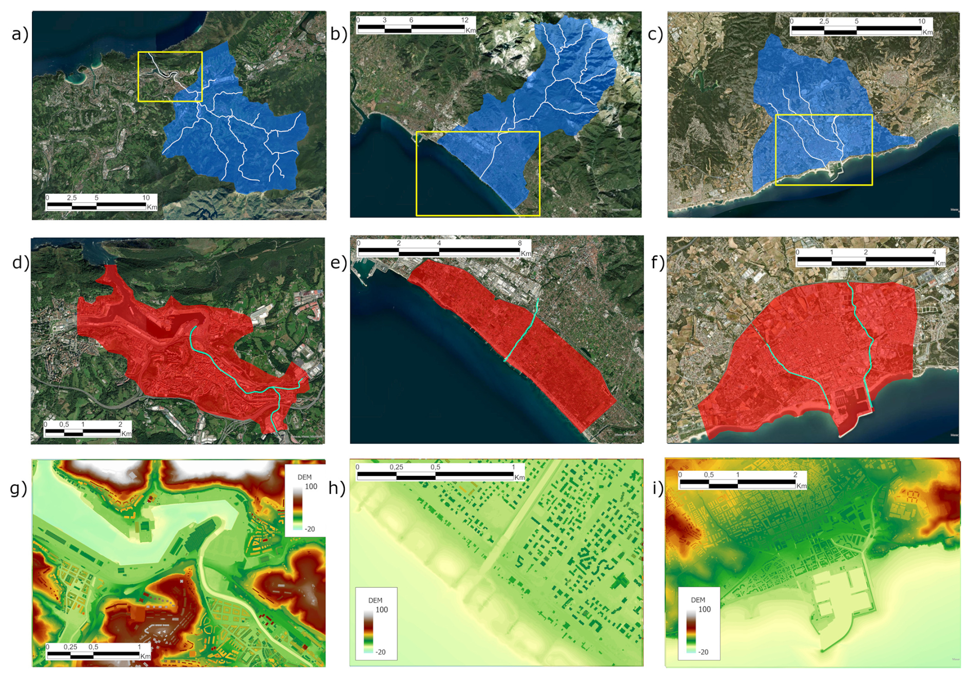
Figure 4 Top row: View of the domains (blue shading) for the rainfall-runoff hydrological model: (a) basin of Oiartzun river, with outlet in Oarsoaldea, (b) basin of Frigido river, with outlet in Massa (b), basins of Torrent de San Juan and Torrent de la Piera, with outlet in Vilanova (c). Middle row: View of the domains of the 2D hydrodynamic modeling (red shading): (d) Oarsoaldea, (e) Massa, (f) Vilanova. Bottom row: Enlargement of the area close to the river mouth, showing the resolution of the employed DEM to create the 2D computational domain: (g) Oarsoaldea, (h) Massa, (i) Vilanova. Base map: Maps data: © Google Earth 2024; images: © CNES/Airbus, Maxar Technologies, Airbus.

In this work LISFLOOD model was applied to the main rivers that cross the selected coastal cities: Frigido river for Massa (catchment size ∼ 70 km²), Torrent de la Piera and Torrent de San Juan for Villanova (total size of the two catchments ∼ 40 km²), and Oiartzun river for Oarsoaldea (catchment size ∼ 85 km²). Such watersheds were represented as gridded domains with 100 × 100 m cell size (Fig. 4a, b, c).

For Frigido river, geomorphological and land cover characteristics were obtained from data available from Tuscany Region (hydrologically conditioned DEM at 10 × 10 m resolution, land cover at 1 : 10 000 scale), while for the other basins data were obtained from EU-DEM v 1.1 25 × 25 m resolution, Copernicus Land Monitoring Service (https://land.copernicus.eu, last access: March 2022) and ISRIC Soil Grids 250 × 250 m (https://www.isric.org, last access: March 2022).

The meteorological forcing fields extracted from EURO-CORDEX necessary to run the LISFLOOD-LISVAP models, as reported in Sect. 3, are precipitation (1 h), sea level pressure (3 h), wind speed (3 h), minimum and maximum air temperature (daily), humidity (daily), shortwave and longwave radiation (daily).

Output of LISFLOOD are the times series of hourly river discharge in selected points, for each climatological scenario. Extreme value analysis can then be applied on these long-term time series to obtain design flood peaks for the selected return periods and the resulting hydrographs to be used as BC for the hydraulic simulations (whose domains are shown in Fig. 4d, e, f), as described in Sect. 5.

5 Modeling floods at urban-scale

In this section, we describe the extreme value analysis to obtain the boundary conditions for the flood simulations at urban scale using the hydrodynamic model implemented at each analyzed city.

5.1 Extreme value analysis

The extreme value analysis has been performed for the variables river discharge Q and total water level η_TOT. Two return period values were determined, 25 and 100 years for each experiment (Historical, RCP4.5, RCP8.5). Furthermore, for the climate projections, two different time windows were analyzed, 2011–2060 and 2051–2100 (Table 1).

In this study, the Generalized Extreme Value (GEV) distribution was employed to model the occurrence of annual maxima values of river discharge Q and total water level η_TOT, separately. Since our principal objective is the comparison among different experiments, such a distribution allowed us to be consistent and to use the same number of events (50) for all the experiments.

The total water level η_TOT for the Massa and Vilanova cases is equal to the sum of η and the runup value, which is calculated with the Atkinson et al. (2017) equation: $R_{\mathrm{2}\mathit{\%}}=\mathrm{0.92}\tan \mathit{\beta }\sqrt{H_{\mathrm{S}}{L}_{\mathrm{P}}}+\mathrm{0.16}{H}_{\mathrm{S}}$, where tan β is the slope of the beach and L_P is the deep water wavelength at the peak period. Before the calculation of R_2 %, the wave height is projected along the orthogonal direction to the coastline, to account for wave direction. For Oarsoaldea the effect of runup is not included in the computations since we do not simulate waves within the port.

The Generalized Extreme Value (GEV) distribution can be written as follows (cumulative distribution function):

$$\begin{array}{}\text{(1)}& F\left(x\right)=e^{-{\left(\mathrm{1}+\mathit{\xi }\frac{x-\mathit{\mu }}{\mathit{\sigma }}\right)}^{-\frac{\mathrm{1}}{\mathit{\xi }}}}\end{array}$$

defined for values of x for which $\mathit{\xi }\cdot x>\mathit{\xi }\cdot \mathit{\mu }-\mathit{\sigma }$. In this equation, μ is the location parameter, ξ is the shape parameter, and σ is the scale parameter. The shape parameter ξ governs the distribution type: ξ=0, Type I, Gumbel distribution; ξ>0, Type II, Fréchet distribution; ξ<0, Type III, Weibull distribution (Coles, 2001).

The parameters μ, σ, ξ are estimated from data using the maximum likelihood method. Then, the return levels x_RP for a given return period can be calculated as follows:

$$\begin{array}{}\text{(2)}& x_{\mathrm{RP}}=\mathit{\mu }+{\displaystyle \frac{\mathit{\sigma }}{\mathit{\xi }}}\left(\left(-\ln {\left(\mathrm{1}-{\displaystyle \frac{\mathrm{1}}{\mathrm{RP}}}\right)}^{-\mathit{\xi }}\right)-\mathrm{1}\right).\end{array}$$

To ensure robust estimates of the uncertainties associated with the return levels, the confidence intervals (CI) at the 95 % significance level were calculated using parametric bootstrapping with 500 iterations (Gilleland, 2020). The statistical analysis has been performed using the R package extRemes: Extreme Value Analysis (Gilleland and Katz, 2016).

5.2 Hydrodynamic model

The effect of extreme storm surge and river flood on the analyzed coastal cities was determined using the HEC-RAS 6.4 hydrodynamic model (Brunner and US Army Corps of Engineers, 2021). The software couples the simulation of the flow within a river, solving the one-dimensional Saint-Venant equation, to the two-dimensional flow on the floodable areas, solving the shallow water equations. Once the water level within the river bed exceeds the elevation of the levees, water flows on the two-dimensional computational mesh (the opposite flow is also possible).

The computational domains associated with the three cities are reported in Fig. 4d, e, f. Each mesh is created by overlapping the HEC-RAS computational grid to the digital elevation model (DEM) of the analyzed area. The system calculates specific elevation-volume relationships for each computational cell, representing the details of the underlying layer. This allows us to save computational time by setting a lower resolution for the HEC-RAS mesh with respect to the DEM. For the three cities of Massa, Vilanova and Oarsoaldea, the DEM is obtained from the LIDAR dataset, at a resolution of 2 m (Fig. 4g, h, i), merging it to information from nautical charts, except for the city of Massa, where two single beam surveys were available for the years 2012 and 2017. The HEC-RAS mesh elements have a reference size from 10 to 20 m, except for specific areas (e.g. close to the coastline, complex urban patterns, etc..) where they are reduced to 5 m. The river geometry is composed by the river cross sections and additional information of hydraulic structures. For the Massa and Oarsoaldea cases the geometry comes from a topographic survey, whereas for Vilanova it was extracted from the LIDAR dataset.

Table 2 Combination of upstream and downstream boundary conditions for the river and coastal flood simulations.

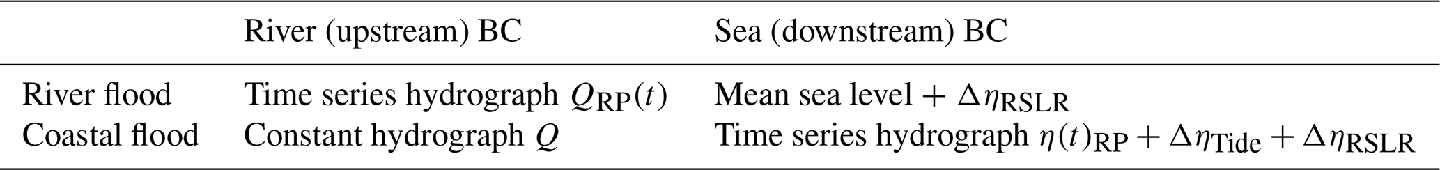
Boundary conditions (BCs) are differently set based on the simulation carried out, as reported in Table 2. For the river flood simulations the upstream BC is a time series Q_RP(t), with peak discharge value Q_RP equal to the return period value. The shape of the hydrograph Q_RP(t) is determined as follows: (i) the 24 h preceding and following the annual maxima are extracted for each year; (ii) these 49 h time series are superimposed to have maxima in phase and then averaged; (iii) the averaged time series is normalized to obtain q(t), having maximum equal to 1; (iv) the Q_RP(t) boundary is obtained multiplying q(t) by Q_RP. Such a procedure is applied to every run to get the appropriate BC. The figures showing the superimposition of the annual maxima events for river discharge and water level for the three cities of Massa, Villanova and Oarsoladea, are reported in the Supplement. The downstream BC at the sea is the mean sea level plus the RSLR, based on the reference scenario Δη_RSLR as reported in Table 2.

Table 3 Values of RSLR referred to the RCP4.5 and RCP8.5 scenarios, averaged over the reference period, for the analyzed cities. All values are given with respect to the 1985–2005 reference period. Data extracted from Vousdoukas et al. (2016a) (RCP4.5 data) and Vousdoukas et al. (2016b) (RCP8.5 data).

For the coastal flood simulations, considering the inaccuracies inherent in long-term predictions on a century time scale (Dessai et al., 2009), a statistical approach was preferable to take into account tides and other factors contributing to the water level of the downstream BC. Specifically, for each site, delta water levels representing the maximum spring tidal amplitudes Δη_Tide (0.2 m for Massa and for Villanova) and the predicted sea level rise on a decadal time scale Δη_RSLR (Table 3) were linearly added to the η_RP(t) time series to estimate the worst-case scenario for coastal flooding. η_RP(t) is calculated following the same procedure employed for the river discharge, with peak value equal to η_TOT,RP. This approach does not take into account long-term trends potentially present in the tidal constituents as observed by Santamaria-Aguilar et al. (2017). The upstream BC is a constant value for the river discharge such as the model can run without instabilities and no flood occurs.

In Oarsoaldea, we used a slightly different approach for the coastal flood simulations since the tidal excursion is larger than the extreme return period values: the downstream BC is a semidiurnal tide (up to 2.3 m) added to the Δη_RSLR and to the increase due to the return period value Δη_RP.

For the city of Massa a single river called Frigido is simulated and the urban area is divided into two portions adjacent to the sides of the river (Fig. 4d). In Villanova, two river streams are modeled, the easternmost is the main one, called Torrent de la Piera, whereas the other one (Torrent de Sant Joan) is forced underground for about 500 m, just before the rivermouth (Fig. 4e). The two-dimensional domain is split in three subdomains, one between the two rivers and two on their sides. Oiartzun is the main river modeled for Oarsoaldea, while Lintzirin is its tributary forced underground for most of its length (Fig. 4g). In this case the peak discharge of the minor river is scaled in proportion to the basin area (47.4 and 8.7 km², respectively). The two-dimensional domain is divided into two parts including the Pasaia bay area.

6 Results

6.1 Extremes for wave climate, water level and river discharge

A first comparison is performed between the annual maxima of the Historical and Evaluation runs. For the former, the years from 1973 to 2005 are considered, whereas for the latter those from 1980 to 2012, for an overall amount of 33 years each. This allows us to have an estimate of the degree of over/under-estimation we can have on the projections with respect to the actual scenario.

In Fig. 5, the quantile-quantile plots for the three analyzed cities for both river discharge and total water level are reported. Historical and Evaluation annual maxima total water levels in Massa are in agreement (Fig. 5a), whereas Historical river discharge is subject to underestimation only for the highest values (Fig. 5b). Total water levels in Villanova are generally larger for the Historical run with respect to Evaluation (Fig. 5c), whereas river discharge extreme values are correctly estimated except for a single data (Fig. 5d). Oarsoaldea water levels are slightly overestimated by the Historical up to 0.4 m. Also river discharge values are generally overestimated up to 100 m³ s⁻¹, then, the largest values tend to be underestimated (Fig. 5f). As a result of the calibration and validation procedure, we also noticed the tendency of the evaluation run to underestimate observed extremes measured by wave buoys (see Supplement, Fig. S12).

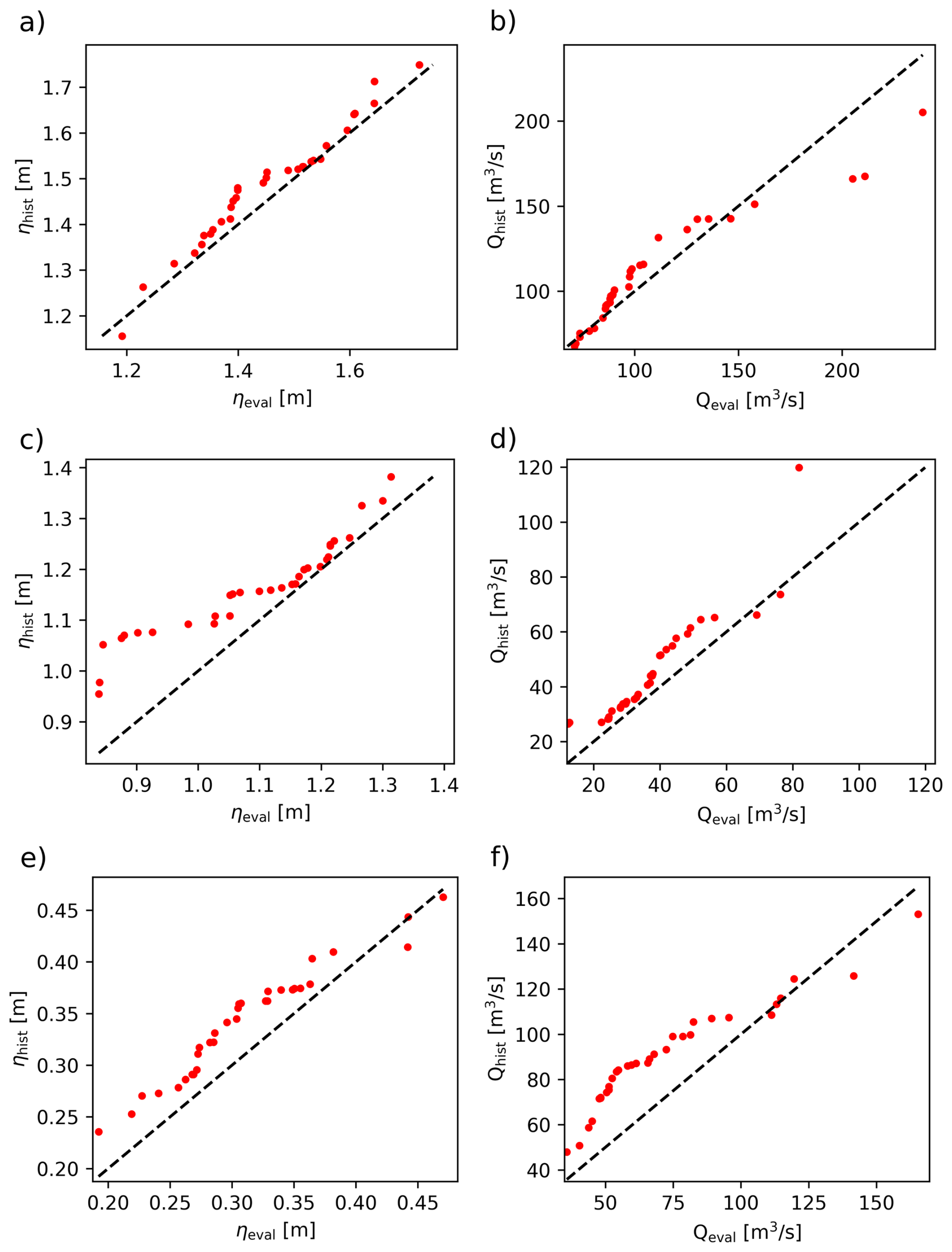
Figure 5 Quantile-quantile plots between annual maxima from evaluation and historical runs, for the city of Massa (a, b), Villanova (c, d), and Oarsoaldea (e, f) for the total water level ηTOT (first column), and the peak discharge Q (second column). For the city of Oarsoaldea η is reported since no runup contribution is considered. Red dots represent the annual maxima, black dashed line is the 1 : 1 line.

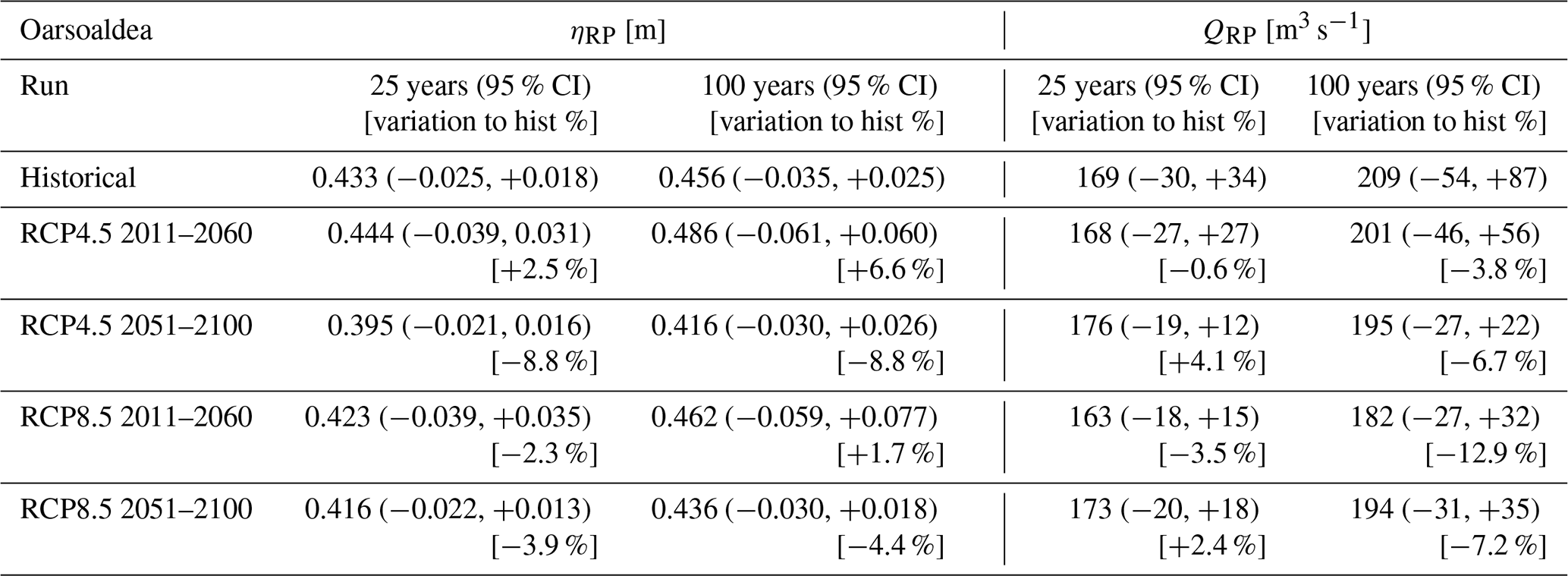
Tables 4, 5 and 6, show the results of the extreme value analysis of η_TOT,RP and Q_RP for the city of Massa, Villanova and Oarsoaldea, respectively, together with the confidence intervals at 95 % significance level (round brackets) and the percentage increase/decrease (square brackets) with respect to the Historical values.

Table 4 Return period values associated with 25 and 100 years for the different runs for the city of Massa for both the total water level η_TOT,RP and the peak discharge Q_RP. Numbers in % (in square brackets) represent the variation relative to the historical value.

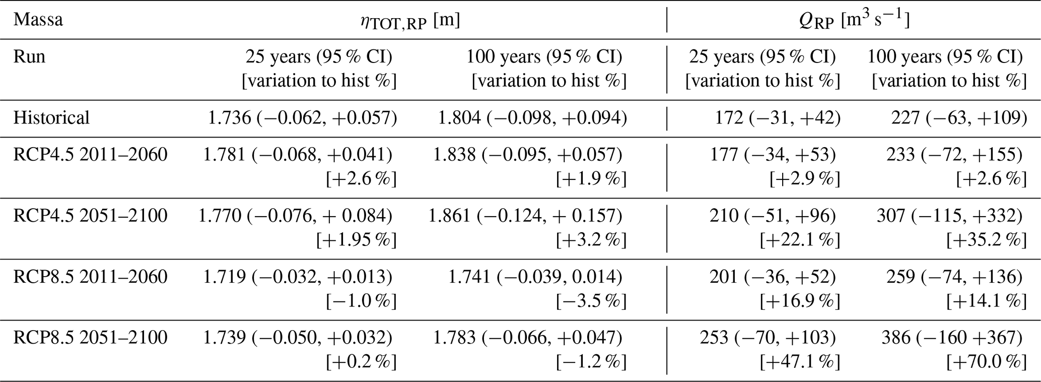
Table 5 Return period values associated with 25 and 100 years for the different runs for the city of Villanova for both the total water level η_TOT,RP and the peak discharge Q_RP. Numbers in % (in square brackets) represent the variation relative to the historical value.

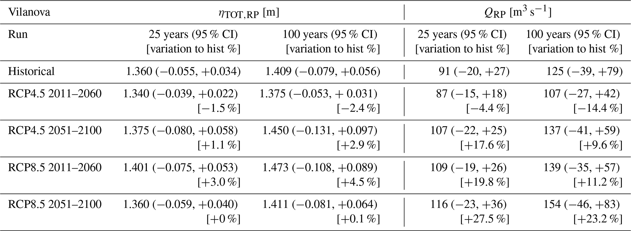
Table 6 Return period values associated with 25 and 100 years for the different runs for the city of Oarsoaldea for both the water level η_RP and the peak discharge Q_RP. Numbers in % (in square brackets) represent the variation relative to the historical value.

For η_TOT in Massa, the RCP4.5 scenario shows slightly larger values with respect to the historical run, whereas the RCP8.5 has similar or slightly lower values. Conversely, extreme Q values tend to grow for both time windows and further forward in the future for both RCP4.5 and RCP8.5. Nevertheless, the estimated 100 years peak discharge shows large uncertainty values, especially for the 2051–2100 case for both RCP4.5 and RCP8.5 runs (Table 4).

Extreme η_TOT values for the city of Villanova show an increase for the RCP4.5 2051–2100 and for the RCP8.5 2011–2060 scenarios (both 25 and 100 years RPs), whereas a decrease is found for the RCP4.5 2011–2060. Analogously, Q extreme values are lower than the historical for the RCP4.5 2011–2060 scenario (both 25 and 100 years RPs), but an increase is observed for all the other cases (Table 5).

Concerning extreme water levels in Oarsoaldea, an increase for the RCP4.5 2011–2060 (both 25 and 100 years RPs) is observed, while all the other cases show decrease or substantial invariance. The extreme river discharge is not subject to significant variations for the 25 years RP, whereas a general slight decrease is observed for the 100 years RP for all scenarios.

6.2 Flooded areas

The envelope of the water depth, that is the spatial distribution of the maximum water depth reached at each computational cell during the hydrodynamic simulation, are reported in Figs. 6 and 7 for coastal and riverine floods with a 100 years RP, respectively.

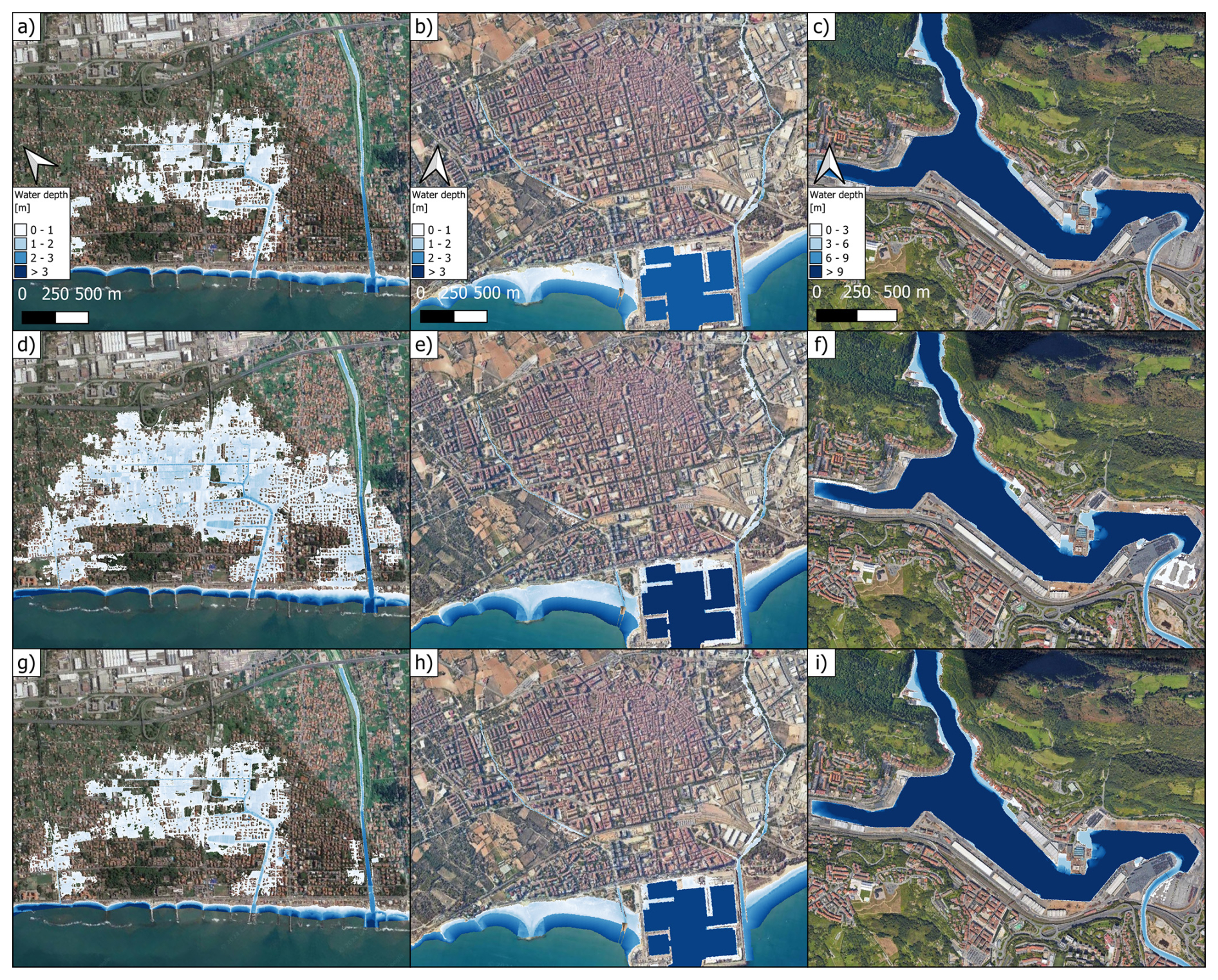
Figure 6 Hazard maps associated to the 100 years return period coastal flood event for the city of Massa: historical (a), RCP4.5 2051–2100 (d), RCP8.5 2011–2060 (g); for the city of Vilanova: Historical (b), RCP4.5 2051–2100 (e), RCP8.5 2011–2060 (h); for the city of Oarsoaldea: historical (c), RCP4.5 2051–2100 (f), RCP8.5 2011–2060 (i). Maps data: © Google Earth 2024; images: © CNES/Airbus, Maxar Technologies, Airbus.

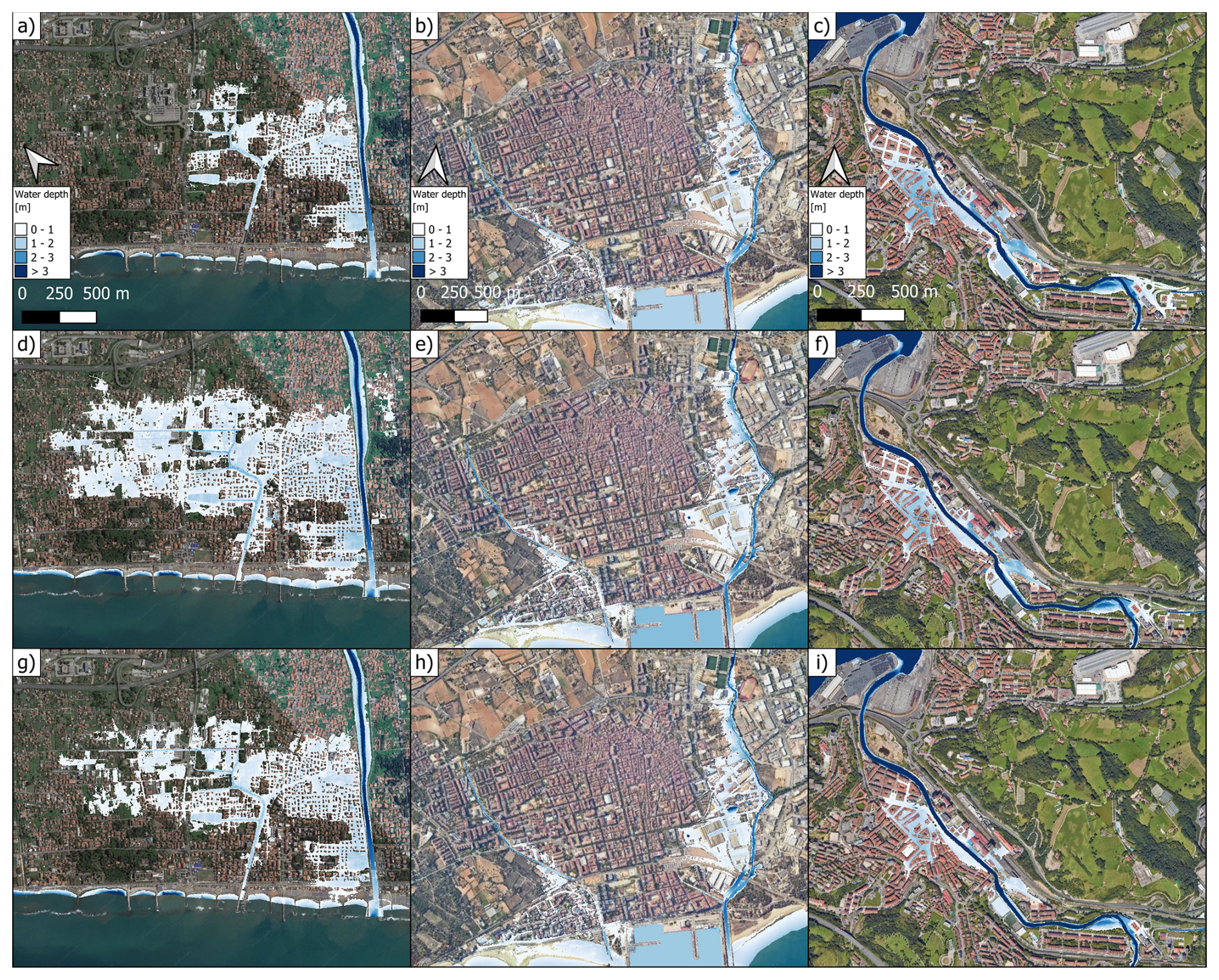
Figure 7 Hazard maps associated to the 100 years return period riverine flood event for the city of Massa: Historical (a), RCP4.5 2051–2100 (d), RCP8.5 2011–2060 (g); for the city of Vilanova: historical (b), RCP4.5 2051–2100 (e), RCP8.5 2011–2060 (h); for the city of Oarsoaldea: historical (c), RCP4.5 2051–2100 (f), RCP8.5 2011–2060 (i). Maps data: © Google Earth 2024; images: © CNES/Airbus, Maxar Technologies, Airbus.

More specifically, results are reported for the RCP4.5 2051–2100 and RCP8.5 2011–2060 for the three analyzed cities. The remaining figures of flooded areas, that is: the 100 years RP coastal floods (Fig. S1) and 100 years RP riverine floods (Fig. S2) cases, and all the 25 years RP cases (Fig. S3 for coastal flood and Fig. S4 for riverine flood), are reported in the Supplement.

Table 7 Percentage change of the flooded volume with respect to the historical run for the three cities of Massa, Vilanova and Oarsoaldea, for the RCP4.5 and RCP8.5 (2011–2060, 2051–2100) scenarios for both the 25 and 100 years return periods.

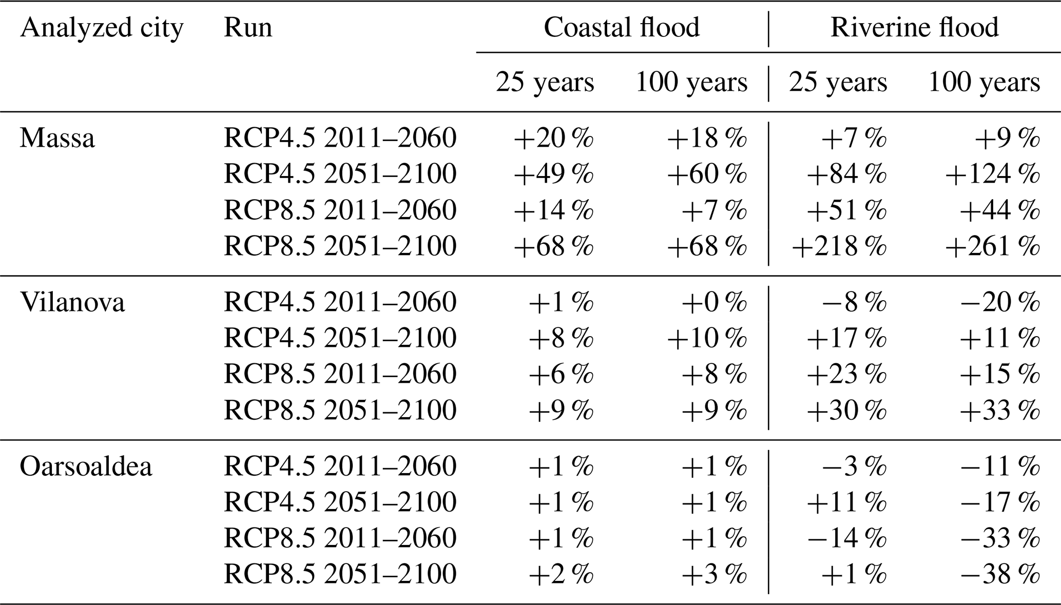
For the city of Massa, the simulations of the future scenarios show an increase in flooded areas, especially for the RCP4.5 2051–2100 (Fig. 6a, d, g). Such a case shows a rise of 60 % in flooded volume with respect to the Historical case, whereas the increase is 7 % for the RCP8.5 2011–2060 100 years RP (Table 7). In general, coastal flood volume increase in Massa is larger for the furthest time window in the future.

Storm surges in Villanova mainly impact the beach area and the surroundings of the port (Fig. 6b, e, h), and the rise in flooded volume compared to the Historical case is at most 20 % (RCP4.5 2051–2100 25 years RP, Table 7).

For Oarsoaldea, the hydrodynamic simulations of coastal flooding do not show substantial variations between the Historical case and the projections (Fig. 6c, f, i). This is confirmed by the flooded volume variation which is at most 3 % for the RCP8.5 2051–2100 100 years RP (Table 7).

The results of the 100 years RP riverine floods hydrodynamic simulations are reported in Fig. 7. For the city of Massa a substantial increase in the flooded area for the RCP4.5 2051–2100 (Fig. 7d) and RCP8.5 2011–2060 (Fig. 7g) with respect to Historical case (Fig. 7a), is observed. This is consistent with the rise in flooded volume reported in Table 7, where an increase larger than 200 % is seen for both the RPs associated with the RCP8.5 2051–2100 case.

The visual comparison of Fig. 7b, e, h does not allow to clearly detect an increase/decrease in flooded area with respect to the Historical case for the city of Vilanova. However, the computation of flooded volume variation shows an increase up to 33 % for all cases except for RCP4.5 2011–2060 for both RPs (Table 7).

Oarsoaldea exhibits a different behavior since the Historical events cause larger floods with respect to most part of the projections. Even for this city the visual comparison of water depths does not allow us to identify increase/decrease in flooded areas (Fig. 7c, f, i), but the results reported in Table 6 show that rise in flooded volume around 11 % is observed only for the 25 years RPs for the RCP4.5 for the 2051–2100 time window. All other cases show a decrease in flooded volume, up to −38 % for RCP8.5 2011–2060 100 years RP.

7 Discussion

Assessing the impacts of future climate scenarios on extreme flood events in coastal cities requires a huge effort due to the need to integrate processes across multiple scales, from synoptic scale (i.e. storms spanning ∼ 100–1000 km) to local scale. At the urban scale, specific geomorphic features such as landscape elevation and structural elements can significantly influence flood extent. To address this complexity, we implemented a multiscale modeling chain tailored for three of the CCLLs under the SCORE Project, but that can be easily generalized to other coastal cities. We employed unstructured grids modelling approaches to simulate wave climate (WWIII) and water levels (SHYFEM). These were integrated with the distributed hydrological model LISFLOOD, and finally coupled within high-resolution urban hydrodynamic simulations, to capture the interaction between extreme events and urban-specific characteristics, achieving the spatial granularity needed to capture critical urban-scale flood dynamics. However, this level of detail comes with a huge computational effort: each of the three models ran simulations equivalent to nearly 300 years, repeated for all analyzed cities.

This consideration was the most significant factor influencing our choice of using a single RCM (and GCM) rather than a multi-model ensemble approach. In addition, data availability from EURO-CORDEX for all required variables at a sufficient output frequency and covering the Evaluation, Historical, RCP4.5 and RCP8.5 runs was ensured only by the ALADIN63 model driven by the ERA-Interim reanalysis and the CNRM-CM5 GCM. We have given priority to have a continuous dataset at the cost of giving up an uncertainty estimate based on a multi-model ensemble. We tried to partially compensate for the lack of such an uncertainty estimation, by calculating confidence intervals through the bootstrap method in the statistical analysis, although this is a different source of uncertainty.

The comparison between the annual maxima from the Evaluation and Historical runs (Fig. 5), together with the information reported in Tables 4, 5 and 6, enables us to assess the reliability of the coastal and riverine hazard maps (Figs. 6 and 7).

If we only look at the return period values of total water level for the city of Massa, we do not observe significant variations in terms of event magnitude compared to the Historical period. Indeed, the increase/decrease ranges from −3.5 % to +3.2 with a predominance of positive values (Table 3). Considering the 95 % CIs, the variability generally lies between ±2.5 % and ±5 % of the calculated extreme value for the 2011–2060 and 2051–2100 time windows, respectively. Although an increase in wave height is projected for the Ligurian-Tyrrhenian Sea (De Leo et al., 2024), several factors may contribute to the observed invariance in total water levels for Massa. The shallow bathymetry in front of Massa (Fig. 3) can act as a sort of filter for the highest offshore waves, leading to a sort of upper limit for the wave height close to the shoreline which, in turn, affects the total water level through the runup equation. Additionally, the very high resolution of the modeling near the coast captures local-scale effects that are often missed by lower-resolution models. Furthermore, the sensitivity of runup to wave height for Massa's beach slope, calculated using wavelengths ranging between 70 and 95 m (those associated with the highest waves) is modest, approximately 0.2–0.25 m. This means that a 1 m increase in wave height produces 0.2–0.25 m increase in runup. As a consequence, any increase/decrease in wave climate is partially damped. Actually, the main driver behind the significant differences in flooded volume is the Relative Sea Level Rise (RSLR) (Table 3), which allows storm surges to penetrate farther inland, resulting in larger flooded volumes (Table 7). This finding is consistent with the conclusions of the IPCC Sixth Assessment Report (IPCC, 2023), which states that regional sea level change will be the primary factor contributing to a substantial increase in the frequency of extreme still water levels over the next century, even assuming other contributors to extreme sea levels to remain constant. Therefore, all uncertainties in sea level rise projections can significantly affect the flood extension and volume associated with extreme events. In addition, the projected sea level rise by the end of the century could be significantly higher if the less likely, but still plausible, ice-sheet-related dynamics were to occur (IPCC, 2023, 2014).

Riverine floods for the RCPs projections in Massa show a substantial increase, even more evident for the 2051–2100 time window. However, this is accompanied by an equal increase in uncertainty. Indeed, the width of the 95 % CI is almost 1.5 times the 100 years RP for both the RCP4.5 and RCP8.5 2051–2100. Despite this, the overall increase in extreme Q_RP for all the analyzed scenarios and time windows confirms an increase in future peak river discharges. However, such extremes could be slightly underestimated as observable from the QQ-plot of Evaluation and Historical annual maxima (Fig. 5b). Indeed, we make the hypothesis that the Evaluation run, being a reanalysis, is close to reality given that it benefits from a data assimilation procedure, thus incorporating the information from observations. Notwithstanding, their impact on the ground is further augmented by the increase in relative sea level, whereby the higher downstream boundary condition hinders the flow toward the sea, resulting in a substantial increase in the flooded volume (Table 7).

The extension of the flooded area for Vilanova appears not to be affected by storm surges principally due to the characteristics of the beach zone which is separated from the urban area by a steep positive gradient in the land elevation which makes the latter higher. A substantial equivalence between the Historical and the RCP4.5 and RCP8.5 extreme values is observed and the Δη_RSLR ranges between 0.15 and 0.458 m (Table 3). Even though the increase in flooded volume is always positive (Table 7), the flooded area is not enlarged (Fig. 6b, e, h) and the only area which is interested in an enlargement of the flooded surface is the one adjacent to the port.

The riverine floods associated with projections are generally characterized by an increase in flooded volume with respect to the Historical (from +11 % to +33 %), but for the RCP4.5 2011–2060 25 and 100 years RPs (−8 % and −20 %), as reported in Table 7. Concerning the Q_RP values, the higher the extreme value, the larger the CI width. However, a substantial increase in river discharge is observable, in agreement with the flooded volume. The comparison of annual maxima from Evaluation and Historical (Fig. 5d) suggests no underestimation/overestimation, even if the largest value could lead one to think of an overestimation. The additional increase in flooded volume (Table 7) compared to the maxima in river discharge (Table 5) is primarily attributed to the RSLR, similar to the findings for Massa.

For the city of Oarsoaldea the port area has been designed to face tidal excursions around 2 m. The extreme values associated with both 25 and 100 years RP range between 0.395 and 0.486 m. Table 5 reports increases (RCP4.5 2011–2060) and decreases (RCP4.5 2051–2100 and RCP8.5 2051–2100) of the extreme water level for the projections compared to the Historical, consistent with the findings of Vousdoukas et al. (2017). The modest rise in flooded volume (+1 % to +3 %, Table 7) is mainly attributable to the RSLR.

For river discharge, a generalized decrease in peak Q_RP values is observed, with the width of the 95 % CI of the same order of magnitude of the variation with respect to the Historical period, and an expected slight underestimation of the projected extremes (Fig. 5f).

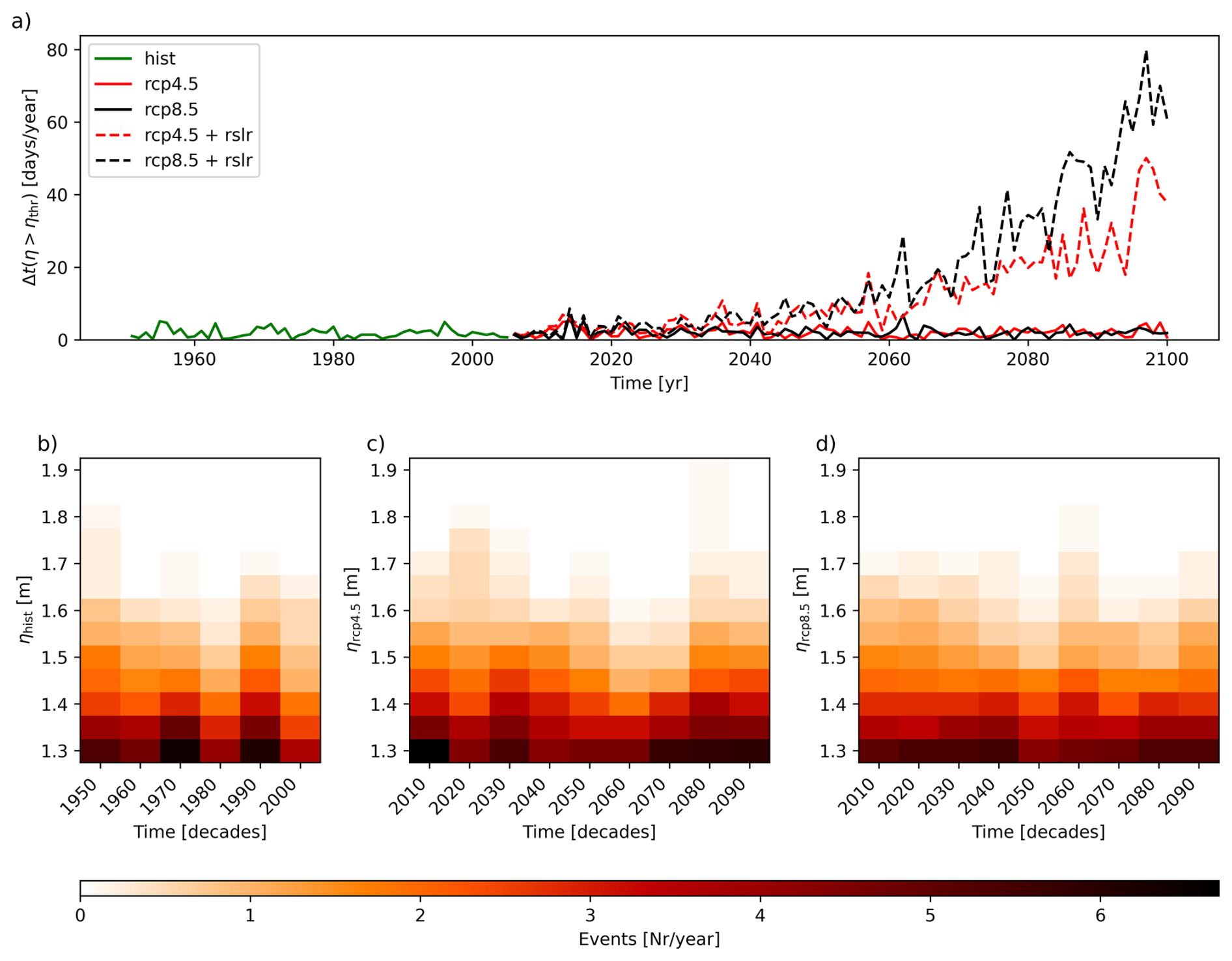
Figure 8 (a) Cumulative duration of total water level above the 99.5 %-ile in days per year for HIST (green line), RCP4.5 (red line), RCP8.5 (black line), RCP4.5 and RCP8.5 plus the effect of RSLR (red dashed line and black dashed line, respectively), for the city of Massa. Number of events per year with peak values larger than specific values, grouped by decades for: HIST (b), RCP4.5 (c) and RCP8.5 (d).

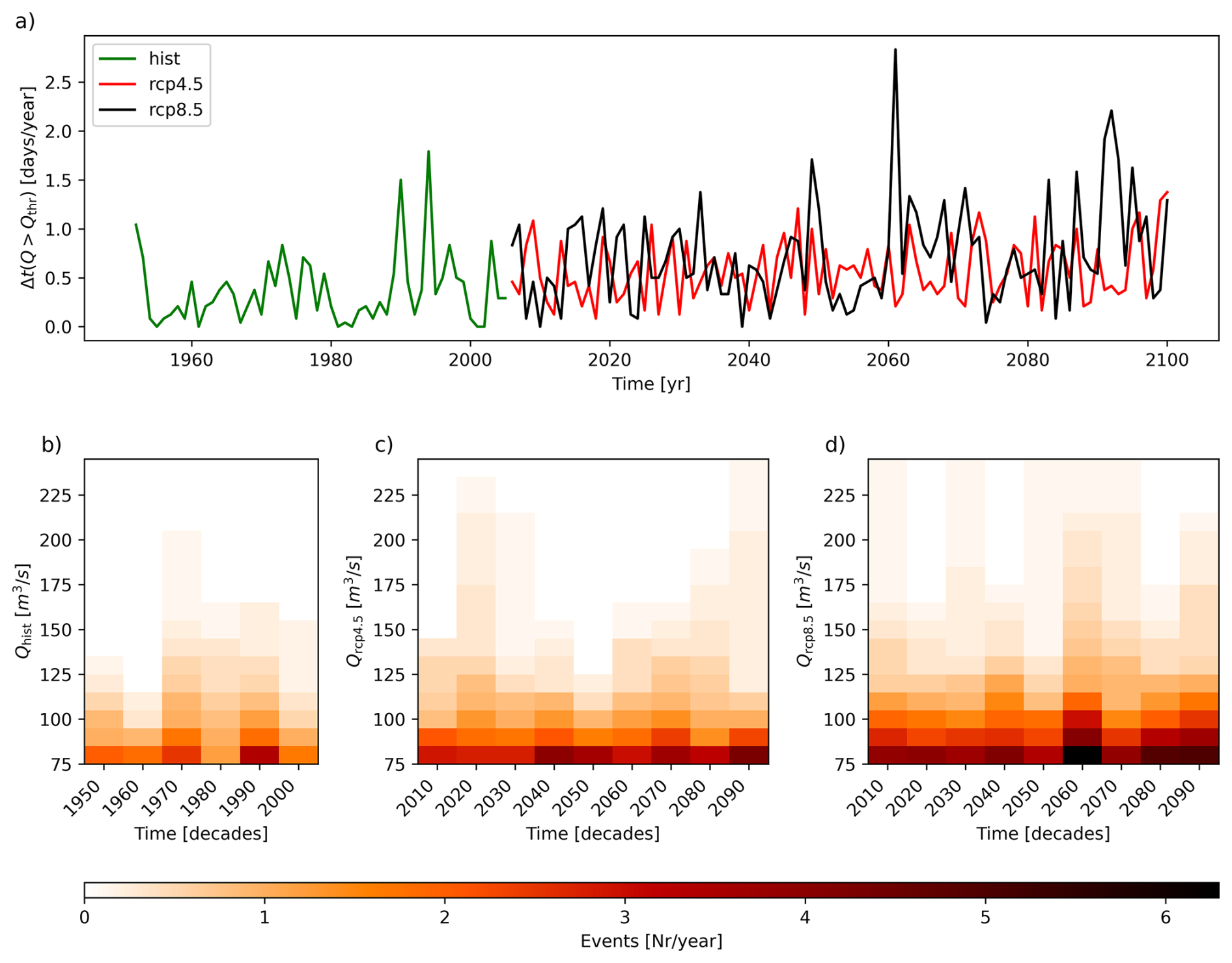
Figure 9 (a) Cumulative duration of water discharge above the 99.9 %-ile in days per year for HIST (green line), RCP4.5 (red line), RCP8.5 (black line), RCP4.5 and RCP8.5 plus the effect of RSLR (red dashed line and black dashed line, respectively), for the city of Massa. Number of events per year with peak values larger than specific values, grouped by decades for: HIST (b), RCP4.5 (c) and RCP8.5 (d).

The use of annual maxima to perform the EVA has the disadvantage of eliminating a lot of significant data. To make greater use of the time series produced, we performed two additional analyses for the city of Massa for both η_TOT(t) and Q(t). (The same analysis for the city of Villanova and Oarsoaldea is reported in the Supplement, Figs. S14 to S17). We calculated the cumulative time a variable persists over a fixed threshold, that is chosen as the 99.5 %-ile and the 99.9 %-ile of the Historical period time series for the total water level and river discharge, respectively (Figs. 8a and 9a). Furthermore, we determined the number of events per year (coloured patches) higher than specific values of η and Q (reported in the abscissa), clustering the events by decade (Figs. 8b, c, d and 9b, c, d, for Historical, RCP4.5 and RCP8.5 run, respectively).

Figure 8a shows that the increase in RSL is the main driver for the η_TOT increase for the cumulative time above a certain high level. It is also confirmed by Fig. 8b where a trend in the increase of extreme events, without the effect of RSLR, is not clearly observable.

Concerning river discharge, a slight positive trend for the cumulative time Q(t) persists above the 99.9 %-ile Historical value, is detectable (Fig. 9a). Moreover, an increase in the number of extreme events is observed, especially for the RCP8.5 scenario, even if the obtained patch is quite noisy. This can be ascribed to the fact that we used only one RCM.

The use of an empirical formula to calculate the wave runup (Atkinson et al., 2017), while avoiding us to fully simulate the dynamical swash process and getting at least the order of magnitude of runup values, introduces uncertainties due to the degree of alongshore variability of the beach or due to the reduced knowledge of the underwater bathymetry. Indeed, for the city of Massa two bathymetric surveys were available (2012 and 2016), but for Villanova the submerged part of the domain principally comes from nautical charts. Specific efforts to recover the detailed bathymetry of the area are recommended to make the resolution of the hydrodynamic domain as uniform as possible.

A potential limitation concerning the analysis of extreme events is related to compound events (Ghanbari et al., 2021; Gori and Lin, 2022). In this work we consider non-interacting storm surges and river discharges. Such a choice is aimed at simplifying the approach and having greater control on each driver of a flood event. Furthermore, the extreme value analysis of compound events leads to some difficulties and approximations related to the identification of a “compound event”. In general, focusing only on two variables, we look for large values, in one or both variables, which are temporally distant less than a specific threshold. The method to identify “compound events” varies on the basis of the different studies and scales. This aspect, together with the choice of the couple of values associated with a specific RP curve, tends to enhance the complexity and the degrees of freedom of the problem. Considering the present work as an introductory paper describing the whole modeling chain and its applications, and given the availability of continuous time series, we intend to pursue future research by focusing directly on impacts. That is, we intend to run the hydrodynamic model using as BCs the whole time series (excluding the periods where both Q and η_TOT are low), and analyze the statistical properties of the water depth as a consequence of flood events. In such a way it is possible to by-pass all the issues related to the definition and identification of compound events. Nevertheless, the availability of these long term simulated discharge time series can also be a valuable dataset for further analysis on hydrological regimes e.g. droughts.

Additionally, another issue that can be overcome in case the impact-based approach is employed, is that related to the creation of adequate synthetic boundary conditions associated with specific return periods. The choice to average the extreme events superimposed in phase at the peak can smooth out their variability, given that they show different variability ranges based on the selected city and variable (Quinn et al., 2014). Nevertheless, the obtained variability ranges do not exceed the magnitude of the associated extreme event (see Figs. S5, S6, S7 in the Supplement). It was our intent to derive a shape for the time series that is representative of the main behaviour of the analyzed variable during its rise and fall around the maximum. The derivation of a synthetic hydrograph starting from the maximum discharge is proposed by Brunner et al., (2017), where they retrieve a synthetic design hydrograph based on “the fitting of probability density functions to observed flood hydrographs of a certain flood type taking into account the dependence between the design variables peak discharge and flood volume”. They also pass through a normalization step, similar to what we carried out. However, we tried to keep a simpler approach that can be also extended to the total water levels, for which we did not find an analogous procedure.

Accounting for the tide by adding a fixed Δη_Tide to the extreme event hydrograph (Massa and Villanova), or by simulating a semidiurnal tide (Oarsoaldea) as a boundary condition, can overlook the long-term (century-scale) modifications in tidal ranges. Santamaria et al. (2017), using site specific past observations, found they are driven by meteorological, oceanographic, and hydrographic variability. The difficulty to forecast them using numerical tools partly justifies the decision not to explicitly include this aspect in the present study.

It is important to emphasize that the errors accumulating throughout the modeling chains are difficult to estimate and are the results of unavoidable approximations. Furthermore, we are running hydrodynamic simulations where the environment (e.g. buildings, structure, etc.) do not change in time, which is an unlikely circumstance. As a consequence, obtained results have to be considered as indicative of a trend rather than precise predictions of the future.

On the one hand, we are making a strong assumption, considering the surrounding environment does not change over time. On the other hand, the knowledge of specific characteristics of the analyzed area are crucial in modeling the impact of flood events. A coarse starting DEM of around 20 m resolution cannot even resolve streets and spaces between buildings, potentially blocking the flow and significantly changing the flooding pattern. These are aspects that have to be taken into account when evaluating the obtained results associated with uncertain future scenarios.

8 Conclusion and outlook

In this work we present a modeling chain to transfer synoptic scale atmospheric information to the scale of coastal cities with the goal of estimating changes in the impact of extreme riverine and coastal flood events - specifically in terms of flooded area and volume – under the RCP4.5 and RCP8.5 climate change scenarios, compared to Historical conditions. We use atmospheric data from the ALADIN63 RCM from the EURO-CORDEX dataset to drive three numerical models: WWIII for wave climate, SHYFEM for water levels, and LISFLOOD for river discharge. Model outputs are then processed to generate synthetic extreme events, which are then used to simulate coastal and riverine floods through a high-resolution hydrodynamic model (HEC-RAS). This model is specifically implemented for the domains of three coastal cities selected within the SCORE Project: Massa (Italy), Vilanova i la Geltrù, and Oarsoaldea (Spain). Wave climate data are further used to calculate wave runup, which is combined with water levels to determine total water levels η_TOT.

The extreme value analysis of total water levels η_TOTand river discharge Q reveals both increase and decrease in RCP4.5 and RCP8.5 extremes compared to Historical extremes, depending on the different locations, with larger uncertainties associated with high extreme values and longer-term projections (2051–2100). The increase/decrease in flooded volume is not necessarily related to increase/decrease in extremes but it depends on relative sea-level rise RSLR and to specific local features of each coastal city.

Massa is particularly vulnerable to RSLR, which facilitates the inland propagation of coastal floods, increasing the water volume up to 68 %. Additionally, RSLR hinders river flow into the sea, exacerbating riverine floods and potentially doubling water volume. This is further compounded by an increase in future extreme river discharge (ranging from +2.9 % to +70 %), especially under the RCP8.5 scenario. In contrast, Vilanova i la Geltrù is not significantly affected by storm surges due to its geomorphic structure, whereas the riverine extreme floods tend to generally increase in the future according to RCP4.5 and RCP8.5 (up to +27.5 % for peak river discharge and +33 % for water volume). Oarsoaldea, on the other hand, is well protected against storm surges and the flood extension appears to be relatively insensitive to the differences between Historical, RCP4.5 and RCP8.5 scenarios. Riverine floods in Oarsoaldea show a decrease in extent for the 100 years RP but slightly increase for the 25 years RP in the 2051–2100 timeplay. These results reflect the complex interplay between extreme events and RSLR.

This study highlights the importance of employing high resolution modeling, as local characteristics significantly influence flood impacts and the analysis of the effects of future extreme events.

Future developments include the use of long-term time series of η_TOT and Q to continuously force the hydrodynamic model, excluding periods associated with low values. This impact-based approach can potentially replace the need for EVA for different events, including compound ones and enables a direct analysis of their interaction on the ground, providing a statistical assessment of water depth, flood extent and water volume time series.