Quantifying the attributable impact of the February 2018 sudden stratospheric warming on mortality in the Nordics and United Kingdom

Sudden stratospheric warming (SSW) events take place well above the Earth's surface, but can nonetheless trigger extended periods of cold surface weather in Europe, with potential consequences for public health. While previous work has established statistical links between SSWs and increased winter mortality, quantitative attribution of deaths to specific SSW events remains limited, particularly across different regions and data resolutions. This study presents a counterfactual attribution framework that combines exposure-response curves with stratospherically nudged ensemble forecasts to robustly attribute excess mortality to the February 2018 SSW event and its associated cold surface anomalies. We analyse mortality in various UK regions as well as three Nordic countries using a combination of daily, weekly and monthly aggregated mortality datasets. Exposure-response curves are derived using both distributed lag nonlinear models (DLNMs) and a simpler binning-based approach, allowing evaluation across varying temporal resolutions and data constraints. We find that while the Nordic countries experienced the strongest post-SSW temperature anomalies, the attributable mortality risk impacts are mostly found in the UK. This is explained by the steepness of the cold branch of the exposure-response relationship in southern UK regions, likely reflecting lower population-level adaptation to cold weather. Our ensemble-based attribution framework suggests that several hundred expected deaths in England and Wales and a combined total of a few hundred in the Nordics can be attributed to the 2018 SSW, with substantial uncertainty arising from both the estimated exposure-response relationships and the spread between forecast systems. Comparing DLNM and binning approaches across daily, weekly and monthly input data, we find that the resulting estimates agree in sign and order of magnitude, which supports the use of coarser data where higher resolution is unavailable while making the associated structural uncertainty explicit. The regional variation in exposure-response characteristics further highlights the need to consider both meteorological hazard magnitude and societal vulnerability. Beyond mortality, the framework is applicable to other societal impacts of extreme weather, providing a flexible and interpretable tool for retrospective attribution and climate risk assessment.

1 Introduction

Severe weather events involving temperature extremes pose significant public health challenges. A substantial focus of existing literature lies on health impacts of heat extremes, while the total amount of excess deaths attributable to cold anomalies can be several times higher (Gasparrini et al., 2015). This is because even moderate drops in temperature can sharply elevate health risks (e.g., Analitis et al., 2008; Sarofim et al., 2016; Walkowiak et al., 2024). For instance, a study by Zeka et al. (2014) has shown that a 1 °C decrease in winter maximum temperature in Ireland can correspond to about a 6.4 % increase in all-cause mortality. However, epidemiological research indicates substantial regional difference in the impacts of temperature anomalies on mortality risk, depending on the general adaptation to cold due to climatological temperature values, socio-economic factors like access to adequate heating or demographic differences (The Eurowinter Group, 1997; Kysely et al., 2009; Hajat et al., 2014; Mistry et al., 2022). Correspondingly, predicting the actual impacts of weather and climate anomalies has thus become a topic of increasing interest to allow for more effective public health planning and targeted mitigation measures (Lowe et al., 2015; Pyrina et al., 2025).

A key phenomenon that has been linked to prolonged periods of increased risk of cold extremes in Europe are sudden stratospheric warming (SSW) events (Kolstad et al., 2010; Kretschmer et al., 2018; Huang et al., 2021). These events involve a rapid increase in polar stratospheric temperatures and a disruption of the stratospheric polar vortex (see review by Baldwin et al., 2021). Despite being located in the stratosphere, the associated circulation anomalies can propagate downward to the surface and affect tropospheric weather patterns (Baldwin and Dunkerton, 2001). The tropospheric response to SSWs typically includes a tendency for negative phases of large-scale circulation patterns like the Arctic Oscillation (AO) or the North Atlantic Oscillation (NAO). These circulation anomalies then often lead to colder-than-average conditions and an increased likelihood for cold spells across Eurasia, including Northern Europe and the United Kingdom. Due to the generally long time scales of the stratosphere (Baldwin et al., 2003), the surface impacts can last for several weeks to months (also referred to as subseasonal time scales) and hence SSWs offer unique opportunities for improved forecasts (Kautz et al., 2020; Domeisen et al., 2020; Büeler et al., 2021; Spaeth et al., 2024). As we will show, these long time scales also provide a unique opportunity to obtain meaningful attribution insights from temporally aggregated impact data, which would be much less suitable for short-lived weather extremes.

The February 2018 SSW is an excellent example: this event has been shown to be associated with severe cold conditions and anomalous snowfall across Northern Europe and the UK, widely termed the “Beast from the East” (Greening and Hodgson, 2019; King et al., 2019; Overland et al., 2020). In the present study we use this 2018 event as case study, to attribute potential excess mortality to the occurrence of an SSW. Figure 1 shows the surface temperature anomaly following the 2018 event and the composite mean over many SSWs for the United Kingdom and the Nordic countries Norway, Sweden and Finland (see Sect. 2 for details of the data and SSW dates used). It can be seen that the surface temperature response, while overall negative and robust, shows clear spatial patterns. In particular, northern Europe typically shows substantially stronger temperature anomalies compared to, e.g., the United Kingdom.

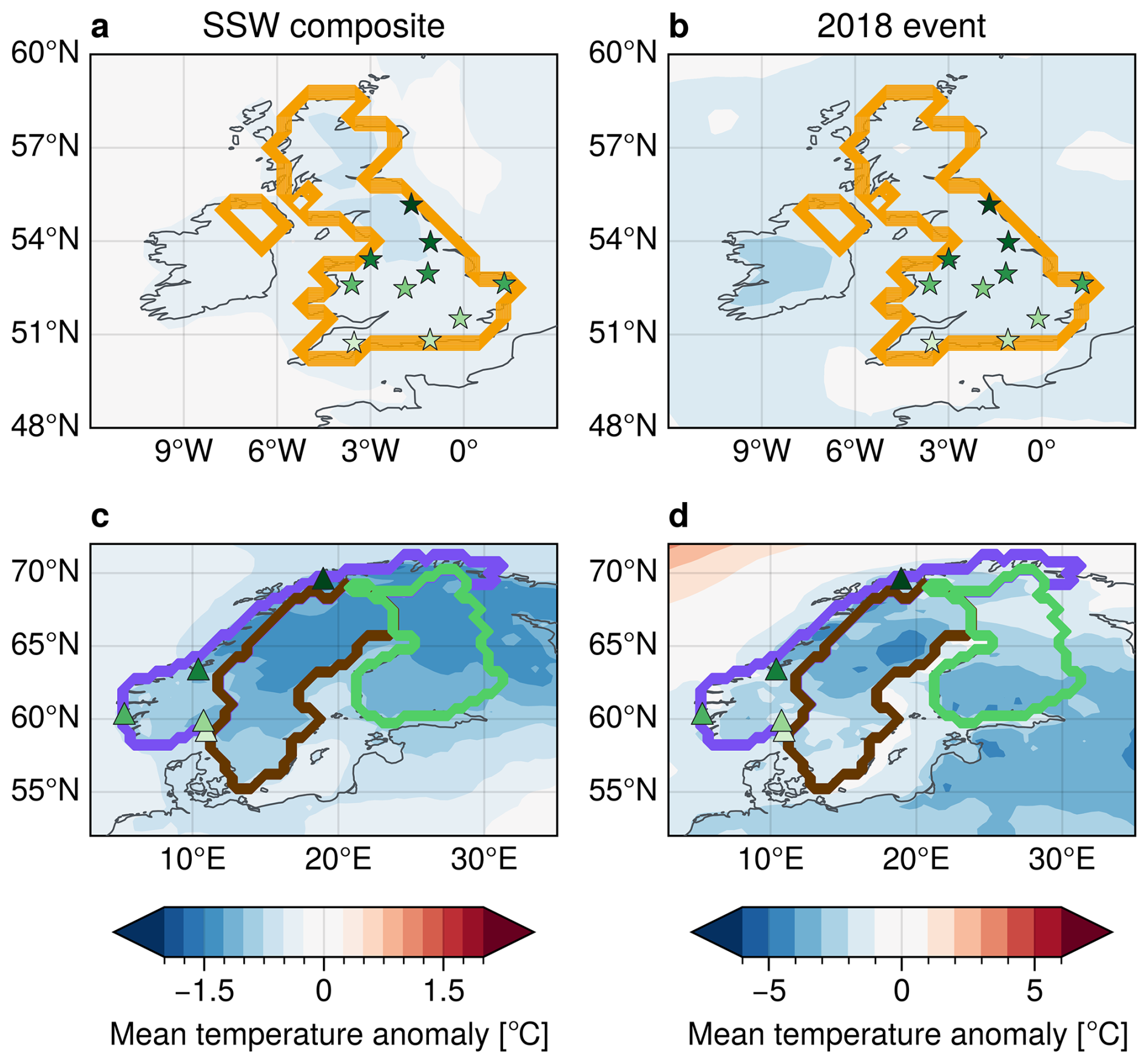
Figure 1 Climatological anomaly of 2 m temperature for (a, b) the United Kingdom and (c, d) Northern Europe in re-analysis data. Panels (a) and (c) show a composite mean averaged over 30  d following 41 SSW events between 1960 and 2023, panels (b) and (d) show the average over 30  d following the 2018 SSW (note different colour scales). Markers show the locations used as representative for different regions in the UK and Norway (see Table 1). Coloured contour lines show the outlines of the countries of interest (United Kingdom, Norway, Sweden and Finland).

Recent studies directly link SSW-induced cold spells to significant mortality increases. For instance, analyses of UK mortality following major SSW events reveal approximately 620 excess deaths attributable to these events, on average (Charlton-Perez et al., 2021). Such findings underscore the tangible public health consequences of stratospheric variability. Yet, quantitative assessments of mortality impacts related explicitly to SSW events remain limited, particularly in terms of regional differences of these impacts. This geographical knowledge gap, in addition to the long-leadtime forecasting potential of SSW events, motivates the need for broader regional assessments of the socio-economic impacts of SSWs to enhance targeted preparedness.

Quantifying cold-related health impacts typically relies on statistical models linking an exposure variable (like temperature) and a response variable (like mortality), e.g., via exposure–response curves (Huang et al., 2012; Gasparrini and Armstrong, 2013; Wang et al., 2016; Mistry et al., 2022). A widely used methodology to compute such exposure-response curves utilises Distributed Lag Non-linear Models (DLNMs) due to their capability to capture both nonlinear and delayed temperature effects (Gasparrini et al., 2011; Gasparrini and Armstrong, 2013). However, to accurately account for lag-relationships to short-term variations, DLNMs require high-temporal-resolution data (often daily), which may not be consistently available across different regions or periods.

Methods to apply DLNMs to temporally aggregated mortality data have been developed in recent years (Basagaña and Ballester, 2024). In the present study we use daily DLNMs where daily data are available, weekly DLNMs where the record is long enough to support them, and complement both with a simple binning approach that can be applied uniformly across all our datasets. Comparing these approaches across regions and temporal resolutions allows us to quantify how strongly the attribution results depend on the choice of exposure-response model and on the resolution of the input data. The fact that qualitatively consistent conclusions emerge across most of these combinations gives additional confidence in the overall findings.

To systematically quantify the mortality impacts of the 2018 SSW, we leverage ensemble simulation experiments from the Stratospheric Nudging and Predictable Surface Impacts (SNAPSI) project (Hitchcock et al., 2022). SNAPSI provides coordinated model experiments where the zonal-mean strength of the polar vortex is nudged either towards observed conditions (thus ensuring the presence of an SSW) or towards climatology (effectively removing the SSW signal). Comparing these two scenarios enables a counterfactual attribution of surface impacts and associated mortality to the SSW event, analogous to an exposed versus unexposed design in epidemiology, but with the exposure (the SSW) explicitly controlled in the model experiments. The use of such ensemble simulations over simple re-analysis composite further supports the feasibility of attribution studies and impact analyses when only coarse temporal impact datasets are available (e.g. weekly scale).

The structure of this paper is as follows. Section 2 gives a detailed overview of the utilised datasets and numerical models. In Sect. 3 we then introduce the general framework to assess attributable impacts of SSW events on mortality via exposure-response curves and nudged ensemble simulations. We further test the sensitivity of this framework with regard to different exposure-response model approaches and temporal resolution of the input mortality data. Afterwards, Sect. 4 applies the framework to assess the mortality impacts of the 2018 SSW for the UK and Nordics, with particular focus on the regional differences and relative risks compared to the spatially non-uniform temperature signal (see Fig. 1). Finally, Sect. 5 briefly summarises and discusses the main conclusions of this study.

2 Data and numerical models

The attribution analysis presented in this study requires three types of datasets. First, we need observational temperature data covering a sufficiently long historical period to robustly construct exposure-response relationships between temperature anomalies and mortality risk. Second, corresponding mortality data for the same historical period is required. Finally, ensemble model forecasts of the 2018 SSW event is essential for quantifying the mortality impacts directly attributable to this stratospheric event. The following subsections detail each of these datasets, including their sources, spatial and temporal resolutions, and covered periods.

2.1 Re-analysis data

The ERA5 re-analysis dataset (Hersbach et al., 2020) of the European Centre for Medium range Weather Forecasts (ECMWF) is used as the representation of atmospheric state. In particular, we use 2 m temperature (t2m) provided on a 0.5° × 0.5° regular grid. All analyses are based on daily means, computed from 6-hourly data. Throughout the manuscript we use the period 1 January 1960 to 31 December 2018 as a reference to compute daily climatological means (smoothed with a 31 d running mean, to reduce high frequency sampling variability) and corresponding anomalies. For analyses where mortality is only given in a shorter period, we accordingly use fields and anomalies within the overlapping period. Sudden stratospheric warming event onset dates are based on the SSW compendium described in Butler et al. (2017).

Note that the temperature (and mortality) datasets used in this study potentially include long-term trends, e.g., due to climate change. We do not explicitly remove these trends before processing the data (cf. Fig. 3). However, some of the methods we use (specifically the DLNM, see Sect. 3.1) uses a spline-interpolation to remove seasonal variations in the data. This will likely also remove part of any long-term trend included. Other methods (like the binning approach, see Sect. 3.2) do not remove any trends or seasonal variability. As we will show later, the good agreement between these two methods suggests that long-term trends do not affect our conclusions.

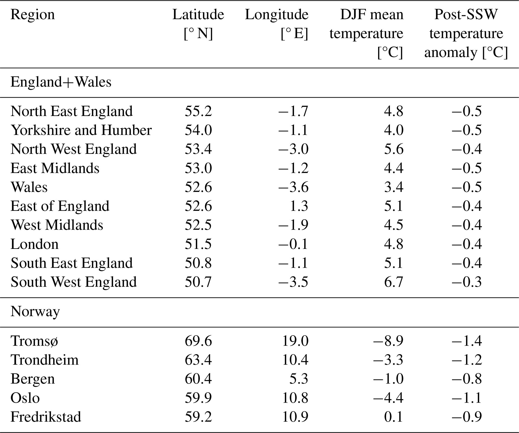
To define temperature time series for various regions of interest we use two approaches. For country-level analyses, we use spatially averaged near-surface temperature fields. While aggregation methods like population-weighted temperature series can provide a closer representation of individual exposure, their construction requires additional demographic datasets and assumptions (e.g. spatial re-gridding) that introduce further uncertainties. Given the spatial coherence of SSW-related temperature anomalies over large regions (Figs. 1 and 2), and as our attribution relies on differences between nudged and control ensemble simulations rather than absolute temperature levels, we expect spatially averaged temperatures to provide a reasonable approximation for country-scale impacts. On the city and region level, we use a single representative point for the respective region. This point is chosen to be rather central within a county, and ideally close to a larger city, to obtain the strongest connection to potential mortality impacts. Using representative single points for regional signals can be justified due to the generally large scale surface temperature structures within the ERA5 and model datasets (see Figs. 1 and 2). Table 1 shows the choice of representative points for the different regions studied within Norway and the United Kingdom.

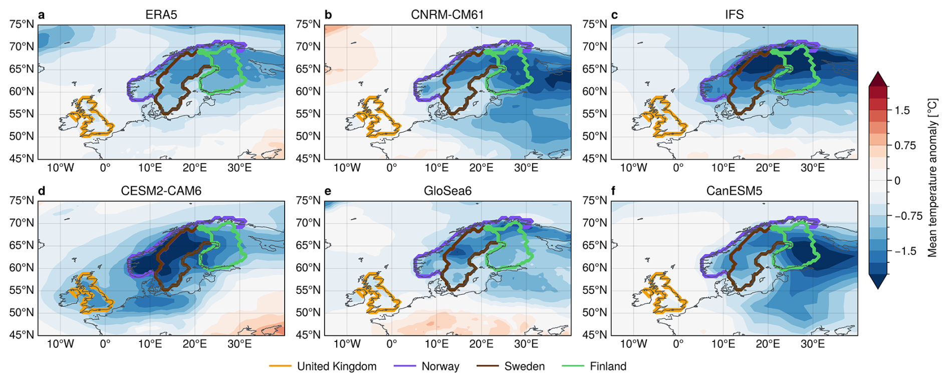
Figure 2 Composite mean anomaly of 2 m temperature for part of Europe in (a) re-analysis data and (b–f) model simulations. Anomaly in re-analysis are computed w.r.t. climatology, anomalies for models are computed as difference between nudged and control experiments. All panels show the average over 30 d following the 2018 SSW onset. Coloured contour lines show the outlines of the countries of interest.

Table 1 Climatological and post-SSW characteristics for different regions in the UK and Norway. Shown are the latitude/longitude points used to extract time series for the individual regions, the climatological DJF-mean temperature and the composite mean temperature following 41 SSW events (1960–2023).

2.2 Mortality data sources

Health impacts in this study are quantified in terms of excess mortality. Here, we use all-cause mortality in absolute numbers, typically collected from local health authorities and health institutions. The mortality data used in the present study was obtained from various sources, with different temporal and spatial resolutions and covered periods; see Table 2. While higher-resolution mortality series may exist in several countries, they are not always publicly available, harmonised across regions or readily accessible for multi-country attribution studies, motivating the use of multiple datasets with varying resolution in this paper.

Table 2 Mortality datasets used in this study for the countries United Kingdom (UK), Norway (NO), Finland (FI) and Sweden (SE). Last access for all web pages cited in this table: 3 November 2026.

2.3 Model experiments

We use a set of ensemble re-forecasts conducted as part of the Stratospheric Nudging And Predictable Surface Impacts (SNAPSI) project. In particular, we use runs performed with 5 different modelling systems, all initialised on 25 January 2018 (with observed SSW onset on 12 February). The SNAPSI simulations include a nudging of the stratospheric zonal mean zonal wind and temperature to either the observed evolution during that time period (“nudged” experiment) or a climatological evolution (“control” experiment). The nudging strength tapers smoothly with pressure, transitioning from zero below 90 hPa to full strength at 50 hPa following a cubic profile, thereby minimising edge effects near the tropopause. Each experiment is run with 50 ensemble members. Correspondingly, in these model simulations all members either exhibit an SSW (in the nudged runs) or none of the members exhibit an SSW (in the control runs). Computing the difference between nudged and control experiments therefore provides an explicit counterfactual framework, in which the presence or absence of the SSW is controlled across otherwise identical ensemble members. This allows us to determine a statistically robust estimate of the influence of the SSW on the troposphere, independently of intrinsic tropospheric variability.

Note that the SNAPSI project further provides simulations initialised on 8 February, which we will not analyse in this study. While we do expect our results to be qualitatively similar for both initialisation dates, we focus on the earlier initialisation to ensure that the developing SSW does not affect the ensemble evolution and both nudged and control runs can be seen as “plausible futures”. For more information about the model setups, see Table 3 and Hitchcock et al. (2022).

Voldoire et al. (2019)(ECMWF, 2025)Richter et al. (2022)Williams et al. (2018)Swart et al. (2019)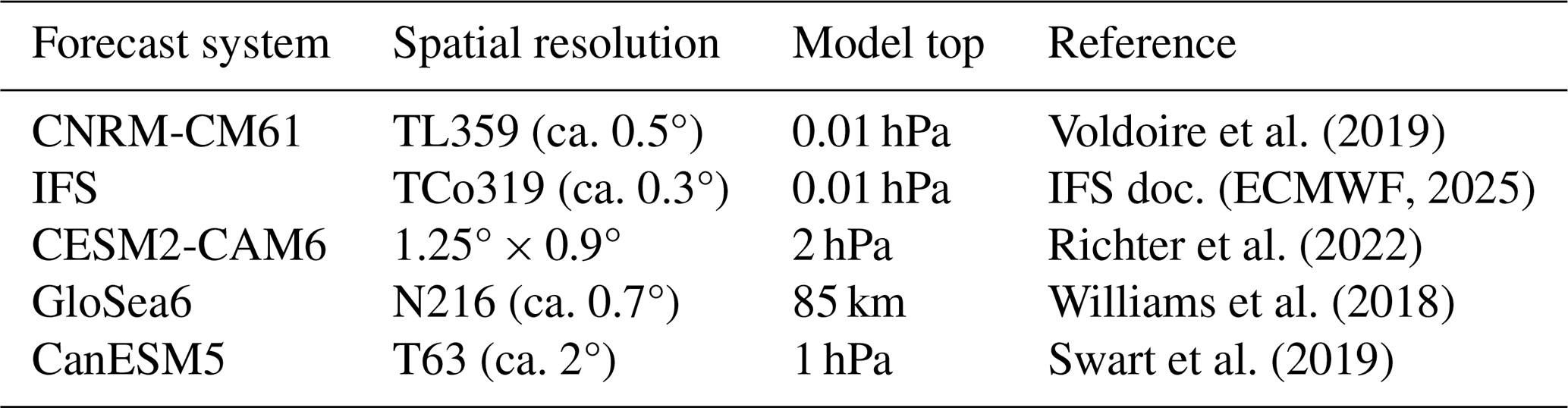

Table 3 Details of model setups within the SNAPSI project.

The SNAPSI model experiments show a reasonable signature of SSW downward impact in terms of surface temperature field. Figure 2 compares the model surface temperature anomaly (as nudged-minus-control) to the climatological anomaly in re-analysis. All model runs show a pronounced cold anomaly over northern Europe, clearly covering Norway, Sweden and Finland. In some models this cold anomaly extends westward up to the UK, although other models show no or very weak anomalies here (consistent with observational variability). The model run with CESM2-CAM6 shows particularly strong temperature anomalies that extend very far west. However, note that this setup uses a rather low model top (2 hPa), which could explain the overestimation of the downward response due to misrepresentations of stratospheric processes.

The good overall agreement between model signals and re-analysis gives confidence that this setup is suitable to study the potential mortality impact of the 2018 SSW in these regions.

3 Methodology

3.1 Exposure-response curves from DLNMs

We quantify mortality attributed to SSW-related cold anomalies using a distributed lag non-linear model (DLNM), based on the R package discussed in Gasparrini et al. (2011). Various authors have previously used DLNM approaches to link temperature extremes to mortality impacts (Guo et al., 2016; Vicedo-Cabrera et al., 2018; Lo et al., 2022). The DLNM is essentially an extension of quasi-Poisson regression that characterises the temperature-mortality relationship, controlling for potential external effects like long-term trends and seasonal cycles (as natural cubic spline of time with 8 degrees of freedom per year), as well as an indicator for day-of-week. Temperature exposure is modeled with a 21 d lag period and five knots placed at the 10th, 25th, 50th, 75th, and 90th percentiles of the input data. These knots are points in the predictor distribution where the DLNM fit can change the properties of the underlying basis function and is hence used to determine the degrees of freedom and of the resulting function. Although we did not find a knot range between 3 and 7 to give substantially different results, the knot placement and density can in principle lead to over- or underfitting in different regions of the exposure-response curve.

Output of the DLNM is an overall cumulative relative risk (RR) curve, estimated with respect to the minimum mortality temperature (MMT). The MMT is identified as the temperature associated with the lowest mortality risk for a given location. We use this curve within the standard framework for temperature-attributable mortality (Gasparrini and Leone, 2014), in which the attributable number of deaths AN is the difference between the expected deaths in a world with the signal present and those in a reference world without it. In the classical setting the reference state is the MMT and, with n_MMT the death count expected at the MMT and RR_obs the relative risk at the observed temperature, the attributable number can be computed as

$$\begin{array}{}\text{(1)}& \begin{array}{rl}\text{AN}& =n_{\mathrm{MMT}}{\text{RR}}_{\mathrm{obs}}-n_{\mathrm{MMT}}=n_{\mathrm{MMT}}\left({\mathrm{RR}}_{\mathrm{obs}}-\mathrm{1}\right)\\ & =n_{\mathrm{obs}}{\displaystyle \frac{{\text{RR}}_{\mathrm{obs}}-\mathrm{1}}{{\text{RR}}_{\mathrm{obs}}}}=n_{\mathrm{obs}}\text{AF},\end{array}\end{array}$$

where n_obs = n_MMTRR_obs is the observed death count. The rightmost expression is the usual product of the observed deaths with the attributable fraction AF.

In our study, however, the reference state does not correspond to the MMT but to the SSW-free control ensemble, which can itself be at elevated or reduced risk. Since both ensembles describe the same population on the same calendar dates, n_MMT is identical in the two worlds and

$$\begin{array}{}\text{(2)}& \text{AN}=n_{\mathrm{MMT}}\left({\text{RR}}_{\mathrm{n}}-{\text{RR}}_{\mathrm{c}}\right)=n_{\mathrm{obs}}{\displaystyle \frac{{\text{RR}}_{\mathrm{n}}-{\text{RR}}_{\mathrm{c}}}{{\text{RR}}_{\mathrm{obs}}}},\end{array}$$

with RR_n and RR_c the relative risks corresponding to the temperatures simulated in the nudged and control experiments. The attributable fraction is thus evaluated against the control ensemble rather than against the MMT.

Both forms (Eqs. 1 and 2) require an estimate of n_MMT, on which the quantitative result depends to a large extent. The rightmost form of Eq. (2) estimates it from observed deaths during the event, which requires RR_obs and therefore either re-analysis temperatures (which may be different with respect to the model) or simulated temperatures from the nudged experiment (which carry model error). In the present study, we instead estimate n_MMT as the mean death count within a ±1 °C bin around the MMT over the full period of the respective mortality record, assuming that model deficiencies are small for climatological averages. This route requires no observed mortality or temperature contemporaneous with the period evaluated, and can therefore also be applied unchanged to counterfactual or projected climates (as, e.g., in Gasparrini et al., 2017). Different estimates of n_MMT can differ, depending on the method of choice: over the 30 d following the 2018 SSW onset, the observation-based estimate exceeds our climatological value by about 18 % in South East England and falls below it by about 8 % in London. A priori it is not clear that either route is more accurate, and differences of this size are comparable to or smaller than other uncertainties in our framework, in particular the spread in simulated temperatures between forecast systems (Sect. 4). Bounds for the 95 % confidence interval of mortality estimates are also derived from the model package.

Figure 3 Mortality versus temperature for London. The gray line shows the exposure-response curve computed using a distributed-lag non-linear model (DLNM). Shading indicates the 95 % confidence interval. Dots show daily death counts versus temperature on that day for the period 1981–2018, with colours representing the season. Horizontal dashed line indicates the baseline mortality corresponding to the MMT.

Figure 3 illustrates the estimated temperature-mortality exposure-response curve compared to the direct temperature and mortality relationship on the same day (i.e. no lag), for winter, summer and shoulder-season days. It can be seen that much of the temperature-mortality relationship follows the general behaviour of the seasonal cycle, despite the DLNM controlling for seasonal variability. Note that the climatological spread in death counts (e.g. as standard deviation) for a fixed temperature bin also follows a similar qualitative shape (not shown), with minimum spread near the MMT and increasing spread for lower and higher temperatures.

Generally, the DLNM-derived exposure response curve captures an increased risk for cold and warm extremes. The confidence intervals in Fig. 3 are narrow, reflecting the large number of daily death counts entering the fit at this level of spatial aggregation. Two sources of uncertainty are worth distinguishing here. The first is the sampling uncertainty of the fitted curve, which is indeed small. The second is the structural uncertainty about the functional form in temperature ranges that are only sparsely sampled: for regional extremes (below ca. −5 °C or above ca. +25 °C in the case of London) the shape of the curve is constrained by few observations and is partly inferred from the more moderate range through the spline basis. The confidence bounds returned by the model quantify the former but not the latter, and we use the comparison between different exposure-response models in Sect. 3.2 as an indication of the latter. Overall, the structural uncertainty remains large in these extreme ranges and it is not clear if the DLNM-derived curve is necessarily the best description of the underlying data.

3.2 Robustness to model assumptions and data resolution

In Sect. 3.1 we described how to obtain a exposure-response curve from using a DLNM. However, DLNMs are relatively complex and require a choice and optimisation of various model parameters (knots, control variables), as well as high-temporal-resolution data (often daily), to capture the lag-relationships. For some regions, we found that such daily mortality data is not available.

In this section we therefore investigate a simpler approach to obtain an exposure-repsonse curve, based on a binning method. Essentially, we define temperature bins with width of 2 °C for the given range of values within a certain dataset (e.g. for London). We then average both mortality and temperature (extracted on the same day, i.e., with no lag) within each bin to obtain a single function of death count for a given temperature. To apply an additional smoothing, we fit a 3rd-over natural-spline to the resulting temperature-mortality curve, with knots at the 25th, 50th and 75th percentile of the binned data. Note that binning before fitting is not equivalent to fitting a spline directly to the unbinned data: it assigns equal weight to each temperature bin rather than to each observation, increasing the influence of the sparsely sampled tails relative to the densely populated range near the MMT. This is deliberate, since the tails are the region of interest for cold attribution, but it also makes the fit more sensitive to noise there, as reflected in the wider bootstrap intervals at the edges of the curves. Uncertainty bounds for the resulting exposure-response curve are computed via bootstrapping with 1000-draws from the original input data pool before applying the binning approach. (Note that we use the same bins, based on the original dataset, for each bootstrapping sample, for practical reasons.) The purpose of this approach is not to propose an alternative method to DLNMs as a general epidemiological standard, but to provide a transparent and flexible mapping from temperature to expected mortality that can be applied uniformly across all our datasets and to give an estimate of structural model uncertainty in our impact attribution framework. In addition, we find overall agreement across the model approaches in terms of sign and order of magnitude in expected risk and death cound increase associated with the 2018 SSW, giving confidence in our findings and drawn conclusions. We stress that the binning approach is not free of methodological choices either: the bin width acts as a complexity parameter in the same way as the number of spline knots in a DLNM and the treatment of lags and the decision whether and how to control for seasonality or other confounders remain free choices. In particular, the binning approach as applied here does not control for seasonality, day of week or long-term trends.

Figure 4 Exposure-response curves for London based on input data as (a) daily, (b) weekly and (c) monthly average. Red dots show death counts versus temperature distribution at the corresponding temporal resolution. Lines show the exposure-response curves using the DLNM or binned-data approach, with shading indicating the 95 % confidence interval. The daily DLNM line is the same in every panel and is based on daily data only. Panel (b) additionally shows a DLNM exposure-response curve based on weekly data. Horizontal dashed lines indicate the baseline mortality corresponding to the MMT.

Figure 4a illustrates that the exposure-response curves obtained from binning and DLNM approaches are generally in good agreement, with 95 % confidence intervals overlapping for most sampled temperatures. Discrepancies are mostly present for extreme temperatures, where the underlying data uncertainty becomes large and it becomes difficult to argue that either of the models is a more accurate representation of the corresponding relationship. We note that in some regions the exposure-response curves flatten or show non-monotonic behaviour at very cold temperatures. These features occur primarily in temperature ranges with very limited data coverage and reflect statistical uncertainty rather than robust signal. While multivariate meta-analytic DLNM approaches that pool spline parameters across locations can stabilise such extremes (Sera and Gasparrini, 2022), applying these methods would substantially increase methodological complexity and is beyond the scope of the present study. Importantly, the consistency of estimated mortality impacts across both DLNM and binning approaches suggests that these local curve features do not materially affect our attribution results.

A main advantage of the binning approach is that it can be easily applied to almost any input dataset, including lower temporal resolution data. Figure 4b and c show the resulting exposure-response curves for London based on weekly and monthly input, respectively. Note that the daily DLNM-derived curve is computed from daily input data and repeated in every panel for reference. DLNMs can also be applied directly to temporally aggregated records (Ballester et al., 2023; Basagaña and Ballester, 2024) and we have applied a weekly DLNM approach following Ballester et al. (2023) to estimate the temperature-death relationship within the different UK regions (e.g. Figs. 4b). However, we use the binning-based approach alongside DLNM approaches to assess robustness to model choices and additionally in situations when DLNM approaches are not feasible, like when only coarser temporal aggregation is available or the record length is too short (e.g. for Sweden). While the overall temperature range narrows for aggregated data (since extreme temperatures become less frequent) the general shape of the response curve remains stable. Notably, the cold branch becomes steeper, which likely reflects a statistical compression effect: extreme daily values that drive mortality risk are smoothed out in aggregation, causing the same deaths to be concentrated into narrower temperature bins. However, we do find a general consistency between different model approaches (DLNM vs. binning) and temporal data resolutions (daily to monthly). This robustness across approaches and datasets does not only hold for London, but also other regions within the UK and the Nordics, like Oslo (Fig. S1 in the Supplement).

Figure S2 extends this comparison of methods and temporal resolutions to Finland and Norway and to the weekly DLNM. Agreement between DLNM and binning curves is good over the densely sampled part of the temperature distribution in all cases, while differences grow in the sparsely sampled tails and between temporal resolutions. For Norway, the difference between the daily and weekly DLNM curves exceeds that between the DLNM and binning curves at either resolution, indicating that the temporal resolution of the input data is at least as important as the choice of exposure-response model. We therefore present results from several approaches throughout, rather than a single best estimate, so that this structural uncertainty remains visible.

The overall consistency and robustness of our analysis gives confidence in the methodology and supporting the framework’s utility in data-limited settings.

As one of the main arguments for the use of DLNMs is often given the fact that it incorporates a lag-relationship, to capture delayed effects of short-term variations in the exposure variable. In principle, we can also include a lag-relationship in our binning approach. Figure 5 shows the sensitivity of the binning-derived exposure-response curves compared to the DLNM versions for three example regions in the UK. Here the lag is used to link the temperature on day t to the accumulated death count between days t and t + lag, similar to what is typically done within the DLNM (recall that we use a lag of 21 d within our DLNM). First, it can be seen that the cold branch of the exposure response curve stays robust, with no major dependency on the chosen lag for any of the three regions. For the examples of North West England and London (Fig. 5a and b), the binning-derived cold branches are in good agreement with the exposure-response curve obtained via the DLNM. For the example of South West England (Fig. 5c) the binning-derived curves stay robust with respect to varying lags, but deviate from the DLNM-derived curve for extremely low temperatures (below about 0 °C). However, the data coverage for these extremely low temperatures is very low and hence the exposure-response curve will strongly depend on the details of the underlying model like fitting parameters.

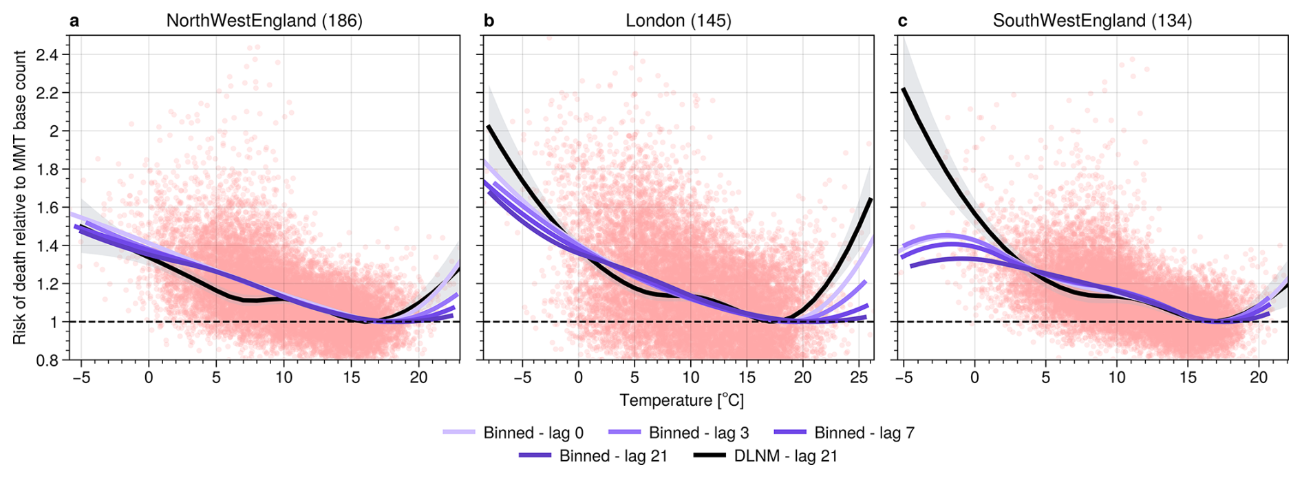
Figure 5 Exposure-response risk curves for three different regions in England based on daily data. Dots show the distribution of mortality risk versus temperature, with risk computed as death count normalised by the MMT base count (shown in brackets) and using no lag in all panels. Lines show the exposure-response curve based on the DLNM or the binning approach. The DLNM uses a lag of 21 d, for the binning approach is shown for varying lag between 0 and 21 d.

Although a decreasing mortality risk at extremely low temperatures is not epidemiologically expected, these features occur in temperature ranges with very sparse sampling and are therefore weakly constrained statistically. While one might argue that a decreasing mortality risk for extremely low temperatures is not epidemiologically expected, it is not a priori clear which of the models (DLNM or binning approach) gives a more appropriate simplified representation of the underlying data distribution. The deviation between the curves derived via different approaches arise to some extent from a “model error”, which acts in addition to the “sampling error” that arises due to limited sampling (e.g. as indicated by shading in Fig. 4. We therefore interpret differences between the DLNM and binning curves at these extremes primarily as a manifestation of limited data coverage and model structural uncertainty, rather than as a robust signal.

The warm branch of the binning-derived curves only show a steep increase with increasing temperatures for small or vanishing lags. In the case without lag the binning-derived curve closely follows the DLNM-derived curve while it stays rather flat and close to a relative risk of 1 when choosing larger lags. This behaviour could be explained as heat-related extremes are typically coupled to mortality on very short time scales Gasparrini and Armstrong (e.g. 2011). A heatstroke on a particularly hot day, for example, will lead to death on the same or the following days, but will hardly lead to a death 3 weeks after. Without controlling for long-term variability (as done in the DLNM), this could smooth-out the short-term effect of heatwaves when using long lags. Cold-related deaths, however, often occur from persistent cold temperatures, that sometimes do not necessarily require large magnitudes (see, e.g., Gasparrini et al., 2015; Wang et al., 2016; Keatinge et al., 2000). Hence, the cold branches of the curves stay less affected by temporal aggregation.

4 Results

4.1 Demographic and regional variations in mortality risk for the UK

Before quantifying SSW-attributable mortality impacts, we first summarise key demographic and regional features of the estimated exposure–response relationships. Mortality risk for cold anomalies is often a highly non-linear function of various parameters besides temperature itself. For example, demographic characteristics like age can strongly affect the impact of temperature anomalies on mortality. While younger people are usually very resilient to cold, older people can be highly vulnerable. However, the death risk for the younger population can still increase substantially for extreme cold values.

Figure 6 shows that, for example, the risk of death for people 65 years or younger increases by almost 50 % in London, when temperatures reach −5 °C (compared to the MMT value). For certain regions, like North West England, the difference in increased risk during cold periods is only marginally smaller for people below 65 years, compared to people above 65. This indicates that the impact of cold spells (e.g. following SSWs) is not restricted to the oldest parts of the population. In fact, depending on demographics and economic development, younger parts of the population can be even more vulnerable (Kysely et al., 2009).

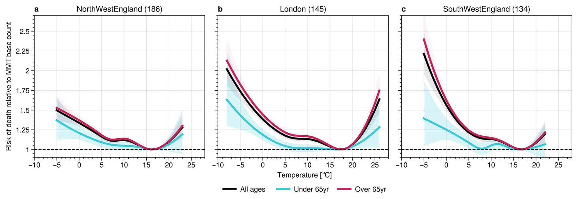
Figure 6 Exposure-response curves for mortality risk as function of temperature for three different regions in the UK. Curves show the mortality risk for all ages, and below/above 65 years. Shadings indicate the 95 % confidence interval. Numbers in brackets give the baseline mortality count at MMT.

In general, we find the cold branch of the mortality risk curve to be much steeper in some regions compared to others. In particular, there is a tendency for UK regions further south to be associated with much steeper curves than regions further north (see Fig. 7). This behaviour could be explained by the fact that northern regions are more used to experiencing cold conditions and their populations are therefore “better adapted” to cold periods. Demographic differences between regions may also play a role. Although it might be surprising to see such a clear gradient on a regional scale, this finding is consistent with results of other authors, who showed that European countries with higher climatological temperatures are usually more vulnerable to cold spells (The Eurowinter Group, 1997).

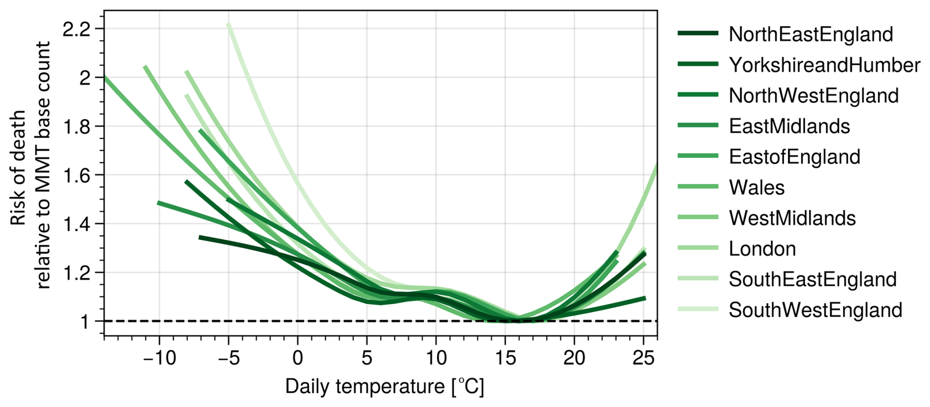
Figure 7 Exposure-response curves for mortality risk as function of temperature for different regions in the UK based on the DLNM approach. Regions are roughly sorted from North (dark colours) to South (light colours). The x-range of each curve is determined by the observed range of temperature values.

Throughout this study, mortality impacts are quantified as expected excess deaths derived from differences between stratospherically nudged and control ensemble simulations. These estimates therefore represent conditional, model-based expectations of mortality impacts given the presence of an SSW, rather than direct attribution of observed deaths.

4.2 Mortality impact of SSWs within the UK

To assess the impact of the February 2018 SSW on mortality in our numerical experiments (see Sect. 2.3) we use exposure–response curves (as derived in Sect. 3.1). This way we can simply take the surface temperature output of the model to compute an expected death count within each simulation.

Note that the exposure-response curves are estimated on ERA5 temperatures but evaluated on model output, so a residual mismatch between the two datasets remains. Because mortality impacts are inferred from differences between nudged and control simulations, systematic offsets in absolute model temperature largely cancel, although this cancellation is not exact given the non-linearity of the exposure-response curve. A formal bias correction (e.g. quantile mapping) would require a model climatology for each forecast system, which is not available for the SNAPSI re-forecasts. Figure 2 gives an indication of the variability across individual models and re-analysis. We further note that our analysis targets a single event rather than multi-event statistics, so a full bias correction would be of limited additional benefit here. The consistency of results across five independent forecast systems provides some reassurance that residual biases do not dominate our conclusions.

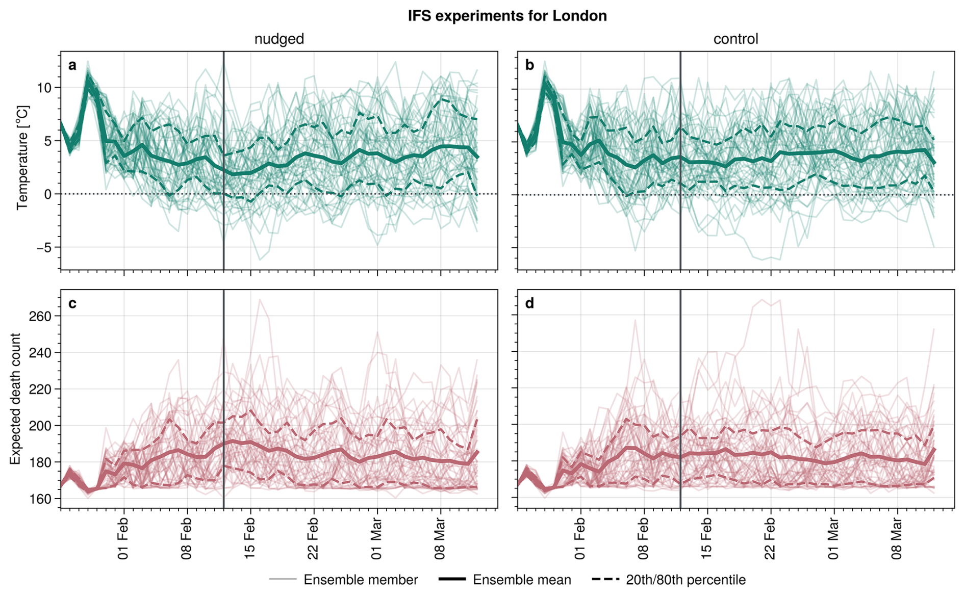
Figure 8 Example of an ensemble simulation for (a, b) temperature and (c, d) expected death count in London based on the IFS model. Shown are the nudged (a, c) and control (b, d) SNAPSI experiments. Death counts are computed from temperature using the DLNM exposure-response curve. Vertical solid lines indicate the SSW onset on 12 February.

Figure 8 illustrates an example of temperatures in London and the associated expected death counts for the nudged (with SSW) and control (without SSW) SNAPSI experiments obtained from the IFS model. Any differences between the nudged and control experiments in expected death counts can then be directly attributed to the occurrence of the SSW.

Throughout this section, reported mortality impacts refer to the attributable number of deaths as defined in Eq. (2), i.e. the difference in expected deaths between the nudged and control ensembles. Note that we can only compare statistical properties of the ensemble distribution (like the ensemble mean), and individual members cannot be compared.

Figure 9a shows a clear negative temperature anomaly in the multi-model mean (MMM) for London for essentially the entire covered period following the SSW (about 6 weeks). This anomaly reaches magnitudes of roughly 1K and can by construction be attributed to the SSW. Since the exposure-response curve for London steeply increases with decreasing temperatures (Fig. 3) this negative temperature anomaly is associated with a pronounced positive expected death rate anomaly which reaches about 4 deaths d⁻¹ in early March. This increase in death rate leads to an estimated total number of excess deaths attributable to the SSW for London of 91, when averaged over the entire period after the SSW.

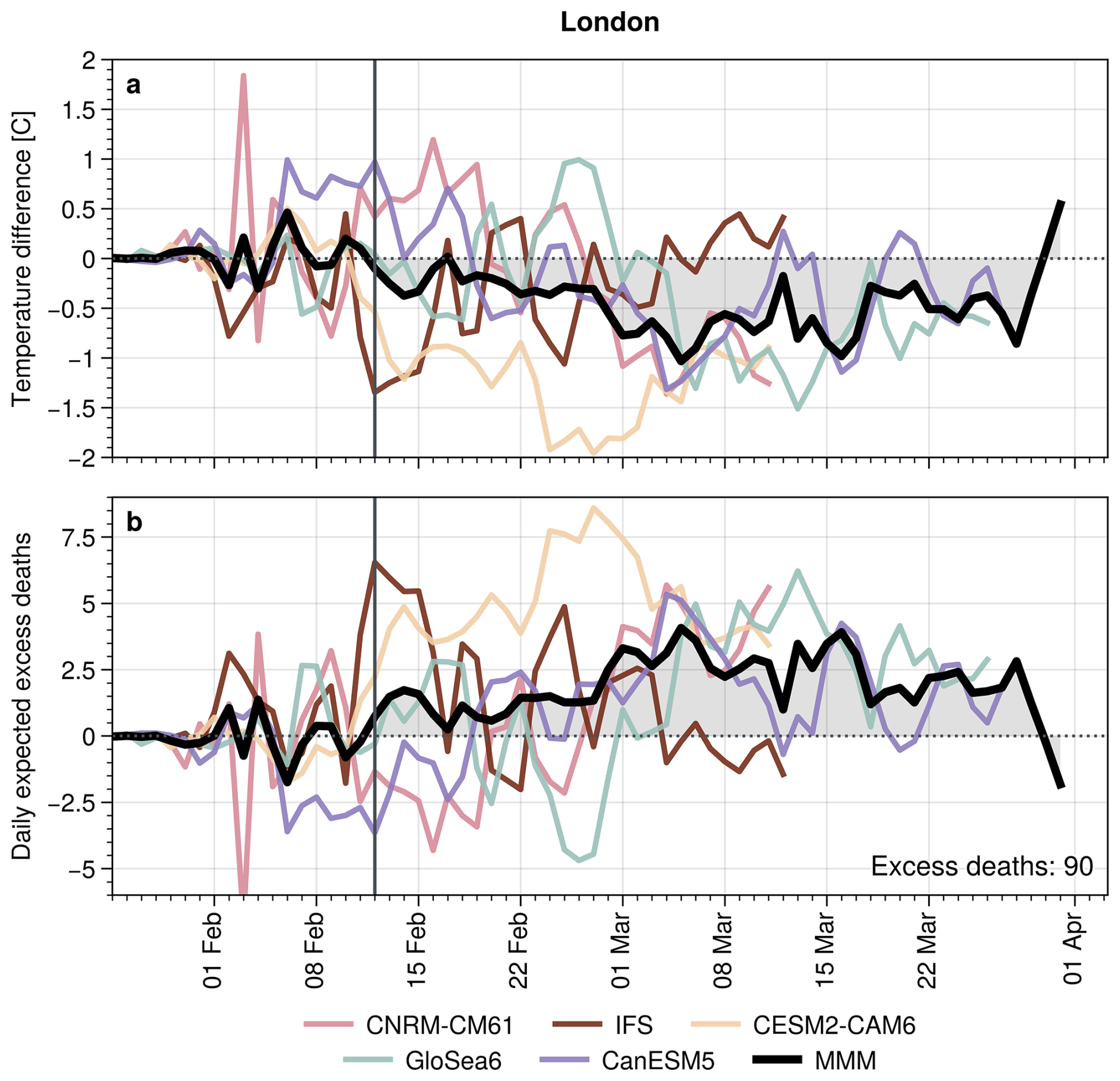
Figure 9 Difference in (a) temperature and (b) expected death count between nudged and control experiments for example of London and different models. Multi model mean is shown as thick black line with area between the curve and the x axis being highlighted. Death counts are computed based on the DLNM exposure-response curve. Vertical solid lines indicate the SSW onset on 12 February. Total excess deaths are computed as time average of the multi-model mean (MMM) from the SSW onset to 31 March. Note that different models have different integration lengths and hence contribute differently to the MMM.

An analogous analysis as shown in Fig. 9 can be performed for other UK regions and using the different approaches described above to derive the underlying exposure-response curves. Figure 10 compares the average increase in excess deaths and relative risk attributable to the SSW for different UK regions, as well as temporal resolution of input data and exposure-response models (DLNM vs. binning approach). Note that we only consider the first 30 d following the SSW onset in Fig. 10 to make different input temporal resolution easier to compare. The estimated death risk from the daily DLNM varies between about 0.7 % in South East England and 1.6 % in North West England. However, no clear north-south gradient is apparent.

Figure 10 Attributable SSW impacts on mortality for different UK regions. Shown are (a) the daily excess deaths and (b) the relative risk anomaly, both estimated as MMM difference between nudged and control experiments and averaged over the 30 d following the SSW onset. Risk anomaly is computed as difference between risk in nudged and control experiments. Different bars are based on different exposure-response models and underlying data with different temporal resolution. Total death rates for England+Wales are the sum of all regions, while the total risk anomaly is given as average over all regions.

Comparing the DLNM and binning approaches for daily input data shows a high degree of agreement, consistent with our findings from Fig. 4a. Estimates based on weekly data (using either the DLNM or the binning approach) remain close to the daily ones for most regions. Agreement is poorer for monthly inputs: while some regions still match the higher-resolution results closely (e.g. South West England or East Midlands), monthly inputs overestimate the attributable impact by up to a factor of about two in Yorkshire and Humber. Monthly-resolution estimates should therefore be read as indicating the sign and order of magnitude of the signal rather than as quantitative attribution. Figure S3 shows a subset of these combinations together with the spread between estimated mortality risk increases based on the different forecast systems, which is comparable to or larger than the differences between exposure-response models for most regions.

On average, our analysis estimates the excess deaths attributable to the February 2018 SSW to be around 15 deaths d⁻¹ throughout England and Wales for a period of 30 d, which is an increase of about 1 % compared to the average winter-time death count.

4.3 Different impacts of SSWs between UK and the Nordics

To contrast the mortality analysis for the UK, this section applies our framework to the Nordic countries of Norway, Finland and Sweden. Figures 2 and 1 show that the post-SSW temperature anomaly is typically much stronger in these Nordic countries, compared to the UK. However, the magnitude of any mortality impacts is a priori not clear due to the strong degree of non-linearity in some of the exposure-response curves. In fact, the Nordic countries tend to be associated with relatively flat exposure-response curves compared to the UK (see Fig. 11). The modelled daily mortality risk increases by about 20 % in Norway and about 40 % in Sweden and Finland for the most extreme cold anomalies recorded in our dataset relative to the risk at the MMT. However, note that some of these changes are potentially risk model-dependent. Figure 11a shows that in the case for Finland and weekly data, the DLNM approach produces a steeper curve than the binning approach. However, the DLNM approach does not systematically produce steeper tails, as e.g. shown in Fig. S2a for London. The risk increases of about 20 % to 40 % for Nordic cold extremes compare to risk increases ranging from 40 % to 120 % for individual regions in the UK (Fig. 7) based on daily data. Note that the exposure-response curves for UK are also steeper than the ones for the Nordics for purely monthly data (Fig. S4). Another significant difference between the UK and Nordic mortality curves is the MMT itself, with MMT in the UK being about 5 to 10 °C warmer compared to the Nordic countries. However, this shift in MMT alone does not seem to explain the resulting differences in attributable mortality without an additional change in steepness.

Figure 11 Exposure-response curves derived for (a, d) Finland (b, e) Sweden and (c, f) Norway based on input data with (a, b, c) weekly or (d, e, f) monthly mean temporal resolution. The solid and dashed lines in panel (a) are derived using a DLNM and binning approach, respectively, all other lines in other panels are derived using a binning approach. Red dots show death counts versus temperature distribution at the corresponding temporal resolution and location, divided by death counts at the MMT. Shading indicated the 95 % confidence interval around the curve. Note that daily data is available for Norway but not shown. Monthly means for Sweden and Finland are computed from weekly data as 4-week running mean. Weekly and monthly data for Norway is computed as direct average over fixed week-of-year or month-of-year bins.

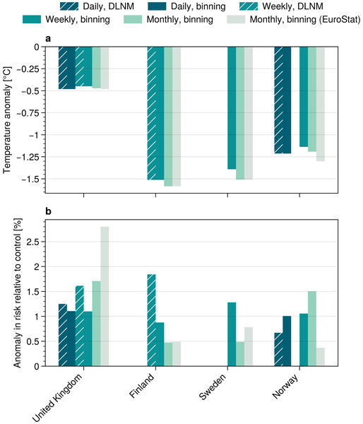
The differences in shape of the exposure-response curves then translate into non-trivial differences between estimated excess deaths for the different countries. Figure 12 compares the decrease in temperature and the associated increase in mortality risk following the SSW in the UK and different Nordic countries based on different mortality models and input temporal resolutions (note that certain UK datasets only assess the risk for England and Wales). Overall, the UK shows robustly weak mean temperature anomalies of about −0.5 °C compared to anomalies exceeding −1 °C throughout the Nordics and reaching up to −1.5 °C. However, the mortality risk increase in the UK is estimated to be at least as strong (if not stronger) than in the Nordics. While the UK shows an increased risk of 1 % or more despite its weaker temperature anomaly, estimates for the Nordic countries are of comparable magnitude and vary more strongly between approaches. Although estimates vary between impact model types and input datasets, all regions show positive risk anomalies due to the negative temperature signals associated with the SSW. Figure S5 repeats this comparison for a subset of model and resolution combinations with uncertainty bars indicating the spread between forecast systems. This spread is substantial and, for most countries, comparable to or larger than the differences between exposure-response models, so the ordering between individual countries should not be over-interpreted. (Note the large spread in risk anomaly for Sweden in Fig. S5, which is likely a direct result of the strongly limited coverage in our dataset – see Table 2.)

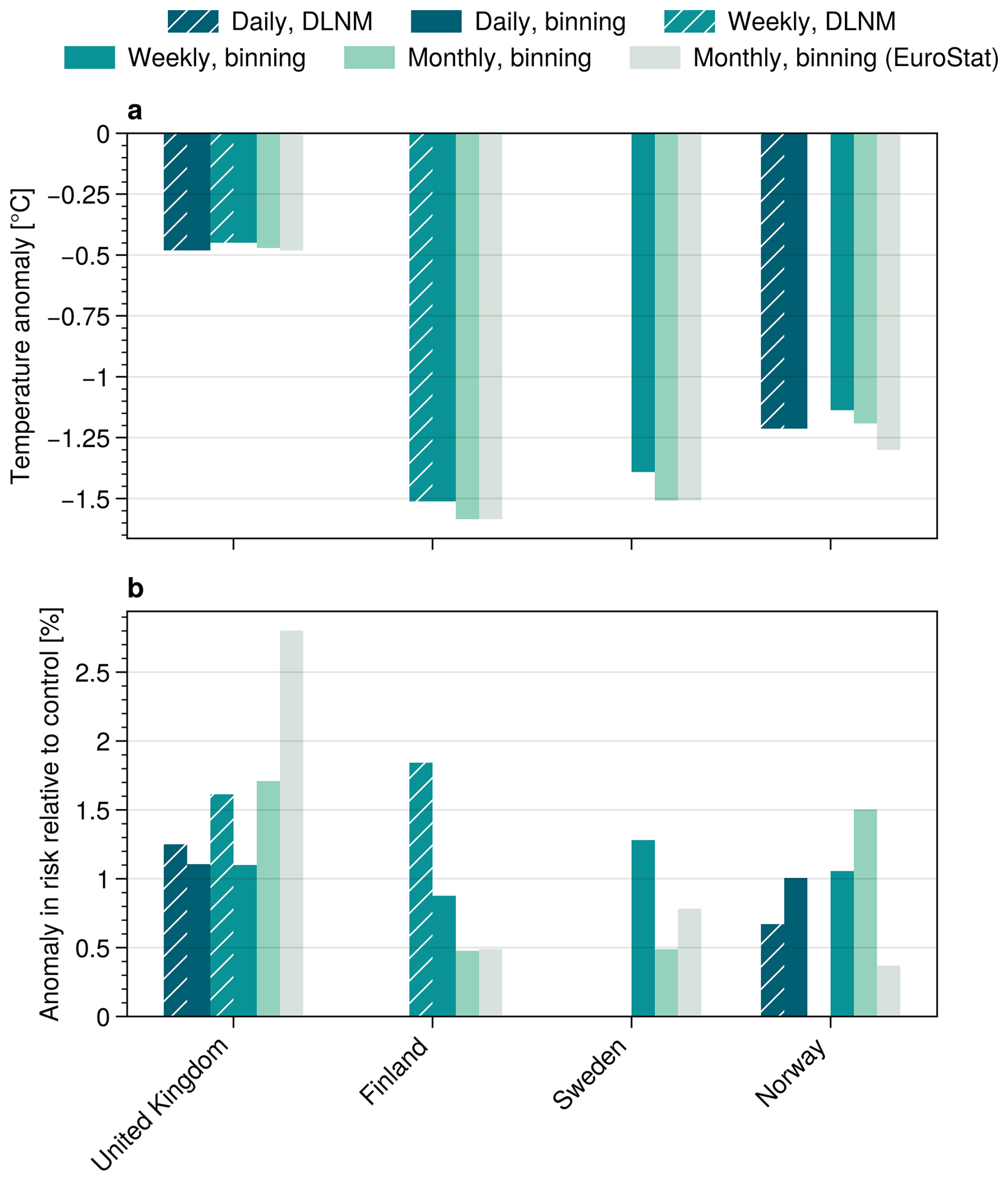
Figure 12 Meteorological and socio-economic impacts in the 30 d following the SSW. (a) Temperature anomaly and (b) mortality risk anomaly for different countries. All data is given as difference of nudged and control experiments with mortality computed via exposure-response curves based input data with different temporal resolutions and different model approaches (DLNM or binning). Anomalies are computed from daily, weekly or monthly data, based on availability. Note that the EUROSTATS dataset includes data for the entire United Kingdom, while all other UK datasets only contain England+Wales. Further recall that the different datasets cover different time period.

The effect of the SSW on absolute death counts are quantified in Table 4, showing best-estimates based on the highest available temporal resolution data and the DLNM approach where data of sufficient quality was available. The estimates are based on the full period following the SSW with avavailable model data, i.e., 12 February to 31 March (in contrast to some earlier results based on 30 d post-SSW).

Table 4 Estimated deaths and changes in mortality risk attributable to the 2018 SSW in different regions for specific model and dataset combinations. The attributable risk increase is the difference in relative mortality risk between the nudged and control ensembles, expressed in percent. Uncertainty ranges show 10th and 90th percentile of bootstrapped MMMs for all possible 5-model combinations (see Sect. 2.3).

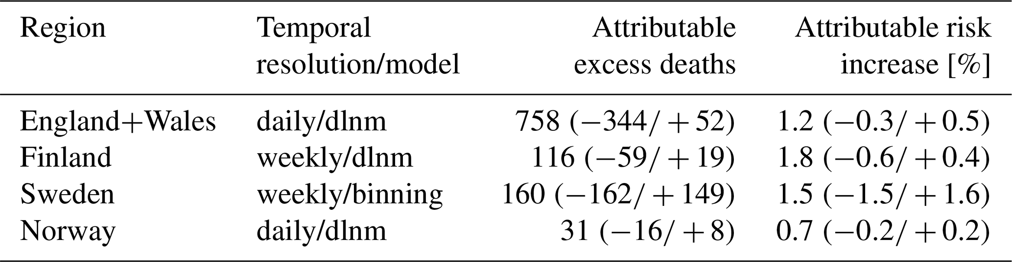
We find that the February 2018 SSW is associated with an expected excess of about 750 deaths in England and Wales, based on differences between stratospherically nudged and control ensemble simulations and a combined count of about 300 expected deaths in the Nordic countries Finland, Sweden and Norway. The ranges quoted in Table 4 reflect the spread between forecast systems alone and are correspondingly wide; they do not include the structural uncertainty associated with the choice of exposure-response model or associated with the choice of parameters within a model, some of which are illustrated by the different bars in Figs. 10 and 12.

5 Discussion and conclusions

This study presents a counterfactual attribution framework to assess health impacts of meteorological phenomena, applying it specifically to the February 2018 SSW event and its associated cold surface anomalies. By combining exposure–response curves with stratospherically nudged ensemble forecasts, we demonstrate a robust method to quantify mortality impacts attributable to stratospheric variability by explicitly comparing an SSW-exposed and an SSW-unexposed model world. Our ensemble-based attribution framework indicates an expected excess of several hundred deaths in England and Wales (best estimate about 750, with a range of roughly 400 to 800 across forecast systems) and a few hundred combined total deaths in the Nordic countries (best estimate about 300, ranging from roughly 100 to 500) linked to the post-SSW temperature anomalies of 2018 (Table 4). Here, our estimate might pose a lower bound on the actual number of attributable deaths, as we are restricted by the finite length of the numerical ensemble simulations. Figure 9 suggests that temperature and mortality signals could still be present after 31 March. The actual number of expected deaths attributable to the strong SSW event in early 2018 might be even higher. However, note that our attributed mortality impact for the UK is generally consistent with the mean SSW mortality impact of 620 deaths found by Charlton-Perez et al. (2021).

Our analysis underlines that the relationship between temperature anomalies and mortality risk is non-trivial and often highly non-linear (e.g., Gasparrini et al., 2015), and further shows that these characteristics also apply to cold anomalies associated with stratospheric variability. Although the Nordic countries experienced the strongest post-SSW temperature drops, the attributable increase in mortality risk in the UK was overall higher (Fig. 12). This can be understood through the highly non-linear shape of the exposure-response relationship, with extremely steep cold branches in regions less adapted to cold conditions. For instance, we find a clear north-south gradient within the UK, where southern regions such as London and South West England show a sharper increase in mortality risk at lower temperatures than their northern counterparts (Fig. 7). A similar pattern is observed at the city level in Norway, with Bergen exhibiting an unusually steep cold-branch response compared to the other cities studied (Fig. S6), potentially due to its typically mild, ocean-moderated winter climate. Nevertheless, we do not find such a clear overall north-south gradient in Norway.

Interestingly, while the exposure-response curves for southern UK regions tend to be steeper, the resulting risk anomalies are not systematically larger than those in the north (Fig. 10). One reason might be that the increased steepness of the exposure-response cold branch towards the south compensates for the generally smaller post-SSW temperature anomalies observed in these regions (Fig. 2). This balance further highlights the need to consider both hazard magnitude and population vulnerability when assessing health impacts. Beyond climatological adaptation, demographic or socioeconomic factors may also play a role in shaping regional differences. Such factors could comprise of baseline health conditions, urban heat retention, or heating practices, although the precise role of additional influences remains beyond the scope of the current dataset and merits further targeted investigation.

Methodologically, we show that the presented framework is flexible and yields consistent results across different modeling approaches and data resolutions (e.g. Fig. 10). The epidemiological component of this framework is standard: exposure-response relationships are estimated with an unmodified DLNM and the attributable number of deaths follows from the usual definition (Eqs. 1 and 2). Evaluating such exposure–response functions on temperature series from model simulations rather than from an observed record is likewise established practice in health impact projections (e.g., Gasparrini et al., 2017; Vicedo-Cabrera et al., 2021). The novel element here is the meteorological one: the reference state is provided by an SSW-free control ensemble, which isolates the contribution of a single stratospheric event. While DLNMs offer a theoretically grounded estimate of the lagged mortality response, our simpler binning-based method also proves effective to estimate orders of magnitude, even when applied to coarser temporal inputs such as monthly mortality data.

A key distinction from many temperature-mortality studies focused on short-lived cold spells is that SSW-related circulation anomalies persist on subseasonal timescales of several weeks to months. This persistence makes it plausible that aggregated mortality products retain a usable signal in this specific attribution setting and our weekly-resolution results are indeed close to the daily ones. We are more cautious about monthly records, where deviations from the daily estimates are larger in individual regions. Where only aggregated health data are available, the methods of Basagaña and Ballester (2024) offer a principled alternative to the simple aggregation used here. Higher temporal resolution mortality data nonetheless remains clearly preferable where it can be obtained.

In a similar way, the large-scale nature of the SSW response (cf. Fig. 1) allows for relatively coarse temperature metrics (e.g. country-level means or representative points). While population-weighted temperature series could, in principle, refine absolute exposure estimates (particularly in regions with uneven population distributions) the spatial coherence of SSW-induced anomalies and our difference-based attribution framework likely mean that this simplification does not materially affect the inferred relative, event-based impacts. We can test this directly for England and Wales, where region-specific temperature series are available. Repeating the regional DLNM fits using a single common temperature series taken from the centre of England and Wales, rather than each region's own series, has only limited effect on the pooled exposure-response curve (Fig. S7). This supports the use of a single representative series where regionally resolved exposure is not available, as is the case for the Nordic countries. The weak sensitivity to the temperature proxy in Fig. S7 also illustrates a more general property of our framework: because the exposure-response curves are constructed from the same temperature series that is later used for the attribution, a systematic offset between the chosen series and the true population exposure is absorbed into the fitted curve and does not propagate into the difference between the nudged and control worlds. What is not absorbed is the residual scatter between the two, which would attenuate the fitted curve, and it is this component that the comparison above is designed to test.

For the same reason, we estimate exposure-response curves from our own mortality and re-analysis records rather than adopting published city-level functions (e.g., Masselot and Gasparrini, 2023). Using an external curve requires the exposure variable to be defined consistently between the fit and the evaluation, which is not guaranteed across different spatial definitions and processing chains, and the benefit of a finer-resolution curve is in any case limited by the resolution of the nudged ensemble output. Such functions would nonetheless be a natural starting point for extending the framework to a larger set of European locations, particularly in combination with higher-resolution meteorological input.

We note, however, that uncertainties in the construction of exposure-response curves remain large. These include sensitivity to choice of statistical model, temporal aggregation and lag assumptions, particularly for extreme temperatures where sample sizes are small. This is especially relevant in smaller regions such as individual Norwegian cities (Fig. S8), where daily death counts often remain in the single digits and introduce considerable statistical noise. A further contribution arises from the estimate of the baseline death count n_MMT itself (Sect. 3.1), which differs by on the order of 10 %–20 % between the climatological and observation-based routes depending on the region. Together with the spread between forecast systems, this means that the absolute numbers reported here should be read as rough estimates rather than as precise counts.

Our attribution analysis specifically studies the February 2018 SSW event, chosen due to its pronounced temperature anomalies and clear societal impacts. However, attributing impacts across the broader distribution of SSW events requires careful consideration. While composite mean temperature anomalies averaged over multiple SSWs (cf. Fig. 2) can provide a general indication of expected impacts, they might underestimate the actual societal consequences. Mortality and other health impacts tend to be disproportionately influenced by extreme temperature anomalies rather than mean conditions. Particularly severe SSW events (like in early 2018) likely dominate the statistics on cumulative mortality impacts. Robust attribution of these disproportionate impacts require ensemble approaches similar to the one employed here (i.e. SNAPSI experiments), as such methods effectively isolate and quantify the contribution of individual, high-impact SSW events.

While this study focuses primarily on mortality impacts, SSW-triggered cold spells also carry substantial consequences for broader societal sectors, including transportation, energy demand, agriculture, and economic productivity (e.g., Büeler et al., 2020). Extending the presented analytical approaches to these sectors could enhance preparedness and adaptation strategies, especially where risk relationships are similarly non-linear. In particular, our findings on regional variation in exposure-response steepness may offer valuable insights for climate adaptation planning.

Future research could also apply the framework more broadly across Europe to assess SSW-related mortality in additional regions (analogous to, e.g., Analitis et al., 2008). Where only aggregated health records are available, methods that recover daily-scale effects from weekly or monthly counts (Basagaña and Ballester, 2024) would be the appropriate route. Furthermore, complementing all-cause mortality with metrics such as years of life lost (YLL) or cause-specific impacts (e.g. respiratory illness) may help better capture the socio-demographic variation in vulnerability (e.g., Arbuthnott et al., 2020). In addition, methodologies such as the fractional attributable risk (FAR) approach could allow to extract attribution signals from re-forecast datasets without the need for nudging or other manipulation of the numerical model. Spaeth and Birner (2022), for example, used the FAR approach to statistically attribute Arctic Oscillation extremes to stratospheric events. Combining different approaches (like nudged experiments and FAR) could further enhance the scalability and applicability of our attribution framework.

Two important considerations apply to our use of stratospherically nudged ensemble forecasts. First, while this approach effectively isolates the downward influence of SSWs, the stratosphere-troposphere coupling is inherently bidirectional. Nudging the zonal-mean wind suppresses some of the upward feedback from the troposphere, which may lead to slightly unphysical evolutions near the SSW onset (Hitchcock et al., 2022). Second, the results are likely sensitive to the forecast initialisation date. Runs initialised too close to the SSW may not allow sufficient time for stratospheric signals to influence the troposphere. Our choice of 25 January offers a compromise, ensuring that both the nudged and control scenarios represent plausible futures in which downward propagation of the stratospheric signal could occur.

Overall, we think that our analysis framework represents a promising tool for the attribution of weather-related societal impacts. While applied here to cold spells triggered by a specific SSW event, the approach is generalizable to other meteorological drivers such as heatwaves, precipitation extremes, or air pollution events. The methodological approach offers a flexible basis for analysing impacts across diverse spatial and temporal contexts, helping to bridge atmospheric variability with real-world societal risks in a policy-relevant way.