Composition, frequency, and severity of future rain-on-snow floods in Germany

In Germany, severe widespread winter floods are often generated by rain-on-snow (ROS) phenomena. Under suitable conditions, when rain falls on the snow cover, the snow can melt and produce extreme amounts of runoff. In a warming climate, the frequency of ROS events is expected to change locally depending on elevation and regionally based on the general climate conditions. Consequently, the characteristics of ROS-driven winter floods are also anticipated to change. To investigate these changes, streamflow for multiple gauge stations in Germany was simulated using an ensemble of Long Short-Term Memory models based on an ensemble of downscaled climate projections. Germany, as a representative mid-latitude country with a considerable portion of historical floods generated by ROS, offers extensive spatial and temporal coverage of hydrological observations spanning long temporal scales, and hence warranting efficient training of the deep learning model. We used an explainable artificial intelligence method, integrated gradients, to examine flood-generating processes, focusing primarily on ROS, for every simulated flood peak. Changes in frequency, feature importance, and a ranking based severity of ROS flood events were assessed for individual streamflow gauges and for widespread floods affecting multiple catchments across four major river basins in Germany. We found that with regard to the ensemble median, the frequency of ROS floods will mostly decrease at the scale of individual gauges by up to 60 %, as well as at the widespread scale for the Rhine, Elbe, and Weser River basins but increase at gauges located in the Danube River basin for the corresponding widespread floods. For all regions, the snowmelt component during ROS floods becomes less relevant, whereas the contribution of rainfall to these events increases. Interestingly, the severity of the mean and the most extreme widespread ROS floods is projected to increase compared to the historical period in all major river basins in Germany. Only for individual gauges the severity may decrease in the future. Despite the overall agreement in the trends of the input features across climate models, the resulting trends in ROS floods are considerably disparate. This discrepancy is primarily attributed to complex model chains in the climate models leading to variability in rainfall and snowmelt, and to different melting seasons.

1 Introduction

Events in which rain falls on an existing snowpack and generates additional runoff are called rain-on-snow (ROS) events. Such events are very common in mid-latitude regions of the Northern Hemisphere (Cohen et al., 2015) such as the Pacific Northwest USA and Canada (e.g., McCabe et al., 2007; Trubilowicz and Moore, 2017), central and northern Europe, and Eurasia (e.g., Sui and Koehler, 2001; Ye et al., 2008; Pall et al., 2019), and high-mountain regions in Asia (e.g., Ohba and Kawase, 2020; Maina and Kumar, 2023). ROS events can produce large amounts of runoff, making them an important process for flood generation (Sui and Koehler, 2001; Merz and Blöschl, 2003). Both rainfall and snowmelt can contribute significantly to the generated runoff, with the dominant role varying depending on the location and season (Trubilowicz and Moore, 2017; Li et al., 2019). During ROS events, rainfall plays a critical role by saturating the snow cover and triggering fast runoff (Rössler et al., 2014).

ROS events occur primarily from October to May in low- to mid-elevation regions (McCabe et al., 2007; Cohen et al., 2015), but have also been reported in September and during the summer months, especially in high-elevation regions (McCabe et al., 2007; Morán-Tejeda et al., 2016; Beniston and Stoffel, 2016). With increasing temperatures fueled by global warming, changes in the frequency and magnitude of runoff generated by ROS events, as well as a higher associated flood risk, are expected (Freudiger et al., 2014; Musselman et al., 2018; Chegwidden S et al., 2020). Observations generally indicate an increase in ROS frequency for high-elevation basins, while lower-elevation regions show a decrease, depending on the season (Freudiger et al., 2014; Pall et al., 2019; Ondrej Hotovy and Jenicek, 2023). These studies attribute the change in ROS frequency mainly to an increased frequency of rainfall during the winter half of the year, which is the result of warmer air temperatures, and to the lack of persistence of a pre-existing snowpack.

Many studies have investigated changes in the frequency, timing and magnitude of floods using observations and climate projections. Depending on the region, flood type and severity, these studies have indicated both increasing and decreasing trends (e.g., Petrow et al., 2009; Rojas et al., 2012; Blöschl et al., 2019; Bertola et al., 2020; Huang et al., 2022; Chegwidden S et al., 2020; Tarasova et al., 2023). Blöschl et al. (2017) demonstrate a spatially heterogeneous trend in flood timings across Europe, finding that floods related to snowmelt tend to occur earlier in the year. Similar to the changes in flood timings, changes in flood magnitude are also spatially heterogeneous across Europe, although clear patterns emerge for regions experiencing an increase or a decrease in flood magnitude (Blöschl et al., 2019).

For the USA, Huang et al. (2022) observe a decrease in the frequency and magnitude of ROS-driven floods during the period from 1960 to 2018. This trend of decreasing ROS-driven floods is projected to continue in an RCP8.5 scenario (Chegwidden S et al., 2020). For an RCP4.5 scenario the decrease in ROS-driven floods is similar in low-elevated basins, but much weaker in mid to high-elevated basins. In contrast, using a lumped conceptual hydrological model to simulate streamflow for a future RCP4.5 scenario in Europe, Sezen et al. (2020) find that for two rivers located in small catchments (60–160 km²) in Slovenia, the frequency of ROS floods may increase, with a peak in the period from 2041 to 2070 along with a generally weaker seasonality. Their results also suggest that the median ROS flood magnitude will decrease, while extremes could become stronger. Also, Beniston and Stoffel (2016) find that for a basin located in Switzerland, a temperature rise of 4–5 °C will increase ROS frequency by about 40 % at low elevations and 200 % at high elevations. With this amount of temperature increase, there is still enough snowpack left to trigger ROS events and an increased frequency of rainfall. However, for temperature increases of more than 5 °C the decrease of the snowpack is too large and this trend reverses.

Germany, as an example of a mid-latitude country in Central Europe, has many rivers of varying elevation that are frequently affected by ROS events (Sui and Koehler, 2001; Freudiger et al., 2014; Tarasova et al., 2020a). The current understanding of changes in ROS events in Germany is fragmented. On one hand, the simulations of ROS events by Dong and Menzel (2020) show a significant reduction of the snow water equivalent (SWE) during winter periods during 1961 to 2016 in Rhineland-Palatinate, a mid-range upland region located within the Rhine basin in Germany. On the other hand, their simulations show that the ROS frequency increases in February since the 1990s, while there has been a decrease in January and March. For the major basins in Germany, Freudiger et al. (2014) found an increase in ROS magnitude in upland basins, during the latter half of the period from 1950 to 2011, but at the same time a decrease in ROS frequency in both upland and lowland basins.

Kemter et al. (2020) investigated the relevance of flood-driving mechanisms and their change at individual gauge stations in Europe for a downscaled reanalysis data set during the time period from 1960 to 2010. They find that soil moisture excess has the largest relevance in northern and middle Germany followed by ROS, snowmelt and stratiform rain. Floods generated by ROS account for 20 %–30 % of all floods. Similarly, Tarasova et al. (2023) also find that 20 %–30 % of mean annual floods in Germany are generated by ROS, while most floods are generated by rain on wet soils. Kemter et al. (2020) find a negative shift in relevance for snowmelt in middle to southern Germany and a positive shift in ROS in these areas. Outside these areas, ROS becomes less relevant. These findings are supported by the findings of Tarasova et al. (2023), who also find a decrease in ROS flood frequency in the time period from 1960 to 2010.

Severe river floods in Germany are often widespread and affect a large part of the river network across multiple catchments, with 40 % of all floods affecting more than 30 % of the river network (Uhlemann et al., 2010), and therefore can have high socio-economic impacts and loss of life (Ulbrich and Fink, 1995; Ulbrich et al., 2003; Petrow et al., 2006; Merz et al., 2014, e.g.,). Most of these widespread floods, and especially the most severe floods, occur in winter with an increasing frequency in recent decades (Uhlemann et al., 2010). A large number of the most intense widespread floods are associated with ROS events (Krug et al., 2020), which highlights the great relevance of ROS floods on a multi-catchment scale compared to individual gauges.

Recent studies about changes flood properties in Europe either use observational data, do not distinguish between flood types, focus on a single or very few catchments or use a small number of climate projections when they investigate changes under future climate scenarios. The results of Sezen et al. (2020) show a great variability in terms of projected changes in ROS flood frequency and severity between the different climate models. Two different models could project divergent trends in frequency and severity of ROS floods for the same emission scenario.

This underlines the need of an ensemble-based assessment of trends in flood-generating processes. Therefore, we use a computationally cheap deep learning approach, an ensemble of Long Short-Term Memory models (LSTM) (Kratzert et al., 2018), which allows us to simulate streamflow for a large ensemble of climate simulations under the high-emission RCP8.5 scenario at multiple gauge stations in Germany covering a variety of catchment sizes and elevations. Additionally to changes at localized individual gauge stations, we provide an insight into changes to flood events on widespread, multi-catchment scale.

Because we specifically want to focus on ROS floods, we need to attribute flood generating processes to single flood events. However, this attribution strongly depends on the method and perspective of the classification (Tarasova et al., 2019). Tarasova et al. (2020b) show that a significant part of classification uncertainty originates from the uncertainty of the hydrological model.

Recent studies show that deep learning models perform as well or even better than regular hydrological models (Nearing et al., 2024; Frame et al., 2022) even when high flow events are not included in the training data. To overcome the issue of classification uncertainty and to isolate the variability of climate models, we use our simulations in combination with an explainable artificial intelligence (XAI) technique, integrated gradients, to interpret the feature importance each simulated flood peak. We then apply a ratio-based classification of the feature importance as suggested by Tarasova et al. (2020b) to identify ROS-generated floods.

2 Data and Methods

2.1 Study area and training data

We consider 97 streamflow gauges (Fig. 1) located in the German parts of the Rhine, Danube, Elbe, and Weser River basins. The gauges were selected based on the availability of daily river discharge and corresponding watershed boundaries from the Global Runoff Data Centre (GRDC) data set (https://grdc.bafg.de/, last access: 28 October 2026), as well as based on the availability of classification of flood peaks based on their generation processes from the previous study of Tarasova et al. (2020b). The time series of 72 gauge stations begin in 1950, 13 in the 1950s, 9 the 1960s, and 3 in the 1970s. The sizes of the study catchment areas range from 127 to 23 719 km².

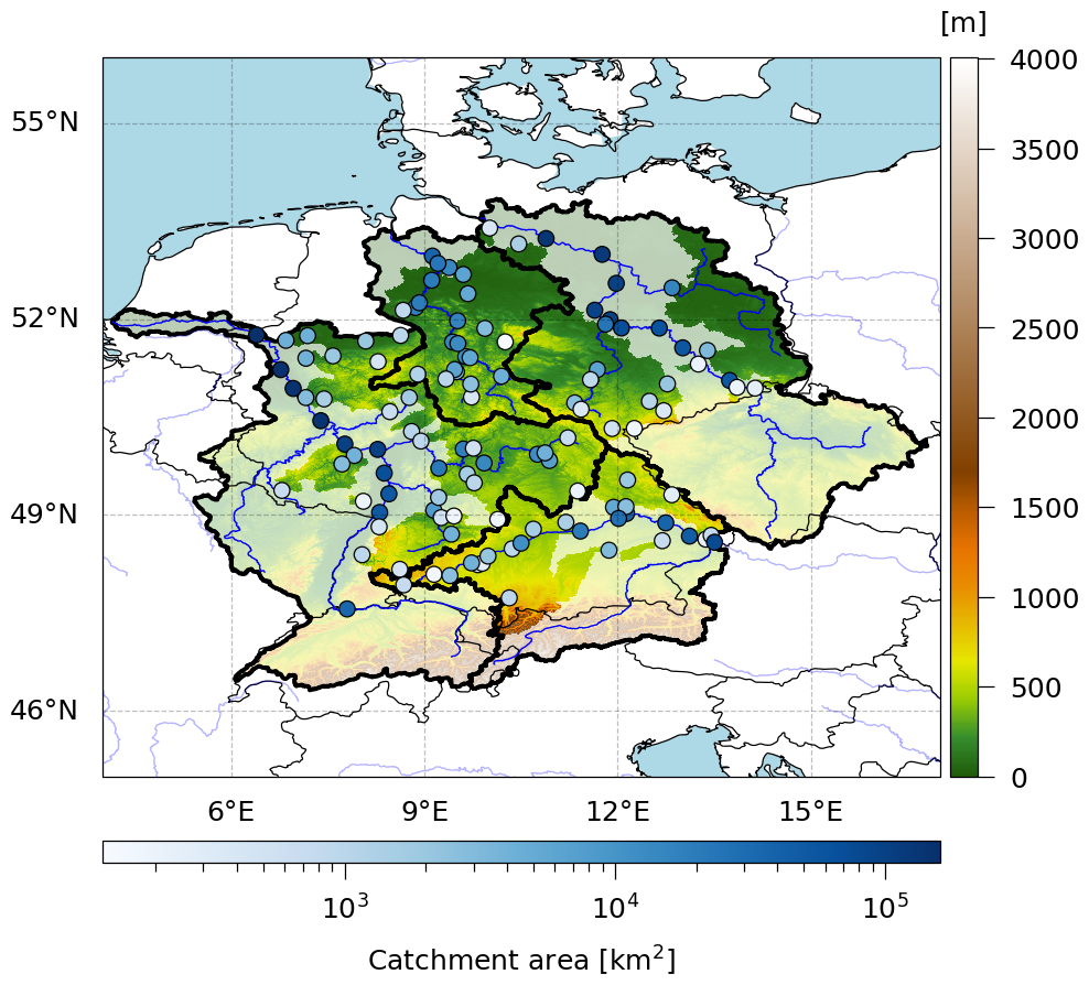
Figure 1 Study area and gauge stations. The thick black outlines show the Germany affecting parts of the 4 major river basins of the Rhine, Danube, Elbe and Weser rivers. The gauge stations are represented by the circles, with the blue color scale representing their basin area. The non-transparent parts of the major river basins are covered by the gauge stations. The elevation data is taken from the ETOPO Global Relief Model (NOAA National Centers for Environmental Information, 2022).

The deep learning model was trained using the ERA5 reanalysis data set (Hersbach et al., 2020) to simulate observed streamflow. The ERA5 data has a spatial resolution of 0.25° × 0.25° and were aggregated or averaged to a daily temporal resolution. The input features for the LSTM included catchment-averaged near surface temperature, liquid precipitation, snowfall, snowmelt, snow amount, surface runoff, subsurface runoff, and day length. Liquid precipitation was calculated by subtracting snowfall from total precipitation. Surface and subsurface runoff were used as a proxy for soil moisture. In the atmospheric data sets, water from precipitation or snowmelt that is not stored in the soil is considered runoff. For ERA5, surface and subsurface runoff are available as separate variables. For climate projections (see Sect. 2.5) the subsurface runoff was calculated by subtracting surface runoff from total runoff.

Day length was calculated using an adapted formula following Forsythe et al. (1995)

$$\begin{array}{}\text{(1)}& {\displaystyle }\mathrm{daylength}={\displaystyle \frac{\mathrm{2}}{\mathrm{15}}}\arccos (-\tan (\mathit{\varphi })\cdot \tan (\mathit{\delta }\left)\right)\text{(2)}& {\displaystyle }\mathit{\delta }=-\mathrm{23.45}\cdot \cos \left({\displaystyle \frac{\mathrm{360}}{\mathrm{365}}}\cdot (d+\mathrm{10})\right)\end{array}$$

where ϕ is the latitude of the gauge station and d is the day of the year.

2.2 Deep learning model

Streamflow was simulated using a Long Short-Term Memory (LSTM) model (Hochreiter and Schmidhuber, 1997) with the base setup as described in Jiang et al. (2022a) and Jiang et al. (2022b). The model consists of a single LSTM layer with 32 neurons and a dense layer with 1 neuron. An adaptive learning rate, the adaptive moment estimation (Adam) optimizer (Kingma and Ba, 2017), and a batch size of 1024 were selected for model training. The past 150 time steps (in this case, 150 d) were used to simulate river discharge for each day in the time series.

For each individual gauge, we trained an ensemble of 10 independent LSTM models using different segments of the time series by applying 10-fold cross-validation to address the uncertainty of the streamflow simulation induced by the random initialization of model weights and by the training data (see Fig. S1 in the Supplement). We found that the impact of the training period on model performance is much larger than the effect of initial randomness and therefore prefer the cross-validation ensemble over an ensemble with only random initialization. The performance of the LSTMs on the test segments was measured using the Nash-Sutcliffe Efficiency (NSE) (Nash and Sutcliffe, 1970) and the Kling-Gupta Efficiency (KGE) (Gupta et al., 2009). For the final streamflow predictions the ensemble mean was taken by simply averaging the 10 folds of the ensembles.

As Kratzert et al. (2018) demonstrate, a regionally-trained LSTM outperforms an LSTM trained for individual catchments. However, Jiang et al. (2022a) point out that a regionally trained LSTM can complicate the interpretability of flood-generating processes. For this reason, in this study we opt for individually trained LSTMs.

2.3 Identification of flood-generating processes

For the identification of flood peaks, a simple peak over threshold (POT) method was applied to all discharge time series. The threshold was set to detect an average of 5 peaks per year. To ensure the independence of the peaks detected by POT5, we applied the criteria suggested by Lang et al. (1999), which states that two flood peaks must be separated by a time interval theta or have the intermediate flow drop below 75 % of the minimum of both peaks.

$$\begin{array}{}\text{(3)}& \mathrm{\Theta }>\mathrm{4.0483}+\log \left(A\right)\mathrm{or}{Q}_{min}<\mathrm{75}\mathit{\%}[Q_{\mathrm{1}},Q_{\mathrm{2}}]\end{array}$$

where A is the catchment area in square kilometres. Peaks detected using the POT method are referred to as POT5 peaks. Every peak exceeding the discharge of the flood with a return period of 2 years (Q₂) is considered a flood event.

Similarly to Jiang et al. (2022a), the flood-generating processes of the discharge peaks were analyzed using the XAI method integrated gradients (IG) (Sundararajan et al., 2017). This method interprets the model gradients used for predictions, providing the importance of each feature for each time step in predicting a single time step of the target variable. In this case, at a given time step (e.g., the date corresponding to a flood peak), the IG method computes 150 values (corresponding to the number of time steps used for prediction) for each input feature (i.e., 7 atmospheric variables and day length).

Since our focus is particularly on ROS floods, we only utilized liquid precipitation, snow amount, and snowmelt (i.e., input features that directly relate to the generation of ROS events) for the XAI analysis. However, it is important to note that all other input variables are crucial for the reliable performance of LSTM (i.e., removing any of them results in inferior model performance). All IG values were normalized to account for the different scales of the input features and to enhance comparability between the different peak magnitudes and gauges. Finally, a discharge peak was defined as ROS-driven if the proportion between the sum of absolute IG values of snowmelt (IG_sm) and snow amount (IG_snw), and liquid precipitation (IG_prl) was between 0.1 (very low importance of snowmelt and very high importance of liquid precipitation for flood generation) and 10 (very high importance of snowmelt and very low importance of liquid precipitation for flood generation) to exclude flood events mainly driven by rainfall or snowmelt:

$$\begin{array}{}\text{(4)}& {\displaystyle }{\mathrm{IG}}_{\mathrm{ROS}}={\displaystyle \frac{{\sum }_{n=\mathrm{0}}^{\mathrm{4}}\left|{\mathrm{IG}}_{\mathrm{sm}}\right|+\left|{\mathrm{IG}}_{\mathrm{snw}}\right|}{{\sum }_{n=\mathrm{0}}^{\mathrm{4}}\left|{\mathrm{IG}}_{\mathrm{prl}}\right|}}\text{(5)}& {\displaystyle }\mathrm{0.1}<{\mathrm{IG}}_{\mathrm{ROS}}<\mathrm{10}\end{array}$$

An IG_ROS value of 1 indicates equal importance for both features to the LSTM. We further investigate the suitability of the selected thresholds (see Result Section).

Generally, the values of IG_prl and IG_sm were positive (indicating that high liquid precipitation and snowmelt were important), while the values of IG_snw were negative (indicating that a snow amount lead to a reduction of the flood peak). Because most variables are not independent from each other, in some cases, the LSTM only considered snow amount important but not snowmelt, although a snowmelt peak was present in the data. Consequently, snow amount was included in the calculations, and the the absolutes of the IG values were used. To calculate IG_ROS for a given time step, the IG values were selected from a window of 5 time steps (the current and the past four time steps). This window was selected based on the linear correlation between the resulting IG_ROS values for the ERA5-driven simulated discharge peaks and the actual ratio of the snowmelt and liquid precipitation variables from ERA5 (see Fig. A1) and its suitability was further tested (see Results Section).

The XAI-based classification of flood events is evaluated using classified events from Tarasova et al. (2020b) as a benchmark. They used high-resolution (1 km) observational precipitation and snowmelt simulated by a regionally calibrated hydrological model (4 km). According to their definition, for a ROS event, both the ratio between total event snowmelt and the sum of total event snowmelt and rainfall (to exclude snowmelt floods) and the ratio between total event rainfall and the sum of total event snowmelt and rainfall (to exclude rainfall events) must be lower than 0.95. Additionally, they distinguished between ROS and spatially unrelated rainfall and snowmelt. As we do not have information on the spatial distribution of rainfall and snowmelt due to the catchment-averaging, both cases will be treated as ROS. As a measure of classification quality, multiple skill scores will be considered.

Accuracy is defined as the ratio of correct classifications to total classifications:

$$\begin{array}{}\text{(6)}& \mathrm{ACC}={\displaystyle \frac{\mathrm{TP}+\mathrm{TN}}{\mathrm{TP}+\mathrm{TN}+\mathrm{FP}+\mathrm{FN}}}\end{array}$$

Correct classifications are called true positives (TP) and true negatives (TN). False classifications are named false positives (FP) and false negatives (FN).

Precision is defined as the ratio of true positives and all detected positives (the sum of true positives and false positives):

$$\begin{array}{}\text{(7)}& \mathrm{PRE}={\displaystyle \frac{\mathrm{TP}}{\mathrm{TP}+\mathrm{FP}}}\end{array}$$

Recall is defined as the ratio of true positives and all actual positives (the sum of true positives and false negatives):

$$\begin{array}{}\text{(8)}& \mathrm{REC}={\displaystyle \frac{\mathrm{TP}}{\mathrm{TP}+\mathrm{FN}}}\end{array}$$

As we aim for the best possible match under consideration, that the frequency of ROS and non-ROS is not equal, the F1 score is used to balance false positives and false negatives. The F1 score is the harmonic mean of precision and recall and defined as:

$$\begin{array}{}\text{(9)}& F\mathrm{1}={\displaystyle \frac{\mathrm{2}\mathrm{TP}}{\mathrm{2}\mathrm{TP}+\mathrm{FP}+\mathrm{FN}}}\end{array}$$

For all scores, a value of 1 indicates a perfect classification.

2.4 Widespread floods

As widespread winter floods in Germany are often driven by ROS events (Krug et al., 2020), the changes in flood-generating processes for widespread floods are investigated in addition to those for individual gauges. To identify widespread floods, the severity of flood events from all gauges within an 11 d window throughout the entire time series was calculated similarly to the method described by Uhlemann et al. (2010):

$$\begin{array}{}\text{(10)}& S=\sum _{i\in \mathrm{\Omega }}\left\{{\mathit{\lambda }}_i\times {\displaystyle \frac{Q_i^{\mathrm{P}}}{\mathit{\kappa }}}\right\};Q_i^{\mathrm{P}}\ge \mathit{\kappa }\end{array}$$

The severity S is defined as the sum over all gauges affected by a discharge peak (with discharge $Q_i^{\mathrm{P}}$) that exceeds the flood with a return period of 2 years (κ=Q₂). Unlike in Uhlemann et al. (2010), the weight factors λ_i represent the catchment area rather than the length of the river network within a catchment. In the case of nested catchments, the weights of the catchments were adjusted according to their areas. We then identified the peaks in the resulting severity time series. To consider a peak event as a widespread flood, more than 10 % of the total basin area (i.e, the total area of the catchments of all study gauges within the major river basins of the Rhine, the Elbe, the Danube, and the Weser Rivers, and within all of them combined) and at least two of the gauges had to be affected by a flood. Furthermore, for a widespread flood to be considered a ROS-caused widespread flood, a minimum of 30 % of the affected basin area (i.e, the total area of all catchments with a flood event within a major river basin during a widespread flood) must be affected by ROS floods. We examined the effect of this threshold by varying it from a very low ROS contribution (i.e., at least one gauge has to be affected by ROS) to more substantial ones (i.e., 50 % of the area must be affected by ROS). Our preliminary tests showed that while some of the absolute values of widespread ROS flood properties (e.g., the number of widespread ROS floods) vary depending on the selected threshold, the projected changes for future climate scenarios remain.

2.5 Climate simulations

To analyze changes in the flood-generating processes of ROS floods, the ERA5-trained LSTM was used to simulate streamflow for 31 downscaled CORDEX CMIP5 historical and high-emission RCP8.5 climate simulations (available at https://esgf-metagrid.cloud.dkrz.de/, last access: 28 October 2026). An overview of all selected combinations of global and regional climate models (GCM and RCM) is provided in Table A1. For climate simulations downscaled with the ALADIN63, HIRHAM5 and RACMO22E models, glacial areas were masked to avoid erroneous interpretations of snowmelt dynamics in these regions. The GCM-RCM simulations were bias-corrected using quantile delta mapping (Cannon et al., 2015). With this method, the cumulative distribution functions (CDFs) of the historical GCM-RCM period were corrected with the ERA5 data as the reference data set. For the future periods, this method preserves the relative changes in the quantiles and thus preserves the trends caused by global warming. For the near surface temperature, the relative change was applied additively, and for the other variables, it was applied multiplicatively.

To verify the utility of the bias-correction and to ensure a good quality of the future streamflow simulations, bias-correction was tested on the ERA-Interim-driven (Dee et al., 2011) evaluation runs, which were available for each of the RCMs. The ERA-Interim data set is the predecessor of the ERA5 data set with a 0.75° × 0.75° horizontal resolution and was downscaled by the CORDEX RCMS for model evaluation. The bias-corrected evaluation runs were then used to simulate streamflow using the ERA5-trained LSTMs. To verify the utility of the bias-correction, this simulation was compared to two reference simulations:

1. A streamflow simulation using the uncorrected ERA-Interim evaluation runs and the ERA5-trained LSTM to show the utility of the bias-correction.

2. A streamflow simulation using the uncorrected ERA-Interim evaluation runs and LSTMs trained by those evaluation runs. Ideally, this simulation should provide the best results, as the LSTM is able to learn the systemic biases of the RCMs directly. Consequently, if the performance of the simulation using the bias-corrected evaluation runs and the ERA5-trained LSTM comes close to the performance of this simulation, we can confirm a good quality of the bias-corrected data sets.

For the climate scenarios, the changes in ROS flood frequency, the importance of snowmelt, mean and maximum flood magnitudes, mean flood timing, and, specifically for widespread floods, the total basin area affected by ROS were calculated. Taking into account the limitations of LSTMs in accurately simulating extreme streamflow peaks (e.g., Song et al., 2025) we examine changes in flood magnitudes based on a flood ranking and refer to it hereinafter as ”severity”. Instead of comparing the magnitudes of a given return period for the historical period and a future projection, we ranked all ROS flood events for the entire period from 1950 to 2100. Then we normalized the ranks of each gauge, and for each GCM-RCM-driven simulation to values between 0 and 1 to make them more comparable. The average flood therefore the rank 0.5 and the most intense flood has rank 1. Although it is not possible to provide a quantitative statement on the change in severity, it is still possible to analyse the trend and its direction. To mitigate the influence of rare and extreme floods, the time series were divided into four overlapping 60-year periods instead of the usual 30-year periods used for climate. The period from 1951 to 2010 is defined as the reference period (REF), while the periods from 1981 to 2040, from 2011 to 2070 and from 2040 to 2100 are referenced as 1981–2040, 2011–2070 and 2040–2100, respectively. All properties and trends were calculated individually for each GCM-RCM-driven simulation. For each gauge, the ensemble median was calculated as the median of trends. The significance of the trends (P<0.05) was determined by applying the Mann–Whitney U test (Mann and Whitney, 1947) to the ensemble.

To gain further insight into potential changes in ROS floods, changes in various aggregations of the variables used for ROS classification (and related variables) (i.e. snow amount, snowmelt, snowfall and liquid precipitation) were evaluated as well (see Table 1). The 5 d sums for calculating extremes were chosen based on the 5 d window for the XAI.

Table 1 Calculated quantities.

¹ We consider a grid as fully covered by snow if the snow amount exceeds 15 mm SWE. While other studies consider thresholds, ranging from 4-15 mm SWE (Mudryk et al., 2017; Xiao and Liang, 2024; Matiu and Hanzer, 2022) or density dependent thresholds (Kouki et al., 2023; ECMWF, 2016), we consider a threshold at the higher end of this range to account for the importance of snow for flood generation.
² ROS water is here defined as the sum of 5 d liquid precipitation and snowmelt if both ratios of both quantities are larger than 0.1. The ratio of 0.1 was chosen based on the ratios of the XAI-based classification. Note, that the values cannot be translated 1 : 1 and the LSTM values snowmelt more than liquid precipitation (see Fig. A1b). However, the results do not change, if a less strict ratio (i.e., 0.01) is applied.
³ If conditions of ² are met.

3 Results and Discussion

In the first part, the simulation quality of the LSTM models is evaluated, and the identified flood events and flood-generating processes are compared with the results of previous studies. In the second part, the properties of ROS floods and their changes are analyzed and discussed for climate projections.

3.1 Evaluation of the LSTM simulations

3.1.1 ERA5-based training

Figure 2 shows the performance of the LSTM ensembles in relation to the size of the gauge station catchments. The simulation accuracy is relatively high for the vast majority of gauges (i.e., 94 out of the 97 gauges have a NSE and KGE of at least 0.5 for the ensemble mean), with particularly strong performance for larger catchments. The spread of the performance due to the training on different segments of the time series is relatively low for most of the gauges The standard deviations of NSE and KGE for the ensembles range from 0.03 to 0.08 for most gauges, while some gauges show a larger spread by up to 0.18. The lower performance for catchments with an area smaller than 600 km² is likely attributed to the coarse spatial resolution of ERA5.

Figure 2 Mean NSE (a) and KGE (b) performance of the LSTM ensembles consisting of 10 individually trained models for the test segments of the time series for streamflow simulation for each river gauge depending on the catchment area. The thin dark grey lines represent the best and worst of the LSTM ensemble. The color shows the standard deviation (SD) of the 10 individual LSTMs.

Additionally, the variable performance of the LSTMs can be linked to anthropogenic activities, such as dams, reservoirs or other activities. The impact of anthropogenic activities is difficult to assess and, but is likely affecting most gauges. Overcoming this issue would require additional input data, which is potentially unavailable. However, if these activities happen on a regular basis over the entire period, depending on the type and extent of activity (e.g., preventing or delaying entire flood peaks), the LSTM can be able to learn these activities similar to learning a systemic bias within the training data. This is likely the reason why some gauges clearly underperform compared to gauges with a similar catchment area. As an extreme example, the Müglitz River at Dohna presents an extreme case with an average NSE of only 0.09. In recent decades, two flood control reservoirs have been constructed in the Müglitz River, potentially disturbing the relationship between the atmospheric variables, which are considered as input variables in our model setup, and the observed discharge. Since a low performance of the deep learning model inevitably affects the interpretability of explainable machine learning approaches (Stein et al., 2021), we exclude this gauge from further analysis. Although the anthropogenic activities can have a high impact on the magnitude of flood peaks, it should have only a minor impact on the flood generating processes of a given flood event, as long as the overall model performance is not too low or unless all peaks of a specific process are systematically underestimated.

The ERA5-driven LSTM generally also shows good agreement in terms of observed flood peak simulations. Figure 3 illustrates the accuracy of detecting POT5 peaks and floods (Q > Q₂) for all individual gauges in the ERA5-driven streamflow simulations of the LSTM model compared to the observations. We consider a POT5 peak or flood as true positive if the date of the simulated peak is not shifted by more than 3 d compared to the observational peak. Considering this threshold, for 85 out of 96 gauges, the simulated POT5 peaks had an excellent timing with 80 % to 95 % of the peaks having an exact match or a shift by only 1 d. Three gauges had a noticeably worse timing, with only 40 % to 60 % of the peaks having no or only a 1 d shift. The accuracy of POT5 peak identification generally lies between 60 % and 85 % for 91 gauges. For flood detection, the accuracy is slightly lower with values ranging from 35 % to 80 %.

Figure 3 Percentage of detected POT5 peaks (blue solid line) and floods (green dotted) (Q > Q₂) of the observations that were detected in the test segments of the ERA5-driven simulations of the LSTM model. The orange dashed line shows the percentage of simulated POT5 peaks that occurred on the exact same date or were only shifted by 1 d compared to the observational peaks. The gauges are sorted by their median number of simulated rain-on snow floods shown in Fig. 9.

The observational POT5 peaks are both underestimated and overestimated in the ERA5-driven simulation, with the majority being underestimated (Fig. 4). These peaks are not necessarily under- or overestimated by the LSTM, but are likely a result of under- or overestimated rainfall or snowmelt events in ERA5. Additionally, the relatively course spatial resolution of ERA5 compared to some of the catchments may amplify these effects, especially in the case of more localized summer floods. The ability of the ERA5-driven LSTM model to simulate floods, particularly their timing, warrants further investigation into changes in flood-generating processes using XAI, even if the magnitudes of the corresponding events are underestimated or overestimated (Tarasova et al., 2023). Provided that ERA5 is consistent and the distribution of rainfall events is realistic in a climatological sense, the under- or overestimation of floods should not affect the statistical distribution of the flood-generating processes. This also applies for the historical climate simulations and future projections.

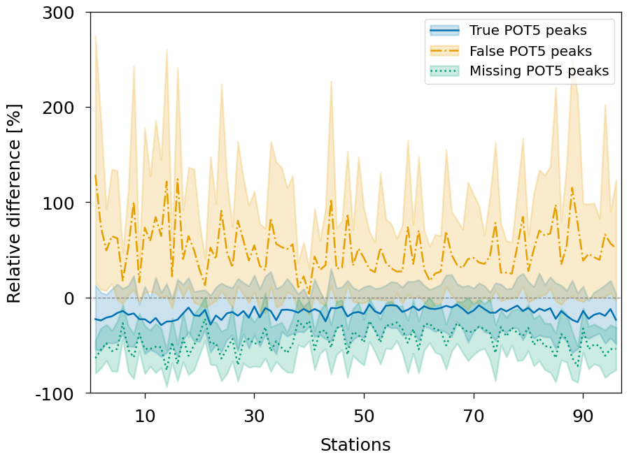
Figure 4 Mean relative difference in magnitudes between observational POT5 peaks and the simulated POT5 peaks from the ERA5-driven simulation. Differences are shown for POT5 peaks, that are present in both time series (true POT5), POT5 peaks which are detected in the ERA5-driven simulation but not in the observations (false POT5), and POT5 peaks which were detected in the observations but not in the ERA5-driven simulation (missing POT5). The shaded areas represent the 10th and 90th percentiles of relative change for the simulated POT5 peaks. The gauges are sorted by their median number of simulated rain-on snow floods shown in Fig. 9.

The adapted definition of widespread floods successfully reproduces most of the detected widespread floods from Uhlemann et al. (2010). During the period from 1952 to 2002, 104 widespread floods were identified in the observations. Out of the 80 widespread floods documented by Uhlemann et al. (2010), only 15 were not identified in our simulations, with most of the missing widespread floods occurring in summer (80 %). Nevertheless, the higher-ranked widespread floods are well represented (Table S1). Moreover, certain events might not be captured due to the differences in the considered gauges and in the definition of widespread floods used in this study and in the study of Uhlemann et al. (2010) (i.e., weighting of gauges by catchment area rather than the length of the river network, as well as different flood thresholds).

The ERA5-driven LSTM simulation appears to represent widespread floods effectively (Fig. 5a). From 1951 to 2015, 127 widespread floods were detected in the observations and 119 in the ERA5-driven simulation. Of the 127 detected floods in the observations, 98 were identified in the ERA5-driven simulation.

Figure 5 Time series of widespread flood frequency for the ERA5-driven LSTM simulation and the GRDC observations (a), temporal distribution of widespread floods for the ERA5-driven simulation and the GRDC observations (b) and seasonal distribution of widespread ROS floods including the 20 highest ranked ROS floods for the ERA5-driven simulation (c).

Most widespread floods occurred between December and March for both the observations and the ERA5-driven LSTM simulation (Fig. 5b). The number of widespread floods between June and October is lower in the ERA5-driven simulation than in the observations. Additionally, the number of widespread floods in summer and autumn is considerably lower than for winter and spring for both time series. The distribution of widespread ROS floods for the ERA5-driven LSTM simulation (Fig. 5c) shows that most widespread floods in Germany are (at least partly) ROS-driven. Furthermore, no widespread ROS floods were detected between August and October for the ERA5-driven simulation. The top 20 highest-ranked ROS floods in the ERA5-driven simulation mainly occurred from January to March with only three of these floods happening in December (2) and April (1).

A comparison of flood-generating processes for individual gauges between the XAI-based interpretation of the ERA5-driven simulation and the attribution by Tarasova et al. (2020b) shows that a time window of 5 d for feature attribution in the XAI-based classification and a minimum IG_ROS of 0.1 as a lower limit for ROS floods yield the best results (Fig. 6). While accuracy and precision achieve optimal results for longer time windows and higher minimum ROS thresholds, recall exhibits the opposite trend. This discrepancy is attributed to the higher proportion of rainfall-driven floods in Tarasova et al. (2020b) compared to the results from the ERA5-driven simulation of this study. Increasing the minimum thresholds for ROS floods increases the number of non-ROS floods, thereby enhancing accuracy and precision. The resulting F1 score, which balances precision and recall, is highest for windows larger than 4 d (as suggested by the correlation in Fig. A1) and lower minimum IG_ROS thresholds. The primary difference from the results from Tarasova et al. (2020b) can be linked to the different data sets used for flood process attribution. They used high-resolution (1 km) precipitation and snowmelt simulated by a regionally calibrated hydrological model (4 km). For a minimum IG_ROS of 0.1 and across all gauges, a snowmelt peak was present in ERA5 for 98 % of all POT5 peaks classified as rainfall-driven according to Tarasova et al. (2020b). This discrepancy likely arises from the coarse resolution of ERA5, which could lead to an inaccurate representation of snowmelt processes, particularly for smaller basins. However, no relationship was found between the F1 score and the basin area.

Figure 6 Comparison of ROS and non-ROS floods according to the classification of Tarasova et al. (2020b) using interpolated observed precipitation and snowmelt simulated by a regionally calibrated hydrological model and the XAI-based classification of floods using ERA5-driven simulations of the LSTM model from this study. Accuracy (a), precision (b), recall (d), and F1-score (d).

The results indicate that the ERA5-driven LSTM simulation and the XAI-based classification of ROS floods can effectively reproduce the findings of previous observation-based studies.

3.1.2 ERA-Interim-driven simulations

The ERA5-trained LSTMs driven by the uncorrected raw output from the CORDEX evaluation runs (RCM-ERA-Interim) fail to accurately reproduce streamflow dynamics in the study area (Fig. 7a), with almost all models performing rather poorly (i.e., negative NSE for nearly all gauges). In particular, the LSTM runs driven by the outputs from HIRHAM5 and ALADIN63 perform very poorly.

Figure 7 Streamflow simulation accuracy of the ERA5-trained LSTM driven by the raw RCM-ERA-Interim (a, d), the RCM-ERA-Interim-trained LSTM (b, e) and the ERA5-trained LSTM driven by the bias-corrected RCM-ERA-Interim (c, f). The top panel shows the mean NSE of the streamflow simulations for each basin. The gauges are sorted by their median number of simulated rain-on snow floods shown in Fig. 9. The bottom panel shows an example of the resulting predicted discharge for 365 time steps of the testing data for the Ingolstadt station. The GRDC observations and the simulated ERA5-driven discharge are added as reference.

In contrast, the LSTMs trained on the uncorrected CORDEX evaluation runs show considerably better performance (Fig. 7b). Although this performance improves considerably, it remains inferior to that of simulations trained and driven by ERA5. While peak flows are underestimated, the overall representation of the streamflow dynamics is greatly improved (Fig. 7e).

Using the bias-corrected output from the CORDEX evaluation runs to drive the ERA5-trained LSTM (Fig. 7c) considerably improves the performance of the streamflow simulation compared to the simulations shown in Fig. 7a. The performance of this simulation is comparable to the performance of the LSTMs trained directly with the evaluation runs instead of ERA5 that was shown in Fig. 7b. Although, the resulting streamflow (Fig. 7f) has more spikes than the simulation shown in Fig. 7e it is a considerable improvement compared to the streamflow displayed in Fig. 7d. These results show the utility of the bias-correction and confirm that the ERA5-trained LSTMs are able to achieve a quality comparable to the LSTMs trained with the evaluation runs. It is important to note that the overall poorer performance was expected compared to the ERA5-driven simulation, because the quantile-delta mapping method does not correct for temporal or spatial shifts of weather patterns. The downscaling of data sets only uses the driving data sets (here: ERA-Interim) as boundary conditions. Considering the large EURO-CORDEX domain, shifts in weather patterns and thus shifts in peak timing and magnitude of the resulting LSTM simulations compared to the observations have to be expected. Although there are more advanced bias-correction methods that address these issues, we prefer quantile-delta mapping because it adjusts the value range of the model data to match that of the training data while maintaining other model characteristics, particularly in the context of potential future climate changes. Furthermore, the potential impact of minor spatial and temporal shifts in weather patterns is likely to be rather small in the context of widespread winter floods.

3.1.3 Historical period of RCM-GCM-driven simulations

To confirm and evaluate the simulation quality of the climate projections, the climatology for the REF period is compared with GRDC observations for the 31 GCM-RCM-driven and ERA5-driven simulations. The ensemble median annual streamflow closely aligns with the GRDC observations (Fig. 8). For most gauges, it is overestimated by up to 15 % for the ensemble median and 25 % for the 90th percentile. Only at eight gauges is the mean streamflow underestimated in the median, and to a lesser extent. In contrast, for the ERA5-driven simulation, the mean streamflow is underestimated in more cases than it is overestimated.

Figure 8 The climatological difference for mean streamflow and mean annual maxima between the ensemble of the RCM-GCM-driven simulations and the GRDC observations, and between the ERA5-driven simulation and the GRDC observations. The shaded areas represent the 10th to 90th percentiles of the GCM-RCM ensemble. The gauges are sorted by their median number of simulated rain-on snow floods shown in Fig. 9.

The mean annual maxima are consistently lower by up to 50 % for the ensemble median and are only overestimated for a few gauges within the 10th to 90th percentiles. The mean annual maxima for the ERA5-driven simulation show even higher underestimation than those for the ensemble median. Overall, the ERA5-trained LSTMs can produce realistic streamflow when driven by climate projections.

3.2 Projected changes for rain-on-snow floods

In the following section, we present the changes in ROS floods for the four examined time periods. These changes are analyzed first separately for the individual gauges and then at a widespread, multi-catchment scale for the four major river basins of the Rhine, Danube, Elbe, and Weser rivers. The figures shown in this section focus mainly on the changes in the GCM-RCM ensemble median. Figures illustrating the changes for the individual models can be found in the Supplement.

3.2.1 Individual gauges

The results and trends of ROS floods for the individual gauges are shown in Fig. 9. Figure 10 (Figs. S2 and S3) adds spatial context for the changes projected for the ensemble median for the periods 2041–2100 (1981–2040 and 2011–2070) and displays the significance of the results. For the 1981–2040 period, there is an overall slight increase in ROS flood frequency for the ensemble median (Figs. 9a and S2a). Starting in the 2011–2070 period, the ROS flood frequency decreases for most gauges (Fig. S3a), while 13 gauges experience an increase. In particular, for the 2041–2100 period, some gauges exhibit an extreme increase in numbers, whereas for most gauges, a moderate to high decrease is projected (Fig. 9a). The gauges with an increasing number of ROS floods are located in the northwestern part of the Danube River Basin, as well as the midwestern part of the Elbe River Basin (Fig. 10a). In these basins, some catchments are associated with higher elevations compared to the Rhine and Weser River basins. Apart from one gauge in the Danube River basin that shows an increase of up to 113 % for the ensemble median, the increase for all other gauges falls within the range of −60 % and +80 %. For the 10th to 90th percentiles these values range from −78 % to +175 % (Fig. 9a). The changes in ROS-flood number are significant at 70 % of all gauges for the 2041–2100 period.

Figure 9 Number of ROS floods and their properties for 4 time periods. The top panel shows the number of ROS floods (a), the XAI-based snowmelt importance IG_ROS (b), the mean normalized rank (c), the maximum normalized rank (d) and the mean ROS flood date (e) for the GCM-RCM ensemble median for the reference period REF. The shaded areas represent the 10th to 90th percentile of the RCM ensemble. The lower panels show the relative changes for 3 future time periods with regard to the reference period. The gauges in all panels are sorted by the median number of ROS floods.

Figure 10 Changes in the number of ROS floods (a), the IG_ROS (b), the mean normalized rank (c), the maximum normalized rank (d) and the mean date (e) at all gauges for the GCM-RCM ensemble for the future period 2041–2100 with regard to the reference period. Significant changes are marked with an x.

For the REF period, snowmelt is 2–4 times more important for the LSTM predictions than liquid precipitation during ROS floods in the ensemble median (Fig. 9b). The IG_ROS values are generally lower for gauges with a higher ROS flood frequency. The importance of snowmelt significantly decreases for all gauges throughout all periods, by up to 57 % for the ensemble median and 78 % for the 10th to 90th percentiles for the 2041–2100 period.

Figure 9c shows ensemble median of the mean normalized rank of ROS floods. If flood severity was distributed evenly for all periods, the mean rank in each period would be close to 0.5. Any larger deviation indicates that floods are more or less severe during a specific period. The overall sensitivity of this measure is highly dependent on the total number of ROS floods during a period. This limits the ability to compare the numbers of absolute change in mean rank between different gauges and different GCM-RCM models. However, it is possible to determine whether there is a change and in which direction it points. For all future periods, the mean normalized rank increases for most gauges, with a generally higher increase for distant futures for the ensemble median. However, the spread of the models increases considerably after the 1981–2040 period. There are only a few individual gauges that experience a decrease in mean rank (Fig. 10c). For the 2041–2100 period, these changes are significant for about 60 % of all gauges.

Similarly as for the mean rank, the maximum rank also has its limitations due to the different numbers of ROS floods. As the highest rank is represented by the value 1, it is possible to determine in which period the strongest flood occurred. The exact distance in terms of ranks to the other periods is not easily visible in this representation, but in the same way as for the mean rank it can display the direction of the trend. The maximum rank (Fig. 9d) does not reach the value of 1 for the 10th to 90th percentiles in the REF period for any of the gauges. This means that the most severe flood is always found within one of the future periods. While for the 1981–2040 period the maximum rank appears to be higher for most of the gauges, more gauges also see a decrease in the maximum rank for the 2011–2070 period, and especially for the 2041–2100 period. The eastern part of the Rhine, western part of the Danube, middle to northern parts of the Weser, and western part of the Elbe River basins contain most of the gauges with a projected increase in maximum flood rank for the 2041–2100 period (Fig. 10d). Gauges with a projected decrease in maximum flood rank are mainly located in the middle and western parts of the Rhine, the southern part of the Weser, and the northeastern part of the Danube River basins. For the 1981–2040 period, the maximum rank is always at least as high as for the REF period (Fig. S2d). The pattern of the projected changes for the 2010–2070 period (Fig. S3d) appears similar to the changes for the 2041–2100 period. However, more of the gauges still show an increase in maximum flood rank, and the projected decreases in maximum flood rank are less pronounced. The changes are only significant for about 40 % of the gauges for the 2041–2100 period.

There is a clear pattern for the change in average ROS flood timing, with earlier occurrences in the south and east of Germany and later occurrences in the northwest for the ensemble median for the 2041–2100 period (Figs. 9e and 10e). In central Germany, there is a transition zone with only minor shifts in mean ROS flood date. The average time changes for the ensemble median are generally very small, within ±10 d for the 2041–2100 period, but can be as large as ±25 d for models within the 10th and 90th percentiles. The same pattern is already visible for the 1981–2040 and 2011–2070 periods. However, the changes are not significant for most of the gauges.

Generally, the patterns of projected changes from most of the climate models align with the ensemble median (Figs. S4–S8). In terms of ROS frequency, most models agree on an increase in the Danube River basin and in the western parts of the Elbe River basin, although to varying extents. Some models also project an increase in the Weser River basin, which is not reflected in the ensemble median. In some cases, an extreme increase in ROS flood frequency across large parts of Germany is projected. This behavior is particularly evident in the CNRM-CERFACS-CNRM-CM5-driven RCMs and the GCMs downscaled by the KNMI-RACMO22E model. With regard to changes in the importance of snowmelt, all models agree on a decreasing trend. For most models, some individual gauges, which are spatially heterogeneously distributed within all major river basins, show an increasing trend. The patterns of changes in mean and maximum rank also differ from model to model, but the magnitude of changes is similar across simulations. For flood timing changes, the patterns for many models again appear very similar to the ensemble median. However, there are also models which project a shift to later timings for all of Germany or the opposite. Possible reasons for the differences in trends are discussed at the end of this section.

3.2.2 Widespread floods

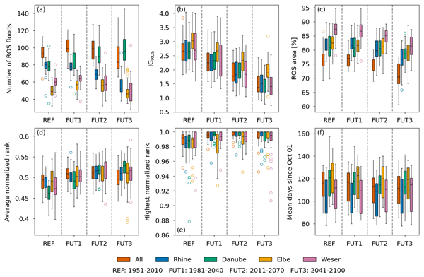
A similar picture to that projected for the individual gauges emerges for the widespread floods. For the Rhine River basin, the number of ROS floods is decreasing throughout all periods (Fig. 11a). The Elbe River basin experiences an increase until the 2011–2070 period, before facing a decrease in ROS flood numbers in the 2041–2100 period. For the Weser River basin, this decline begins already after the 1981–2040 period. Only the Danube River basin shows an increasing trend in ROS flood frequency throughout all periods. When all regions are combined, the numbers increase until the 1981–2040 period and then decline. For the Danube River basin and the combined basins, the model spread increases significantly towards the distant future periods. The projected changes for the 2041–2100 period are significant (P<0.05), except for the Elbe River basin, due to the decline in ROS numbers after the 2011–2070 period. However, for the Elbe River basin, the change for the 2011–2070 period is significant. The exact p-values are shown in Table S2.

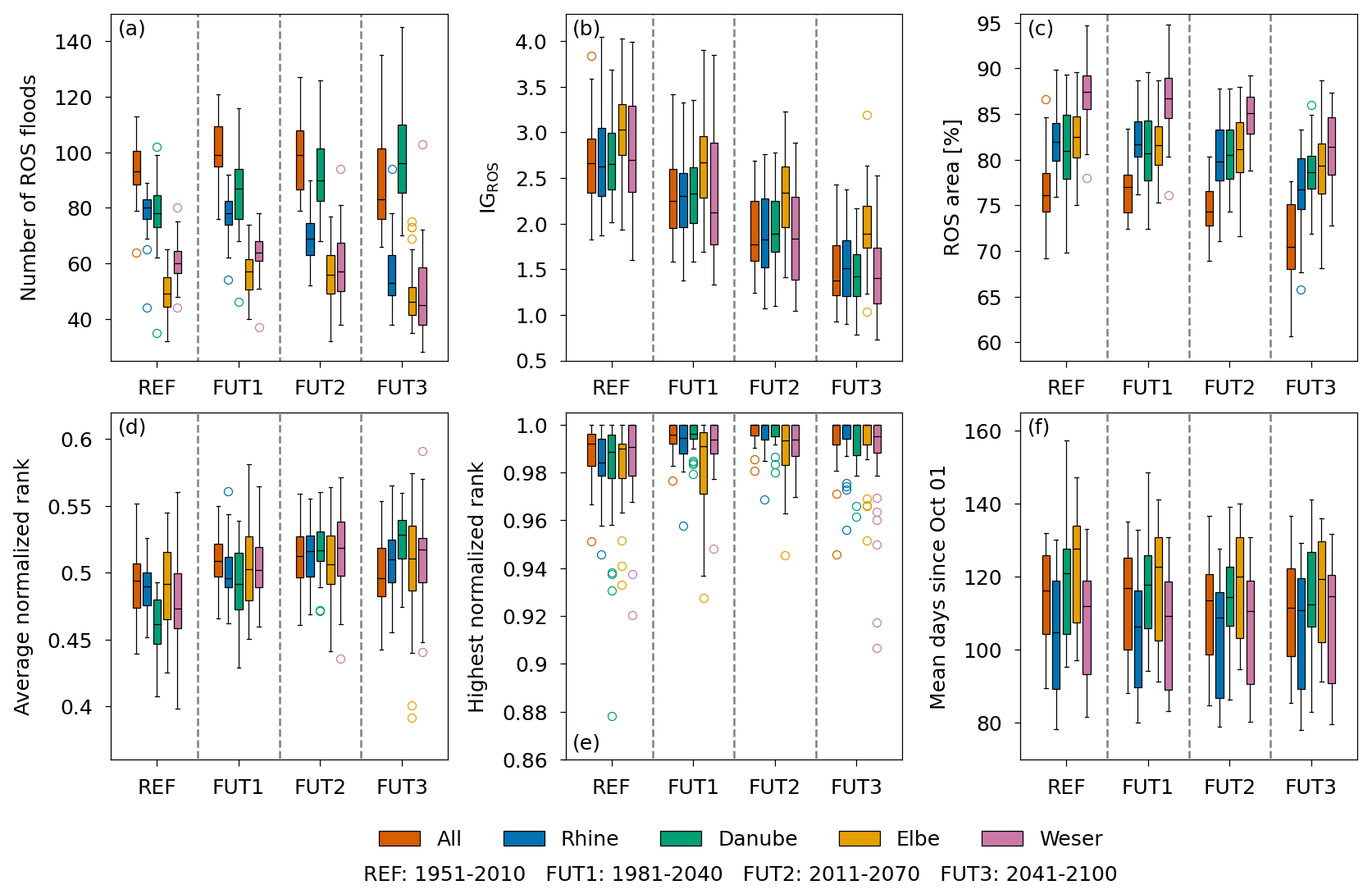
Figure 11 ROS flood properties for the RCM ensemble for the 4 time periods REF, FUT1 (1981–2040), FUT2 (2011–2070) and FUT3 (2041–2100). The number of widespread ROS floods (a), the mean importance of snowmelt IG_ROS (b), the fraction of the mean area affected by ROS floods (c), the mean normalized rank (d), the maximum normalized rank (e) and the mean ROS flood date (f). The boxes represent the 25th to 75th percentile with the median as line within the box. The whiskers show 1.5 times the inter quartile range. Outliers are shown by the colored circles.

In Fig. 12b, the decreasing trend for the Rhine, Weser, and Elbe River basins begins around 2040 to 2050. Until the 1990s, the numbers are increasing and remain stable until 2040. At the same time, the number of non-ROS widespread floods (Fig. 12a) is increasing for all basins except the Danube River basin throughout the entire time series. The numbers for the Danube River basin start to increase only after the 2090s. In total, the number of all widespread floods is increasing throughout the time period, but the fraction of ROS floods decreases from 60 % (Elbe) and 80 % (all other basins) for the ensemble mean to 40 % (all basins except Danube). The ROS fraction for the Danube River basin remains high at 80 %. Although ROS-events are an important driver of floods in Germany, they are not the dominant driver. Compared to Tarasova et al. (2023), who found that ROS floods account for 20 %–30 % of total mean annual floods at streamflow gauges Germany, we find a much higher share of up to 80 % in the ensemble median for widespread floods. The main reason for that is that, according to Uhlemann et al. (2010), widespread floods in winter account for 66 % of total widespread floods in Germany. In our simulations this share is even larger due to the underestimation of summer floods. Additionally, the number of widespread ROS floods is highly dependent on the area threshold described in Sect. 2.4.

Figure 12 Rolling 10-year sum of non-ROS widespread floods (a), ROS widespread floods (b), and the fraction of ROS floods with respect to all widespread floods (c) for the Rhine, Danube, Elbe, and Weser River basins as well as for all basins combined during all months.

The IG_ROS value (Fig. 11b) is significantly decreasing for all basins, dropping from a median between 2.75 and 3 in the REF period to a median between 1.5 and 2 in the 2041–2100 period, indicating a clear trend towards a more rain-driven ROS floods. In all periods, ROS floods in the Elbe River basin are more snowmelt-driven compared to those in the other basins. Alongside the decreasing trend in the importance of snowmelt, the proportion of the flood area affected by ROS is also declining (Fig. 11c). Most basins experience a reduction of 5 to 10 percentage points in the median until the 2041–2100 period. During the 1981–2040 and 2011–2070 periods, the ROS-affected area remains relatively stable for the Rhine, Danube, and Elbe River, only starting to decline in the 2041–2100 period. The ROS-affected area for the Weser River basin is already decreasing during the 2011–2070 period. For the Danube River basin, this trend is not significant (p=0.052). Because of the high number of widespread floods in the Rhine and Danube basins and the low numbers of widespread floods in the Elbe and Weser basins, the relative affected area of the combined basins is lower than for the individual basins.

For the mean and maximum normalized rank (Fig. 11d and e), an increase is projected at least until the 2011–2070 period. The mean rank for the 2041–2100 period shows a further increase for the Danube River basin and a slight decrease for the Rhine River basin as well as for all basins combined. The maximum rank displays higher values for all future periods compared to the REF period. However, they are very similar to one another, except for the Elbe River basin, which exhibits a wide model spread, particularly for the 1981–2040 period. In terms of model spread, for the 2041–2100 period, the maximum rank appears to be lower for some models than for the 2011–2070 period. The changes in mean rank are significant until the 2011–2070 period for all major basins. For the 2041–2100 period, the changes are not significant for the Elbe River basin due to the larger model spread and for all basins combined due to the decrease in rank. Except for the Weser River basin, the changes in maximum rank are significant for the 2041–2100 period. While the exact amount of the increase in magnitude cannot be determined solely by considering rank as a measure, the trend towards stronger ROS floods is clear.

The trend for the average timing of ROS floods (Fig. 11f) is not as clear as for the other characteristics. For the Danube and Elbe River basins, the ensemble median projects a shift of 10 d to earlier dates. In contrast, the Weser River basin shows almost no change, while the Rhine River basin is projected to experience a shift to later dates. However, the model spread for the 25th to 75th percentiles remains similar, and there is no significant difference between the ensemble across all periods.

This is also reflected in the change in seasonality of widespread ROS floods. The seasonality of ROS floods for the REF period is similar to that of the ERA5-driven simulation, but with a maximum in January instead of February. All basins exhibit strong seasonality with almost no ROS floods from May to September in the median, except for the Danube River basin, where ROS floods occur frequently during May and September. For the Elbe River basin, the seasonality is weaker, with many ROS floods occurring in February and March. In some models within the 10th and 90th percentiles, ROS floods can be found in summer, especially for the Danube River basin. For the 2041–2100 period, the seasonality tends to become slightly stronger for all basins, with the largest change occurring in the median for the Elbe River basin and for the Danube River basin when considering individual models from the 10th to 90th percentiles.

Diverging trends and discrepancies among some of the individual models are also apparent on the widespread scale. This is most evident in the frequency and in the maximum rank of widespread ROS floods. As with the individual gauges, the reasons for the diverging trends will be discussed at the end of the section.

In Fig. 12, the time series for the number of ROS floods shows distinct periods with a high number of floods and periods with fewer floods. This behavior was previously noted by Tarasova et al. (2023), who investigated the change in flood-generating processes using observations between 1960 and 2010 in Europe. Figure A2 shows the time series of ROS widespread floods grouped by the driving GCMs of the climate simulations. While the different RCMs show some contribution to the frequency of ROS widespread floods, the general trend and periods of high and low amounts of ROS floods are dominated by the driving GCM. These periods of high and low numbers of ROS widespread floods appear in both the historical period and the future, indicating that persistent periods of many ROS floods may still be present in a future warming climate.

Previous studies identified flood-rich and flood-poor periods in observational data (e.g., Schmocker-Fackel and Naef, 2010; Villarini et al., 2013; Merz et al., 2016; Fischer et al., 2023), which appear to be primarily caused by catchment memory effects rather than decadal climate variability (Schmocker-Fackel and Naef, 2010; Merz et al., 2016). However, for the USA, Villarini et al. (2013) observe a correlation between flood-rich and flood-poor periods and large-scale climate indices such as the North Atlantic Circulation (NAO)-Index. Note that these studies mainly focus on flood events with a high magnitude. In this study, flood events with a variety of flood magnitudes are considered. However, the attribution of the flood-rich and flood-poor periods found in this study to the decadal variability of large-scale climate drivers is supported by studies that have identified a correlation between the frequency of ROS events and the NAO and the Arctic Oscillation (AO) (e.g., Cohen et al., 2015). Additionally, other studies attribute lower snow heights to a positive phase of the NAO (e.g. Hurrell, 1995) and find larger snow amounts primarily during negative phases of the NAO (e.g. Krug et al., 2020). Furthermore, Comas-Bru and McDermott (2014) point out the importance of the Eastern Atlantic pattern (EA) and the Scandinavian pattern (SCA) on the winter climate conditions in Europe. The dominant characteristics of the GCMs further support a correlation of ROS flood frequency and NAO and AO, since the GCMs are initialized differently and are in different phases of large-scale climate patterns such as NAO and AO (note that in Fig. A2, the MPI-M-MPI-ESM-LR-GERICS-REMO2015 driven LSTM simulation was excluded, because a different GCM ensemble member (r3i1p1 instead of r1i1p1) was used and thus the phases did not match) (Taylor et al., 2012).

This motivates further investigation of a generating-process-based relationship between flood frequency and large-scale climatic drivers without dependence on flood magnitude.

3.3 Change of atmospheric variables

Changes in ROS events, as a flood-generating process, can be attributed to changes in rainfall and snow accumulation (Freudiger et al., 2014). Figure 13 shows the mean relative changes in snow amount, snowmelt, snowfall and liquid precipitation from the model ensemble as described in Table 1, for the 2041–2100 period relative to the REF period (See Figs. S9 and S10 for the periods 1981–2040 and 2011–2070). For all snow-related variables, there is a clear decrease in both the mean annual maxima and the maxima over the specified time periods. The changes in the mean annual maxima are more pronounced, as very rare extreme events are still projected to occur in the future.

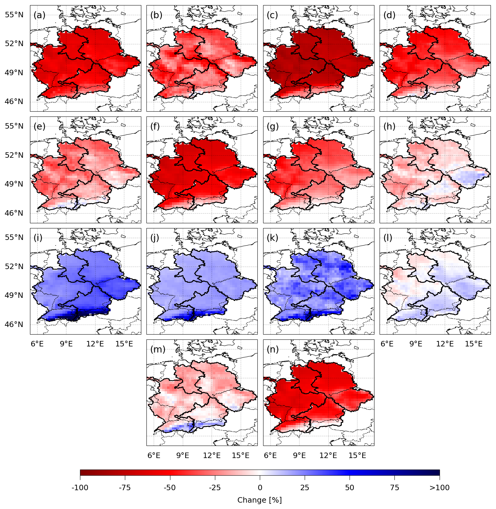
Figure 13 Ensemble mean of relative changes of selected atmospheric variables for 2041–2100 compared to the REF period. Mean annual maximum snow amount (a), maximum snow amount (b), mean annual snow days (snow amount > 15 mm SWE) (c), mean October to May maximum 5 d snowmelt (d), maximum October to May 5 d snowmelt (e), mean October to May snowfall amount (f), mean October to May maximum 5 d snowfall amount (g), maximum October to May 5 d precipitation amount (h), mean October to May liquid precipitation amount (i), mean October to May maximum 5 d liquid precipitation amount (j), maximum October to May 5 d precipitation amount (k), mean ROS water (5 d sum of liquid precipitation and snowmelt if ROS conditions are met) (l), maximum ROS water (5 d sum of liquid precipitation and snowmelt if ROS conditions are met) (m) and the number of times the ROS conditions are met (n). The ROS conditions are met if both ratios of the 5 d sum of liquid precipitation and snowmelt are smaller than 0.1.

The mean annual winter snowfall is projected to decrease across the entire study area, which will also impact annual maxima in snow amount and snowmelt. Notably, the annual number of snow days with a snow cover exceeding 15 mm SWE is decreasing significantly. The smallest projected decrease is found in the Alps for all snow-related variables. For the period maxima, additional regions outside of the Alps show lower decreases or, in the case of 5 d snowfall, even an increase. These regions are located in the Czech and midwestern parts of the Elbe River basin, the Danube River basin, and the northern and eastern parts of the Rhine River basin. In these areas, some models project extremes that exceed a 100 % increase compared to the REF period.

In contrast to the snow-related variables, liquid precipitation is projected to increase in winter, both in terms of mean values and extremes, exceeding 100 % in the Alps. The mean 5 d ROS water (i.e. the 5 d sum of liquid precipitation and snowmelt) is therefore only decreasing in certain areas of the Rhine River basin and the northern parts of the Weser and Elbe River basins. While ROS water extremes are decreasing, this decline is not as pronounced as that of the snow-related variables. The increase in liquid precipitation can compensate for most of the loss in snowmelt. However, ROS events (defined here as events with ratios of 5 d liquid precipitation and 5 d snowmelt < 0.1) are significantly declining. This is also in line with the decline in ROS frequency in observations (Freudiger et al., 2014) and a projected decline in ROS frequency for a future SSP5-85 scenario (Maina and Kumar, 2025). However, in their study, the decrease in the Alps is smaller than in the lower-elevated regions.

Although the trends of the variables generally align with the trends in ROS properties, such as a decrease in the importance of snowmelt, a decline in ROS frequency at most gauges, and a slight increase in mean severity for the ensemble median, this alignment is not apparent for the extremes. Outside of the Alps, there are no regions showing an increase in maximum 5 d ROS water for the ensemble median. Additionally, for the individual models, the patterns of projected changes in maximum ROS flood rank do not correspond with the projected changes in maximum 5 d ROS water. Increase winter precipitation may lead to more frequent soil saturation and potentially higher mean streamflow, which could enhance extreme flood events.

The diverging trends in ROS floods among the individual models may seem surprising initially, as all trends in the variables shown in Fig. 13 (except for the extreme values for each period) share the same direction and a similar magnitude (Figs. S11–S24). However, there are large differences in the snow amount and the melting seasons. While the general patterns of snow and precipitation distributions align well, these differences especially lead to high variability of the conditions during the REF period and the projected future values for the 2041–2100 period. For example, the RCMs driven by CNRM-CERFACS-CNRM-CM5 and the GCMs downscaled by KNMI-RACMO22E produce a high number of ROS events in the REF period (Fig. S25) and maintain high numbers in the 2041–2100 period (Fig. S26). The relative trend is similar to that of the other models (Fig. S24). The modeling process of snow is very complex and depends on a complex model chain consisting of many parts, such as the land-surface model of the RCM and its parameterizations, and the forcing data of these land-surface models that is produced by the RCMs. Additionally, the forcing data of the GCMs can introduce biases, although they can partially get compensated by the RCMs (Sørland et al., 2018). A cold bias in an RCM will likely make the land-surface model produce more snow. However, different land-surface models may have a different sensitivity to such biases. A recent study by Risto et al. (2025) shows the sensitivity of snow mass and snow cover produced by a land-surface model to perturbations in the forcing precipitation and the albedo in seasonal forecasts. Variations in both parameters can greatly affect seasonal snow amounts. Terzago et al. (2017) find that RCMs used for downscaling of ERA-Interim and CMIP5 GCMs heavily overestimate the snow pack over the higher-elevated Alpine region, but underestimate the snow pack in the lower-elevated parts of the region. They explain this overestimation with cold biases or wet biases in the forcing coming from the RCMs or, if no biases were apparent in the forcing, to the snow scheme of the land-surface model and the spatial resolution of the RCMs. They also highlight the large spread of the models in terms of snow amount. However, all RCMs agree on the reduction of snow amount in future projections. Although the atmospheric input for the LSTM is bias corrected and all variables are within a similar range, there are large differences in variability of daily rainfall and especially in the melting season. In particular, the melting seasons in KNMI-RACMO22E and CNRM-ALADIN63 RCMs start 30 to 50 d later compared to GERICS-REMO2015. For threshold processes such as ROS floods even small changes in the snow amount or the rainfall can make the difference for it beeing classified as snowmelt or rainfall event.

The extreme increase in ROS frequency of the CNRM-CERFACS-CNRM-CM5 GERICS-REMO2015 setup can be attributed to a very high frequency of snowmelt floods in the REF period (Fig. S27), which transform to ROS floods in a warming climate. Changes in ROS properties resulting from such extreme changes in ROS frequency are most likely due to statistical reasons.

For the other models, the explanation is not as straightforward. However, RCMs driven by the same GCM and GCMs driving the same RCM often exhibit a similar behavior.

The high variability between climate models in terms of projected flood changes has been highlighted in numerous other studies (e.g., Smith et al., 2014; Camici et al., 2014). Sezen et al. (2020) addressed this issue concerning changes in ROS frequency and severity. They also emphasize that in addition to changes in meteorological conditions, factors not included in the GCMs and RCMs, such as changes in land use, could further influence future ROS floods.

For recent CMIP6 global climate projections, the less pessimistic SSP3-7.0 emission scenario is used as the high-impact scenario to drive the RCMs in the CORDEX. Under this emission scenario, the projected changes of the 2041–2100 period could potentially be lower in the CORDEX CMIP6 ensemble and may resemble the changes found for the 2011–2070 period at the end of the century. (Maina and Kumar, 2025) highlight that during a transition phase with decreasing snow cover and increasing precipitation, ROS events can potentially trigger large amounts of snowmelt. In a less pessimistic scenario, the duration of such a transition phase is potentially longer and therefore poses an increased risk of severe ROS floods.

4 Conclusions

In this study, we analyzed the changes in frequency, severity, and properties of rain-on-snow (ROS) floods in Germany. We used 31 combinations of global and regional climate models to simulate future streamflow under the RCP8.5 high-emission scenario at 96 river gauges in Germany, using a Long Short-Term Model that was trained to reproduce past streamflow observations when driven by the ERA5 reanalysis. The model demonstrated an accurate representation of flood timing, and its ability to simulate flood events, despite generally underestimating their severity, warranted the use of a novel explainable artificial intelligence technique to identify floods generated by the ROS process.

Our findings indicate a decline in the frequency of ROS floods at the majority of individual study gauges with only a few projected increases win the Danube and Elbe River basins. Notably, the Danube region is the only area showing a steady increase in widespread ROS floods in the future.

Overall, ROS floods are becoming more rainfall-driven, with a corresponding decrease in the contribution of snowmelt for all individual gauges and for widespread floods in the study area. Consequently, the area of widespread floods affected by ROS is also declining.

The mean rank (as a representative of the mean severity within a time period) of widespread ROS floods shows an increase until the period from 2011 to 2070, while the maximum rank (as a representative of the highest severity within a time period) of ROS floods increased from the period from 1951 to 2010 towards the period from 1981 to 2040, subsequently remaining stable in more distant future periods. The maximum rank of ROS floods is projected to be higher for all basins in all future periods. Additionally, the mean rank of ROS floods increases for almost all individual gauges. However, the maximum rank increases only in most of the western Danube basin, the western Elbe, and the middle to northern Weser basin and decreases in most of the Rhine basin.

This decreasing importance of snowmelt, along with the declining ROS frequency and the increasing mean flood rank, is reflected in changes in the mean values of the corresponding atmospheric variables. While snow amount and snowmelt decrease, liquid precipitation generally increases from October to May, compensating for the loss of snowmelt. Additional factors such as increased soil moisture and higher mean winter streamflow are likely contributing to the increase of the maximum rank of ROS events.

There is a considerable variability between the models regarding the trends of ROS floods, which is related to complex model chains of the individual climate models leading to different variability of precipitation and snowmelt and different timings of the melting seasons. For threshold-based processes, even small changes in the involved variables, can lead to a different interpretation of the processes. This highlights the necessity for ensemble-based assessments for understanding and projecting local changes in future flood-generating processes.

Appendix A: Appendix

Table A1 Climate simulations from the CORDEX CMIP5 ensemble.

All simulation data can be downloaded at https://esgf-metagrid.cloud.dkrz.de/.

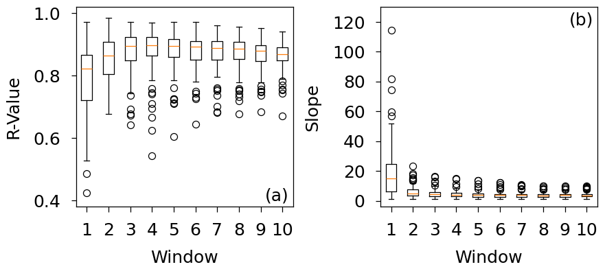
Figure A1 Correlation (a), and slope of the regression line (b) for the XAI-based IG_ROS value and the ratio of snowmelt and liquid precipitation of ERA5 for ROS POT5 peaks using different time windows for the XAI-based classification.

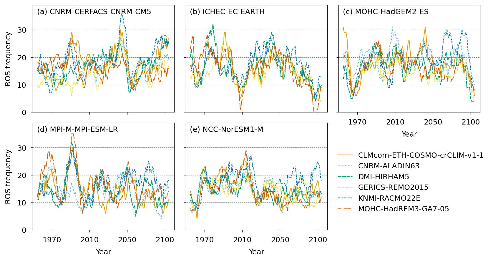
Figure A2 Rolling 10-year sum of ROS widespread floods detected in the streamflow simulations of the individual climate models for all basins combined during all months. The different panels show the number of ROS widespread floods for different driving GCMs. (a) CNRM-CERFACS-CNRM-CM5, (b) ICHEC-EC-EARTH, (c) MOHC-HadGEM2-ES, (d) MPI-M-MPI-ESM-LR, and (e) NCC-NorESM1-M. The CCCma-CanESM2 and MIROC-MIROC5 GCMs, and the MPI-M-MPI-ESM-LR-GERICS-REMO2015 simulation were excluded.