Persistence of scour at bridges using stochastic simulations

The stochastic and deterministic properties of the scouring process at bridges are analysed by coupling synthetic streamflow generations with a scour and fill model considering the upstream sediment supply. Streamflow was generated using the asymmetric moving-average (AMA) scheme that preserves the Hurst-Kolmogorov (HK) dynamics, the second-order dependence structure, time asymmetry, and the first four statistical moments of the marginal distribution. Stationarity, homogeneity, and ergodicity of the streamflow and scouring processes were assumed. Monte Carlo analyses covered 12 000 realisations for each of the three considered scenarios with different upstream sediment supply. Extreme scour events were assessed using annual maxima with GEV fitting and compared against the equilibrium scour. The dependence structure was identified with the climacogram and climacospectrum stochastic tools and fitted with a filtered HK model (FHK-CD). The obtained results show a multi-scale dynamics of the scouring process with rough and weak persistent behaviour (M≈0.40; H≈0.60), while envelopes span from antipersistent to strongly persistent scour regimes (H  up to  ≈0.86) depending on the upstream sediment supply. It is worth noting that the upstream sediment supply reduced the envelope variability and modified the extreme scour values. Additionally, synchronisation between extreme events of streamflow and scour showed a weak correspondence (Critical Success Index ≈0.15–0.60), indicating that streamflow extremes do not systematically translate into scour extremes. Finally, scour depths with a given return period (computed from scour time series) increase with upstream sediment supply.

1 Introduction

Scour continues to be a leading cause of infrastructure damage worldwide. Local scour – occurring at pipelines, bridge piers, groynes, and abutments – is a highly time-dependent process driven by non-linear interactions among the fluid, the turbulent flow, the sediment dynamics, and the geometry of the obstacle opposing the flow (Breusers et al., 1977; Dargahi, 1990; Raudkivi, 1986). The interplay between scour and fill results in significant temporal variability in scour depth and bed level (Lee et al., 2021; Link et al., 2020; Lu et al., 2008; Pizarro et al., 2020), making the accurate prediction of extreme scour depths a crucial aspect of bridge safety. Current design practices typically adopt enveloping equilibrium scour curves based on the magnitude of extreme streamflow events, which usually have return periods of 100-200 years (see, e.g.: Arneson et al., 2012; Chilean Ministry of Public Works (MOP), 2020; German Association for Water, Wastewater and Waste (DWA), 2020; Melville and Coleman, 2000). Although these approaches provide conservative safety margins (Rifo et al., 2022; Shahriar et al., 2021), failures still occur under scattered peak flood events (Cook et al., 2015), evidencing the stochastic nature of scouring processes and the limitations of adopted design philosophies.

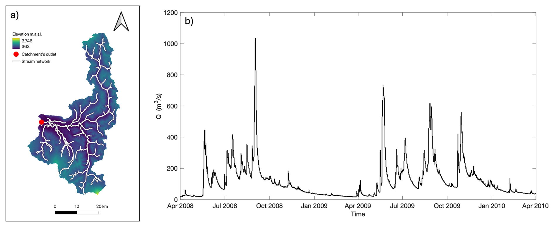
Figure 1 Analysed catchment (a) and streamflow data visualisation (b) of two hydrological years (2008 and 2009). Notice that the hydrological year starts on the 1 April.

From a natural-hazards perspective, bridge scour is a hydrologically driven erosional hazard through which floods can progressively scour foundations and, in many cases, cause structural failure and disruption of transport networks (Cook et al., 2015; Tubaldi et al., 2022). Unlike hazards characterised solely by the magnitude of an individual event, scour is a cumulative, time-dependent process governed by the temporal sequence of stream flows, sediment transport, and the alternating erosion and filling of the scour hole. Consequently, similar flood peaks may produce different scour responses. Characterising the variability, persistence, and return levels of scour is therefore relevant to natural-hazard assessment, as it provides the hazard information required for subsequent evaluations of bridge vulnerability and risk as well as supporting monitoring, maintenance, and mitigation strategies.

Hydrological processes exhibit intrinsic variability and persistence at multiple temporal scales (Dimitriadis et al., 2021; Koutsoyiannis, 2010, 2011). Long-term persistence (LTP) clusters extreme events over decades, substantially increasing uncertainty in design (Koutsoyiannis and Montanari, 2007), while short- and intermediate-term persistence (STP and ITP) control variability at local and seasonal scales. These properties challenge the reliability of return-period-based designs, which assume that extreme events are independent of each other. Moreover, streamflow records are often sparse, difficult to measure during floods, and subject to errors in rating curves, further propagating uncertainty in scour estimates.

Probabilistic approaches have therefore been proposed to incorporate hydrologic uncertainty into scour predictions (Brandimarte et al., 2006; Johnson, 1992). Monte Carlo frameworks have been utilised to integrate flow variability with equilibrium scour equations, providing practical guidance for engineering design. However, these methods remain time-independent, neglecting the inherently dynamic nature of scour. Time-dependent models (such as SRICOS, Briaud et al., 2007) have enabled the simulation of scour evolution under variable hydrographs; however, their lack of representation of sediment deposition leads to unrealistic continuous and monotonically increasing scour growth. More recently, advanced models (see, e.g., Flores-Vidriales et al., 2022; Link et al., 2017, as well as Pizarro et al., 2017a with fill model extension) have incorporated both time dependence and depositional processes, opening the possibility of more physically consistent probabilistic frameworks.

Despite these advances, fundamental research questions remain unresolved: What are the stochastic and deterministic properties of the scouring process? Is time asymmetry a significant concern for bridge scour? Is there a direct correspondence between extreme events of streamflow and scour? A flood event associated with a given return period can be assumed to produce a scour depth characterised by the same return period? Stochastic frameworks that consider hydrological variability, capture time asymmetry, and generate long synthetic scour records can contribute to answering these questions.

The present study addresses the aforementioned knowledge gaps by coupling stochastic simulations of river streamflow with a deterministic scour and fill model that accounts for upstream sediment supply. Streamflow time series are generated using the asymmetric moving average (AMA) scheme, which parsimoniously preserves the first four statistical moments, second-order dependence structure, and time asymmetry. These are then propagated through time-dependent scour models to produce synthetic scour series suitable for extreme value analysis. We evaluate the stochastic properties of the scouring process, assess the role of time asymmetry, and quantify uncertainty in design scour estimation. The rest of this document is organised as follows: the case study and methodology for stochastic and pier-scour analysis are presented in Sect. 2; Sect. 3 shows the results; Sect. 4 addresses strengths and limitations, whereas conclusions are provided at the end.

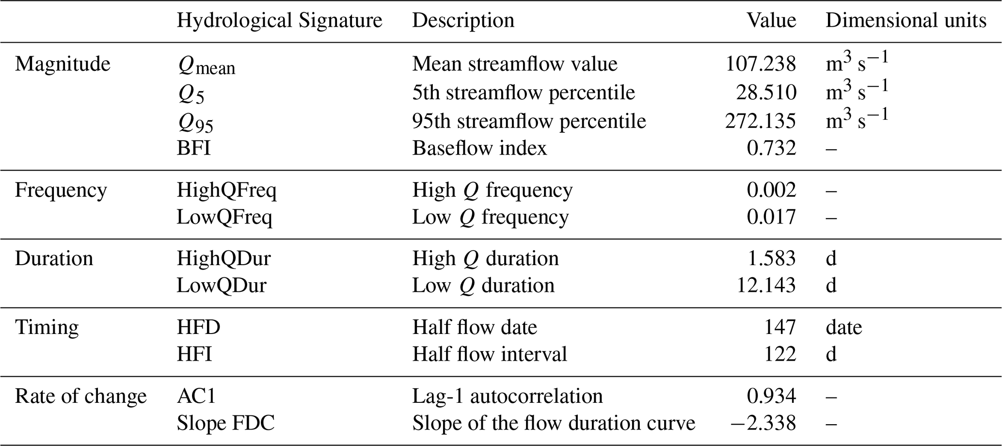
Table 1 Hydrological signatures characterising the magnitude, frequency, duration, timing, and rate of change of streamflow.

2 Methods

2.1 River streamflow data and bridge case study

Streamflow data from the “Trancura River before the Llafenco River” gauging station was selected (ID: 09414001) due to the near-natural hydrologic regime and data monitoring frequency. Its catchment is located in Southern Chile (lat: 39.33° S, lon: 71.77° W), and considers only near-natural flow conditions, neither altered through hydropower plants nor lake regulation or water transfer. The catchment area is 1380 km², the mean annual precipitation is 2853 mm, and the aridity index is 0.3. The maximum, mean, and outlet catchment elevations are 3746, 1147, and 363 m a.s.l., respectively. The gauging station covers several decades of monitoring, but the period from 23 November 2001 to 31 January 2024 was selected for analysis due to its hourly measurement frequency (resulting in a total of 181 038 non-empty values). This temporal scale is crucial to characterise hydrological dynamics in terms of magnitude, frequency, duration, timing, and rate of change. Additionally, the computing of the effective flow work parameter (W^*, see Sect. 2.3.1) is very sensitive to this time discretisation, in which a more accurate hydrograph representation leads to a more accurate calculation. Figure 1 shows the analysed catchment and two hydrological years of stream flows, whereas Table 1 shows 12 hydrological signatures that characterise hydrological dynamics.

The case study consists of a two-span bridge (60 m long) with one submerged pier (the bridge span is 30 m). The bridge pier is cylindrical with a diameter of 2.5 m. The river cross-section has an average width of 50 m. The riverbed was composed of non-uniform gravels, with a d₅₀ of 41.6 mm and a d₉₀ of 100.2 mm. Table 2 shows the grain size distribution of the riverbed sediments.

Table 2 Grain size distribution of the riverbed sediments.

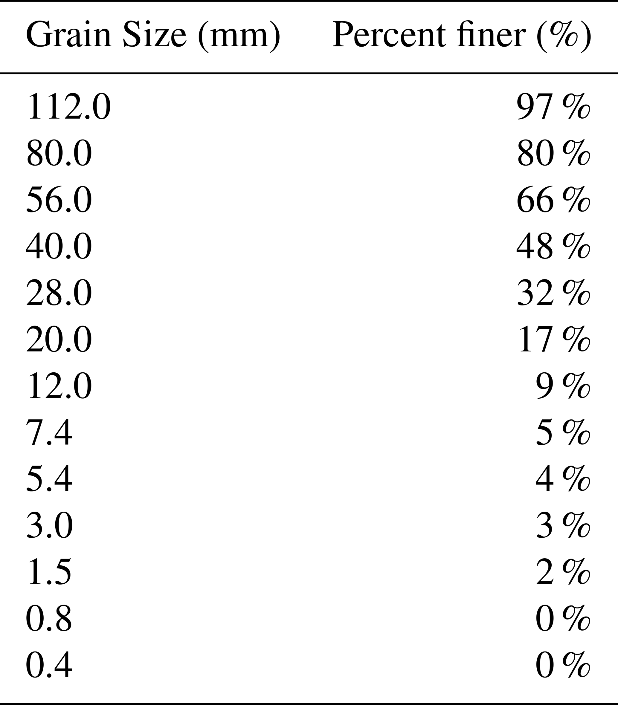
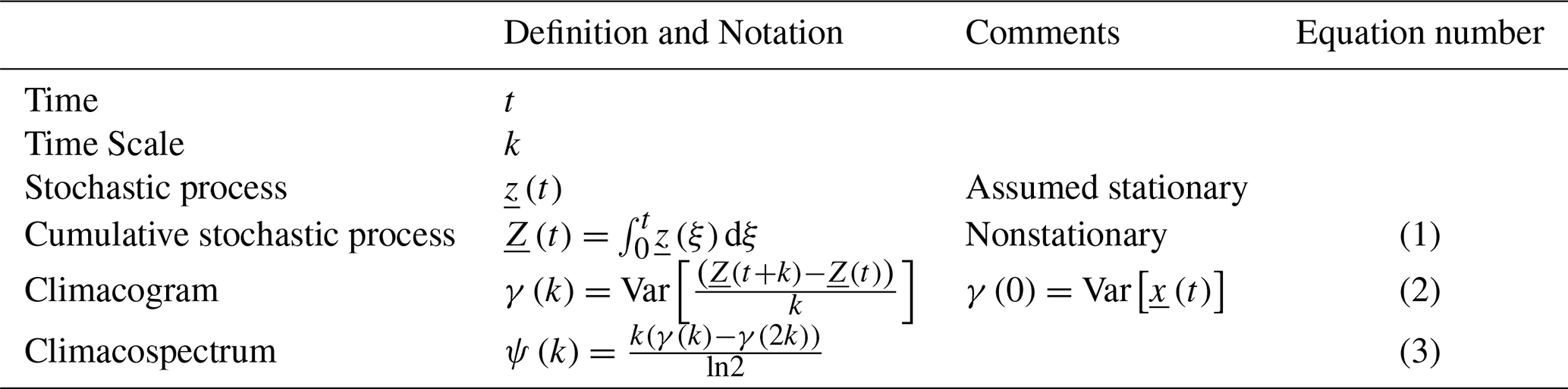
Table 3 Definition of the stochastic tools and notations used for stochastic processes.

2.2 Stochastic streamflow analysis and synthetic time series generation

The dependence structure of the river streamflow process was modelled in terms of the climacogram stochastic tool (see Dimitriadis et al., 2021; Dimitriadis and Koutsoyiannis, 2015; Koutsoyiannis, 2010), defined as the variance γ(k) of the averaged process $\underset{\mathrm{¯}}{z}\left(t\right)$ depending on the averaging time scale k. The climacogram is useful for detecting and evaluating LTP dynamics. For STP and ITP, the climacospectrum stochastic tool is used. Such a stochastic tool was recently introduced by Koutsoyiannis (2016, 2025), having, in most cases, the same asymptotic behaviour and properties as the power spectrum, but is computed only in terms of variances. Consequently, it presents less biased results, making it more convenient for model fitting and identification (Koutsoyiannis, 2016). Table 3 presents the mathematical expressions for the climacogram and climacospectrum stochastic tools

A parsimonious stochastic model was used to fit the dependence structure of the river streamflow process in terms of the climacogram (Filtered Hurst-Kolmogorov model with a generalised Cauchy-Dagum-type climacogram, FHK-CD). The FHK-CD model is general and flexible for any process, regardless of whether the process is rough or smooth, persistent or antipersistent. It has six fitting parameters and can model the dependence structure from small to large temporal scales:

$$\begin{array}{}\text{(4)}& \mathit{\gamma }\left(k\right)={\mathit{\lambda }}_{\mathrm{1}}^{\mathrm{2}}{\left(\mathrm{1}+{\left(k/{\mathit{\alpha }}_{\mathrm{1}}\right)}^{\mathrm{2}}\right)}^{H-\mathrm{1}}+{\mathit{\lambda }}_{\mathrm{2}}^{\mathrm{2}}\left(\mathrm{1}-{\left(\mathrm{1}+{\left(k/{\mathit{\alpha }}_{\mathrm{2}}\right)}^{-\mathrm{2}}\right)}^{-M}\right)\end{array}$$

where λ₁ and λ₂ are scale parameters with dimensions of [x²], α₁ and α₂ are scale parameters with dimensions of [t], and M and H are the fractal and Hurst parameters, respectively. It is worth mentioning that M and H are dimensionless, ranging between 0 and 1, and determine the local and global dependence structure. Eq. (4) can be simplified, when parsimony is sought, by setting ${\mathit{\lambda }}_{\mathrm{1}}={\mathit{\lambda }}_{\mathrm{2}}=\mathit{\lambda }$ and ${\mathit{\alpha }}_{\mathrm{1}}={\mathit{\alpha }}_{\mathrm{2}}=\mathit{\alpha }$. Therefore, the FHK-CD model with four parameters is presented in Eq. (5):

$$\begin{array}{}\text{(5)}& \mathit{\gamma }\left(k\right)={\mathit{\lambda }}^{\mathrm{2}}{\left(\mathrm{1}+{\left(k/\mathit{\alpha }\right)}^{\mathrm{2}}\right)}^{H-\mathrm{1}}+{\mathit{\lambda }}^{\mathrm{2}}\left(\mathrm{1}-{\left(\mathrm{1}+{\left(k/\mathit{\alpha }\right)}^{-\mathrm{2}}\right)}^{-M}\right)\end{array}$$

The variance estimator for the climacogram and climacospectrum can be computed as:

$$\begin{array}{}\text{(6)}& \underset{\mathrm{¯}}{\widehat{\mathit{\gamma }}}\left(k\right)={\displaystyle \frac{\mathrm{1}}{⌊n/\mathit{\kappa }⌋}}\sum _{i=\mathrm{1}}^{⌊n/\mathit{\kappa }⌋}{\left({{\underset{\mathrm{¯}}{z}}_i}^{\left(\mathit{\kappa }\right)}-\underset{\mathrm{¯}}{\widehat{\mathit{\mu }}}\right)}^{\mathrm{2}}\end{array}$$

where $\mathit{\kappa }=k/\mathrm{\Delta }$ is the dimensionless time scale, Δ is the time resolution at each sample time series, $⌊n/\mathit{\kappa }⌋$ is the integer part of $n/\mathit{\kappa }$, and ${{\underset{\mathrm{¯}}{z}}_i}^{\left(\mathit{\kappa }\right)}$ is the ith element of the averaged sample of the process at scale κ, i.e.:

$$\begin{array}{}\text{(7)}& {{\underset{\mathrm{¯}}{z}}_i}^{\left(\mathit{\kappa }\right)}={\displaystyle \frac{\mathrm{1}}{\mathit{\kappa }}}\sum _{j=\left(i-\mathrm{1}\right)\mathit{\kappa }+\mathrm{1}}^{i\mathit{\kappa }}{z}_j\end{array}$$

It is worth mentioning that the bias of variance estimator presented in Eq. (6) can be easily computed by Eq. (8). Additionally, and for fitting purposes, the standardised climacogram ($\underset{\mathrm{¯}}{\widehat{\mathit{\gamma }}}\left(k\right)/\underset{\mathrm{¯}}{\widehat{\mathit{\gamma }}}\left(\mathrm{1}\right)$) and climacospectrum ($\underset{\mathrm{¯}}{\widehat{\mathit{\psi }}}\left(k\right)/\underset{\mathrm{¯}}{\widehat{\mathit{\psi }}}\left(\mathrm{1}\right)$) are used. The effect of the annual cycle was removed following Koutsoyiannis (2019, 2020), i.e. multiplying 12 coefficients (one per month and summing 1 in total) by the streamflow values. The value of the coefficients was found by minimising the variance of the transformed time series.

$$\begin{array}{}\text{(8)}& \mathrm{E}\left[\underset{\mathrm{¯}}{\widehat{\mathit{\gamma }}}\left(k\right)\right]=\mathit{\gamma }\left(k\right)-\mathit{\gamma }\left(⌊n/k⌋k\right)\end{array}$$

For synthetic generation purposes, the asymmetric-moving-average (AMA) scheme is adopted (see Koutsoyiannis, 2019, 2020). The AMA scheme can explicitly preserve any arbitrary second-order dependence structure, as long as a mathematical expression for it exists. The marginal distribution function of the generated data approximates the original one through the statistical moments of the process. In this study, the first four moments are preserved, enabling a good approximation of the original marginal distribution function as was shown in Dimitriadis and Koutsoyiannis (2018). Therefore, the approximation can be carried out with controlled accuracy. The AMA scheme generates ${\underset{\mathrm{¯}}{z}}_i$ by

$$\begin{array}{}\text{(9)}& {\underset{\mathrm{¯}}{z}}_i=\sum _{j=-J}^J{a}_j{\underset{\mathrm{¯}}{v}}_{i-j}\end{array}$$

where a_j are coefficients (weights) computed from the autocovariance function and ${\underset{\mathrm{¯}}{v}}_i$ is white noise. Notice that J is theoretically infinite, although for simulation purposes J is taken as a large integer providing negligible truncation errors (Koutsoyiannis, 2000). A generic solution for a_j was proposed by Koutsoyiannis (2020):

$$\begin{array}{}\text{(10)}& a_j=\underset{-\mathrm{1}/\mathrm{2}}{\overset{\mathrm{1}/\mathrm{2}}{\int }}{e}^{\mathrm{2}\mathit{\pi }\left(\mathit{\theta }\left(\mathit{\omega }\right)-j\mathit{\omega }\right)}{A}^{\mathrm{R}}\left(\mathit{\omega }\right)\mathrm{d}\mathit{\omega }\end{array}$$

where θ(ω) is any real function having the following property $\mathit{\theta }\left(-\mathit{\omega }\right)=-\mathit{\theta }\left(\mathit{\omega }\right)$ and $A^{\mathrm{R}}\left(\mathit{\omega }\right)=\sqrt{\mathrm{2}{s}_d\left(\mathit{\omega }\right)}$. Time asymmetry is handled through the preservation of the skewness ratio between the differenced process ${\underset{\mathrm{¯}}{\stackrel{\mathrm{̃}}{z}}}_{\mathit{\tau }}\left(={\underset{\mathrm{¯}}{z}}_{\mathit{\tau }}-z_{\mathit{\tau }-\mathrm{1}}\right)$ and the original one ${\underset{\mathrm{¯}}{z}}_{\mathit{\tau }}$,

$$\begin{array}{}\text{(11)}& {\displaystyle \frac{{\stackrel{\mathrm{̃}}{C}}_{\mathrm{s}}}{C_{\mathrm{s}}}}={\displaystyle \frac{{\sum }_{j=-J}^J{\left(a_j-a_{j-\mathrm{1}}\right)}^{\mathrm{3}}}{{\left({\sum }_{j=-J}^J{\left(a_j-a_{j-\mathrm{1}}\right)}^{\mathrm{2}}\right)}^{\mathrm{3}/\mathrm{2}}}}{\displaystyle \frac{{\left({\sum }_{j=-J}^J{a}_j^{\mathrm{2}}\right)}^{\mathrm{3}/\mathrm{2}}}{{\sum }_{j=-J}^J{a}_j^{\mathrm{3}}}}\end{array}$$

where ${\stackrel{\mathrm{̃}}{C}}_{\mathrm{s}}$ is the skewness of the differenced process $\underset{\mathrm{¯}}{\stackrel{\mathrm{̃}}{z}}$ and C_s is the skewness of the original process ${\underset{\mathrm{¯}}{z}}_{\mathit{\tau }}$. Note that the skewness ratio depends only on the a_η sequence, and as a consequence, it depends on the (a)symmetric parameter θ(ω). Interesting the fact that θ(ω)=0 implies time symmetry and AMA converges to the symmetric moving average (SMA) scheme. However, $\mathrm{0}<\mathit{\theta }\left(\mathit{\omega }\right)\le \mathrm{1}/\mathrm{4}$ preserves time asymmetry. As a consequence, θ(ω) must be chosen to preserve the skewness ratio. It is worth mentioning that time asymmetry is an important feature of streamflow at time scales up to four days (see Koutsoyiannis, 2019; Vavoulogiannis et al., 2021) and consequently, it should be preserved when working at the hourly scale. Figure 2 shows an example of synthetically generated streamflow using AMA with two different θ values. Notice that θ=0.00 generates symmetric-to-the-peak time series, whereas θ=0.10 generates positively asymmetric time series.

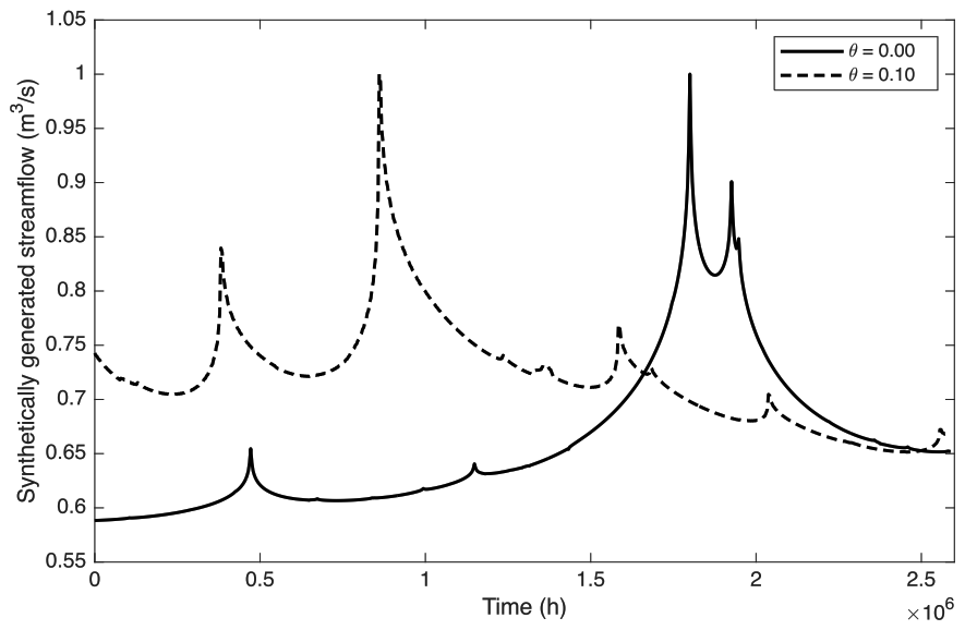
Figure 2 Example of synthetically generated streamflow using AMA with two different θ values. Notice that θ=0.00 generates symmetric-to-the-peak time series, whereas θ=0.10 generates positively asymmetric time series. Generator setup: M=0.54; H=0.64; α=486 h; mean, variance, skewness, and kurtosis were 30 m³ s⁻¹, 10 m⁶ s⁻², 10, 4, respectively. Plotted Q is the standardised synthetically generated streamflow, i.e. $Q/\max \left(Q\right)$.

2.3 Computation of time-dependent local scour and fill at a bridge pier

The bridge-pier scour entropic (BRISENT) model is considered for time-dependent scour analysis because of its flexibility and parsimonious modelling within time-dependent hydraulic conditions (Pizarro et al., 2017a). BRISENT relies on the principle of maximum entropy and on the effective flow work parameter, W^* (Pizarro et al., 2017b), which accounts for the influence of flood waves on the local scour process. W^* is mathematically defined as follows:

$$\begin{array}{}\text{(12)}& W^{*}\left(t_{\mathrm{con}}\right)=\underset{\mathrm{0}}{\overset{t_{\mathrm{con}}}{\int }}{\displaystyle \frac{\mathrm{1}}{t_{\mathrm{R}}}}{\left({\displaystyle \frac{u\left(t\right)-\mathrm{0.5}{u}_{\mathrm{c}}}{u_{\mathrm{R}}}}\right)}^{\mathrm{4}}\mathit{\delta }\mathrm{d}t\end{array}$$

where t_con is the considered time, t_R is a reference time defined as $z_{\mathrm{R}}/u_{\mathrm{R}}$, $z_{\mathrm{R}}=D^{\mathrm{2}}/\mathrm{2}{d}_{\mathrm{50}}$ is a reference length (D is the pier-diameter and d₅₀ the sediment-size), u(t) is the time-dependent section averaged flow velocity, u_R is a reference velocity ($=\sqrt{\mathit{\rho }{}^{\prime }g{d}_{\mathrm{50}}}$, where $\mathit{\rho }{}^{\prime }=\left({\mathit{\rho }}_{\mathrm{S}}-{\mathit{\rho }}_{\mathrm{W}}\right)/{\mathit{\rho }}_{\mathrm{W}}$ is the relative density between sediment “s” and water “w”, and g is the gravitational acceleration). u_c is the critical flow velocity for incipient motion of sediment particles and δ is an on-off step function defined as:

$$\begin{array}{}\text{(13)}& \mathit{\delta }=\left\{\begin{array}{ll}\mathrm{0},& u\left(t\right)/u_{\mathrm{c}}<\mathrm{0.5}\\ \mathrm{1},& u\left(t\right)/u_{\mathrm{c}}\ge \mathrm{0.5}\end{array}\right.\end{array}$$

The BRISENT model has three model parameters ($\mathit{\lambda },W_{\max }^{*}$, and S) and their empirical expressions rely on a large laboratory dataset with a wide range of key dimensionless parameters which control the scour process. BRISENT is presented in Eq. (14), while from Eq. (15) to (17) are the empirical expressions for the fitting parameters.

$$\begin{array}{}\text{(14)}& {\displaystyle }{Z}^{*}={\displaystyle \frac{\mathrm{1}}{\mathit{\lambda }}}\ln \left\{\mathrm{1}+{\displaystyle \frac{W^{*}}{W_{\max }^{*}}}\left[\exp \left(S\right)-\mathrm{1}\right]\right\}\text{(15)}& {\displaystyle }\mathit{\lambda }=\mathrm{4.237}{\left({\displaystyle \frac{D}{d_{\mathrm{50}}}}\right)}^{\mathrm{0.957}}\text{(16)}& {\displaystyle }{W}_{\max }^{*}=\exp \left[\mathrm{21.84}{\left(\ln {\displaystyle \frac{D}{d_{\mathrm{50}}}}\right)}^{-\mathrm{0.295}}\right]\text{(17)}& {\displaystyle }S={\displaystyle \frac{\mathrm{21.185}{\left(D/d_{\mathrm{50}}\right)}^{\mathrm{0.957}}}{\mathrm{0.4}{\left(D/d_{\mathrm{50}}\right)}^{\mathrm{1.2}}+\mathrm{10.6}{\left(D/d_{\mathrm{50}}\right)}^{-\mathrm{0.13}}}}.\end{array}$$

The three parameters defining the BRISENT response have distinct physical and statistical roles. The dimensionless effective flow work, W^*, represents the cumulative hydraulic forcing the flow applies on the sediment bed around the pier. It incorporates both the magnitude and duration of the flow. Its limiting value, $W_{\max }^{*}$, represents the cumulative effective flow work associated with the maximum relative scour depth $Z_{\max }^{*}$, ideally corresponding to equilibrium scour. It normalises the process between its initial and final states. The dimensionless parameter λ originates as a Lagrange multiplier in the maximum-entropy derivation and controls the exponential form of the relative-scour probability distribution and, consequently, the curvature of the scour-work relationship. Finally, S is the dimensionless entropic-scour parameter linking λ to the maximum relative scour depth. It controls the degree of non-linearity in the response, with larger values indicating more rapid initial scour development followed by progressively slower development to its maximum value.

The scour hole refilling process was considered, following Link et al. (2020), i.e., sediment deposition occurring during the falling limb of the hydrograph. The time-dependent sediment deposition rate, d(t), was computed as

$$\begin{array}{}\text{(18)}& d\left(t\right)={\mathit{\alpha }}_{\mathrm{d}}{\displaystyle \frac{w_{\mathrm{s}}}{q\left(t\right)}}\left(g_{\mathrm{s}}\left(t\right)-g_{\mathrm{s}}^{*}\left(t\right)\right)\end{array}$$

where, α_d is considered a constant (=0.5 according to Link et al., 2020; Pizarro et al., 2022a), w_s is the sediment falling velocity, q(t) is the specific discharge per unit width, g_s(t) is the sediment supply rate (kg m s⁻¹), and $g_{\mathrm{s}}^{*}\left(t\right)$ is the sediment transport capacity (kg m s⁻¹) estimated using the Meyer-Peter and Müller (1948) equation:

$$\begin{array}{}\text{(19)}& g_{\mathrm{s}}^{*}=\mathrm{8}{\mathit{\rho }}_{\mathrm{s}}{\left(\mathit{\rho }{}^{\prime }g{d}_{\mathrm{s}}^{\mathrm{3}}\right)}^{\mathrm{0.5}}{\left[{\left({\displaystyle \frac{C_{\mathrm{R}}}{C_{\mathrm{R}}{}^{\prime }}}\right)}^{\mathrm{1.5}}\mathrm{\Theta }-{\mathrm{\Theta }}_c\right]}^{\mathrm{1.5}}\end{array}$$

where C_R is the total Chézy coefficient due to effective bed roughness k_s ($=\mathrm{18}\log \left(\mathrm{12}h/k_{\mathrm{s}}\right)$), C_R^′ is the Chézy coefficient due to particle roughness d₉₀ ($=\mathrm{18}\log \left(\mathrm{12}h/d_{\mathrm{90}}\right)$), and Θ and Θ_c are the Shields and threshold Shields parameters.

The presented deposition modelling framework considers sediment deposition if the hydrograph is in the falling limb and $g_{\mathrm{s}}\left(t\right)>g_{\mathrm{s}}^{*}\left(t\right)$. g_s(t) is estimated as $g_{\mathrm{s}}^{*}\left(t\right)$ evaluated in the previous instant, i.e. $g_{\mathrm{s}\left[i\right]}=\mathit{\xi }{g_{\mathrm{s}}^{*}}_{\left[i-\mathrm{1}\right]}$, where ξ is an exceedance sediment supply coefficient and i reports the discrete time instant. In consequence, the sediment deposition depth is calculated through a fractional transport formulation as follows:

$$\begin{array}{}\text{(20)}& d_{\left[i\right]}={\displaystyle \frac{{\mathit{\alpha }}_{\mathrm{d}}}{{\mathit{\rho }}_{\mathrm{s}}\left(\mathrm{1}-p\right)}}\sum _{j=\mathrm{1}}^n{\displaystyle \frac{w_{{\mathrm{s}}_{\left[j\right]}}{P}_{\left[j\right]}}{q_{\left[i\right]}}}\left(\mathit{\xi }{g_{\mathrm{s}}^{*}}_{\left[i-\mathrm{1},j\right]}-{g_{\mathrm{s}}^{*}}_{\left[i,j\right]}\right)\mathrm{\Delta }t\end{array}$$

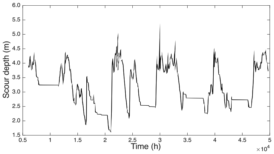
where j is a counter for the considered sediment sizes in the granulometric curve, ρ_s is the sediment density, p is the sediment porosity, and P_[j] is the percentage of the soil which contains the sediment size d_s[j]. Therefore, the scour depth considering the refilling scour process is computed as $z_{\left[i\right]}=z_{{\mathrm{scour}}_{\left[i\right]}}-d_{\left[i\right]}$ and $W_{\left[i\right]}^{*}=W_{{\mathrm{scour}}_{\left[i\right]}}^{*}-\mathrm{\Delta }{\mathrm{W}}_{d_{\left[i\right]}}^{*}$. The scour and deposition models were implemented in a software package, and a sensitivity analysis of their parameters was presented by Pizarro et al. (2022a). Figure 3 shows an example of scour depth time series computed with the scour and fill models. It is worth mentioning that erosional and sediment (re)deposition dynamics are captured by the simulation.

Figure 3 Example of scour depth time series using the scour and fill model.

Equilibrium scour (z_eq) is computed with the widely used scour equation by Sheppard et al. (2014):

$$\begin{array}{}\text{(21)}& {\displaystyle \frac{z_{\mathrm{eq}}}{a^{*}}}=\mathrm{2.5}{f}_{\mathrm{1}}{f}_{\mathrm{2}}{f}_{\mathrm{3}}\mathrm{for}\mathrm{0.4}\le {\displaystyle \frac{u}{u_{\mathrm{c}}}}<\mathrm{1.0}\text{(22)}& {\displaystyle }\begin{array}{rl}{\displaystyle \frac{z_{\mathrm{eq}}}{a^{*}}}& =f_{\mathrm{1}}\left[\mathrm{2.2}\left({\displaystyle \frac{\frac{u}{u_{\mathrm{c}}}-\mathrm{1}}{\frac{u_{\mathrm{1}\mathrm{p}}}{u_{\mathrm{c}}}-\mathrm{1}}}\right)+\mathrm{2.5}{f}_{\mathrm{3}}\left({\displaystyle \frac{\frac{u_{\mathrm{1}\mathrm{p}}-u}{u_{\mathrm{c}}}}{\frac{u_{\mathrm{1}\mathrm{p}}}{u_{\mathrm{c}}}-\mathrm{1}}}\right)\right]\\ & \mathrm{for}\mathrm{1.0}<{\displaystyle \frac{u}{u_{\mathrm{c}}}}<{\displaystyle \frac{u_{\mathrm{1}\mathrm{p}}}{u_{\mathrm{c}}}}\end{array}\text{(23)}& {\displaystyle \frac{z_{\mathrm{eq}}}{a^{*}}}=\mathrm{2.2}{f}_{\mathrm{1}}\mathrm{for}{\displaystyle \frac{u}{u_{\mathrm{c}}}}>{\displaystyle \frac{u_{\mathrm{1}\mathrm{p}}}{u_{\mathrm{c}}}}\text{(24)}& {\displaystyle }{u}_{\mathrm{1}\mathrm{p}\mathrm{1}}=\mathrm{5}{u}_{\mathrm{c}}\text{(25)}& {\displaystyle }{u}_{\mathrm{1}\mathrm{p}\mathrm{2}}=\mathrm{0.6}\sqrt{g{y}_{\mathrm{1}}}\text{(26)}& {\displaystyle }{u}_{\mathrm{1}\mathrm{p}}=\left\{\begin{array}{l}{u}_{\mathrm{1}\mathrm{p}\mathrm{1}}\mathrm{for}{u}_{\mathrm{1}\mathrm{p}\mathrm{1}}\ge u_{\mathrm{1}\mathrm{p}\mathrm{2}}\\ u_{\mathrm{1}\mathrm{p}\mathrm{2}}\mathrm{for}{u}_{\mathrm{1}\mathrm{p}\mathrm{1}}<u_{\mathrm{1}\mathrm{p}\mathrm{2}}\end{array}\right.\text{(27)}& {\displaystyle }{f}_{\mathrm{1}}=\tanh \left[{\left({\displaystyle \frac{h}{a^{*}}}\right)}^{\mathrm{0.4}}\right]\text{(28)}& {\displaystyle }{f}_{\mathrm{2}}=\left\{\mathrm{1}-\mathrm{1.2}{\left[\ln \left({\displaystyle \frac{u}{u_c}}\right)\right]}^{\mathrm{2}}\right\}\text{(29)}& {\displaystyle }{f}_{\mathrm{3}}=\left[{\displaystyle \frac{\left(\frac{a^{*}}{d_{\mathrm{50}}}\right)}{\mathrm{0.4}{\left(\frac{a^{*}}{d_{\mathrm{50}}}\right)}^{\mathrm{1.2}}+\mathrm{10.6}{\left(\frac{a^{*}}{d_{\mathrm{50}}}\right)}^{-\mathrm{0.13}}}}\right]\end{array}$$

2.4 Extreme events detection and return periods

To assess the correspondence between the detection of extreme events in streamflow and scour, the critical success index (CSI, see Eq. 30) was used. The CSI computed the number of hits (H), misses (M) and false alarm (F) events. Hits are defined as matching events identified for both streamflow and scour, whereas misses are events identified only for streamflow. False alarm events are those identified only for scour. CSI ranges between 0 and 1, with the latter the optimum value. We defined hits as the scour events that overlap with the streamflow events by at least 70 %. A tolerance of 2 h before and 2 h after the original event identification was considered, accounting for possible uncertainty in the event identification procedure. The threshold for streamflow and scour events identification was the 40th percentile of the annual maxima series.

$$\begin{array}{}\text{(30)}& \mathrm{CSI}={\displaystyle \frac{H}{H+M+F}}\end{array}$$

Return periods of scour depths were computed directly from the scour time series using annual maxima series and fitting the Generalised Extreme Value (GEV) probability distribution function. A low CSI indicates poor temporal correspondence between detected streamflow and scour events, but it could not by itself demonstrate that conventional streamflow-based design produces biased scour return levels.

2.5 Monte Carlo simulations

Monte Carlo analysis was performed with N=12 000 simulations, each of them with 60 years at an hourly temporal scale of the synthetic generated streamflow time series. These simulations were used as input for the time-dependent scour and fill model, generating the same number of scour time series. Additionally, and with the intention to assess the effect of upstream sediment supply on scour (and, therefore, the sediment deposition effect), three different cases were investigated: (i) ξ=1.0; (ii) ξ=1.5; and, (iii) ξ=2.0. The latter cases range from sediment rates equal to the transport capacity (i.e., ξ=1.0) to sediment supply exceeding the transport capacity (i.e., ξ=1.5 and ξ=2.0). In total, 36 000 simulations (12 000 for each ξ case) were performed.

2.6 Methodology outline summary

The methodology employed in this work encompasses the stochastic analysis of the Trancura River gauging station and the synthetic generation of river streamflow time series, which preserves time asymmetry, the second-order dependence structure, and the probability density function (through the first four statistical moments). Synthetic streamflow time series were replicates of the historical record and the inputs for the time-dependent scour and fill model. Monte Carlo analysis was performed with N=12 000 simulations, each of them with 60 years at an hourly temporal scale of the synthetic generated streamflow time series and scour time series. Three different cases of upstream sediment supply having a sediment rate equal to the transport capacity (i.e., ξ=1.0) and sediment supply 50 % and 100 % higher than the transport capacity (i.e., ξ=1.5 and ξ=2.0, respectively). The stochastic properties of the scouring process were quantified in terms of the second-order dependence structure, the Hurst and Mandelbrot parameters, and time asymmetry through the skewness of the differenced process. The non-stochastic properties of the scouring process were quantified in terms of the CSI index and scour return periods following Rifo et al. (2022).

2.7 Code availability

Codes for streamflow generation and scour computation were written in MATLAB and are available at Pizarro et al. (2025). In particular, the scripts consider the analysis and modelling of the river streamflow process, its synthetic generation (using the AMA scheme, which preserves time asymmetry, the second-order stochastic properties, and the first four statistical moments), and the scour assessment following the methodology described above.

3 Results

3.1 Synthetic-generated streamflow coupled with scour and fill model

Figure 4 shows a representative example of the synthetically generated hourly streamflow series (orange) and the corresponding scour-depth response (blue) over a 60-year simulation period (one of the 36 000 simulations performed). As shown in Fig. 4, the simulated streamflow time series exhibits pronounced variability, with recurrent peaks associated with high-flow events and recessions during lower-flow periods. These dynamics are consistent with the hydrological behaviour of the catchment. In this specific realisation, the maximum and median streamflow values reached 2299 and 94 m³ s⁻¹, respectively, reflecting both the extreme events and the central tendency captured by the stochastic generator.

The blue curve shows the evolution of scour depth, computed by coupling the AMA-generated streamflow with the erosional and fill model under the assumption of ξ=1.0 (i.e., sediment supply equal to the transport capacity). The resulting scour-depth fluctuations showed deeper scour during high-magnitude streamflow peaks. Maximum and median scour depths for this simulation were 5.63 and 3.29 m, demonstrating the model's capacity to translate hydrological variability into adjustments in sediment dynamics. Overall, Fig. 4 highlights the value of integrating stochastic flow generation with process-based scour modelling, enabling the exploration of long-term scour response under a wide ensemble of hydrological conditions.

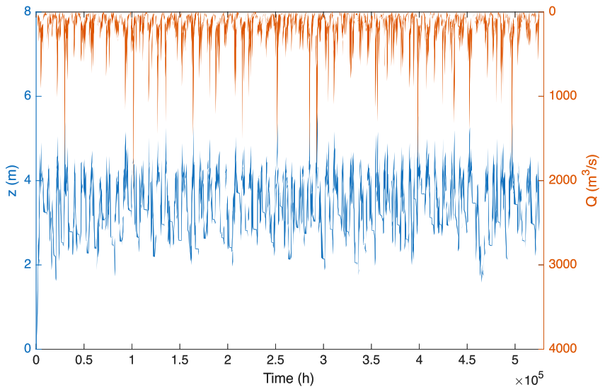
Figure 4 Synthetically generated hourly streamflow and corresponding scour depth over 60 years, considering ξ=1.0 (i.e., sediment rate equal to the transport capacity).

3.2 Deterministic properties of the scouring process

Deterministic properties of the scour process were assessed through the Critical Success Index (CSI) – between river streamflow and bridge scour – and the ratio between the magnitude of scour with a particular return period (computed from the scour simulations) and the equilibrium scour depth computed with the scour formula by Sheppard et al. (2014). Figure 5 shows that the three analysed cases (colours blue, red, and yellow are related to ξ values of 1.0, 1.5, and 2.0, respectively) yielded similar CSI values, ranging from approximately 0.15 to 0.60. A value of 0.15 means that only 15 % of all identified events occurred simultaneously for both river streamflow and scour. A trend from symmetric to positively asymmetric distribution of CSI's values for ξ equal 1.0 to 2.0 (CSI median values are 0.33, 0.32, and 0.30 for ξ equal 1.0, 1.5, and 2.0, respectively) is observed. The resulting low CSI values indicate poor temporal correspondence between detected streamflow and scour events. However, this does not necessarily imply that streamflow-based design produces biased scour return levels.

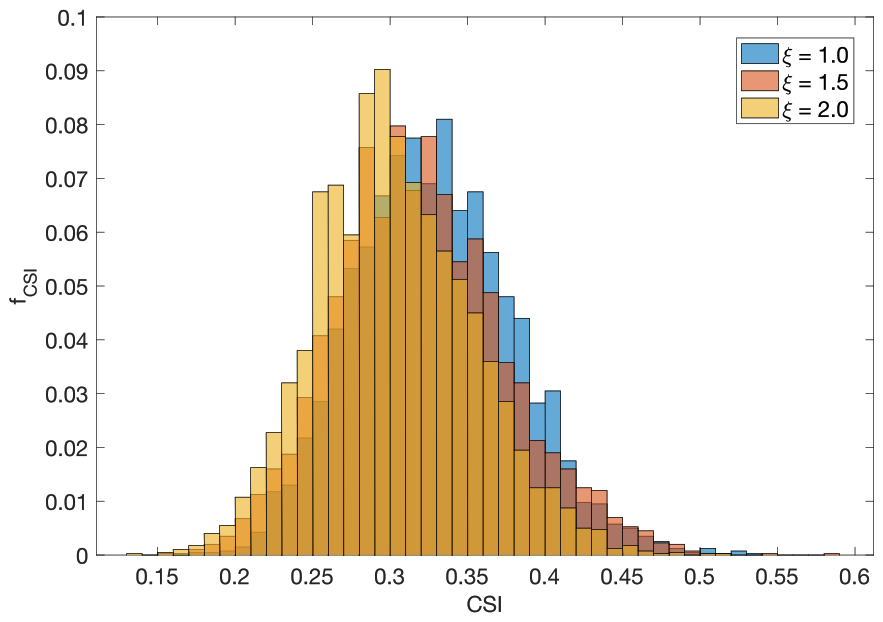
Figure 5 Histograms for the Critical Success Index (CSI) between river streamflow and bridge scour. Blue, red, and yellow colours are related to ξ equals to 1.0, 1.5, and 2.0.

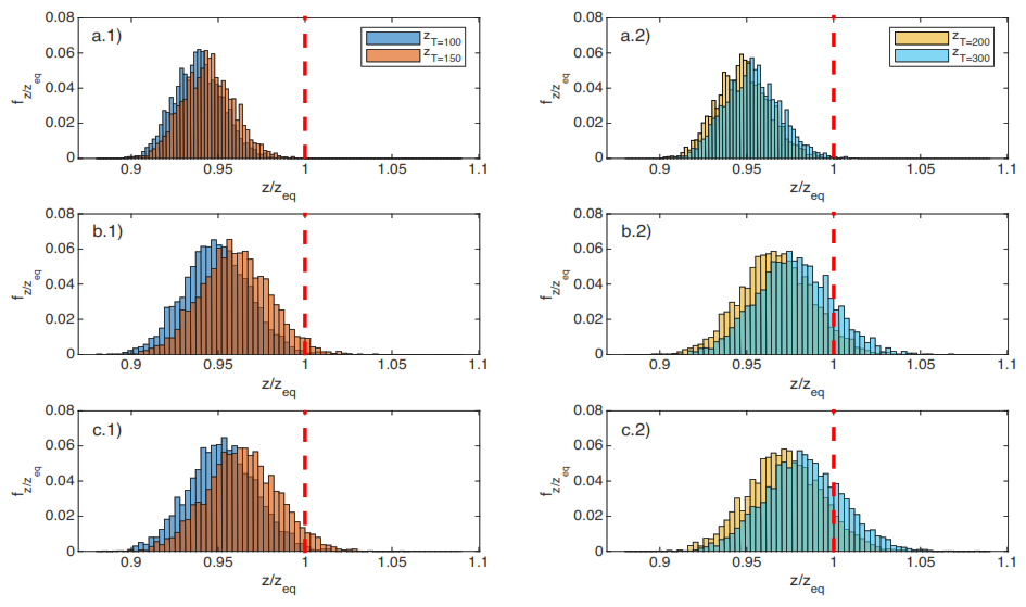
Figure 6 Scour depth to equilibrium scour depth ratio for different return periods and upstream sediment supply with ξ=1.0 (a), 1.5 (b), and 2.0 (c). The red vertical dash lines are explicitly plotted at $z/z_{\mathrm{eq}}=\mathrm{1}$.

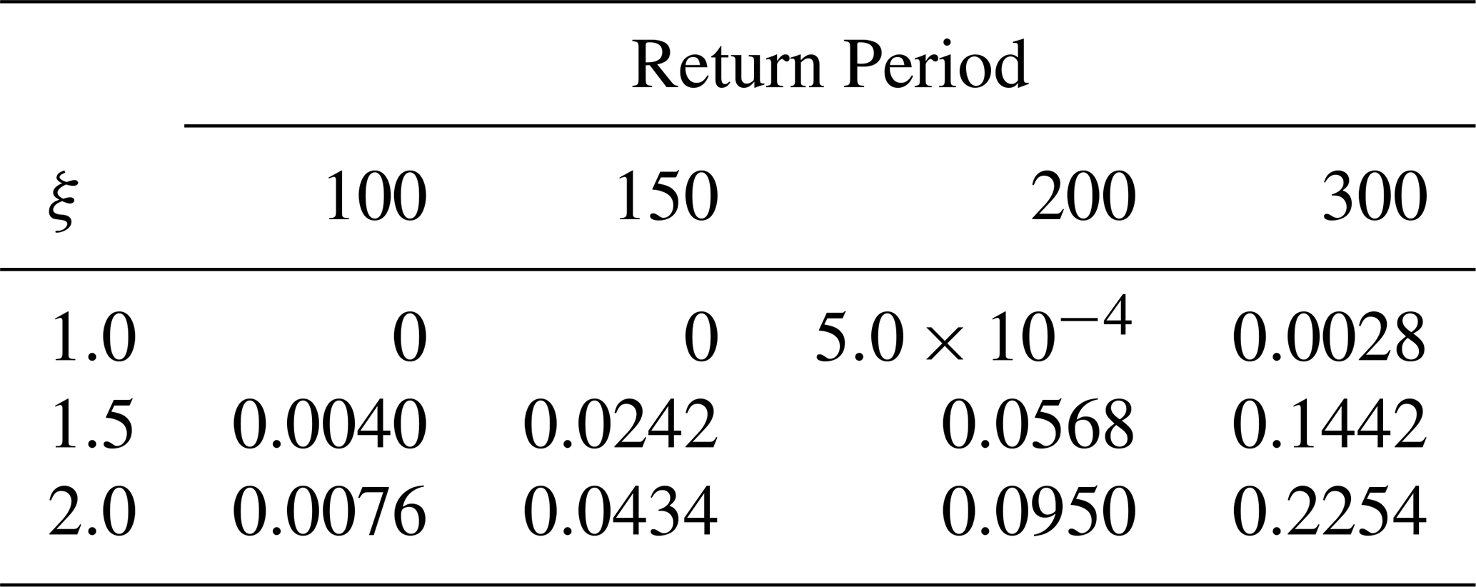
Figure 6 shows the frequency distribution of the computed scour depth with T=100 (blue), 150 (orange), 200 (yellow), and 300 (cyan) years for each scenario of upstream sediment supply with ξ=1.0, 1.5, and 2.0. The above-mentioned return periods were selected due to their direct relationship with risk levels and design methods. Notice that z_eq was computed with the equilibrium scour equation by Sheppard et al. (2014) (i.e., from Eq. 21 to 29) and assuming hydraulic variables associated with a 100-year flood event. Therefore, if $z_{T=\mathrm{100}}=z_{\mathrm{eq}}$(i.e., the median of scour depths with T=100 years computed from scour time series is equal to the equilibrium scour depth), the same return period will be related to both processes. In all cases, the scour depth to equilibrium scour depth ratio ($z/z_{\mathrm{eq}}$) increased with ξ. In most analysed cases, scour depths computed with scour time series were different and higher than the equilibrium scour depth (especially for T=200 and T=300 years). As a consequence, and considering that the median for $z_{T=\mathrm{100}}/z_{\mathrm{eq}}$ is between 0.93 and 0.95 (for all analysed ξ), a given return period of streamflow does not necessarily translate into the same return period of scour. Exceedance probabilities for $z_{T=\mathrm{100}}/z_{\mathrm{eq}}$ were lower than 0.0076 for all analysed cases. Table 4 shows the exceedance probability for $z/z_{\mathrm{eq}}>\mathrm{1.0}$.

Table 4 Exceedance probability for $z/z_{\mathrm{eq}}>\mathrm{1.0}$ as a function of the considered return period and upstream sediment supply.

3.3 Stochastic properties of the scouring process

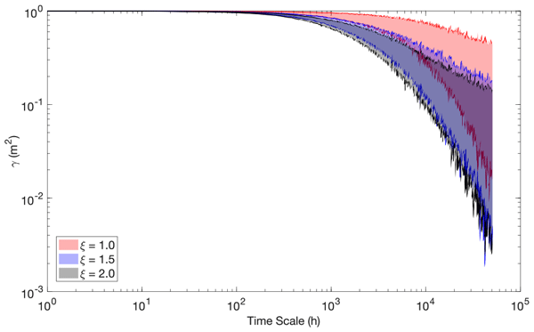
The second-order dependence structure was quantified in terms of the climacogram and climacospectrum adapted for bias. All computations were standardised by dividing them by their first value. Only 90 % of all available scales were used for model fitting purposes, mainly motivated by the high calculation uncertainty in small samples (i.e., with less than 10 values. See Dimitriadis and Koutsoyiannis, 2015). Figure 7 shows the envelope standardised climacograms as a function of ξ=1.0 (red), 1.5 (blue), and 2.0 (black). It is worth noticing that the higher the ξ value, the narrower the envelopes; and, climacograms for ξ=1.5 and ξ=2.0 are similar.

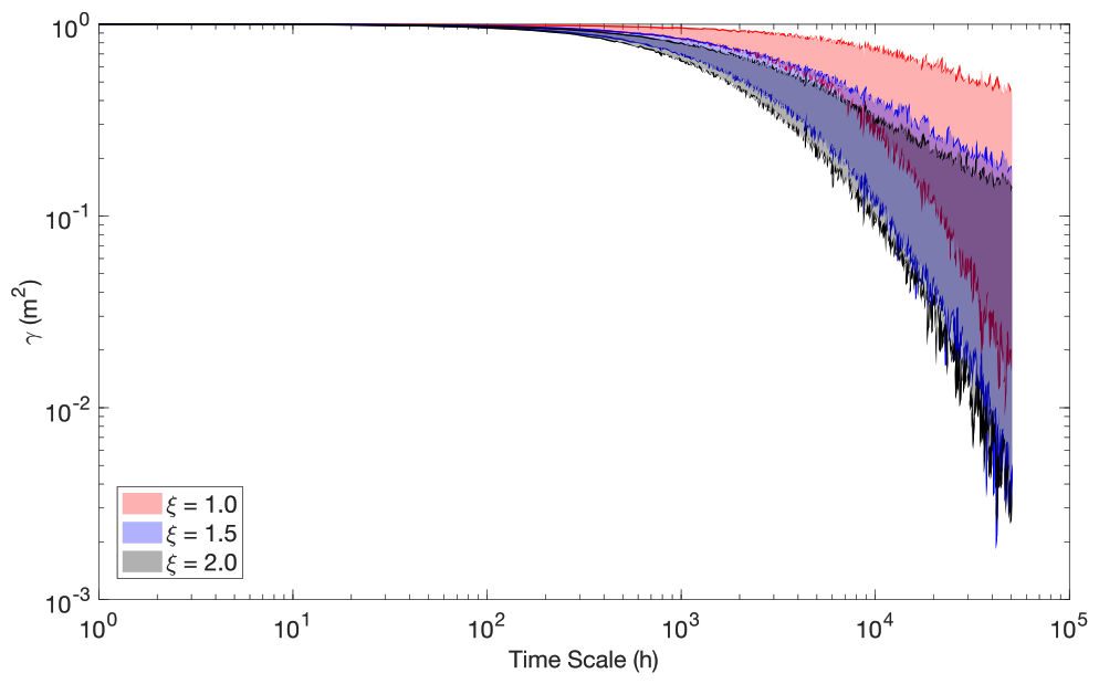
Figure 7 Envelope standardised climacograms for ξ equals to 1.0 (red), 1.5 (blue), and 2.0 (black). Each envelope takes into consideration 12 000 scour simulations.

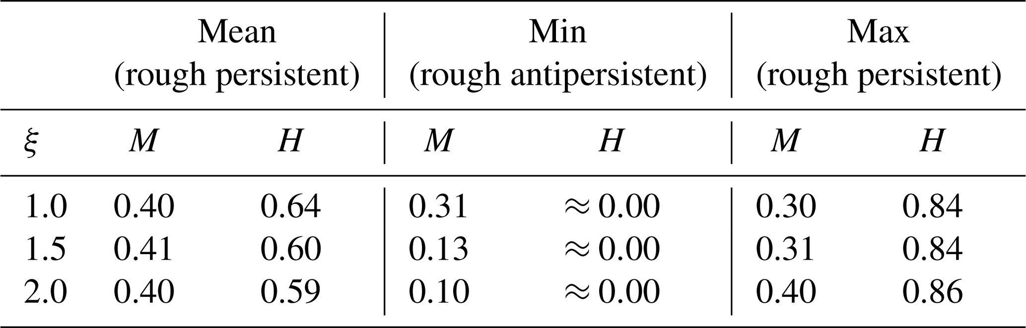
Figure 8 shows the mean standardised climacograms and climacospectrums for ξ equals to 1.0 (red), 1.5 (blue), and 2.0 (black). Mean standardised stochastic tools were considered as representative of the 12 000 simulations. The continuous green line corresponds to the FHK-CD model. Interestingly, asymptotic dynamics at both small (assessed through the Mandelbrot parameter, M) and large (assessed through the Hurst parameter, H) temporal scales yielded similar values (M≈0.40 and H≈0.60). The latter is indicative of rough and (weak) persistent dynamics. Table 5 summarises these asymptotic behaviours for the means and envelopes. Mean values are related to the mean standardised stochastic tool, while min and max correspond to the lower and upper envelopes.

Interestingly, and focusing on the envelopes, the strength of the Hurst dynamics of the scouring process depends on ξ, ranging from H≈0.00 (strong antipersistence dynamics) to H=0.86 (strong LTP dynamics). On the other hand, the Mandelbrot parameter took values from 0.10 to 0.41 (i.e., having less variability than H). It is worth mentioning that rough dynamics (i.e., M<0.5) instead of a smooth one (i.e., M>0.5) is usual in many hydrological processes at the analysed hourly scale such as the cases of near-surface temperature, relative humidity, dew point, sea level pressure, wind speed, and precipitation (see, e.g., Dimitriadis and Koutsoyiannis, 2018; Pizarro et al., 2022b).

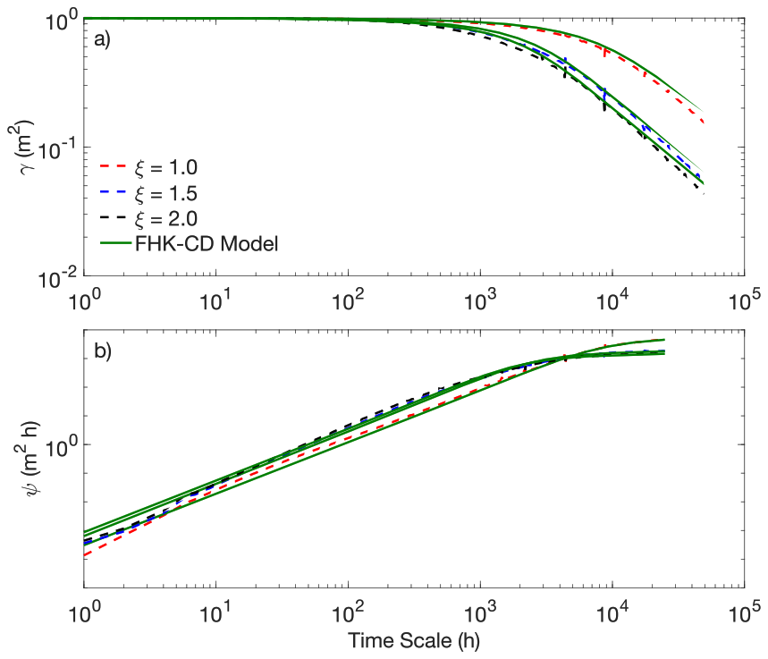
Figure 8 Mean standardised climacograms and climacospectrum for ξ equals to 1.0 (red), 1.5 (blue), and 2.0 (black). The continuous green line is the FHK-CD model.

Table 5 Summary of asymptotic behaviours at small (M, Mandelbrot or fractal parameter) and large (H, Hurst parameter) scales. Mean values are related to the mean standardised stochastic tool, while min and max correspond to the envelopes. The minimum temporal scale under analysis was hourly.

In terms of time asymmetry, the scour process showed negative skewness coefficients at short time scales, followed by a transition to positive values and convergence towards zero at longer time scales (see Fig. 9). This behaviour indicates that scour increments are not time-symmetric: large negative fluctuations dominate at fine resolutions, while positive dynamics emerge as aggregation increases. A systematic dependence of the scour depth on ξ, i.e. on the upstream sediment supply, was observed. For ξ=1.0, 1.5, and 2.0, the transition from negative to positive skewness occurred at approximately 195 (h), 80 (h), and 54 (h), respectively. The subsequent return from positive to near-zero values occurred at around 20 000 (h), 6500 (h), and 5000 (h) for the same ξ values. These thresholds reveal that higher sediment availability reduces the persistence of asymmetry, leading to faster stabilisation of scour fluctuations.

The observed scale-dependent dynamics confirm that bridge scour cannot be described solely by equilibrium formulations, which ignore time asymmetry and stochastic persistence. Instead, our findings highlighted that skewness provides an additional diagnostic tool to assess the temporal structure of scour variability, especially in the presence of fill in the scour hole due to upstream sediment supply. Incorporating time asymmetry into stochastic frameworks, therefore, enhances the reliability of probabilistic scour hazard assessments.

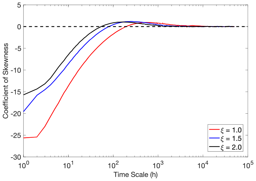
Figure 9 Skewness coefficient of the differenced scour time series as a function of the time scale. Plots refer to the standardised series, which take the mean value of the 12 000 simulations. ξ equals to 1.0, 1.5, and 2.0 are related to the colours red, blue, and black; respectively.

4 Strengths and limitations

A key strength of this work is the physically consistent coupling between a parsimonious stochastic streamflow generator (AMA) – that preserves the HK dynamics, the second-order dependence structure, time asymmetry, and the first four statistical moments of the marginal distribution – and time-dependent scour and fill models that includes both erosional and sediment (re)deposition dynamics. The latter framework enables the synthetic generation of more realistic scour time-series during the entire bridge lifespan, capturing complex hydrological dynamics and their associated behaviour in terms of erosion and fill of sediments (that equilibrium formulas cannot account for). The framework is representative at multiple temporal scales: the joint use of climacogram and climacospectrum (with bias correction) quantifies roughness (M) and persistence (H), allowing for a rigorous examination of short-, intermediate- and long-term dependence and their implications for forensic scour analysis. Methodologically, the study considers a long, hourly, near-natural record from Southern Chile, thereby improving the computation of the effective flow work and the fidelity of possible hydrological dynamics. Uncertainty was explored in a structured way: >12 000 Monte Carlo realisations across three sediment-supply scenarios (ξ) yield envelope and mean behaviours, explicitly separating sediment fill effects. Additionally, the extreme-value analysis compares scour dynamics with the equilibrium scour depth, directly informing risk-based design (e.g., exceedance probabilities of $z/z_{\mathrm{eq}}>\mathrm{1}$) rather than relying on single deterministic values. Finally, transparent reproducibility (MATLAB code availability) facilitates transfer to other sites and contexts.

In terms of limitations, the hourly resolution does not resolve sub-hourly intermittency or turbulence linked to the initiation/instability of scour holes. The latter might affect the timing and peak of scour events in flash floods. On the case study side, the bridge and reach representation is simplified (single cylindrical pier, 1D approach), excluding contraction scour, debris/ice impacts, sediment armouring, complex bedforms, and explicit 3D flow-structure interactions. In terms of scour model formulations, α_d and ξ (fill model parameters) are treated with constant values that do not change on time. Long field time series of scour depth at bridges are scarce; consequently, findings' validation relies on the plausibility of hydraulics and physics, as well as comparative metrics (e.g., CSI), rather than continuous observed scour time series. Finally, site specificity (Trancura catchment hydrology) limits immediate generalisation to other hydroclimates and sediment regimes without further analysis.

5 Conclusions

This study introduced a novel framework to investigate the stochastic and non-stochastic properties of the bridge scour process by coupling a parsimonious stochastic streamflow generator with a time-dependent scour model that accounts for both erosion and sediment fill. The stochastic generator, based on the asymmetric moving average (AMA) scheme, preserves the Hurst-Kolmogorov dynamics, the second-order dependence structure, time asymmetry, and the first four statistical moments of streamflow. The time-dependent scour model (BRISENT with sediment fill extensions) allowed the simulation of realistic scour depth time series under synthetic hydrographs. Monte Carlo experiments using 12 000 realisations across multiple sediment-supply scenarios produced a rich dataset for characterising scour variability, persistence properties, and exceedance probabilities. The main findings of the study can be summarised as follows:

• Scour is inherently stochastic: The generated scour time series showed persistence across short, intermediate, and long temporal scales, with Hurst parameters reaching values as high as 0.86 under certain sediment-supply scenarios. This reinforces that scour dynamics cannot be adequately represented by equilibrium formulas alone.

• Upstream sediment supply significantly alters scour statistics: Including upstream sediment supply and sediment fill dynamics reduced variability in envelopes and altered both the persistence structure and extreme-value behaviour. Neglecting redeposition leads to an overestimation of long-term scour growth and design depths.

• Equilibrium scour depth is not a reliable upper bound: Comparisons between scour simulations and equilibrium scour estimates demonstrated that the ratio $z/z_{\mathrm{eq}}$ frequently exceeded unity, especially for higher return periods and elevated sediment-supply scenarios. These findings question the common practice of relying on equilibrium scour depth as a conservative design envelope.

• Scour–streamflow synchronisation is weak: The Critical Success Index (CSI) values between streamflow and scour extreme events ranged between 0.15 and 0.60, with mean values around 0.30 to 0.35, showing that not all hydrological extremes translate directly into scour extremes, and thus the time-dependent scour computation caused by long hydrographs is important in scour analysis.

• Return period interpretation is challenged under persistence: The presence of long-term persistence implies higher uncertainty in design scour estimates, reducing the validity of classical return period concepts. Stochastic risk-based design approaches are needed.

Future research directions should focus on extending and generalising the proposed framework. First, further work is needed to validate scour simulations against long-term field observations, particularly from surveys at bridge sites. Second, incorporating more complex pier geometries, contraction scour, debris and ice effects, and armouring processes would improve the realism of simulations. Third, uncertainty quantification should be advanced by adopting Bayesian or ensemble approaches that treat hydraulic, sediment, and model parameters as random variables. Finally, integration with structural fragility analysis would enable the development of risk-based scour design and maintenance strategies, linking hydrological variability to bridge failure probabilities.