Characterisation and modelling of lightning strokes as point events in time and space

Lightning is a spatio-temporal phenomenon comprised of individual strokes with specific occurrence times and spatial coordinates. This study models and characterises lightning strokes from single thunderstorms, treating each stroke as a point event. Utilising real-world datasets, we characterise and model lightning strokes' statistical properties. Our analysis involves two severe UK thunderstorm systems selected based on published synoptic analyses. These systems enable subdivision of the lightning dataset into subsets, each representing a distinct thunderstorm. Our two major storm systems feature three thunderstorms each: Storm system A with 7955, 11 988, and 5655 strokes over the English Midlands on 28 June 2012; Storm system B with 4218, 455, and 1926 strokes characterised over northern England on 1–2 July 2015. These six datasets exemplify individual thunderstorms, each characterised by three physical attributes: movement speed, lightning inter-event time distribution, and spatial spread about the storm track. Applying least-squares plane and linear fits in spatio-temporal and lag spaces, we estimate movement speeds of 13–17 m s⁻¹ for Storm system A and 18–31 m s⁻¹ for Storm system B. The inter-event time distribution ranges from 0.01 to 100 s, with density peaks around 0.2 and 1–10 s. Autocorrelation analysis in natural time reveals significant autocorrelation across all storms, varying from short-to long-range. For spatial spread, calculated as the distance from the storm track to the strokes, we employ a linear filter to establish the storm track. This analysis yields typical spatial spreads of up to 80 km in either northing or easting dimensions. The paper concludes with a synthetic lightning stroke model. This model allows the selection of each storm's starting points, directions, and movement speeds, generating point events based on our characterisation findings. This comprehensive study of lightning strokes in time and space provides a representative statistical description of severe thunderstorms' behaviour and informs statistical models for simulating lightning events.

1 Introduction

This study focuses on the characterisation and modelling of lightning stroke spatio-temporal data. A lightning stroke dataset recorded by the ATDnet system (Nash et al., 2006) over an area between (13° W and 5° E) and (49 and 61° N) for the period 2008 to 2016 is used to identify two case studies of individual days of significant lightning activity. Lightning strokes are the individual current pulses occurring during a complete lightning discharge, known as a flash, and are the fundamental output of the ATDnet very low frequency (VLF) lightning location system (Rakov and Uman, 2003; Dwyer and Uman, 2014). The data used in this study can be categorised for characterisation and modelling methodologies as spatio-temporal point events produced by a moving point source (Kisilevich et al., 2009) (i.e. a thunderstorm producing a cluster of lightning stroke point events).

For spatio-temporal natural hazard data, considering the spatial and temporal domains separately can provide insights into different variables of the hazardous process producing the events. The extent and density of lightning flashes or strokes can be gridded over global (Mezuman et al., 2014) or continental (e.g. Anderson and Klugmann, 2014; Enno et al., 2020) spatial scales and varying time periods. The combined spatio-temporal domain allows us to observe dependencies among measurements in the spatial and temporal dimensions (i.e. autocorrelation and heterogeneity) (Atluri et al., 2018). Natural hazard point events are therefore structurally related to one another in space and time. They also show varying properties in different spatial regions, time periods and their combined spatio-temporal windows.

As natural hazards are inherently spatio-temporal processes, characterising them over the combined spatio-temporal domain allows us to gain more sophisticated insight into the extent and evolution of the hazardous process. For wildfires, spatio-temporal interaction can be modelled directly as a parameter of a given point process intensity function (e.g. Møller and Díaz-Avalos, 2010; Serra et al., 2014a). For earthquakes, the spatio-temporal domain, together with earthquake magnitude, can be used to inform the separation of foreshock, mainshock and aftershock clusters (Zaliapin et al., 2008; Zaliapin and Ben-Zion, 2013). The spatio-temporal domain can not only directly inform the modelling of a given natural hazard process but also provide additional insight into the natural hazard and its properties. For lightning strokes, a spatio-temporal point-event model was developed by Finke (1999), while physics-based models are more common (e.g. Rakov and Uman, 2003; Yair et al., 2009). The main objective of this study is to extend the work on lightning modelling by characterising various physical lightning variables based on real-world case study data and incorporating them into a general spatio-temporal framework to statistically model spatio-temporal point events generated by a moving point source. A key aspect of this framework is a data-driven strategy for parameter selection, with empirically derived inter-event time distributions, movement speed estimates, and spatial spread parameters, all of which are sampled directly from the stroke-level ATDnet dataset. This framework can be used to generate multiple synthetic point-event datasets that are representative of lightning stroke data for specific thunderstorm categories, and to provide a replicable methodology that can be extended to other natural hazards characterised as point events produced by a moving source. The rest of this article is organised as follows:

• Section 2 (background) expands on the existing literature on characterising and modelling lightning, identifying individual approaches to represent and analyse spatio-temporal point-event data.

• Section 3 (data collection) details two case studies from the ATDnet dataset that will be considered in this work. Each case study refers to a separate day of increased lightning activity with available synoptic analysis. These analyses identify individual thunderstorms that were producing lightning strokes, and from location, time of occurrence, Doppler radar and additional data, lightning strokes can be assigned to identified thunderstorms.

• Section 4 (methods) details the methodologies used to characterise key lightning variables for all the identified thunderstorms and model these variables as input parameters for a spatio-temporal point-event model.

• Section 5 (results) then discusses the results of these methodologies and the resulting characterisation of lightning stroke events.

• Section 6 (modelling) details the approach taken for modelling lightning strokes as point events produced by a moving point source by including the characterised physical variables as parameters of a statistical model. It further gives examples of using the modelling approach to create point-event datasets representative of lightning strokes and demonstrates the ability of flexible input parameters to create a range of point-event datasets for other applications (e.g. validation of spatio-temporal clustering methodologies).

• Section 7 (discussion) critically assesses the approach taken in this study, its limitations, potential improvements, and future directions.

2 Background on lightning and characterisation of spatio-temporal modelling for natural hazard point events

2.1 Lightning

From a physics perspective, lightning can be defined as an electric spark (typically 5–10 km in length) that occurs when the resistance of the intervening air between areas of positive and negative charge is overcome (Dwyer and Uman, 2014). Thunderstorms that produce lightning can range from a basic dipolar charge structure consisting of a negative charge at mid-levels of the storm and a positive charge in the upper level (Shao and Krehbiel, 1996) to more complex tripolar or multi-layer charge structures. This creates intracloud (IC) lightning within the storm, intercloud lightning between different storms, and cloud-to-air and cloud-to-ground (CG) lightning.

Characterisation of lightning as a physical phenomenon has been done on data recorded directly from a current transducer (Chowdhuri et al., 2005), from digital high-speed cameras (Ballarotti et al., 2012), from the electromagnetic radiation in the very high frequency (VHF) and ultra-high frequency (UHF) bands (Richard et al., 1986; Shao and Krehbiel, 1996) or as point events by on-ground detection networks (Steiger et al., 2002; Anderson and Klugmann, 2014; Galanaki et al., 2015) or satellite detectors (Beirle et al., 2014). The recording methodology establishes the lightning variables that are characterised. This study focuses on characterising physical variables of lightning-stroke events as spatio-temporal point events produced by a moving point source and as recorded by an on-ground detection network over a short temporal scale.

Previous studies have used lightning data of various spatial (i.e. global, continental, regional or national), but consistently long temporal scales (from 5 years (Anderson and Klugmann, 2014) to 11 years (Steiger et al., 2002)). Characterised variables include flash density (strokes per km² per year), stroke distribution by month, strokes per hour over land or sea and percent of positive flashes (availability dependent on the capabilities of the detection network).

2.2 Modelling spatial-temporal characteristics of natural hazard point events

Multiple approaches are possible for modelling spatio-temporal point events, depending on the intended purpose. In this study, we require two properties to be satisfied by our model: (i) the inclusion of characterised physical variables and (ii) the ability to produce synthetic data representing the hazard process. A brief literature review was conducted to provide an overview of approaches for modelling spatio-temporal point-event data for natural hazards. For each of the 20 publications, this review (Table A1 in Appendix A) identified:

• Data attributes: the size and spatial and temporal scales of the data.

• Variables that inform the model: physical variables incorporated into the model framework.

• Main mathematical model: the statistical model that has been implemented.

As the main mathematical model, various statistical point process models (González et al., 2016) were used to model natural hazards, for example: avalanches (Eckert et al., 2010), volcano eruptions (Jaquet et al., 2012), tornadoes (González et al., 2020), earthquakes (van Lieshout and Stein , 2012), hurricanes (Economou et al., 2014), and wildfires (Serra et al., 2014a, b; Møller and Díaz-Avalos, 2010; Xu and Schoenberg, 2011). Studies used the Cox point process to further incorporate different variables and covariates (e.g. cause of fire, spatial covariates and meteorological variables).

A purely statistical model approach was not found to be common for lightning strokes. There is extensive research for modelling the possible modes of charge transfer to the ground during lightning discharges; for example, dart-leader–return-stroke sequence, continuing current and M-component (Rakov and Uman, 2003). Lightning physics has also been modelled as a coupled network of thunderstorm cells (Yair et al., 2009). These thunderstorm clouds consist of electrically active cells that can be interacting or non-interacting. The electric field in a specific thundercloud region is modelled and generates a lightning flash when passing its maximum.

While able to describe and model lightning physics, the above models do not apply to model lightning as point events. For the spatial and temporal domains, point processes have been used to count the number of total lightning flashes (Artigas, 2012) and to model lightning only in the temporal domain (Telesca et al., 2008). In the combined spatio-temporal domain, a Gaussian cloud approach has been proposed to model the propagation of thunderstorms and generate lightning point events (Finke, 1999). The distribution function of lightning point locations is approximated by a cloud of constant circular shape, moving with constant speed. It is assumed that the lightning point event occurrence times are distributed uniformly.

In this publication, we use a data-driven strategy to select the model parameters. We do not assume a uniform distribution of lightning stroke occurrence times; instead, we estimate it empirically from the data. The occurrence times are incorporated through empirical sampling of inter-event time distributions (Sects. 4.2 and 6.1). The movement speed (Sect. 4.3) and spatial spread (Sect. 4.4) are lightning variables that are also incorporated into the model, but by different methodologies (Sect. 5.2, 5.3) than those of Finke (1999). All three model variables are informed by or sampled from real-world lightning stroke data from two case studies of increased lightning activity (Sect. 3). The model implementation details and examples of synthetic data are given in Sect. 6.

3 Data collection of lightning and storms

This section first presents the ADT lightning data collection system and its parameters (Sect. 3.1). To identify and assign lightning strokes to individual thunderstorms, two case studies of increased lightning activity over two individual days are detailed (Sect. 3.2 and 3.3). Each case study includes additional synoptic analysis information from available literature (Clark and Webb, 2013; Lewis and Silkstone, 2017) and presents the lightning strokes assigned to three individual case-study thunderstorms.

3.1 ATDnet lightning detection system and available data

The lightning data used in this study are recorded by a very low-frequency (VLF) long-range lightning location system (LLS). Over the United Kingdom, the Met Office operates the ATDnet LLS (Nash et al., 2006), which locates lightning discharges using the arrival time-difference (ATD) method (Lee, 1986). ATDnet detects individual lightning strokes – the discrete pulses of current within a complete lightning discharge. Multiple strokes together constitute a lightning flash and since a single flash typically comprises several strokes, the data recorded by ATDnet reflect stroke-level detections. This distinction affects the quantitative interpretation of the data, as analyses based on stroke counts will differ from those based on flash counts. ATDnet predominantly detects sferics – electromagnetic waves in the VLF range propagating in the earth–ionosphere waveguide (Rakov and Uman, 2003) – created by CG lightning strokes. As the energy and polarisation of sferics created by CG return strokes mean that they can travel more efficiently in the Earth-ionosphere waveguide, they are more likely to be detected at longer ranges (Enno et al., 2016).

The system takes advantage of the long propagation paths of sferics to cover large areas with a limited number of sensors. The effective range of ATDnet encompasses Europe, northern Africa, and northern parts of the Atlantic, but in our study, the range is focused on an area between (13° W and 5° E) and (49 and 61° N) and over the time period 2008 to 2016 (as provided by the UK Met Office in 2017).

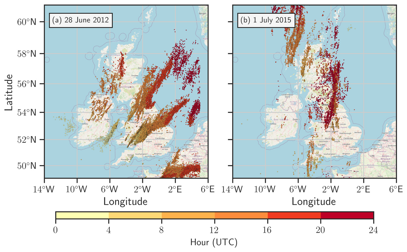
Figure 1 The spatial extent of lightning stroke occurrences as recorded by the ATDnet system (Gaffard et al., 2008) from 00:00 to 23:59 UTC on (a) 28 June 2012 and (b) 1 July 2015. Timestamps of all lightning strokes are categorised into 4 h intervals with times indicated by the colour scale. Lightning stroke data from Met Office from 2008–2016 (2017) and covering an area between (13.0° W and 5.0° E) and (49.0 and 61.0° N). Background map information from OSM (© OpenStreetMap contributors 2022. Distributed under the Open Data Commons Open Database License (ODbL) v1.0.).

Two days from this large dataset are selected, one for each case study. The first day of increased lightning activity was the 28 June 2012, and the corresponding synoptic analysis is provided by Clark and Webb (2013). The second day occurred on 1 July 2015 and was analysed by Lewis and Silkstone (2017). Both synoptic analyses give initiation and propagation details of three individual thunderstorms with auxiliary data from Doppler radars in the region and observations of other natural hazards. For both days, the spatial extent and propagation (in 4 h intervals) of the available lightning stroke data subsets are shown in Fig. 1. This figure will be discussed in more detail in Sect. 3.2 and 3.3.

3.2 Case study 1: Three supercell thunderstorms across English Midlands on 28 June 2012

The first case study (Fig. 1a) is based on a synoptic analysis of three supercell thunderstorms that crossed the English Midlands on 28 June 2012 during the 24 h period 00:00 to 23:59 UTC (Clark and Webb, 2013). The three thunderstorms are identified by their approximate initiation time and location, propagation path in descriptive terms and snapshots of the area around Doppler radar stations. Based on the synoptic analysis, we denote the three thunderstorms as Storm 1A, 1B and 1C, respectively, corresponding to supercells “A”, “B” and “C”. In this case study, for Storm 1B, the location and temporal information of the observed hail and tornado are used to assign lightning strokes to individual thunderstorms.

Using the available identifying information from the synoptic analysis and the lightning stroke location data, a total of N_L = 77 252 strokes are projected onto the OSGB 1936 (EPSG:27700) northing/easting coordinates. Points (i.e., position and time of observation) on these planes are selected based on the synoptic analysis, auxiliary data from Doppler radars in Clee Hill and Ingham, and observations of a tornado in Sleaford (Clark and Webb, 2013).

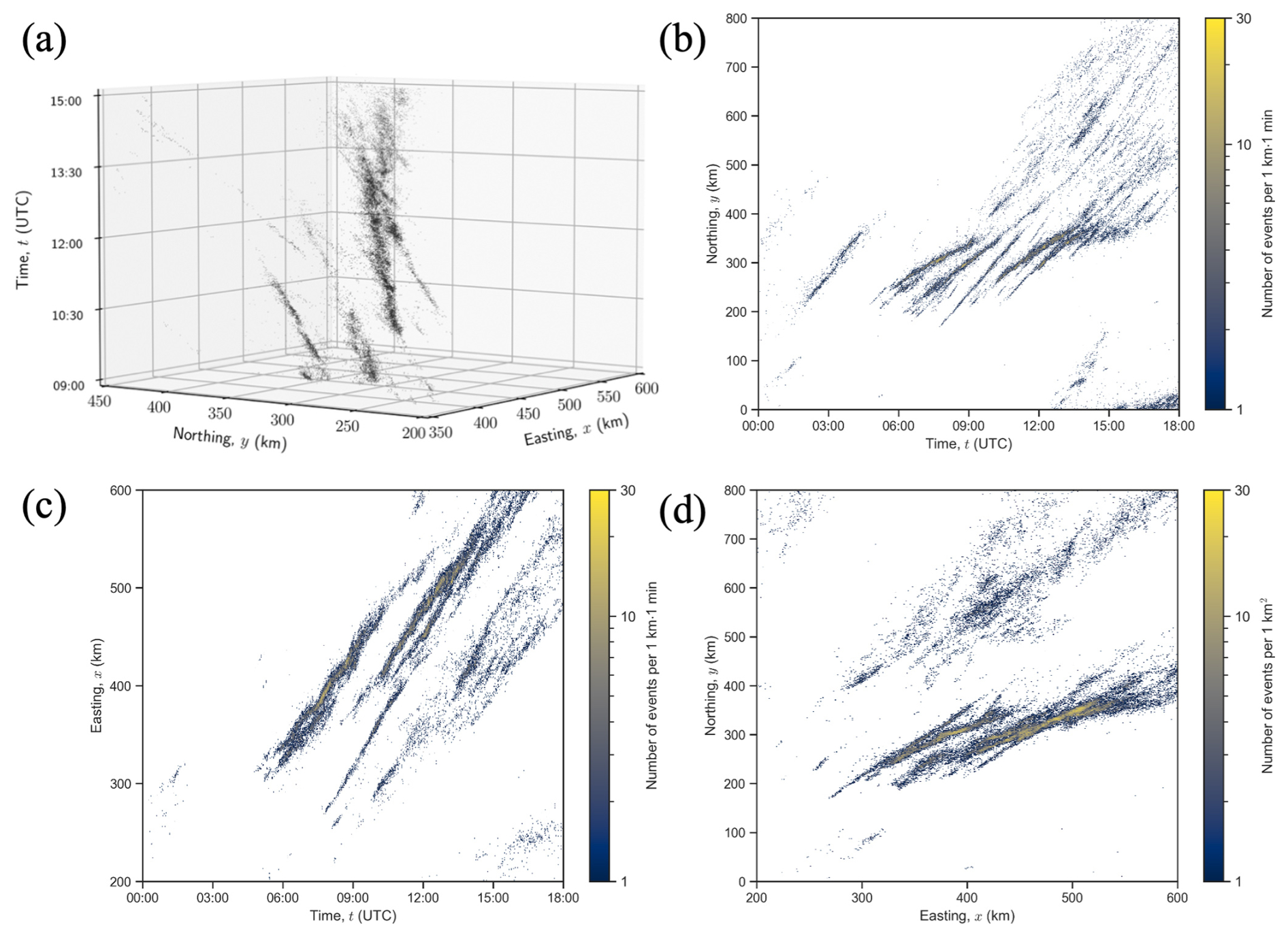
Figure 2 The lightning stroke data subset available for assignment to Storm 1B of the first case study in (a) three-dimensional, (b) two-dimensional northing-time, (c) two-dimensional easting-time and (d) two-dimensional northing easting views. The case study is based on a synoptic analysis of three supercell thunderstorms that crossed the English Midlands on 28 June 2012. For assignment and three-dimensional view, the spatial extent was restricted to x = (350, 600) km and y = (200, 450) km in the OSGB 1936 (EPSG:27700) easting/northing coordinates and the temporal extent from 09:00–15:00 UTC. All available lightning strokes are indicated as black scatter points in three-dimensional view and bin counts according to the colourscale in the two-dimensional views.

Using Storm 1B as an example for this assignment procedure, the initial limitation on the available lightning stroke point events is placed spatially and temporally. From the synoptic analysis (Clark and Webb, 2013), Storm 1B formed shortly after 10:00 UTC, started merging with smaller cells around 13:00 UTC and was tracked until 14:37 UTC. Spatially, the study area is focused on 350–600 km in easting and 200–450 km in northing coordinates. This spatial area includes the Clee Hill station, from which Storm 1B was always observed eastwards and places Sleaford close to the centroid of the study area. The lightning stroke data subset available for characterising Storm 1B is shown in Fig. 2 in three-dimensional view of all unassigned lightning strokes and two-dimensional bin count plots of the wider spatio-temporal domain.

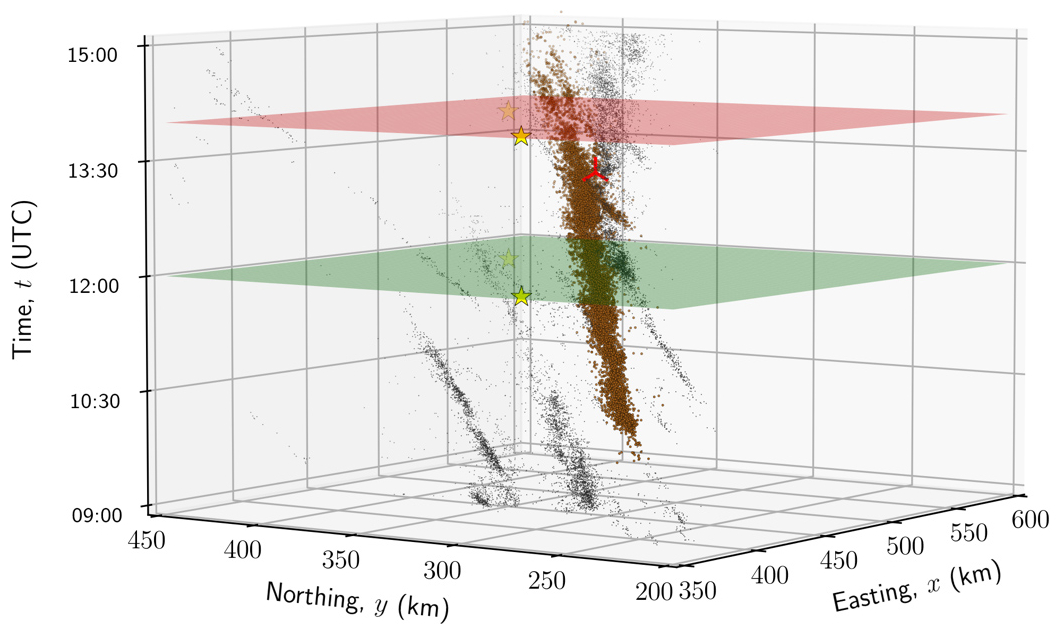
Figure 3 The first case study's assignment of lightning strokes to Storm 1B (dark brown scatter points). The locations of the Clee Hill and Ingham radar stations are marked as yellow star scatter points at two time points: 12:00 UTC (green plane) and 14:00 UTC (red plane). The location and first approximated time of occurrence (13:12 UTC) for the Sleaford tornado is marked as a red triangular line marker. The remaining unassigned lightning strokes are indicated as black scatter points.

Figure 2a shows the restricted three-dimensional domain for unassigned lightning strokes, while the various two-dimensional views of the lightning stroke bin counts in Fig. 2b–d indicate high stroke density regions within the unassigned dataset. Spatial and temporal scales can be further restricted from the auxiliary Doppler radar data available from the Clee Hill and Ingham stations. Snapshots of the Storm 1B location relative to these stations are available at 10:00, 12:00 and 14:00 UTC. Unprocessed reflectivity data is also available in 10 min intervals from 11:02–11:52 UTC in Clee Hill and in 10 or 15 min intervals from 12:42–13:37 UTC in Ingham. The snapshot frames move with the storm, so they are not useful in determining the exact location of Storm 1B relative to the stations, but they aid in understanding the storm's evolution. The lightning stroke data subset available for assigning lightning strokes to Storm 1B is shown in Fig. 3 with the relative positions of the Clee Hill and Ingham radar stations indicated.

Figure 3 shows that for the majority of the lightning strokes, assignment to Storm 1B was not complicated due to the clear separation of supercell thunderstorms, as noted in the synoptic analysis (Clark and Webb, 2013). Observational and tracking information available on the Sleaford tornado and hail further confirm the development and propagation of Storm 1B. The storm is tracked from 11:22 to 13:52 UTC through hail observation and radar data. The Sleaford tornado developed between 13:12 and 13:37 UTC. Both time intervals include the merge with smaller storm cells to the south of Storm 1B, complicating the exact assignment of lightning strokes.

The exact formation time was not indicated in the synoptic analysis but was set to be any time after 10:00 UTC due to Storm 1B not being identified at the 10:00 UTC Doppler radar snapshot. The noted merging of Storm 1B and local cells to the south at approximately 13:00 UTC is the main source of assignment uncertainty for individual lightning strokes. The exact termination time was also not noted in the synoptic analysis and was extended until 15:00 UTC to include any lightning strokes that still followed the general propagation direction of Storm 1B.

Table 1 Variables and their values used for the assignment procedure of individual lightning strokes to the six thunderstorms on 28 June 2012 (Storms 1A, 1B, 1C) and 1 July 2015 (Storms 2A, 2B, 2C).

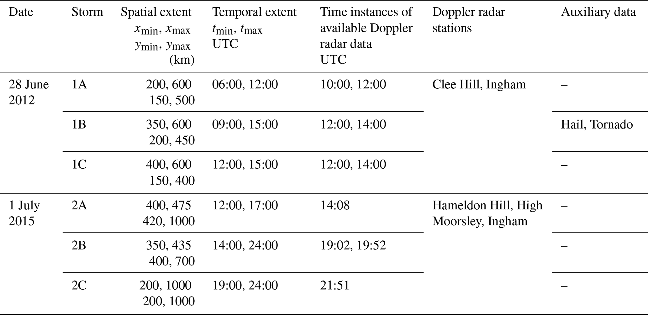
The summary of the initial spatial and temporal limitations on the lightning stroke dataset, the time instances used from Doppler radar data and any additional use of auxiliary data is shown in Table 1.

Figure 4 Spatial extent for 28 June 2012 of the lightning stroke occurrences as recorded by the ATDnet system over times intervals corresponding to the relevant synoptic analysis (Clark and Webb, 2013): (a) 09:30–10:30 UTC, (b) 10:30–11:30 UTC, (c) 11:30–12:30 UTC, (d) 12:30–13:30 UTC, (e) 13:30–14:30 UTC and (f) 14:30–15:30 UTC. Only lightning strokes assigned to any of the three selected thunderstorms (Storms 1A, 1B, 1C) are shown. Locations of relevant Doppler radar stations and the observed location of the Sleaford tornado are added as per the legend for direct comparison with synoptic analysis. Background map information from OSM (© OpenStreetMap contributors 2022. Distributed under the Open Data Commons Open Database License (ODbL) v1.0.).

To indicate the relative position of the assigned lightning strokes to the region's geography and their propagation, six 1 h intervals of the assigned lightning strokes are shown in Fig. 4. Additional three-dimensional plots of the assigned strokes can be seen in Appendix Fig. B1. The lightning strokes are separated by their assignment to a particular individual thunderstorm and are shown relative to the locations of the two Doppler radar stations and the observed tornado in Sleaford. These six intervals were chosen to cover the full temporal range of the lightning strokes as produced by the three thunderstorms.

As seen from Fig. 4, all three thunderstorms (Storms 1A, 1B, 1C) cross the Midlands in a SW–NE direction when viewed in the projected two-dimensional spatial domain. The locations of the Clee Hill and Ingham radar stations and the Sleaford tornado allow for direct comparison with relevant figures in the synoptic analysis. Three-dimensional plots of the assigned lightning strokes and all unassigned strokes can be found in Appendix Fig. B1.

3.3 Case study 2: Three structurally distinct severe thunderstorms across northern England on 1 July 2015

The second case study in Fig. 1b is based on a synoptic analysis of three structurally distinct severe thunderstorms that crossed the United Kingdom on 1 July 2015 (Lewis and Silkstone, 2017). The three thunderstorms are identified by their approximate initiation time and location, propagation path in descriptive terms and snapshots of the location around Doppler radar stations, as summarised in Table 1. We denote these three thunderstorms as Storms 2A, 2B and 2C, corresponding to the three storms identified in their synoptic analysis, which is identical to the identification algorithm used in the first case study.

Figure 5 Spatial extent for 1 July 2015 of the lightning stroke occurrences as recorded by the ATDnet system over times intervals corresponding to the relevant synoptic analysis (a) 12:30–13:30 UTC, (b) 13:30–14:30 UTC, (c) 18:30–19:30 UTC, (d) 19:30–20:30 UTC, (e) 20:30–21:30 UTC and (f) 21:30–22:30 UTC. Note that not every 1 h interval is plotted. Only lightning strokes assigned to any of the three selected thunderstorms (Storms 2A, 2B, 2C) are shown. Locations of relevant Doppler radar stations are added as per the legend for direct comparison with synoptic analysis. Background map information from OSM (© OpenStreetMap contributors 2022. Distributed under the Open Data Commons Open Database License (ODbL) v1.0.).

For this second case study, N_L = 12,521 strokes are recorded and projected onto the OSGB 1936 (EPSG:27700) northing/easting coordinates. The three-dimensional and two-dimension views of all lightning stroke points before assignment to individual storms are shown in Appendix Fig. C1. Planes are drawn to separate the lightning stroke dataset in the three-dimensional spatio-temporal space as for the first case study. Points on these planes are selected based on the synoptic analysis and the information from only the Doppler radar stations as noted in Table 1 as no other auxiliary natural hazard was observed in this case study. For this second case study, six 1 h intervals of the lightning strokes are chosen for spatial extent visualisation in Fig. 5. These intervals are not continuous due to the significant temporal gap between Storms 2A and 2B.

All three thunderstorms from 1 July 2015, when viewed in the projected two-dimensional spatial domain, cross northern England from south to north. The locations of the Hameldon Hill, High Moorsley and Ingham radar stations allow for direct comparison with relevant figures in the synoptic analysis. Three-dimensional plots of the assigned lightning strokes and all unassigned strokes recorded between 12:00 and 24:00 UTC are shown in Appendix Fig. B2.

4 Methods to characterise and model lightning variables in time and space

This section first introduces the physical variables used to characterise lightning strokes as spatio-temporal point events (Sect. 4.1). Three physical variables are then selected for characterisation and inclusion in a spatio-temporal model framework: lightning stroke inter-event occurrence time (Sect. 4.2), lightning stroke cluster movement speed (Sect. 4.3) and spatial spread (Sect. 4.4). Each of these variable subsections first presents the methodologies used to characterise the variable, then details the approach taken to incorporate the variable into a spatio-temporal point-event model framework. Then in Sect. 5, characterisation results for all three variables are presented and analysed, while in Sect. 6, the modelling approach is detailed and analysed, and examples of synthetic point-event datasets representative of lightning strokes are shown.

4.1 Lightning variables

Lightning as a natural hazard has been characterised by various methodologies, depending on the data type and purpose of the particular study. Characteristic variables depend on whether lightning data is analysed as a physical phenomenon (i.e. lightning flash) or as a point event in time and space. Each approach has distinct variables that can be characterised and used for various modelling approaches.

Lightning has been the subject of extensive research on the underlying physics that determine its initiation, propagation and related phenomena (Rakov, 2013; Dwyer and Uman, 2014). When using direct current measurements, the most commonly analysed variables include peak current, waveshape, the speed of the return stroke and the total flash charge (Chowdhuri et al., 2005). Using high-speed cameras, characterisation focuses on continuing current duration, time intervals between strokes, number of strokes per flash, total flash duration, flash multiplicity and inter-stroke intervals (Saba et al., 2006; Ballarotti et al., 2012). When analysing lightning as point events recorded by the lightning location systems (described in Sect. 3.1), the relevant variables are not directly physical. Since ATDnet detects individual strokes rather than complete flashes, the recorded point events correspond to stroke-level detections. Furthermore, as ATDnet predominantly detects CG return strokes via VLF sferics, the characterisable variables are constrained to those observable from stroke-level, CG-dominant data. This publication focuses on the statistical properties of the event process (identified at the individual storm level) more than on physical characteristics.

Variables such as lightning event count (either as lightning flash or stroke), density per month and/or per area unit, distribution per time unit, mean inter-stroke intervals, and multiplicity have been used to characterise lightning point events. Examples of global down to national spatial extent for these variables include the following studies:

• Global: Mezuman et al. (2014)

• Continental: Europe (Anderson and Klugmann, 2014; Enno et al., 2020)

• Regional: eastern Mediterranean (Yair et al., 2014), Mediterranean (Kotroni and Lagouvardos, 2016), Iberian Peninsula grid (Soriano et al., 2005), central and western Europe (Augenstein et al., 2025).

• National: Austria (Schulz et al., 2005); Poland (Taszarek et al., 2015).

In these studies, the spatial domain is gridded using either latitude/longitude; for example, a 0.1° × 0.1° grid (Kotroni and Lagouvardos, 2016); a 0.2° × 0.2° grid (Soriano et al., 2005; Anderson and Klugmann, 2014; Enno et al., 2020), or directly on Cartesian grid cells, for example, 10 km × 10 km cells (Taszarek et al., 2015; Augenstein et al., 2025). Temporal scales for these variables range from hourly, diurnal, monthly, seasonal to yearly characterisation.

These variables are characterised not only by spatial and/or temporal units but also by the use of additional lightning-specific nomenclature, the stratification of lightning events, or consideration of their relationship with other meteorological variables. For example, the variables can be characterised per thunderstorm day, when at least two flashes occurring within 20 km of the centre of a grid cell from 00:00 to 23:59 UTC (Enno et al., 2020). Variables can also be characterised after performing additional analyses on the spatio-temporal point event data, including aggregation of individual CG lightning strokes into ground strike points (Poelman et al., 2024) or clustering the point events into clustered convective events (Augenstein et al., 2025). Lightning events may also be stratified by whether they occur over land or sea areas (Mezuman et al., 2014) or characterised by their relationship with variables such as sea surface temperature (Kotroni and Lagouvardos, 2016).

This publication selects lightning variables to characterise the storm behaviour in both spatial and temporal domains. Initial data stratification occurred by grouping the lightning stroke data into individual thunderstorms (Sect. 3.2 and 3.3). For each thunderstorm, the behaviour in the temporal domain is first characterised by analysing the lightning stroke inter-event time variable Δτ (Sect. 4.2). In the spatial domain, the lightning stroke spread is analysed around an estimated thunderstorm movement track. This spread is characterised by easting and northing distances (Δx and Δy) from the movement track (Sect. 4.4). In the combined spatio-temporal domain, the estimated movement speed v of the individual thunderstorms producing the lightning strokes is characterised (Sect. 4.3).

4.2 Variable Δτ: Lightning stroke inter-event time

The first physical variable that is characterised and modelled is the inter-event occurrence time Δτ, with

$$\begin{array}{}\text{(1)}& \mathrm{\Delta }{\mathit{\tau }}_i=t_{i+\mathrm{1}}-t_i\mathrm{for}i=\mathrm{1},\mathrm{\dots },N-\mathrm{1}\end{array}$$

where t is time, and i an index on t representing discrete instances where events (lightning strokes) occur, noting that these events are not equally spaced in time. The inter-event time Δτ, as defined here, is computed from the full lightning stroke-level dataset recorded by ATDnet. It therefore represents two physically distinct processes: inter-stroke intervals, corresponding to successive current pulses within an individual flash and inter-flash intervals, related to the charge-replenishment processes within the storm. This distinction is discussed further in the context of the characterisation results (Sect. 5.1). For each thunderstorm, the characterisation process of the inter-event time data consists of descriptive analysis of inter-event occurrence time Δτ distribution. Distributions are analysed for each thunderstorm's complete lightning stroke dataset.

To include inter-event occurrence time as an input parameter for the spatio-temporal lightning stroke model (Sect. 6.1), the inter-event occurrence time Δτ data is processed in two steps:

Step 1.

Sampling from an empirical cumulative distribution function eCDF – synthetic inter-event time occurrence time values Δτ are generated to create a synthetic dataset without any temporal structure.

Step 2.

Re-indexing sampled inter-event times Δτ – temporal structure is added to the synthetic data by using autocorrelation function C(Δk) in inter-event occurrence times Δτ arranged in order of occurrence k from the individual thunderstorm datasets.

Inter-event time step 1 follows a methodology for non-parametric sampling from an empirical cumulative distribution (Ivezić et al., 2014). To generate a set of sampled inter-event occurrence time Δτ values from a real-world dataset, the Step 1 sampling methodology consists of three individual operations:

• 1.1

  Sorting – the set of inter-event occurrence times Δτ is sorted, and the rank of each time value is used to approximate the empirical cumulative distribution.

• 1.2

  Inverting cumulative distribution – the empirical cumulative distribution eCDF has the axes inverted to give the inverse empirical cumulative distribution.

• 1.3

  Spline fitting – a cubic spline fit to the inverse distribution is performed. As a result, a uniformly sampled x-axis value maps to a y-axis value, approximating the observed inter-event occurrence time probability distribution function.

Since the eCDF is constructed from the full inter-event time dataset, encompassing both inter-stroke and inter-flash intervals, the sampled synthetic values will reflect the combined bimodal distribution of both processes. As shown in Sect. 5.2, the close agreement between the plane-fit and linear-fit movement speed estimates suggests that this combination does not introduce a significant error into the characterisation and modelling of the inter-event time variable. The approach is therefore retained for its simplicity and its direct correspondence to the ATDnet stroke point output.

Inter-event time step 2 introduces temporal structure in the synthetic inter-event occurrence time Δτ dataset from the individual thunderstorms. Such information on the temporal structure can be given by applying the autocorrelation function to the N−1 inter-event occurrence times Δτ. The dataset from each individual thunderstorm is set in the order of occurrence k and the formulation of the autocorrelation function C(Δk) (Priestley, 1981) for a given lag Δk is

$$\begin{array}{}\text{(2)}& \begin{array}{rl}C\left(\mathrm{\Delta }k\right)=& {\displaystyle \frac{\mathrm{1}}{{\mathit{\sigma }}_{\mathrm{\Delta }\mathit{\tau }}^{\mathrm{2}}}}{\displaystyle \frac{\mathrm{1}}{N-\mathrm{1}-\mathrm{\Delta }k}}\\ & \times \sum _{k=\mathrm{1}}^{N-\mathrm{1}-\mathrm{\Delta }k}\left(\mathrm{\Delta }{\mathit{\tau }}_{k+\mathrm{\Delta }k}-\stackrel{\mathrm{‾}}{\mathrm{\Delta }\mathit{\tau }}\right)\left(\mathrm{\Delta }{\mathit{\tau }}_k-\stackrel{\mathrm{‾}}{\mathrm{\Delta }\mathit{\tau }}\right)\end{array}\end{array}$$

After Step 1, a synthetic inter-event occurrence time dataset T_S is generated with the same length as any of the individual thunderstorm inter-event occurrence time datasets (T_1A, …, T_2C). The methodology used in Step 2 for these two datasets consists of three individual operations:

• 2.1

  Sorting – the inter-event occurrence time datasets T_S and corresponding thunderstorm dataset are sorted by their value and ranked.

• 2.2

  Re-indexing – the synthetic dataset T_S has its inter-event occurrence times re-indexed to replicate the same ranking of inter-event occurrence times as the thunderstorm dataset.

• 2.3

  Autocorrelation comparison – autocorrelation function C(Δk) is applied to both datasets to ensure that the temporal structure of the thunderstorm data remains in the synthetic dataset T_S.

4.3 Variable v: Lightning stroke cluster movement speed

The second physical variable that can be characterised and modelled is the assumed constant movement speed v of the lightning strokes as a point-event cluster (i.e. representative of an individual thunderstorm). The approach to estimating the movement speed of the cluster is to perform a least-squares plane and linear fits to the lightning stroke data. The lightning stroke occurrence times t are assumed to depend on the easting x and northing y values as the thunderstorms producing these strokes move through the area and time of the study. Such a relationship between the dimensions can be expressed as

$$\left(\begin{array}{ccc}{x}_{\mathrm{1}}& y_{\mathrm{1}}& \mathrm{1}\\ \mathrm{⋮}& \mathrm{⋮}& \mathrm{⋮}\\ x_N& y_N& \mathrm{1}\end{array}\right)\left(\begin{array}{c}a\\ b\\ c\end{array}\right)=\left(\begin{array}{c}{t}_{\mathrm{1}}\\ \mathrm{⋮}\\ t_N\end{array}\right)$$

or

$$\begin{array}{}\text{(3)}& \mathbf{A}\mathit{\beta }=\mathit{t}\end{array}$$

where A is the matrix of the available spatial data (easting x and northing y values) as the first two columns. Vector β contains the three plane parameters that will be estimated by the best plane-fit. Vector t contains all the occurrence time t values. Finding the plane parameters in vector β is an over-determined problem (the number of equations outnumbers the unknowns), so the left pseudo-inverse of the matrix A is calculated. The least-squares approach then minimises the vertical (i.e. temporal) distance between the lightning strokes and the plane, returning the best plane-fit that can be thought of as the cross-section of the thunderstorm producing these strokes (Sect. 5.2).

As the best-fit plane coefficients are estimated from the least-squares fit, the movement speed v can be estimated as the inverse of the dip angle as given by these coefficients a and b

$$\begin{array}{}\text{(4)}& v={\displaystyle \frac{\mathrm{1}}{\sqrt{a^{\mathrm{2}}+b^{\mathrm{2}}}}}\end{array}$$

To further characterise the movement speed v after using the least-squares fit, the movement speed is returned with a goodness-of-fit calculation for each thunderstorm. This calculation consists of finding the root square mean error (RMSE) of the residuals between vector t and Aβ^∗ where β^∗ is the resulting parameter vector as found by the least-squares plane-fit. The full inter-event time dataset, which, as discussed in Sect. 4.2, contains a convolution of inter-stroke and inter-flash intervals, is used as input to both fitting approaches. As shown in Sect. 5.2, the close agreement between the plane-fit and linear-fit speed estimates across the storms suggests that this convolution does not introduce a significant error into the movement speed estimation. Both approaches operate in the geographic coordinate system (OSGB 1936/British National Grid), returning a movement speed that characterises the dominant motion of the storm.

A least-squares linear fit can also be used to estimate the movement speed v. This approach, applied for aftershock identification in seismology (Zaliapin and Ben-Zion, 2013), tornado touchdown location clustering and movement speed calculation (Malamud et al., 2016) and storm movement speed estimation (Finke, 1999), works in the spatio-temporal lag space {Δs, Δt}, where the spatial lag Δs and the temporal lag Δt between any two lightning strokes i = 1, …, N and j = 1, …, N−1 is the Euclidean distance and the time difference between them respectively

$$\begin{array}{}\text{(5)}& {\displaystyle }\mathrm{\Delta }{s}_{ij}=\sqrt{(x_i-x_j{)}^{\mathrm{2}}+(y_i-y_j{)}^{\mathrm{2}}}\text{(6)}& {\displaystyle }\mathrm{\Delta }{t}_{ij}=\left|t_i-t_j\right|\end{array}$$

As Δs_ij=Δs_ji and Δt_ij=Δt_ji, the duplicate data points are removed. It is assumed that in the spatio-temporal lag space {Δs, Δt}, the least-squares linear fit with an intercept set to pass through the origin returns the movement speed v from

$$\left(\begin{array}{c}\mathrm{\Delta }{t}_{\mathrm{1}}\\ \mathrm{⋮}\\ \mathrm{\Delta }{t}_{\frac{N(N-\mathrm{1})}{\mathrm{2}}}\end{array}\right)v=\left(\begin{array}{c}\mathrm{\Delta }{s}_{\mathrm{1}}\\ \mathrm{⋮}\\ \mathrm{\Delta }{s}_{\frac{N(N-\mathrm{1})}{\mathrm{2}}}\end{array}\right)$$

or

$$\begin{array}{}\text{(7)}& \mathit{T}v=\mathit{S}\end{array}$$

where T is the vector of all temporal and S is the vector of all spatial lags for N data points. The procedure that follows is the same as for Eq. (3). As input for the spatio-temporal lightning stroke model (Sect. 6.3), the movement speed v is used as a direct input parameter and assumed constant throughout the duration of the storm.

4.4 Variables Δx and Δy: the spatial spread of the lightning strokes as a cluster

The third physical variable that is characterised and modelled is the spatial spread of the lightning strokes as a cluster belonging to a particular thunderstorm. To characterise this variable, it is necessary to return an estimate of the track of the thunderstorm to have a reference against which to calculate the spatial spread. The spatial spread in the data can be characterised and modelled by two variables – easting and northing distances to the track (Δx and Δy). The calculation of these variables can be summarised in two steps:

1. Application of uniform filter – uniform filters are applied to easting x and northing y values in order of occurrence k to return a movement track.

2. Calculation of easting and northing distances – for each order of occurrence k, the easting and northing distances to the track (Δx and Δy) are calculated.

For spatial spread step 1, the movement track is assumed to be non-linear. It is estimated by applying a uniform linear filter on the easting/northing (x, y) coordinates (in the OSGB 1936/British National Grid) of the lightning stroke dataset in the order of occurrence k instead of real-time. The filter is used with a window size of Δw. When window size causes the average calculation at a given k to exceed the length of the northing and easting data vectors, the approach uses duplicates of the first or the last values accordingly. For spatial spread step 2, at each order of occurrence k, the calculation of (Δx, Δy) can be directly done with the easting/northing (x, y) and the estimated movement track coordinates (Sect. 5.3).

A methodology for fitting and sampling a bivariate normal distribution is implemented to include the easting and northing distances to the track (Δx and Δy) variables in the spatio-temporal lightning stroke model (Ivezić et al., 2014). This methodology is robust with respect to outliers in the data, given the approach's simplicity in estimating the movement track. To return the parameters of the bivariate normal distribution, the fitting process (i) uses the median instead of the mean and (ii) uses the interquartile range to estimate variances.

Once the distribution parameters are found, easting and northing distances to the track (Δx and Δy) are sampled directly from this distribution for implementation in the spatio-temporal lightning stroke model (Sect. 6.2). Therefore, the easting and northing distance distributions are sampled. Although a storm-relative coordinate system, decomposed into along-track and cross-track components, would provide a more physically interpretable description of the intrinsic spatial spread of lightning strokes around the storm track, the geographic coordinate system is retained here for two reasons. First, it serves as the direct input to the model without requiring a coordinate rotation. Second, the easting and northing distributions retain independent physical meaning, as they directly describe the spatial spread of lightning strokes in the coordinate system in which the model operates and in which the ATDnet data is recorded, making them directly comparable across different storm datasets without additional transformation.

5 Results of variable characterisation

This section presents the results of characterising the three lightning storm variables (inter-event times, movement speed, and distance to movement track) discussed in Sect. 4. These variable characterisations are for the six thunderstorms (28 June 2012: Storms 1A, 1B, 1C; 1 July 2015: Storms 2A, 2B, 2C) as detailed in Sect. 3.

5.1 Lightning inter-event times

We observe that for most storms, the time intervals at the beginning and end of the storm show systematically larger inter-event time values compared to the more central intervals. These larger values are physically consistent with lower flash rates during storm initiation and dissipation, when charge replenishment within the storm is less frequent, resulting in longer inter-flash periods in the combined inter-event time distribution. Therefore, we manually remove continuous time intervals from the lightning stroke datasets assigned to individual thunderstorms, where the inter-flash component of the inter-event time distribution shifts towards larger values, indicating reduced storm activity. This processing step is illustrated in Appendix D. This results in only a subset of each storm's stroke dataset being used to characterise the lightning inter-event times, corresponding to the storm's most active phase. If the time of occurrence of the first lightning stroke is t₁, the time axis is shifted to indicate the time since the first stroke t^′

$$\begin{array}{}\text{(8)}& t^{\prime }=t-t_{\mathrm{1}}\end{array}$$

After the removal of time periods, the final inter-event time Δτ dataset for further characterisation is used in terms of order of occurrence k. After the data processing to establish lightning stroke subsets with less ambiguity in their assignment to a particular thunderstorm, we can analyse the distribution of the inter-event times. Violin plots for the inter-event time Δτ subsets of all six thunderstorms are shown in Fig. 6.

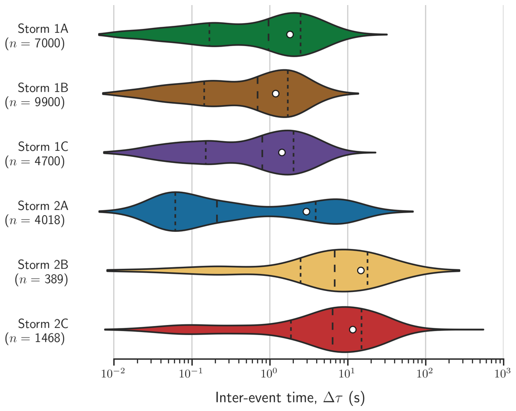
Figure 6 Violin plots of inter-event time Δτ distributions for all six selected thunderstorms. For each thunderstorm, the total number of observations after removing inter-event time values of the time-series is indicated by n, dotted lines denote the quartiles, and the white-dot represents the mean.

In Fig. 6, the inter-event times for all six thunderstorms cover four orders of magnitude, ranging from below 0.01 to over 100 s. For storms 1A, 1B and 1C, the empirical distributions cover similar ranges of 0.01 to 20–30 s. They show two peaks – a smaller one for values around 0.2 s and a larger one around 1–3 s and their quartiles are all within the same order of magnitude over all three storms. The similarity of both peaks across storms 1A, 1B and 1C suggests comparable flash rates and internal flash structure across these three storms.

The empirical distributions show more variability for storms 2A, 2B, and 2C. They include larger inter-event time values (more than 100 s) and show varying distribution shapes. Storm 2A has a larger peak around 0.05 s and the smaller one at around 7–8 s, which differs from the other five storms. The shorter peak at 0.05 s suggests shorter inter-stroke intervals, while the shift of the inter-flash peak towards 7–8 s compared to the 1–3 s range seen in the first case study is consistent with a lower flash rate for this storm. The empirical distributions for storms 2B and 2C are similar, with a clearer single peak centred at 8–10 s and covering the full range of inter-event times. The apparent merging of the two peaks into a single broader distribution may reflect a lower flash rate combined with shorter inter-stroke intervals. This reduces the separation between the two components of the combined distribution.

The bimodal structure of these distributions reflects two distinct physical processes captured within the ATDnet stroke-level detections. The shorter peak (∼ 0.2 s) is consistent with inter-stroke intervals, the time between successive current pulses within an individual flash, while the longer peak (1–3 s) is consistent with inter-flash periods, related to the charge replenishment processes within the storm (Rakov and Uman, 2003). This physical interpretation is acknowledged as a limitation of analysing inter-event times at the stroke level without explicit flash grouping: the resulting distribution is a convolution of two processes rather than a single well-defined quantity. Nevertheless, the combined inter-event time distribution remains a practically useful descriptor of storm activity, as it captures the aggregate temporal structure of stroke occurrence as recorded by ATDnet, which is the direct output of the detection network and the basis for the spatio-temporal model developed in this study.

5.2 Movement speed

The movement speed variable v (Sect. 4.3) is estimated using two complementary approaches. The first approach fits a least-squares plane directly to the spatio-temporal coordinates of the stroke dataset, with the results of the least-squares plane-fit to the lightning strokes assigned to storms 1B and 2A using the thunderstorm datasets as detailed in Sect. 5.1 shown in Fig. 7 (and all storms shown in Appendix E).

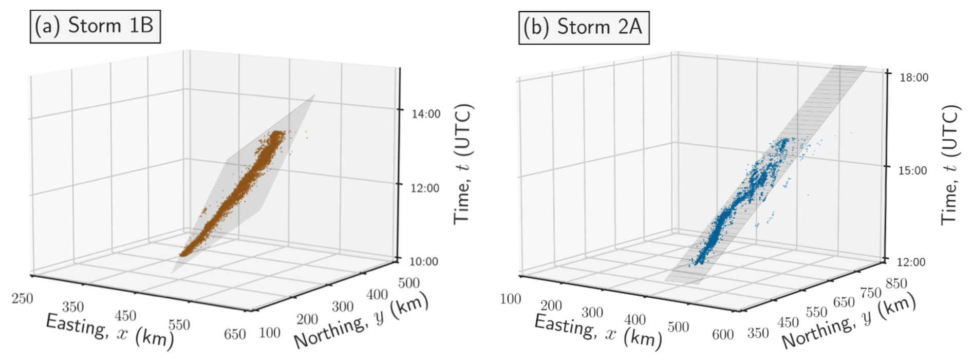
Figure 7 Least-squares plane-fit solution to the lightning stroke datasets for (a) Storm 1B (28 June 2012, n = 9901 events, v = 13 m s⁻¹ (47 km h⁻¹)), and (b) Storm 2A (1 July 2015, n = 4019 events, v = 30 m s⁻¹ (108 km h⁻¹)). Note that all three axes have different extents for each storm, while the ratio between the axes is constant. The best-fit plane solution is overlaid as a wireframe over the individual lightning strokes.

The second approach first converts the lightning-stroke data into spatio-temporal lag space {Δs, Δt} and fits a least-squares linear solution within that space, which allows the structure of the data to be examined in more detail. The resulting movement speed variable v estimates from the linear least-squares fits for storms 1A and 2C are shown in Fig. 8a and b, respectively. Together, Figs. 7 and 8 illustrate the degree to which the two methods agree and where internal storm complexity introduces additional variability into the speed estimate.

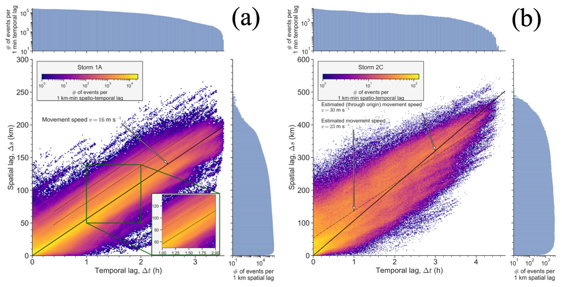
Figure 8 (a) Storm 1A (28 June 2012, n = 7001 events, v =  16 m s⁻¹ (59 km h⁻¹)) and (b) storm 2C (1 July 2015, n = 1469 events, v = 30 m s⁻¹ (108 km h⁻¹)) least-squares linear-fit solution and 2D count of lightning strokes per 1 km min in the spatio-temporal lag space. Bins are coloured according to the given logarithmic colour scale. The marginal bin counts per 1 km spatial lag and 1 min temporal lag are given above and to the right of the main plot. The abrupt vertical end of lightning stroke data in panel (a) at Δt = 3.45 h occurs due to the removal of inter-event time values. The solid black line indicates the best-fit linear line passing through the point of origin, while the dash-dotted line in panel (b) indicates the best-fit linear line. The two dashed lines in panel (a) parallel to the dark line, both set with identical v = 16 m s⁻¹ (59 km h⁻¹) indicate other areas of increased count density (bandings of orange pixels as seen in the enlarged panel in the lower right corner). These lines are set manually to emphasise the visually observable structure in the data.

The results for the movement speed v calculations from the plane-fit (Fig. 7 and Appendix E) and linear-fit (Fig. 8) and the RMSE of the residuals between stroke data and the best-fit plane-fit are indicated in Table 2.

Table 2 Results of least-squares plane-fit and linear-fit solutions to lightning stroke data for six UK thunderstorms.

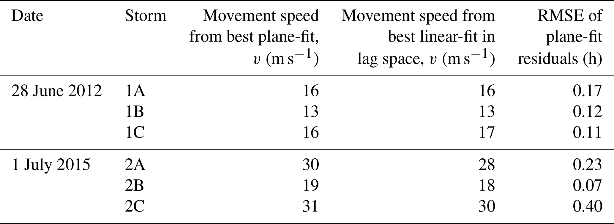
In Table 2, the calculated movement speeds from the two approaches vary between the two storm systems. Storms 1A, 1B and 1C return similar values in the range of 13–17 m s⁻¹ and Storms 2A, 2B and 2C show greater variability and higher values, ranging from 18–31 m s⁻¹. The goodness-of-fit estimation for the best plane-fit solutions shows low variability between the storms of the first case study (1A, 1B and 1C). For the second case study (2A, 2B and 2C), the variation is higher with storm 2B having the lowest RMSE of 0.07 h, while storm 2C has the highest at 0.40 h. The close agreement between the plane-fit and linear-fit speed estimates across the storms suggests that the inclusion of both inter-stroke and inter-flash intervals in the full inter-event time dataset does not introduce a significant error into the movement speed estimation.

In Fig. 8, the least-squares linear-fit solution in the spatio-temporal lag space returns more detailed information on the structure of each thunderstorm relative to using just a least-squares plane-fit (Fig. 7). In the spatio-temporal lag space, the storm's movement speed is initially assumed to correspond to a line passing through the point of origin. When looking at the structure of the 2D count plots (Fig. 8a for storm 1A, Fig. 8b for storm 2C), additional structures can be seen in the data that either do not pass through the point of origin or move at a different movement speed.

Initial observation of the 2D count plots shows bandings of pixels that indicate lines in the spatio-temporal lag space that do not pass through the point of origin but have a similar gradient (i.e. movement speed). This would indicate that the larger lightning stroke cluster (i.e. thunderstorm) consists of several smaller ones, each moving as part of the cluster with similar movement speeds (as seen by the dashed line examples in the enlarged panel for storm 1A in Fig. 8a).

It is also observed that bandings of pixels with different movement speeds within the same lightning stroke dataset exist, indicating the presence of smaller clusters in the data. The resulting movement speed value also depends on the assumption of the best-fit line passing through the origin (as seen by the dash-dotted and solid line examples for storm 2C in Fig. 8b). While these sub-structures reveal internal complexity within the storm datasets, the least-squares plane-fit applied in the spatio-temporal domain remains a valid and appropriate approach for estimating a bulk movement speed for each storm. The plane-fit is applied across the full spatio-temporal extent of the stroke dataset and therefore returns a single representative speed that characterises the dominant motion of the storm, rather than resolving individual sub-clusters of lightning strokes. This is consistent with the purpose of the movement speed parameter in the synthetic model developed in this study. The sub-cluster complexity identified in Fig. 8 is therefore best understood as a limitation on the precision of the movement speed estimate, reflected in the higher RMSE values for storm 2C, rather than as an invalidation of the plane-fit methodology itself.

5.3 Distance to the movement track

To investigate the distance to the movement track variable (Sect. 4.4), 2D spatial counts of lightning strokes per 1 km² of easting and northing distances for Storm 1A are shown in Fig. 9 (all storms shown in Appendix F).

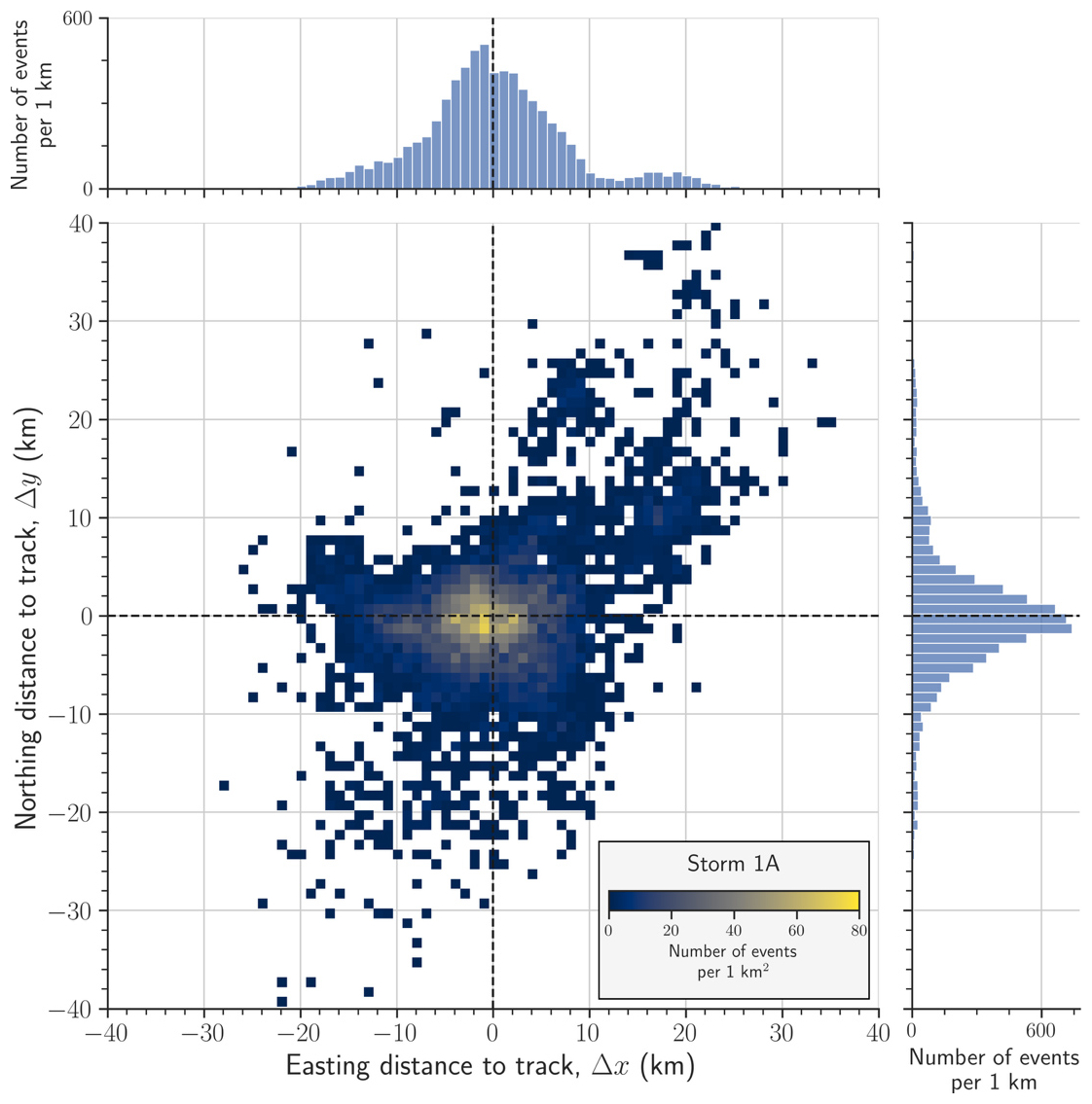
Figure 9 2D spatial count of lightning strokes per 1 km² of the easting and northing distances to the movement track in natural time k for lightning strokes in thunderstorm 1A (28 June 2012) for window sizes Δw=500 events. Only bins with more than 1 lightning stroke are coloured and the plot is zoomed onto [−40, 40] km intervals for both easting and northing distance. The marginal bin counts per 1 km are given for both northings and eastings.

In Fig. 9, the 2D spatial count ranges from 0–80 lightning strokes per 1 km², while the marginal bin counts reach values of approximately 450 and 650 lightning strokes per 1 km in the easting and the northing domain, respectively. The difference in the peak marginal bin counts between the easting and northing directions reflects the orientation of the storm's movement track relative to the geographic coordinate axes: as the movement track is not perfectly aligned with either axis, the spatial spread of strokes appears asymmetrically distributed between the two directions. This asymmetry is therefore a consequence of the storm's propagation direction rather than an intrinsic difference in the spatial structure of the lightning-stroke distribution along and across the storm track.

The highest 2D spatial and marginal bin count values are observed around the origin (x = 0, y = 0) km, consistent with the highest lightning-stroke density being concentrated along the movement track itself. The deviation in the 2D spatial and marginal bin counts from the origin is more pronounced in the positive ($+,+$) and negative ($-,-$) easting-northing distance quadrants, indicating that the spatial spread of strokes is not isotropic around the track. This diagonal elongation of the distribution in the 2D count plot is again consistent with the orientation of the movement track in geographic coordinates, as offsets along the direction of storm propagation project onto both the easting and northing axes simultaneously.

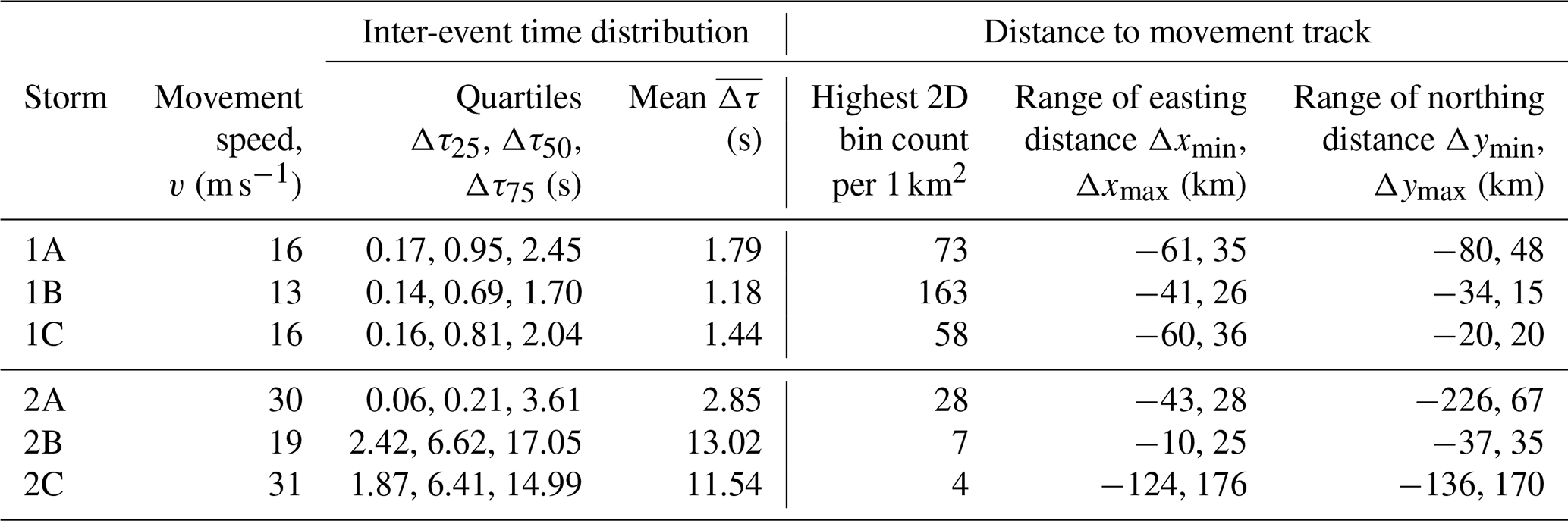
A summary of the characterisation results for all three lightning stroke variables, as presented in Sect. 5, is in Table 3.

Table 3 Summary of lightning stroke characterisation results.

6 Modelling lightning strokes

This section presents an approach to modelling lightning strokes as spatio-temporal point events, as mentioned in Sect. 2.2. The approach incorporates the three lightning storm variables (inter-event times, movement speed, distance to movement track) defined in Sect. 4 and characterised in Sect. 5 into a spatio-temporal model. The movement speed variable is set as a constant (including details from Sect. 4.3), while the approaches for incorporating inter-event time and distance to movement track are detailed in Sect. 6.1 and 6.2, respectively. The model details and procedure for creating a synthetic point-event dataset are described in Sect. 6.3, with a discussion on the limitations and uncertainties of this approach detailed in Sect. 7.

6.1 Sampling inter-event times

The goal is to sample a sequence of inter-event times that is representative of observations in real-world lightning datasets. We rely on the two steps procedure described in Sect. 4.2, using the datasets from the case studies presented in Sect. 3. In the first step, inter-event times are sampled without any temporal structure from a larger multi-storm dataset to obtain values that are not representative of just a single thunderstorm producing these events, but of a particular category of thunderstorms. From the synoptic analyses (Clark and Webb, 2013; Lewis and Silkstone, 2017) on the selected six thunderstorms (discussed in Sect. 3), these thunderstorms are categorised as supercell (storms 1A, 1B, 1C, 2B and 2C) or single cell (storm 2A). For example, we can select the supercell thunderstorms and combine the individual datasets to create a supercell dataset from which to sample inter-event times. As discussed in Sect. 4.2, the inter-event time dataset for each storm reflects both inter-stroke and inter-flash intervals, and the combined supercell dataset therefore reflects the aggregate temporal stroke structure across multiple supercell storms. While this means the sampled values are from two physically distinct processes, this is an inherent property of how events are defined in the ATDnet data and is consistent across all storms used in the combined supercell dataset.

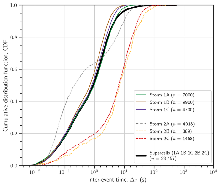
Figure 10 Cumulative distribution function (CDF) for the inter-event time Δτ for all six identified thunderstorms and the combined supercell thunderstorm dataset (black solid line). Individual storms within the storm system recorded on 28 June 2012 (Storms 1A, 1B and 1C) are indicated by solid lines, while those from storm system recorded on 1 July 2015 (Storms 2A, 2B and 2C) are indicated by dashed lines. Storm 2A is indicated by a grey line due to being single-cell thunderstorm and is not added to the supercell dataset.

A comparison between the cumulative distribution functions (CDFs) for all six individual thunderstorms and the common supercell dataset is shown in Fig. 10. The inter-event times are sampled from these CDFs following the methodology described in Sect. 4.2. The bimodal structure visible in the individual storm CDFs, reflecting the inter-stroke and inter-flash components of the distribution, is smoothed in the combined supercell CDF due to the averaging across storms with varying flash rates, producing a heavier tail than the individual storms from the first case study.

Figure 10 also shows the difference in the CDFs between the supercell thunderstorms and the single-cell one (storm 2A, dashed grey line), with two distinct peaks in the distribution for storm 2A. This is consistent with what we observed in the inter-event time distribution in Fig. 6. The difference between the CDFs of the supercells from both storm systems is also evident. For the storm system recorded on 28 June 2012 (storms 1A, 1B and 1C), the CDFs show similar behaviour to the storm system recorded on 1 July 2015 (storms 2B and 2C), but have a distribution peak smaller by an order of magnitude, consistent with the higher flash rates and consequently shorter inter-flash intervals.

Figure 10 also illustrates the contrast in the number of inter-event times n recorded during both storm systems. Storms 1A, 1B and 1C have a combined number of inter-event times n = 21 600, while the combined supercell dataset has n = 23 457 inter-event times. The supercell CDF closely resembles that of storms 1A, 1B and 1C with a heavier tail due to the presence of inter-event time data from storms 2B and 2C. This is a limitation of using the combined dataset, as the sampled values will be more representative of the first case study's flash rate regime than of the second.

Figure 11 Sampling, sorting and re-indexing procedure based on the combined supercell inter-event time Δτ dataset and thunderstorm (a) 1A, (b) 2C. The first panel (a1, b1) shows the original cut inter-event time-series in natural time k. The second panel (a2, b2) shows this sampled time-series being sorted and re-indexed based on the individual thunderstorm, where the indices of sorted time-series coincide between the two time-series. The third panel (a3, b3) shows the overlay between the original time-series and the sorted and re-indexed one in natural time k. The fourth panel (a4, b4) shows the autocorrelation comparison, including the confidence band.

The second step of the inter-event time generation is to introduce a temporal dynamic, by sorting and re-indexing a sampled inter-event time dataset from the first phase (detailed in Sect. 4.2). This phase introduces temporal structure in the sampled inter-event time dataset and allows us to generate an inter-event time sequence representative of real-world lightning data. The results of the two steps generation procedure for creating synthetic inter-event time datasets representative of storms 1A and 2C are shown in Fig. 11 (all storms are shown in Appendix G).

In Fig. 11, we see that the sampling, sorting and re-indexing procedure returns synthetic inter-event time datasets that are representative of supercell thunderstorms in value and representative of individual thunderstorms in their temporal structure. The difference between the inter-event time values between storms 1A, 1B, 1C, and storms 2B and 2C is evident in Fig. 11b3. The sampled, sorted and re-indexed dataset (grey line) have lower inter-event time values than original storm 2C (red line), which is expected from the discussion of Fig. 10. This reflects the dominance of the first case study's flash rate in the combined supercell dataset.

6.2 Sampling distances to the movement track

The approach to simulate a sample of distances from the movement track is detailed in Sect. 4.4 and the results of this sampling methodology is shown for storm 1A in Fig. 12 (the same figures for all storms are shown in Appendix F).

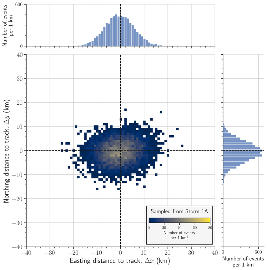
Figure 12 2D spatial count of lightning strokes per 1 km² of easting and northing distances to the movement track in natural time k for a bivariate Gaussian distribution based on storm 1A with window size Δw=500 events. Only bins with more than 1 lightning stroke are coloured and the plot is zoomed onto [−40, 40] km intervals for both easting and northing distance. The marginal bin counts per 1 km are given for both dimensions and the parameters of the bivariate Gaussian distribution are (μ_x = −0.46 km, μ_y = −0.61 km, σ_xx = 37.25 km², σ_yy = 17.83 km², σ_xy = 2.33 km²).

In Fig. 12, the 2D counts of lightning strokes show some clear differences with respect to the empirical ones in Fig. 9. This sampling approach, by using a bivariate Gaussian distribution, has not captured the minor peaks in northing and easting distance to track values. However, the marginal frequency for both easting and northing dimensions is very similar to the ones from the real-world data in Fig. 9, indicating that the overall spatial extent of the synthetic stroke distribution is well reproduced. However, the 2D counts reach values of only 50–60 events per 1 km², indicating that the bivariate Gaussian distribution produces a more diffused spatial concentration of strokes around the movement track than is observed empirically.

This is a limitation of fitting a bivariate Gaussian distribution to the data. The empirical distribution exhibits a non-trivial structure, including the diagonal elongation in the 2D count plot as discussed in Sect. 5.3, which reflects the orientation of the movement track in geographic coordinates, which a unimodal Gaussian cannot capture. The fitting methodology described in Sect. 4.4, which uses the median and interquartile range rather than the mean and variance, mitigates the influence of outliers, but is unable to capture the underlying distributional complexity.

6.3 Generating synthetic data from a representative spatio-temporal model

A spatio-temporal model of point events produced from a moving point source is used here to generate synthetic lightning stroke data. This model incorporates the lightning-stroke variables (described in Sect. 5) and the sampled distributions of the inter-event times (detailed in Sect. 6.1) and distances to the movement track (detailed in Sect. 6.2).

This spatio-temporal model generates a point-event dataset representative of lightning strokes (point events) produced by a single thunderstorm (moving point source). When combining multiple runs of this model, the point-event dataset would be representative of a storm system. A single run of this model can be described as the following procedure:

• Set constant variables:

  • Initiation point (x₀, y₀, t₀).

  • Movement speed v.

  • Movement direction α.

• Generate sampled sequences for:

  • inter-event time data,

  • distance to the movement track.

1. Place a point event – at the current track position, place a point event according to the first generated easting Δx₁ and northing Δy₁ distance to the movement track values.

2. Move along the track – starting from the initiation point, move in the movement direction with the set movement speed for a time period equal to the first inter-event time value Δτ₁.

3. Repeat steps 1 and 2 until the end of the sampled sequences.

The movement direction α and movement speed v are both constant throughout a single model run, which is a simplification of real thunderstorm behaviour. Thunderstorms may accelerate, decelerate or change direction over their lifetime. This simplification is consistent with the straight-line plane-fit methodology used to estimate v in Sect. 4.3, which returns a single speed and direction representative of the dominant storm motion.

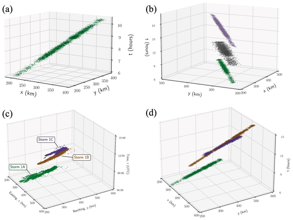
Figure 13 (a) A single run of the spatio-temporal model to produce a lightning stroke dataset representative of storm 1A and a (b) synthetic three-storm system with varying spatial spread parameters. In panel (a), the initiation point is set at (x₀ = 200 km, y₀ = 200 km, t₀ = 6 h). The movement speed value is set at v = 16 m s⁻¹ as per the characterisation of the movement speed variable (Appendix Fig. E1). Inter-event times are sampled, sorted and re-indexed as per Fig. 11a1–a4. Easting and northing distances are sampled from the bivariate Gaussian distribution shown in Fig. 12. The first (green) storm is identical to panel (a) with bivariate Gaussian distribution parameter set from parameter characterisation (μ_x = −0.46 km, μ_y = −0.61 km, σ_xx = 37.25 km², σ_yy = 17.83 km², σ_xy = 2.33 km²). The second (dark grey) storm is based on bivariate Gaussian distribution with parameters (μ_x = 0, μ_y = 0, σ_xx = 100 km², σ_yy = 100 km², ρ = 0). The third (purple) storm has parameters (μ_x = 0, μ_y = 0, σ_xx = 100 km², σ_yy = 100 km², ρ = 0.9). For all storms, the movement speed is kept the same at v = 16 m s⁻¹ and inter-event time distribution is representative of storm 1A. A synthetic three-storm system (d) that consists of individual synthetic storms representative of Storms 1A, 1B and 1C from case study 1 (c). The movement speed values, re-indexed inter-event time values and spatial spread parameter distributions are selected for each storm using Table 3.

As discussed in Sect. 6.1 and 6.2, it is necessary to select a particular thunderstorm to sample the sequences of the inter-event times and distances from the track. A single run of the model to produce a lightning stroke dataset representative of storm 1A is shown in Fig. 13a and this run with an additional two runs of the model to form a “three storm system” shown in Fig. 13b. For the two additional model runs, the bivariate Gaussian distribution for the distance to the movement track variable is set with parameters (μ_x = 0, μ_y = 0, σ_xx = 100 km², σ_yy = 100 km²). The correlation parameter for the two additional runs is set at ρ = 0 and ρ = 0.9. No other variables or sampled sequences are changed for these model runs, allowing for the effect of the spatial spread parameter alone to be examined.

In Fig. 13, the flexibility of the model is demonstrated. A model run representative of a lightning stroke dataset produced by a thunderstorm is compared with additional runs in which only one lightning variable is changed. This allows the visual effect of end-member values for the particular variable to be examined. Additional model runs are representative of storms 1B and 1C, are generated to create a synthetic storm system representative of the first case study (Sect. 3.2), is shown in Fig. 13d. The synthetic storm system in Fig. 13d is generated using variables and sampled sequences representative of the lightning-stroke datasets from case study 1 as seen in Fig. 13c. The synthetic lightning stroke datasets propagate further in the spatial and temporal domains than the real-world datasets on which they are based. This is partly a consequence of the heavy tail of the combined supercell inter-event time dataset discussed in Sect. 6.1: sampling from this dataset introduces occasional large inter-event time values from the second case study storms, causing the synthetic storm to persist longer than the individual real-world storm on which it is based. We also note the assumption of straight-line propagation of the moving point source (thunderstorm) producing the individual point events, which is a simplification as discussed in the modelling approach to the spatial spread of the lightning strokes (Sect. 4.4).

7 Discussion

The characterisation and modelling (Sect. 5) and simulative (Sect. 6) aspects in this study of lightning strokes as point events generated by a moving source were based on two selected case studies of increased lightning activity (Sect. 3). This section discusses the following five aspects related to our modelling approach for lightning strokes: (A) relevance to different categories of thunderstorms, (B) lightning inter-event time characterisation, (C) estimating lightning cluster movement speeds, (D) estimating lightning cluster spatial spread, and (E) overall motivation and limitations.

• A.

  Relevance of our modelling approach for lightning strokes associated with different categories of thunderstorms. Each case study described a storm system consisting of three thunderstorms over a single day of the observed increase in storm activity. To characterise and model these thunderstorms, lightning stroke data for both days were gathered by the ATDnet LLS over the United Kingdom. The two case studies categorised five of the six identified thunderstorms as supercells. In other characterisations of lightning strokes as point-event studies (e.g. Enno et al., 2020; Mezuman et al., 2014; Anderson and Klugmann, 2014), each study's characterisations added to lightning climatology research without emphasis on specific thunderstorm types. This highlights the novelty of our approach and the potential for further research to characterise specific storm types. In Anderson and Klugmann (2014), the diurnal flash density characterisation included case study 1 (Sect. 3.2), but did not separate the characterisation results for individual thunderstorms. Although five out of the six thunderstorms in these case studies were supercells, there were clear differences in their characterisation results (e.g. empirical distribution differences in Fig. 10), indicating a further research direction into identifying and characterising further case studies of more varied thunderstorm categories.

• B.

  Generality of our approach for lightning inter-event time characterisation. While applicable to these case studies, it is acknowledged that the characterisation results for lightning associated with given thunderstorms cannot be generalised to all thunderstorms due to variations in characterisation results across studies. To address this lack of generality in lightning associated with thunderstorm characterisation, we created a supercell inter-event time Δτ dataset (Fig. 10) to model Δτ. We acknowledge that the removal of inter-event times (Appendix D) is trivial and not based on quantitative approach and thus the supercell dataset could be improved. The inter-event time dataset for each storm captures both inter-stroke and inter-flash intervals, with the combined supercell dataset reflecting their aggregate temporal stroke structure across multiple supercell storms. The limitation in modelling this particular variable is the discrepancy in dataset size between the case studies (i.e., the first case study has n = 21 600 lightning strokes, while the combined supercell dataset has n = 23 457 strokes). The values sampled from this supercell dataset are more representative of the first case study. In contrast, the larger Δτ values for the second case study resulted in a heavier tail for the combined distribution. The characterisation results yield value intervals similar to those of other studies focusing on physical variable characterisation. Inter-event time values range from below 0.01 to over 100 s for individual storms from both case studies. For storms 1A, 1B and 1C, the empirical distributions cover a range of 0.01 to 20–30 s. The shorter peak of the bimodal distribution (∼ 0.2 s) is consistent with published inter-stroke interval means: Ballarotti et al. (2012), a study conducted over Vale do Paraíba, Brazil using high-speed cameras, returned an arithmetic mean for the inter-stroke time interval of 92 ms (millisecond). In Saba et al. (2006) over southern Brazil, a dataset of 608 inter-stroke time intervals had an arithmetic mean of 83 ms. Over different study areas, such as the eastern Mediterranean and Israel (Yair et al., 2014) and Arizona, the United States (Stall et al., 2009), the mean inter-stroke interval was found to be 93 and 98 or 84 ms, respectively (depending on whether strokes used a pre-existing lightning channel or created new ground contacts). These results are in good agreement with the inter-stroke component of the inter-event time distributions found in this paper for storms 1A, 1B, 1C.

• C.

  Estimating lightning cluster movement speed. Speed values for storms 1A–1C, were similar, ranging between 13–17 m s⁻¹ from the best plane fit and the linear fit in lag space of lightning associated with each storm. For storms 2A and 2C, the two methodologies returned higher movement speed values of 28–31 m s⁻¹. Storm 2B had a value range of 18–19 m s⁻¹, similar to the first case study. The novelty of the approach presented here lies not in the use of lightning data for storm motion estimation per se, but in the specific methodology of estimating movement speed from the spatio-temporal lag space of stroke-level point-event data recorded by ATDnet, for which equivalent published approaches are not currently known to the authors. The close agreement between the plane-fit and linear-fit speed estimates across all storms supports the robustness of the approach and indicates that including both inter-stroke and inter-flash intervals in the full inter-event time dataset does not introduce a significant bias into the movement speed estimation, as discussed in Sect. 4.3. Such estimates are usually based on two-dimensional radar reflectivity data (e.g. the automated cell detection algorithm KONRAD (Lang, 2001) used in Wapler and James (2015) to calculate the movement speed of thunderstorms over Central Europe spanning from 2007–2012, which require additional data sources beyond the lightning-stroke dataset itself. They used 29 categories to classify the observed thunderstorms based on regional synoptic characteristics over Central Europe. Over these defined thunderstorm categories, the median movement speeds (within each category) of all the observed thunderstorms varied from 6–18 m s⁻¹. Over North Dakota, the United States in Mohee and Miller (2010), the thunderstorm climatology was presented for a time period of 2002–2006. The thunderstorms were not categorised into various synoptic categories but were instead stratified temporally based on the month. The movement speed values ranged from 15.4–20.4 m s⁻¹. Both studies confirm that for the supercell thunderstorms in the first case study, their movement speed values fall within reasonable range found in other studies.

• D.

  Estimating lightning cluster spatial spread. For the distance to the lightning cluster movement track, there was significant bias in the spatial spread of the lightning strokes as a cluster of point events (Sect. 4.4). Therefore, the bivariate Gaussian distribution was selected to model the data for simplicity. We are not aware of any other peer-reviewed publications estimating the distance to the lightning cluster movement track directly from stroke-level point-event data. Movement track estimates are usually done by temporal windows. In Strauss et al. (2013), additional precipitation data were used to estimate storm cells and their centroid locations over 10 min intervals were used as points along the movement tracks. In Kunz et al. (2020), 26 000 severe convective storm tracks between 2005 and 2014 were estimated from two-dimensional radar reflectivity data. They estimated the storm tracks by using a modified version of the cell-tracking algorithm TRACE3D (Handwerker, 2002). Such approaches were deemed too complex as the objective of the characterisation process is to provide an estimate for the spatial spread parameter for the models. The characterisation of the spatial spread variable (Fig. 9) showed a non-trivial empirical distribution. Still, no other potential distributions were evaluated on the data, given the primary objective of providing a practical input distribution for the synthetic model, and this is a potential future research direction. Another potential research direction is modelling the movement track with a curve rather than a straight line. We followed this approach when characterising the spatial spread (Sect. 4.4), but it would be useful to incorporate this in the generative model (Sect. 6). We recognise that a storm-relative coordinate framework, consisting of along-track and cross-track distances, could offer a more physically meaningful interpretation of the lightning spatial structure, allowing for comparison of intrinsic storm width and length independently of storm propagation direction. However, adopting such a transformation introduces substantive additional uncertainty, as it relies on the assumption of a linear storm track, unless a significantly more complex model is chosen for storm track identification. Therefore, any deviation from straight-line propagation would cause the along-track and cross-track components to be misaligned with the true storm-relative axes, propagating error into the spatial spread estimates. The geographic coordinate system is retained here as the more robust choice for the purposes of the generative model. The characterisation of the spatial spread in storm-relative coordinates, particularly if combined with improved non-linear track estimation, is identified as a direction for future work, as it would allow the along-track and cross-track spread to be interpreted independently of storm orientation and compared systematically across storms of different propagation directions.

• E.

  Motivation for the implemented modelling approach and its limitations. The motivation for modelling lightning strokes was to create synthetic point-event datasets generated by a moving point source representative of “real-world” lightning stroke data. Modelling and sampling approaches were proposed for the inter-event times and distances from the movement track (Sect. 6). No direct sampling of characterised variables was implemented in the spatio-temporal model of lightning strokes as point events in Finke (1999), and the data-driven approach adopted here represents a methodological advance over that framework. The approach to designing the spatio-temporal model was selected to have complete control over the variables and sampled sequences. The model can generate any point-event datasets produced by a moving source, depending on the sets of input parameters. The model also has clear procedures for propagating the moving point source (i.e. a thunderstorm) and placing point events (i.e. lightning strokes) along this point source.

Several simplifying assumptions and limitations of the model are acknowledged. The movement speed and direction are both assumed to be constant throughout a single model run, which does not capture the acceleration, deceleration or directional changes that real thunderstorms may undergo over their lifetimes. The spatial spread is modelled using a single bivariate Gaussian distribution fitted to the full stroke dataset, which does not resolve the cluster structure identified in the spatio-temporal lag space analysis (Sect. 5.2) nor the non-trivial distributional shape of the real-world distance to movement track data (Sect. 6.2). The inter-event time dataset used as input is a combination of inter-stroke and inter-flash intervals, and while the agreement between the two speed estimation methods suggests this does not materially affect the movement speed estimate, it means that the temporal structure of the synthetic dataset reflects both processes simultaneously rather than either one in isolation. Finally, the straight-line propagation assumption will introduce increasing positional error over the duration of longer model runs, as discussed in Sect. 4.4.

Despite these limitations and its overall simplicity, this model establishes a transparent and directly controllable framework for producing synthetic lightning-stroke data representative of particular case studies, with clear procedures for each model component. This allows for the simulation of a specific category of thunderstorm and provides a foundation for extending the framework to other natural hazards that can be characterised as point events produced by a moving source, such as tornado touchdown locations.

8 Conclusions

This study presents a comprehensive characterisation and modelling of thunderstorm-associated lightning strokes as spatio-temporal point events. It focuses on two thunderstorm systems over the United Kingdom as case studies for demonstrating the methodological contribution of characterising and modelling lightning strokes as spatio-temporal point events. Through detailed analysis of these two real-world datasets, we successfully identified and characterised the movement speed, inter-event time distribution, and spatial spread of lightning strokes for six individual thunderstorms. The lightning-stroke data used in this study was recorded by the ATDnet VLF lightning location system operated by the Met Office, which detects individual strokes, the discrete current pulses within a complete lightning flash, rather than flashes directly. This distinction affects the quantitative interpretation of the characterisation results throughout the study.

Our findings highlight distinct patterns in lightning stroke behaviour, such as the following: lightning cluster movement speeds ranging from 13–17 and 18–31 m s⁻¹for the two storm systems, respectively; a bimodal inter-event time distribution covering four orders of magnitude, with a shorter peak around 0.2 s consistent with inter-stroke intervals and a longer peak between 1–10 s consistent with inter-flash intervals, reflecting the two physically distinct processes captured within the ATDnet stroke-level detections; and a spatial spread of lightning stroke clusters with typical distances up to 80 km from the storm track, with one outlier reaching 226 km.

The synthetic lightning stroke model developed in this study provides a directly controllable and robust tool for generating representative point-event datasets. This model, which incorporates empirically derived parameters from real-world data, offers valuable insights for simulating lightning stroke events and can aid in improving forecasting models for lightning-related hazards. Our research contributes to a deeper understanding of lightning stroke dynamics and offers a methodological framework applicable to other spatio-temporal natural hazard events characterised as point events produced by a moving source, such as tornado touchdown locations. Future work could expand on this foundation by evaluating alternative distribution fits for the spatial spread variable, characterising the spatial spread in storm-relative coordinates decomposed into along-track and cross-track components, incorporating non-linear storm-track modelling and exploring different storm types and regions to further refine and confront the model.

In conclusion, this study enhances our ability to characterise and model lightning strokes as spatio-temporal point events, with the stroke/flash distinction shown to be physically meaningful for interpreting the bimodal inter-event time distribution and its temporal evolution. The framework established here offers implications for hazard assessment and risk management in meteorological studies and provides a replicable methodology for extending spatio-temporal point process modelling to other natural hazards.

Appendix A: List of publications on modelling natural hazards as point events

Table A1 Summary Table of publications on using spatio-temporal point process models to model natural hazard processes.

Appendix B: Spatial extent and propagation of the lightning stroke occurrences for both storm systems

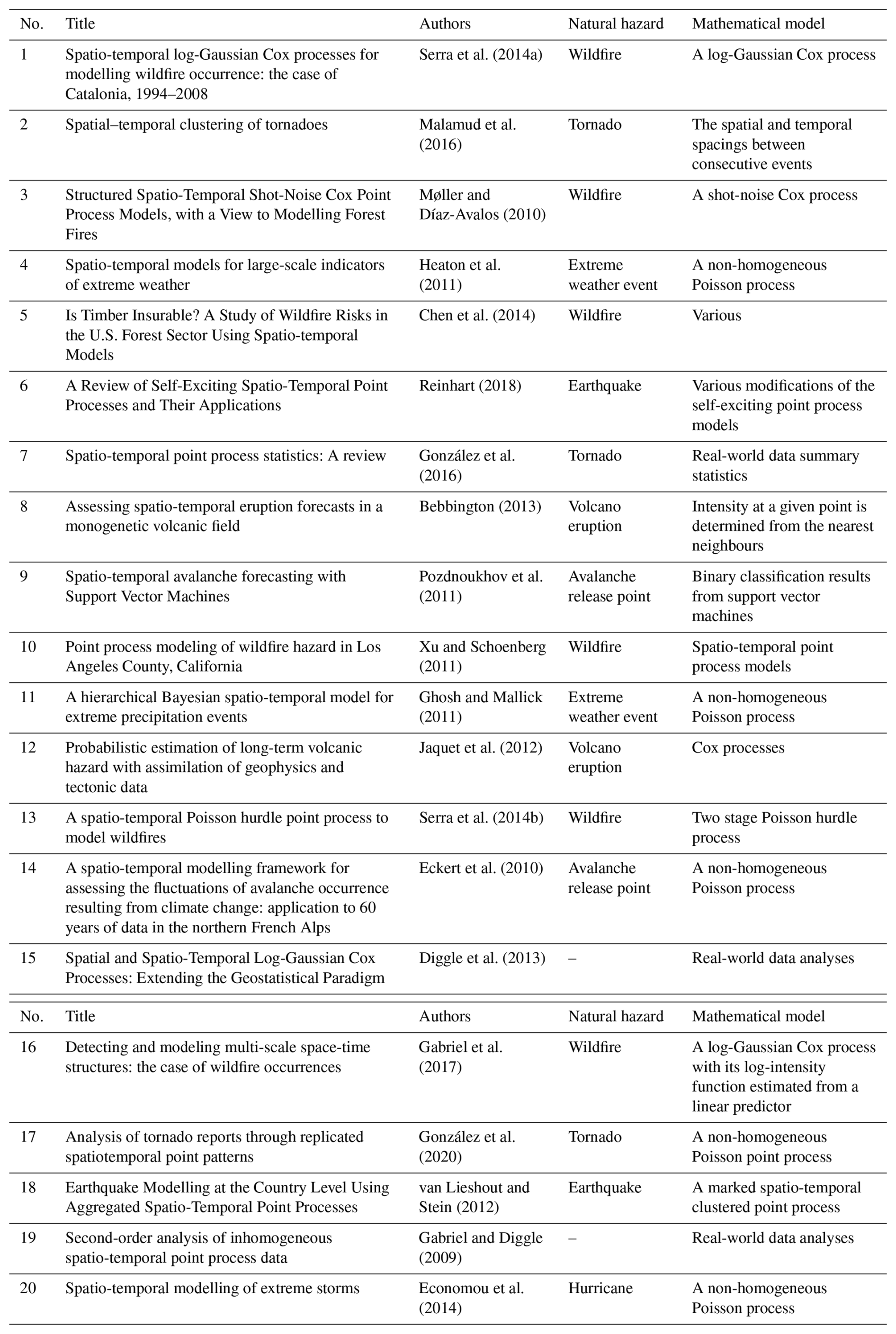
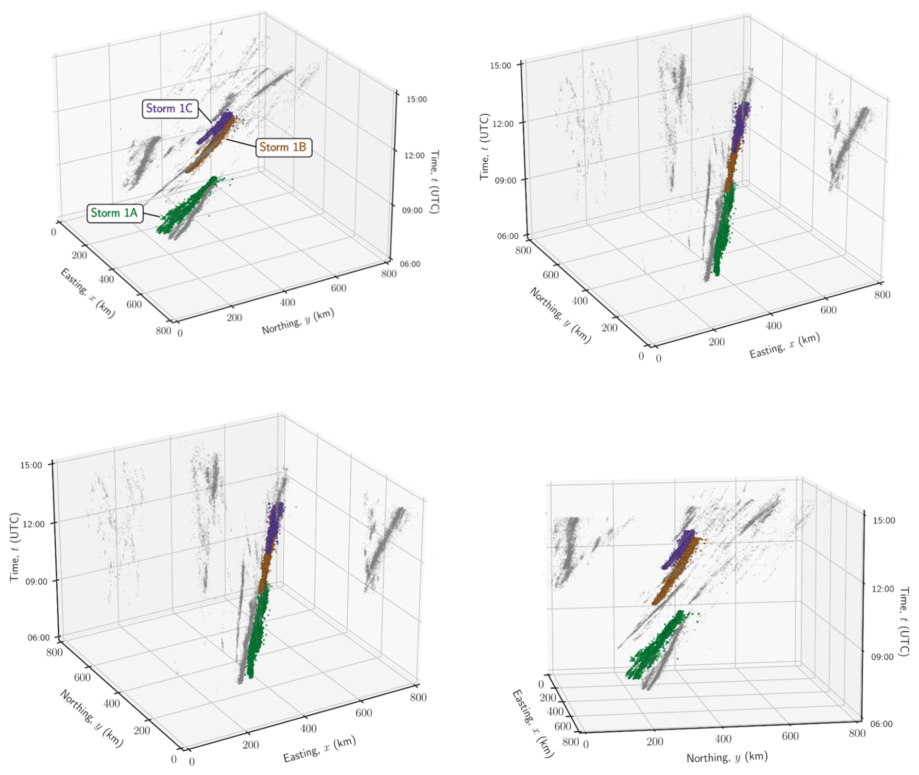
Figure B1 Angles of the 3D spatial extent and propagation of the lightning stroke occurrences plots in Fig. 4. Lightning strokes are projected onto the OSGB 1936/British National Grid northing/easting coordinates, assigned to the identified thunderstorms corresponding to the relevant synoptic analysis.

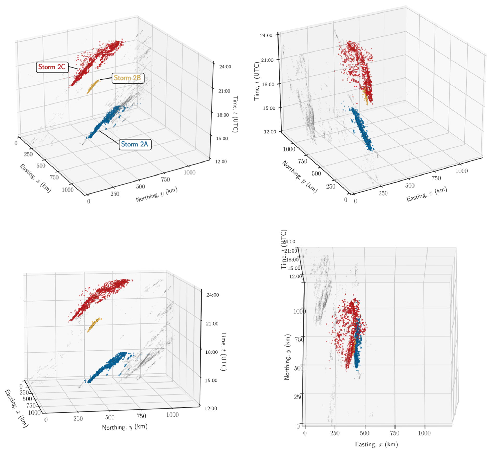
Figure B2 Angles of the 3D spatial extent and propagation of the lightning stroke occurrences plots in Fig. 5. Lightning strokes are projected onto the OSGB 1936/British National Grid northing/easting coordinates, assigned to the identified thunderstorms corresponding to the relevant synoptic analysis.

Appendix C: 3D and 2D views of unassigned lightning stroke data for second case study

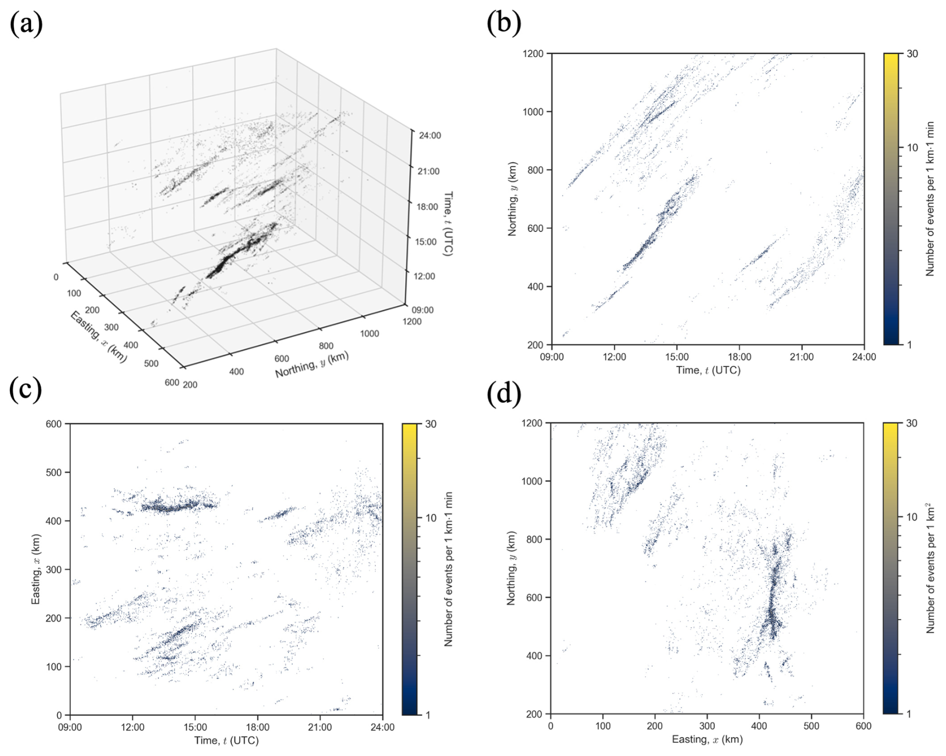
Figure C1 The lightning stroke data available for assignment to storms of the second case study in (a) three-dimensional, (b) two-dimensional northing-time, (c) two-dimensional easting-time and (d) two-dimensional northing easting views. Available lightning strokes are indicated as black scatter points in three-dimensional view and bin counts according to the colourscale in the two-dimensional views.

Appendix D: Cutting time series of inter-event times

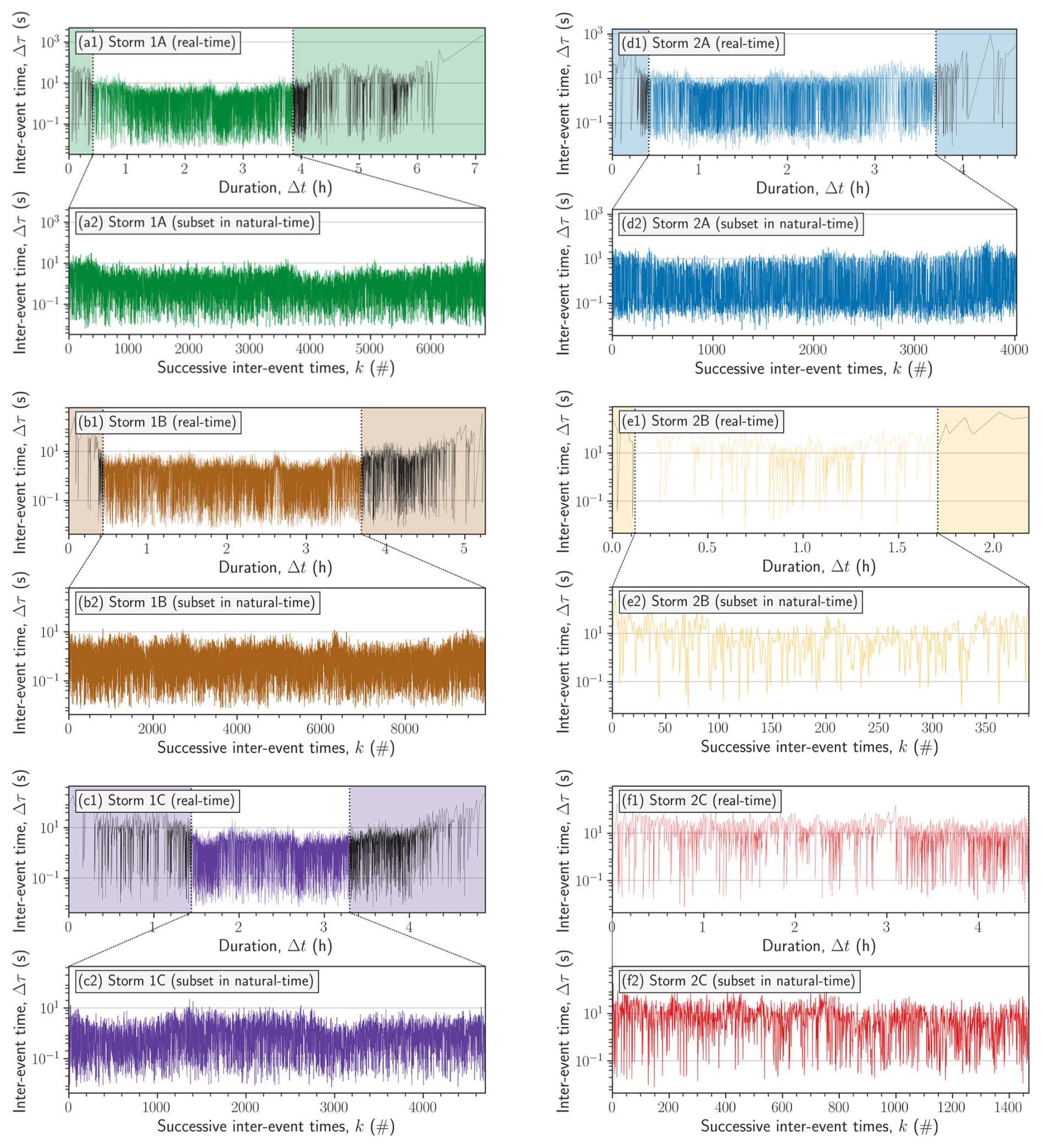
Figure D1 Subplots showing the cutting of inter-event time Δτ time-series in real-time t (removal of black line in upper panel) and the subsequent inter-event time time-series in natural time k (lower panel) for thunderstorms (a1, a2) 1A, (b1, b2) 1B, (c1, c2) 1C, (d1, d2) 2A, (e1, e2) 2B and (f1, f2) 2C.

Appendix E: Least-squares plane-fit solution to the lightning stroke datasets

Figure E1 Least-squares plane-fit solution to the lightning stroke datasets for thunderstorms (a) 1A, (b) 1B, (c) 1C, (d) 2A, (e) 2B and (f) 2C. The colour scheme for lightning strokes of each storm is consistent with Figs. 4 and 5 and the best-fit plane is drawn as grey wireframe. Note that all three axes have different extents for each storm, while the ratio between the axes is constant.

Appendix F: Bivariate Gaussian fit to spatial spread variable to sample easting and northing distances

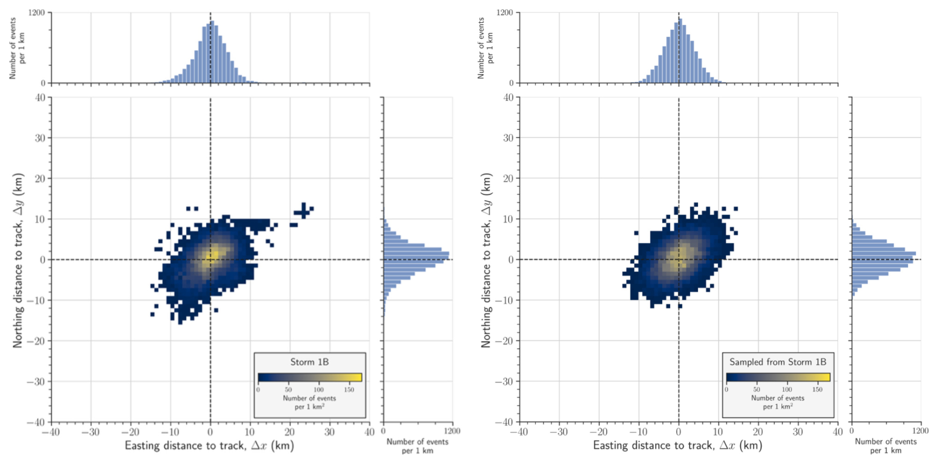
Figure F1 2D spatial count of lightning strokes per 1 km² of easting and northing distances to the movement track in natural time k for thunderstorm 1B (left panel) and for a bivariate Gaussian distribution based on thunderstorm 1B (right panel) for window sizes Δw=500. Only bins with more than 1 lightning stroke are coloured and the plot is zoomed onto [−40, 40] km intervals for both easting and northing distance. The marginal bin counts per 1 km are given for both dimensions.

Figure F2 2D spatial count of lightning strokes per 1 km² of easting and northing distances to the movement track in natural time k for thunderstorm 1C (left panel) and for a bivariate Gaussian distribution based on thunderstorm 1C (right panel) for window sizes Δw=500. Only bins with more than 1 lightning stroke are coloured and the plot is zoomed onto [−40, 40] km intervals for both easting and northing distance. The marginal bin counts per 1 km are given for both dimensions.

Figure F3 2D spatial count of lightning strokes per 1 km² of easting and northing distances to the movement track in natural time k for thunderstorm 2A (left panel) and for a bivariate Gaussian distribution based on thunderstorm 2A (right panel) for window sizes Δw=500. Only bins with more than 1 lightning stroke are coloured and the plot is zoomed onto [−40, 40] km intervals for both easting and northing distance. The marginal bin counts per 1 km are given for both dimensions.

Figure F4 2D spatial count of lightning strokes per 1 km² of easting and northing distances to the movement track in natural time k for thunderstorm 2B (left panel) and for a bivariate Gaussian distribution based on thunderstorm 2B (right panel) for window sizes Δw=500. Only bins with more than 1 lightning stroke are coloured and the plot is zoomed onto [−40, 40] km intervals for both easting and northing distance. The marginal bin counts per 1 km are given for both dimensions.

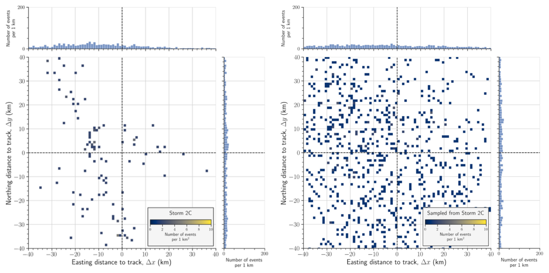
Figure F5 2D spatial count of lightning strokes per 1 km² of easting and northing distances to the movement track in natural time k for thunderstorm 2C (left panel) and for a bivariate Gaussian distribution based on thunderstorm 2C (right panel) for window sizes Δw=500. Only bins with more than 1 lightning stroke are coloured and the plot is zoomed onto [−40, 40] km intervals for both easting and northing distance. The marginal bin counts per 1 km are given for both dimensions.

Appendix G: Sampling, sorting and re-indexing procedure for inter-event time variable

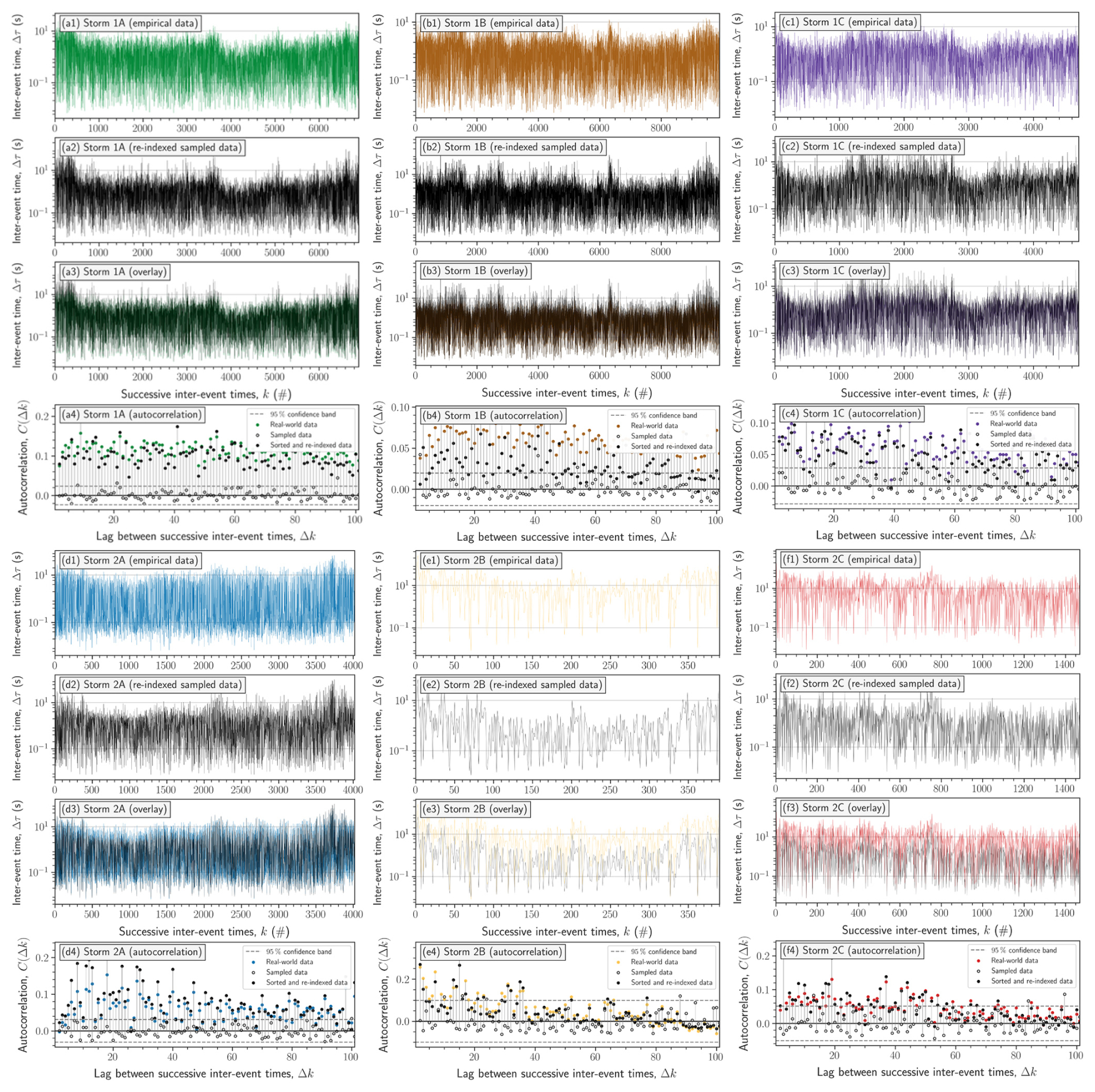
Figure G1 Sampling, sorting and re-indexing procedure based on the combined supercell inter-event time Δτ dataset and thunderstorm (a) 1A, (b) 1B, (c) 1C, (d) 2A, (e) 2B and (f) 2C. The first panel (a1, b1, c1, d1, e1, f1) shows the original cut inter-event time series in natural time k. The second panel (a2, b2, c2, d2, e2, f2) shows this sampled time series being sorted and re-indexed based on the particular thunderstorm, where the indices of the sorted time series coincide between the two time series. The third panel (a3, b3, c3, d3, e3, f3) shows the overlay between the original time-series and the sorted and re-indexed one in natural time k. The fourth panel (a4, b4, c4, d4, e4, f4) show the autocorrelation comparison, including the 95 % confidence band.