Building-level exposure asset value modelling for Germany: an Ahrweiler case study

Verified, harmonised, open-access, object-level exposure data are essential for next-generation risk assessments, risk management, and impact-based forecasting. However, this object-level information is often proprietary, protected by regulation, poorly documented, and fragmented because data on building usage, structural type, or replacement costs are not readily available or not compiled in one dataset. To address this gap, we present an evaluation of exposure model workflows employing various disaggregation approaches and source data from cadastre-derived, crowd-sourced, national accounts, and fit-for-purpose datasets. Using information collected from one flood-affected region in Germany and a weighted scoring model, we evaluate the ability of each workflow to assign a building's economic sector and asset value against our hand-labelled benchmark dataset. Ultimately, we find an exposure model workflow disaggregating national accounts onto cadastre-derived building footprints slightly outperforms the other workflows owing mainly to its transparency and adaptability. However, we conclude that all but the land-use-derived workflow are defensible for object-level exposure modelling – when validated. While these findings are limited to one specific region, the workflows developed here provide the basis for broader evaluation across regions with different building stocks, economic structures, and data quality. Workflows like these enable the transparent, reproducible, and maintainable multi-sector object-level exposure modelling necessary for the next generation of risk analysis and impact forecasting.

1 Introduction

Natural hazards have impacted billions of people globally over recent decades. To mitigate these impacts, communities and governments rely on risk models which provide critical information for risk management (Messner et al., 2007; Merz and Thieken, 2004). These models typically conceptualise risk as arising from the interaction of three components: hazard, vulnerability, and exposure (Crichton, 1999). In this context, exposure refers to the assets at risk from natural hazards, such as buildings, goods, infrastructure, and other elements of value (Merz et al., 2010; Wieland et al., 2015).

Impact forecasting, which predicts the spatially explicit consequences of an imminent event (e.g., the number and location of affected people and buildings, expected damage, or disruption of services), requires detailed exposure and vulnerability information to translate hazards into impacts, thereby motivating object-level (building-scale) exposure models (Apel et al., 2022).

Exposure modelling aims to identify and quantify these assets, focusing on variables related to vulnerability like building size, construction type, construction materials, and asset monetary value (Paprotny et al., 2021; Gerl et al., 2016).

The selection of exposure variables is generally driven by the modelling objectives and availability, underscoring the importance of tailored approaches to risk assessment and impact forecasting.

Empirical studies consistently identify asset monetary value as a key predictor of flood losses (Gerl et al., 2016). This asset value is usually expressed as replacement cost (RC) or depreciated cost (DC). RC denotes the expense of rebuilding with new materials, whereas DC captures age-related depreciation. The perpetual inventory method is commonly used to calculate DC by taking a historic estimate of the building stock (e.g., in Germany by federal state in 1946) and adjusting it annually for new construction, demolition, and other flows to arrive at a net asset value (NAV) (Schmalwasser and Schidlowski, 2006). However, there is no universally agreed framework for these categories, and definitions and methods vary between jurisdictions (see Sect. S1 in the Supplement). Loss modelling has therefore applied RC to estimate total economic exposure or reconstruction needs, DC or NAV for asset accounting and compensation-oriented analyses, and insured value for insurance or reinsurance applications (Daniell, 2014). Market value (the price at which a building can be traded in the marketplace) can be useful for real-estate, relocation, or recovery-planning questions, but appears less often in natural hazard studies (Merz et al., 2010; Gerl et al., 2016; Molinari et al., 2020). For floods, most exposure models still use whole-building asset values, even when the expected damage mechanism is concentrated on the ground or first floor (Gerl et al., 2016; Molinari et al., 2020; Molinari and Scorzini, 2017). Other variables of importance include building volume, often determined by multiplying footprint area (ground contact area) by height, gross floor area (total area of all storeys, excluding the roof), and usable floor area (space available for use, excluding walls) (Zschiesche, 2021).

Traditional hazard exposure models often rely on aggregated approaches, resolving exposed assets at coarse spatial scales such as community-, block-, or grid-level units (Hall et al., 2005; Sairam et al., 2021). These aggregated approaches have been useful in large-scale analysis, but may not provide the accuracy required to support local risk management (Röthlisberger et al., 2018; Bryant et al., 2023; Sieg and Thieken, 2022).

Drawing on local case studies, Wünsch et al. (2009) and Molinari and Scorzini (2017) show that, although the procedure for estimating exposed assets (e.g., binary vs. regression-based asset value disaggregation) influences modelled losses, the spatial resolution of the asset data has an even greater influence.

In contrast to aggregated approaches, object-level exposure modelling evaluates individual assets explicitly, such as the value of single buildings, offering finer granularity or resolution and potentially greater accuracy in damage assessments (Röthlisberger et al., 2018). The potential for this higher resolution to improve accuracy in loss modelling is a function of the spatial variability or spatial correlations of the hazards and vulnerabilities considered.

For example, flood intensities and vulnerability characteristics (e.g., building height) can vary over short distances (e.g., between buildings and streets), making flood exposure models particularly sensitive to resolution (Thieken et al., 2006; Bryant et al., 2023, 2025).

Similarly, tsunami inundation intensities exhibit short spatial correlation lengths, whereas seismic ground motion remains strongly correlated over much larger distances (Gomez-Zapata et al., 2021). Consequently, building-level exposure is considered more important for tsunami loss models, while sub-kilometre-scale resolution may be more reasonable for earthquake loss models (Dabbeek et al., 2021).

The major challenge facing object-level exposure modelling is that available data, like census information aggregated to administrative units, is often coarse and poorly aligned with hazard data. To address this spatial mismatch, regional statistics can be disaggregated into finer spatial units using ancillary data like land use, population, or nighttime lights (Wu et al., 2018; Gómez Zapata et al., 2022). These methods have been applied at local (Custer and Nishijima, 2018; Figueiredo and Martina, 2016; Sieg and Thieken, 2022; Wu et al., 2019), regional (Wünsch et al., 2009), national (Kleist et al., 2006; Röthlisberger et al., 2018; Thieken et al., 2006; Wu et al., 2018), and continental scales (Paprotny et al., 2020a, b; Paprotny and Mengel, 2023; Dabbeek et al., 2021).

For example, Figueiredo and Martina (2016) utilised open building data and census data to disaggregate residential floor area onto a 50 m gridded exposure model to show that coarse exposure models overestimate losses. Similarly, Bryant et al. (2025) used a global flood model to demonstrate the influence of aggregating exposed assets in loss models, showing how typically concave non-linear flood damage functions lead aggregated models to overestimate. Although these and most related studies focus on loss modelling rather than exposure modelling alone, many of their findings translate directly because not only is exposure modelling embedded within the broader loss-modelling workflow, it is also a precondition for it.

Many asset-scale exposure models treat building geometry (i.e., floor area or building volume) as a final multiplier, applied transparently to scale a unit cost (e.g., EUR m⁻² or EUR m⁻³) to obtain asset value (EUR). For example, Paprotny et al. (2020b) disaggregated national gross fixed asset values of dwellings for 22 European Union (EU) countries to derive national EUR m⁻² averages from floor area estimates. Similarly, using public census data, expert knowledge, and engineering manuals, the European Seismic Risk Model 2020 (ESRM20) provides an open-source continental-scale exposure model that estimates occupancy types and typical per-asset-type replacement costs from country-wide unit costs (EUR m⁻²) (see Table S8) (Crowley et al., 2021). Building on the ESRM20 exposure model, Nievas et al. (2023) developed the European High-Resolution Exposure (EHRE) model, which assigns probabilistic ESRM20 building classes to OpenStreetMap (OSM) (OpenStreetMap contributors, 2017) building footprints, while retaining the ESRM20 per-asset-type replacement costs.

Despite recent advancements in disaggregation and exposure modelling, few attempts at validation or comparison have been published (Röthlisberger et al., 2018; Sieg et al., 2023; Sieg and Thieken, 2022; Thieken et al., 2006; Wünsch et al., 2009). Validating against loss records, Schröter et al. (2018) compare cadastre-derived predictors against post-event survey loss models and conventional depth–damage curves to show that these predictors enable object-level loss estimates with accuracy comparable to survey-based models and substantially better than depth–damage curves. However, we are aware of no published direct comparison or validation of locally explicit building asset values. To address these gaps, our study aims to develop and compare several exposure model workflows for object-level exposure estimations applicable to Germany. Specifically, the objectives are to survey and identify potential data sources, design a set of candidate workflows, and quantitatively evaluate these while deliberately retaining their different source cost bases (RC, DC, and NAV) for transparency, to identify a robust, reproducible workflow for multi-sector risk analysis and impact forecasting.

2 Methods

Our study first developed and processed candidate sector classification and asset value workflows, fundamental components of exposure models. These workflows were then evaluated using a hand-labelled benchmark dataset we built for our study area.

2.1 Study Area

Our study focuses on the Ahrweiler District (“Landkreis Ahrweiler”) in western Germany (Fig. 1). In July 2021, the region experienced a severe flood event that caused significant economic losses and fatalities (Lehmkuhl et al., 2022) (see Fig. 2). Ahrweiler’s history of flooding spans centuries, with over 70 floods recorded in the past 500 years (Brühl, 2025), the first one being reported in 1348 (Seel, 2025).

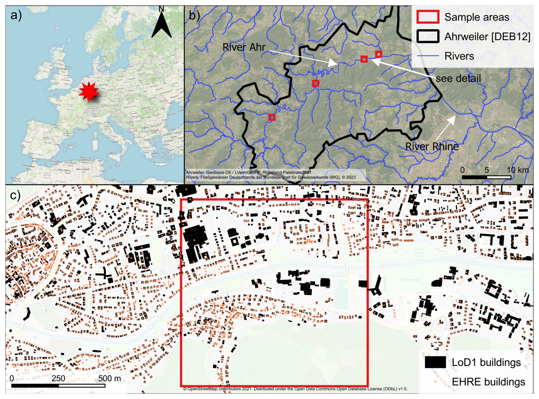
Figure 1 Study area maps showing: (a) study location; (b) study boundary (Nomenclature of Territorial Units for Statistics level 3 [NUTS 3] name [and code]); and (c) typical detail of village area with building locations from datasets discussed in the text. Map data from OpenStreetMap, licensed under the Open Database License (ODbL) – https://www.openstreetmap.org/copyright (last access: 31 August 2026).

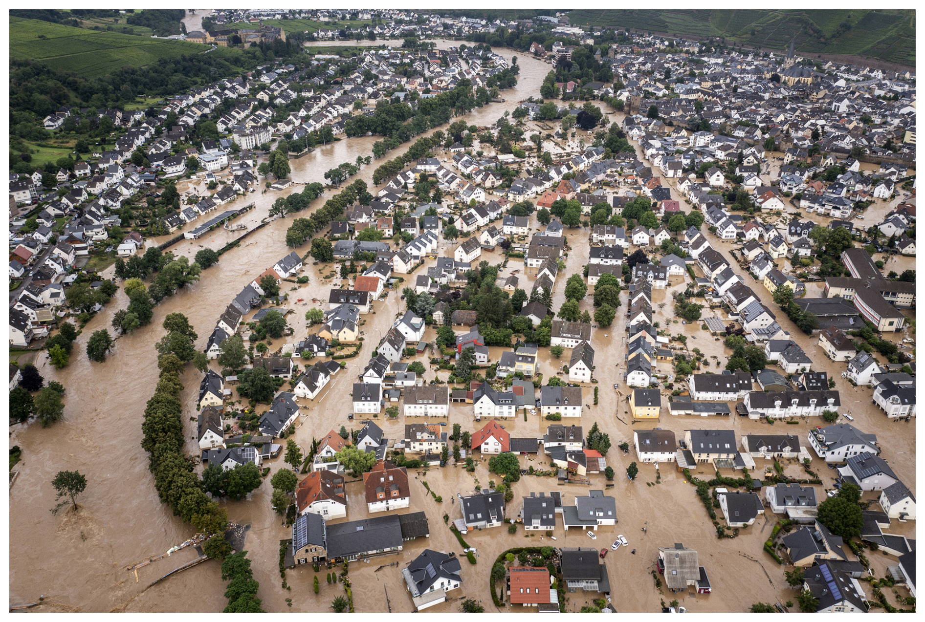
Figure 2 Overview of typical buildings during the 2021 floods. Image © Christian/Adobe Stock (ID: 447651476), licensed by GFZ Helmholtz Centre for Geosciences Potsdam.

The service sector dominates Ahrweiler's economy, accounting for 70.9 % of gross domestic product (GDP), followed by manufacturing industry (27.8 %) and agriculture, forestry, and fishing (1.2 %) (Statistisches Landesamt Rheinland-Pfalz, 2025). Land use is 53.3 % forest and vegetation, 31.1 % agriculture, 7.2 % settlements (3.3 % residential, 1.0 % industrial, 1.6 % recreational), 6.8 % infrastructure, and the remainder water bodies and other uses (Statistisches Landesamt Rheinland-Pfalz, 2025). Public records show over 40 000 residential buildings with 88.8 % being detached and semi-detached houses (as of 2023) and roughly 6000 registered companies (Statistisches Landesamt Rheinland-Pfalz, 2025).

2.2 Data

To develop and process our candidate exposure model workflows, we began by searching for freely available building-exposure and asset-value datasets, with a focus on building fixed asset values (i.e., values for structural and non-structural architectural components of the buildings rather than movable contents/equipment). A systematic search using Google (Google, 2025a) and Google Scholar (Google, 2025b) yielded the datasets summarised in Table S2, from which we then selected those datasets listed in Table 1 for further analysis (see Sect. S2 for details).

Eurostat (2025b)Eurostat (2025a)Insee (2022)Paprotny (2022)Copernicus (2020)Nievas et al. (2023)BKG (2023)OpenStreetMap contributors (2017)Copernicus Land Monitoring Service (2018)BKG (2024)BKI (2021)

Table 1 Summary of datasets and sources used in this study. CORINE: Coordination of Information on the Environment; DC: depreciated cost; NAV: net asset value; NUTS: Nomenclature of Territorial Units for Statistics; RC: replacement cost; n/a: not applicable.

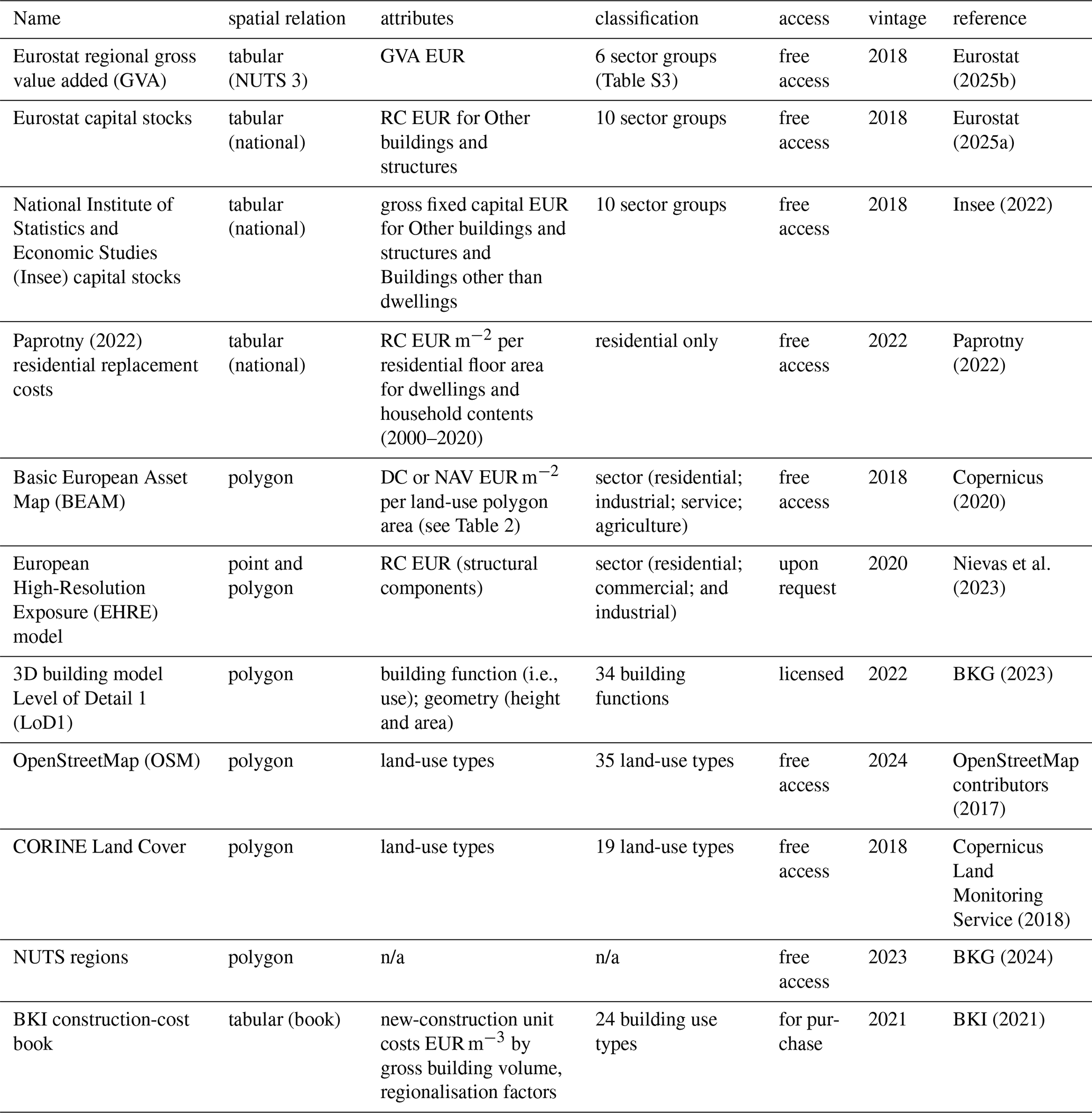
The three asset value candidate datasets considered here are the Basic European Asset Map (BEAM), EHRE, and data derived from the European Statistical Office (Eurostat). While the raw EHRE data is object-level and model-ready, the BEAM and Eurostat data require additional processing with ancillary data as described in the following sections.

2.2.1 Datasets from the Statistical Office of the European Union (Eurostat)

The Statistical Office of the European Union (Eurostat) provides harmonised economic data across member states, making it an invaluable source for national-level asset value estimates (Eurostat, 2013). In Germany, state statistical offices collect these data, and “Statistisches Bundesamt (Destatis)” (Federal Statistical Office) organises the national submission to Eurostat (Arbeitskreis Volkswirtschaftliche Gesamtrechnungen der Länder, 2021). Prior to 2025, data were usually organised using the Statistical Classification of Economic Activities in the European Community (NACE Rev. 2), a hierarchical scheme distinguishing 21 level-one categories or sectors (European Commission, 2008).

For example, the GVA at basic prices by NUTS 3 region table (Eurostat, 2025b) provides an estimate for the economic output minus consumption by allocating national totals to regions, using as much regional data as possible while maintaining consistency with national totals (European Commission. Statistical Office of the European Union, 2013). This table provides GVA estimates per year for NUTS 3 regions (roughly 400 in Germany) for six economic sector groups (see Table S3).

Providing a more refined discretisation by asset types, the Capital stocks by industry (NACE Rev. 2) and detailed asset type table (Eurostat, 2025a) estimates the value of fixed assets per year at national scale for 21 NACE (level-one) sectors.

Values are provided on a gross or net basis; gross denotes the value of all fixed assets still in use valued at current replacement cost (as if new), whereas net deducts accumulated consumption of fixed capital.

The table provides gross values for the asset category Other buildings and structures (AN.112) which is an aggregate of the categories shown in Table S4. Therefore, the published AN.112 category lumps together many assets not of interest to exposure modelling of non-residential building assets (e.g., railways), and generally requires some disaggregation (e.g., to AN.1121) if used as such (Paprotny et al., 2020a).

2.2.2 Basic European Asset Map (BEAM)

BEAM was developed to “estimate, evaluate and compare real and potential damages caused by natural disasters all across Europe” and provides 11 asset layers using the “net concept, which reflects the depreciated construction costs (not restoration costs or insured assets)” (Copernicus, 2020). These values are provided as NUTS 2-level EUR m⁻² averages per land-use area, not per building area, then mapped to land-use polygons so that obtaining per-building asset values requires aggregating polygon totals and redistributing them to individual buildings. From these 11 layers, we focus here on those related to building asset values listed in Table 2. For residential buildings, BEAM estimates DC by multiplying EUR m⁻² construction costs by a depreciation rate, before disaggregating to land-use polygons with regional unit counts and density factors. In contrast, for non-residential buildings, BEAM estimates NAV by allocating national totals to NUTS 2 regions before disaggregating to land-use polygons using employee counts and density factors.

Table 2 BEAM asset layers (Copernicus, 2020) included in our study. Note that for our analysis, asset values are multiplied by the factors shown in Table S7 to isolate the “building” portion (see text for details). DC: depreciated (construction) cost; NAV: net asset value.

While the BEAM data product is freely available and its methods are (briefly) summarised in IABG mbH and geomer GmbH (2020), all factors mentioned above and the software pipeline are unpublished and proprietary. We use the 2020 “Germany BEAM update”, as the 2025 release appeared while this article was in review (IABG mbH and geomer GmbH, 2025). Although the cost bases and four relevant asset categories remain the same, we expect these updated national-account values, finer land-use data, revised settlement-density factors, etc., would materially change the numerical results, without affecting our description of the BEAM methodology or conclusions.

2.2.3 European High-Resolution Exposure (EHRE) model

The EHRE model presented in Nievas et al. (2023) is a Europe-wide exposure model that results from the combination of (i) the aggregated exposure model of ESRM20 (Crowley et al., 2020, 2021), (ii) data on individual buildings from OSM, processed as OpenBuildingMap (OBM) (GFZ Helmholtz Centre for Geosciences, 2024; Schorlemmer et al., 2020, later developed and enriched with other datasets by Oostwegel et al., 2025), and (iii) remote sensing-derived built-up areas from the Global Human Settlement Layer (GHSL) (Corbane et al., 2018). It represents buildings as a combination of individual OSM building footprints and, in regions where OSM is deemed incomplete, remainder estimates, which are represented on a ≈100 m grid. EHRE inherits all the occupancy cases, structural classes (Global Earthquake Model [GEM] Building Taxonomy v3.0, Silva et al., 2022), number of building occupants, and per-asset-type replacement costs from the ESRM20 model. For Germany, these estimates are based on census data retrieved in 2011 (Crowley et al., 2020). Individual building footprints are assigned by EHRE a series of potential structural classes and their associated probabilities.

ESRM20 RC, referenced to 2020, is obtained by applying country- and occupancy-specific reconstruction costs (EUR m⁻², see Table S8), adjusted by material-dependent modifiers (0.95–1.05) which are then multiplied by the average usable floor area of each building class in a region. In EHRE, these regional values are maintained and object-distributed, not adjusting for the geometry (i.e., area) of OBM buildings. In other words, ESRM20 estimates regional exposure on administrative units (totals and averages), whereas EHRE distributes these values to the building scale by linking ESRM20 classes and costs to individual OSM footprints (and filling gaps with aggregated remainder buildings).

EHRE inherits the occupancy types of individual OSM footprints from OBM, which assigns them by: (i) retrieval of all OSM tags associated with the building, (ii) mapping of the OSM tags onto the 53 GEM Taxonomy occupancy types, and (iii) a final rule-based selection. EHRE then groups these 53 GEM occupancy types into three modelled occupancy cases – residential (14 types), commercial (6 types), and industrial (6 types) – and treats the remaining 27 as other types outside the ESRM20 building-class set, with no replacement value assigned. EHRE's consolidation requires deterministic allocation of some mixed-use (MIX) categories to modelled occupancy cases; for clarity, the full mapping is reproduced in Supplement Data Table 1.

Extracts of the EHRE model are available upon request, and the whole suite of software used to create it is publicly available and open-source (see Nievas et al., 2023 for details).

2.2.4 Ancillary datasets

The Level of Detail 1 (LoD1) dataset provided by the Bundesamt für Kartographie und Geodäsie (BKG) (“Federal Agency for Cartography and Geodesy”) (BKG, 2023) provides information on buildings across Germany. It includes polygons of all buildings that are recorded in the Amtliche Liegenschaftskatasterinformationssystem (ALKIS) (“Official Real Estate Cadastre Information System”) of all German federal states (AdV, 2023) as of 2022. LoD1 is cadastre-derived, drawing directly on authoritative land parcel and building records maintained by state cadastral offices, ensuring national coverage, legal consistency, and administrative validity. Information on individual building use types (called “[building] function”) is given for each individual building as well as the building height. In the LoD1 dataset, roof shapes are assumed to be flat; consequently, heights of complex buildings are averaged. LoD1 building use or function is recorded by the cadastral authorities of the federal states, based on information such as building permit applications (Waldhof, 2025). For the analysis below, geometries with non-building functions (e.g. stadiums, water tanks, bridges) were discarded.

Another source we use for building data is OSM (OpenStreetMap contributors, 2017), a global editable map database built and maintained by volunteers. It describes a large number of geographic features, including individual building footprints, roads and land-use polygons, providing 35 land-use classes in our study area.

Further land-use information was obtained from Coordination of Information on the Environment (CORINE) Land Cover data (Copernicus Land Monitoring Service, 2018) which includes a pan-European land-cover and land-use inventory with 44 classes, 19 of which are found in our study area.

Benchmark construction cost information was sourced from Baukosten Gebäude Neubau 2021 (BKI) (“Construction costs for new buildings 2021”) (BKI, 2021). BKI (2021) provides construction cost values of 75 different building use types as EUR m⁻³ (see Table S9), based on a database of several thousand invoiced projects for new buildings collected by architectural associations in Germany. These unit costs refer to gross building volume (Bruttorauminhalt, BRI), which is derived from gross floor area by storey, measured to the outside of external walls, and the vertical distance between floor or ceiling reference surfaces, with roof volumes treated according to roof geometry (Zschiesche, 2021). This book, published by BKI (2021), is available for purchase online for personal use and is intended to provide a realistic basis for reliable cost estimation of construction projects for architects, engineers, and building contractors.

2.3 Candidate Workflows

In natural hazards research, the variables selected for exposure models are typically guided by vulnerability research and the availability of data. This commonly leads building-related models to include categorical dimensions such as use, construction type, and economic sector. These categories provide informative predictors of vulnerability behaviour (e.g., via stratified modelling) and, in the case of economic sector classification, useful dimensions for communicating results to stakeholders. In practice, sector classification (e.g., residential, industrial, service) is frequently applied deterministically to each asset by transferring labels from a related, more granular categorical source (e.g., building function or land use) with a simple lookup table or reclassification schema. While there is no standard sector classification label set for building use, common frameworks include NACE 2.0 with its 21 economic areas (see Table S3) or a more basic framework like the one employed by BEAM (Table 2).

Here, we adapt or develop the workflows for assigning sector labels to building assets shown in Table 3, and evaluate these against our hand-labelled benchmark dataset.

(Paprotny et al., 2020a)(Paprotny et al., 2020b)(Copernicus, 2020)(Nievas et al., 2023)(BKI, 2021)

Table 3 Method summary of study exposure model workflows and benchmark dataset. n/a: not applicable.

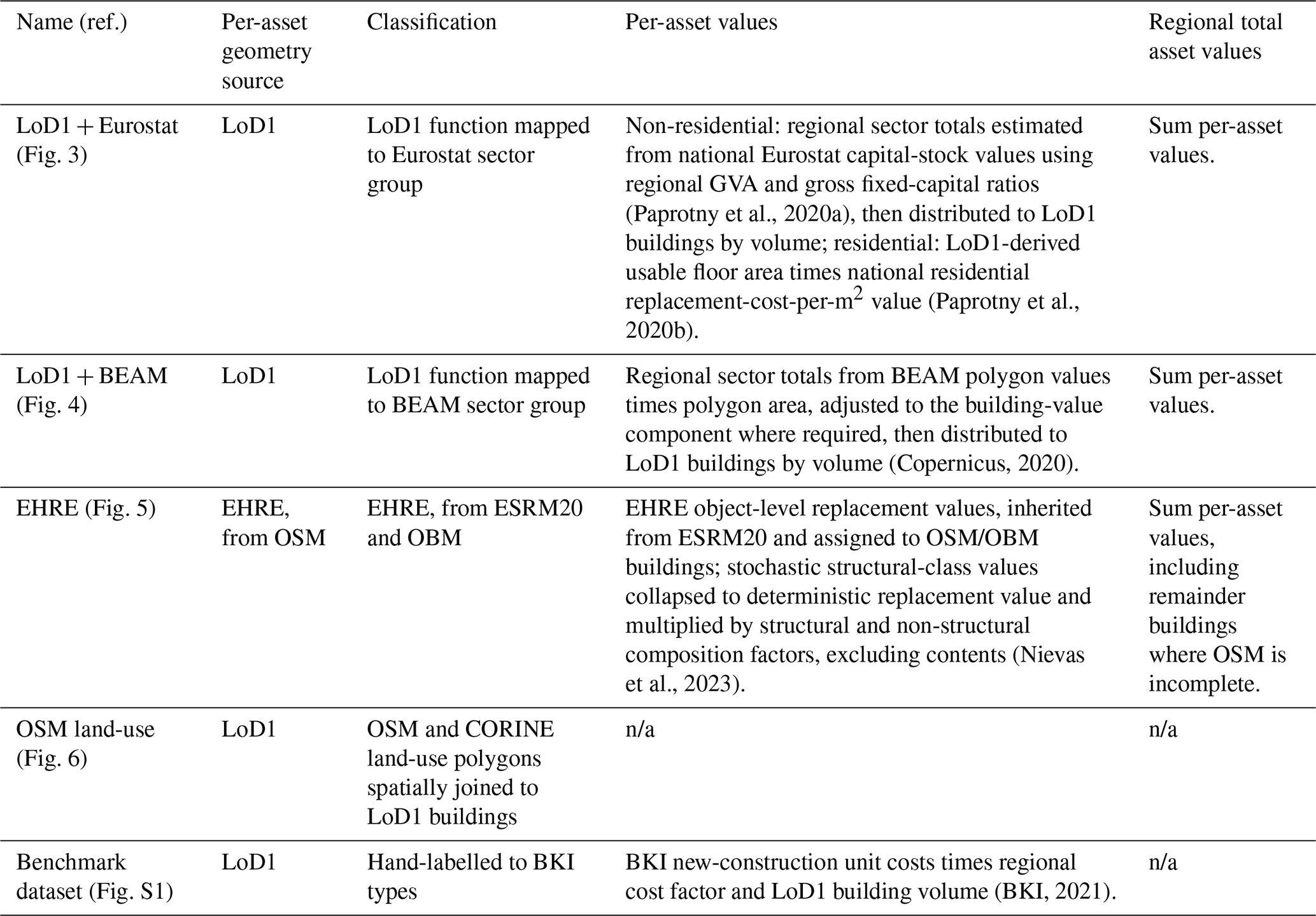
From these, the three best-performing workflows are further developed into asset value workflows formulated on BEAM, Eurostat, and EHRE datasets as described below. All resulting derived datasets are provided in Buhrmann (2025a, b).

2.3.1 LoD1 + Eurostat

The first workflow we consider uses the granular per-asset building function information obtained from the LoD1 dataset and a reclassification schema (Supplement Data Table 1) to map these to the six sectors provided by Eurostat (2025b) (see Table S3).

To obtain asset-value estimates from this per-asset sector-classified layer, we adopted the method of Paprotny et al. (2020a) for non-residential and Paprotny et al. (2020b) for residential RC as shown in Fig. 3.

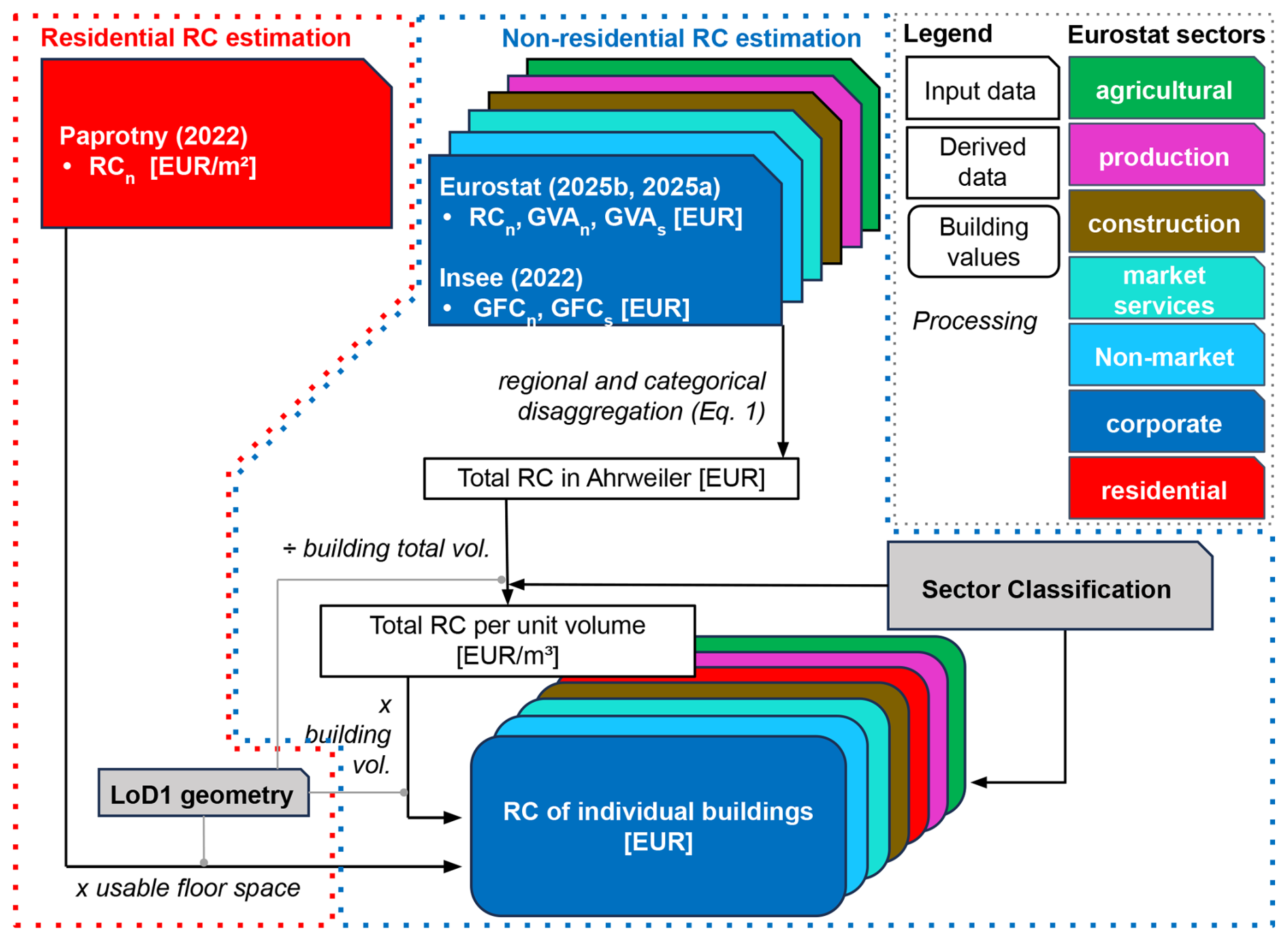
Figure 3 LoD1 + Eurostat asset value model workflow adapted from Paprotny et al. (2020a, b) showing the residential (red) and non-residential (blue) RC calculation.

Accordingly, to obtain an estimate per-sector of the regional RC for non-residential buildings for our year of interest from published data, Paprotny et al. (2020a) disaggregates both spatially (national to regional) and categorically (AN.112 to AN.1121). These disaggregations are achieved using simple ratios obtained from ancillary data tables:

$$\begin{array}{}\text{(1)}& \begin{array}{rl}{\mathrm{RC}}_{r,s,y,\text{AN.1121}}={\mathrm{RC}}_{n,s,y,\text{AN.112}}& \times {\displaystyle \frac{{\mathrm{GVA}}_{r,s,y}}{{\mathrm{GVA}}_{n,s,y}}}\\ & \times {\displaystyle \frac{{\mathrm{GFC}}_{n,s,y,\text{AN.1121}}}{{\mathrm{GFC}}_{n,s,y,\text{AN.112}}}}\end{array}\end{array}$$

where RC${}_{r,s,y,\text{AN.1121}}$ is the Buildings other than dwellings (AN.1121; Table S4) RC for a NUTS 3 region r in sector s for year y; RC${}_{n,s,y,\text{AN.112}}$ is the national gross RC for Other buildings and structures (AN.112) assets from Eurostat (2025a); GVA${}_{n,s,y}$ is the national and GVA${}_{r,s,y}$ is the NUTS 3 regional GVA from Eurostat (2025b); and ${\mathrm{GFC}}_{n,s,y,\text{AN.112}}$ and ${\mathrm{GFC}}_{n,s,y,\text{AN.1121}}$ are the gross fixed capital for Other buildings and structures (AN.112) and Buildings other than dwellings (AN.1121) respectively obtained from Insee (2022) (Paprotny, 2025). Values for each variable are provided per-sector group in Tables S5 and S6.

Within our NUTS 3 region, these values were finally distributed to individual buildings proportional to building volume (m³), computed by multiplying LoD1 footprint area by height attributes.

For residential buildings, asset values were calculated as usable floor area multiplied by the national replacement cost of EUR 2478 m⁻² from Paprotny (2022). Paprotny et al. (2020b) derived this unit cost by dividing the national gross replacement cost of the dwelling stock, estimated from Eurostat national accounts and 2018 perpetual-inventory estimates, by the total residential floor area in Germany. Usable floor area was estimated by multiplying LoD1 footprint area by storey count and a 0.7 usable-area coefficient, with storeys inferred from LoD1 height using 3.3 m for the ground floor and 2.4 m for each additional storey (Figueiredo and Martina, 2016; Paprotny et al., 2020b). The resulting footprint-to-usable-area relation for all residential buildings is shown in Fig. S4.

2.3.2 LoD1 + BEAM

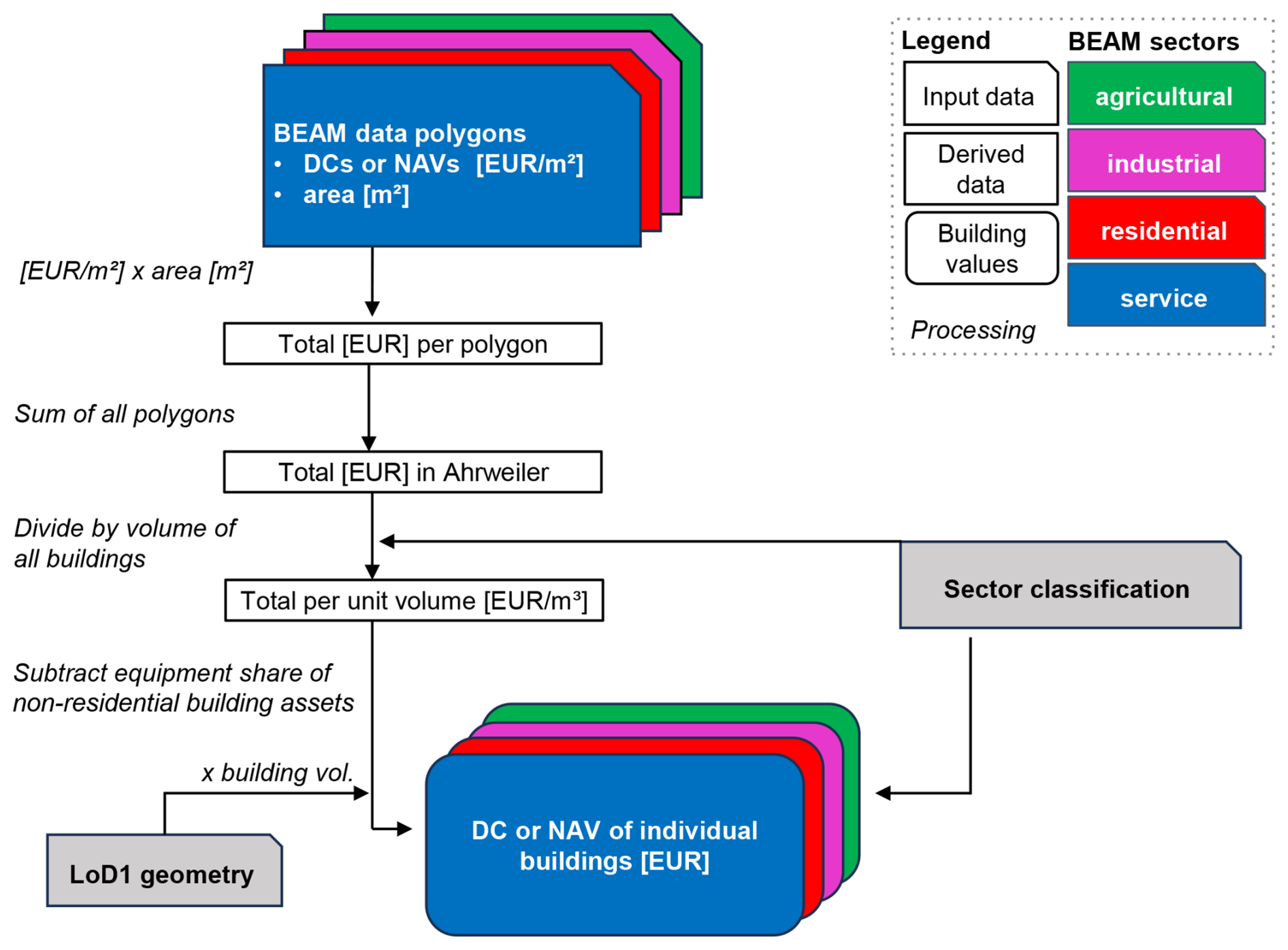
The second workflow considered here provides a similar classification based on LoD1 function data, but using disaggregated BEAM data for asset values. Accordingly, a separate reclassification schema was used to map the LoD1 function values to one of the four sectors: residential, industrial, service, or agriculture (Supplement Data Table 1).

As the BEAM dataset provides a relatively coarse land-use-polygon-scale EUR m⁻² asset value, and here we focus on per-asset values, we opted to back-calculate a regional aggregate EUR, then redistribute this to individual buildings by volume for each sector.

For all non-residential sectors, it was necessary to subtract the equipment values included in BEAM from our building value estimate, for which per-sector multipliers adapted from Arbeitskreis Volkswirtschaftliche Gesamtrechnungen der Länder (2023) and shown in Table S7 were used.

See Fig. 4 for a visualisation of the workflow.

Figure 4 LoD1 + BEAM asset value model workflow.

2.3.3 EHRE

For the residential, commercial, and industrial buildings, EHRE links each footprint to stochastic structural classes and ESRM20 per-asset-type replacement values. To obtain a single deterministic building asset value for comparison against the other workflows, we sum and collapse these classes to a single weighted-mean replacement value, then multiply by the structural and non-structural factors shown in Table S8 (effectively excluding the “contents” component).

The EHRE workflow is visualised in Fig. 5 and the source EHRE data extract is provided in Nievas (2025).

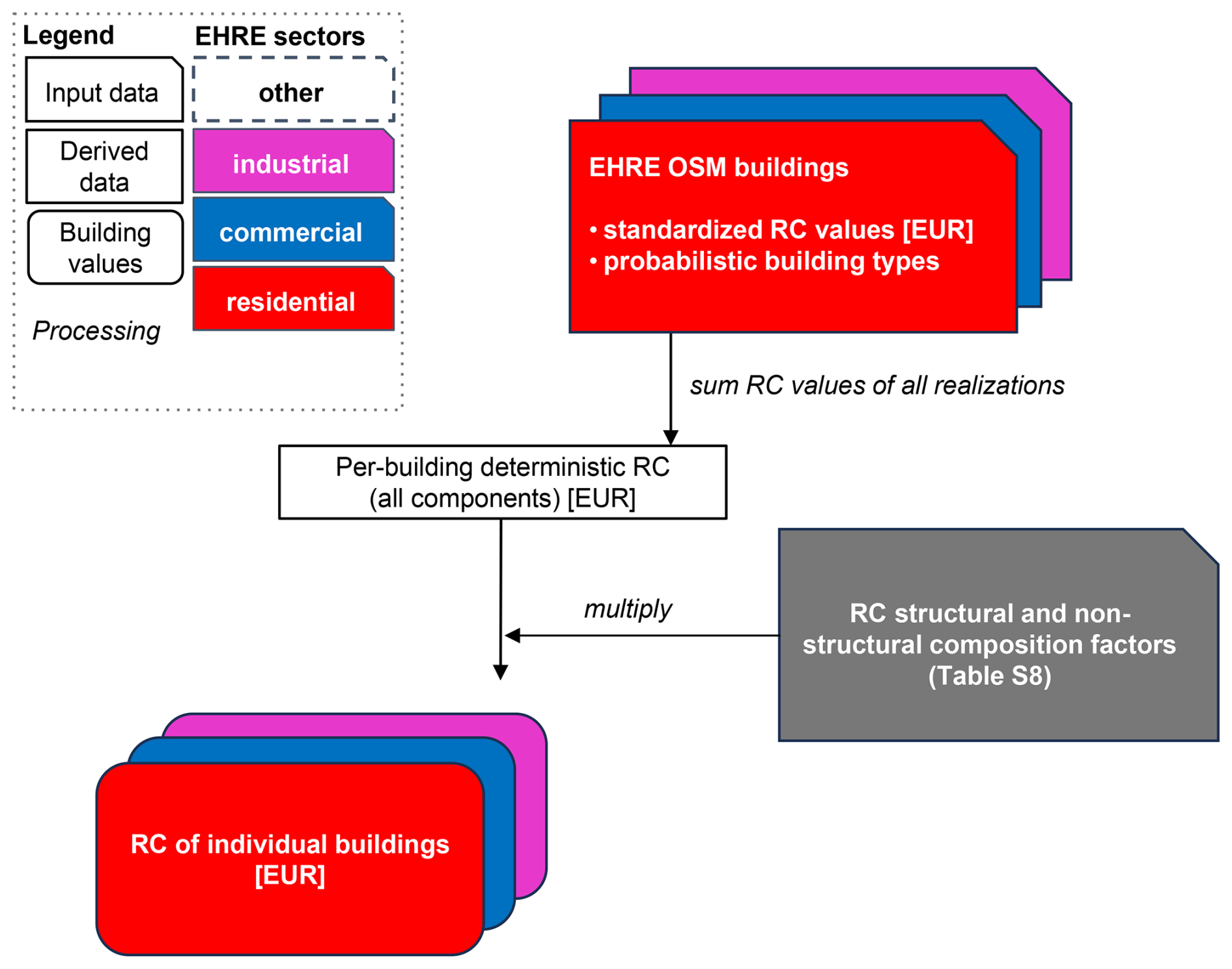
Figure 5 EHRE asset value workflow adapted from Nievas et al. (2023). Note other category assets do not contain asset values and are therefore omitted from value calculations.

2.3.4 OSM land-use classification

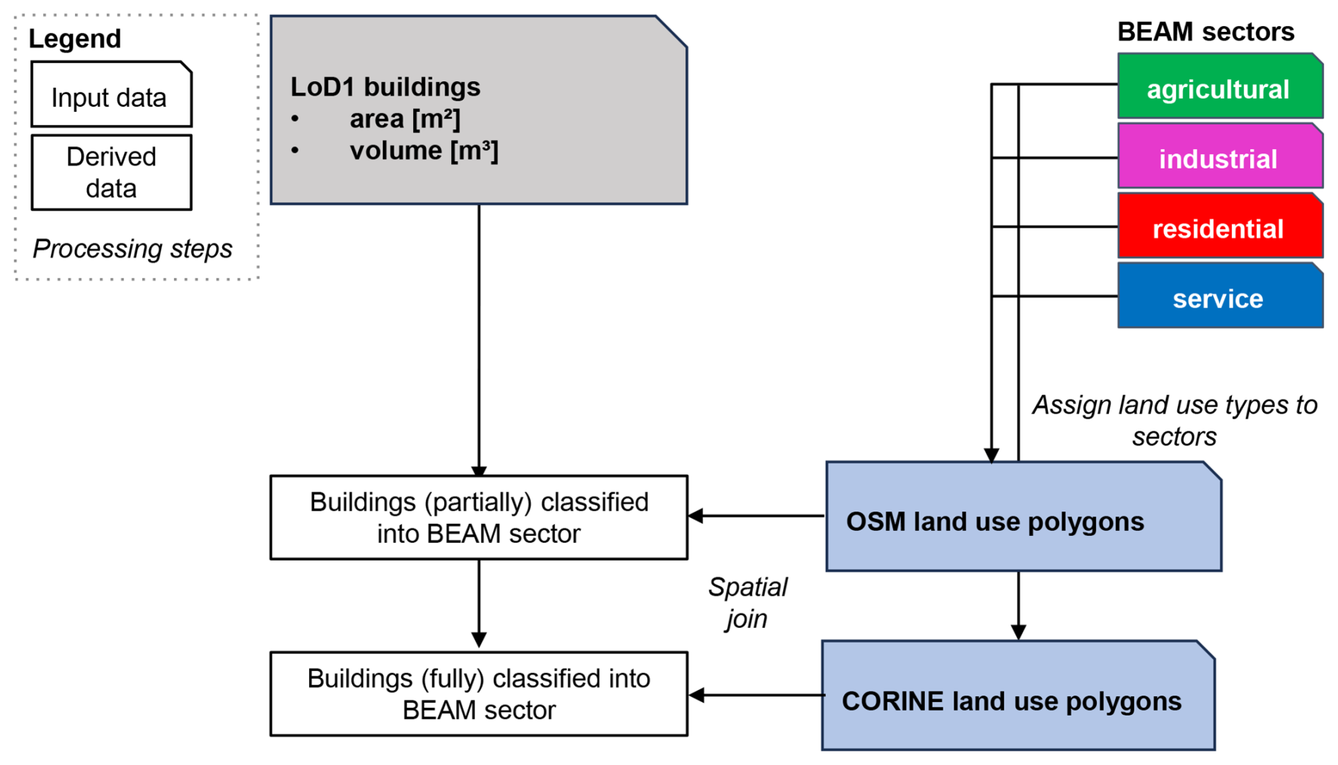
For comparison against the building-attribute-based sector classification model workflows above, we developed an alternative classification approach based solely on open-source land-use data, hierarchically prioritising the more granular OSM polygons over CORINE gridded land-use data. First, the land-use classes of both datasets were classified into one of BEAM's economic sectors using the lookup table from Supplement Data Table 1 before spatially joining onto LoD1 building locations. This results in most assets (96.73 %) sourcing land-use information from the OSM polygons, but in some areas where these are missing the CORINE value is taken. The land-use-based workflow is shown in Fig. 6.

Figure 6 OSM land-use sector classification model workflow.

2.4 Benchmark Dataset

To develop our benchmark dataset, we selected four representative study plots based on knowledge of the region (Fig. 1). From these, a dataset of 844 sample buildings focusing on the four study plots and the village of Bad Neuenahr-Ahrweiler was created by hand (based on LoD1 geometries) representing typical residential and non-residential buildings in Ahrweiler (Buhrmann, 2025b).

Assets were classified into 24 building use types from BKI (2021), which we further categorised into the three basic sectors residential, industrial, and service and a fourth ambiguous category as a catch-all for building use types (e.g., “commercial buildings, with apartments”, “Warehouse/storage building, single-use”) whose sector assignment does not neatly fit into the three basic sectors (see Supplement Data Table 1 for complete specification of the sector label mapping). Building classifications were determined through detailed visual inspections using Google Earth (Google, 2024a), Google Street View (Google, 2024b), Mapillary (Meta Platforms Ireland Limited, 2024), and ImmoScout24 (Immobilien Scout GmbH, 2024) in March 2024, comparing 3D representations to descriptions and images in BKI (2021) and site visits (see Sect. S4 for details). Unit construction costs from BKI (2021) ranged from EUR 370–495 m⁻³ for residential, EUR 210–290 m⁻³ for industrial, EUR 215–545 m⁻³ for service, and EUR 160–495 m⁻³ for ambiguous building use types (Table S9). New construction costs per-asset were then calculated by multiplying the relevant unit construction cost, the regional cost factor for Ahrweiler county (0.986; also provided in BKI, 2021), and individual building volumes from LoD1.

The benchmark dataset creation is summarised in Fig. S1.

3 Results and Discussion

This section presents and discusses the results along three dimensions: sector classification, regional total asset values, per-asset values, and finally a semi-quantitative scoring of the candidate workflows.

3.1 Sector Classification

To quantify the classification performance, we first calculated one-vs.-rest confusion counts and derived precision, recall, and F1 for each benchmark dataset sector and each workflow (Sect. S5). The differences in classification results between the four workflows against the four sectors of the benchmark dataset for the 844 sample buildings are summarised in Fig. 7 with per-label performance metrics provided in Table S11 and mean values for each workflow in Table S12.

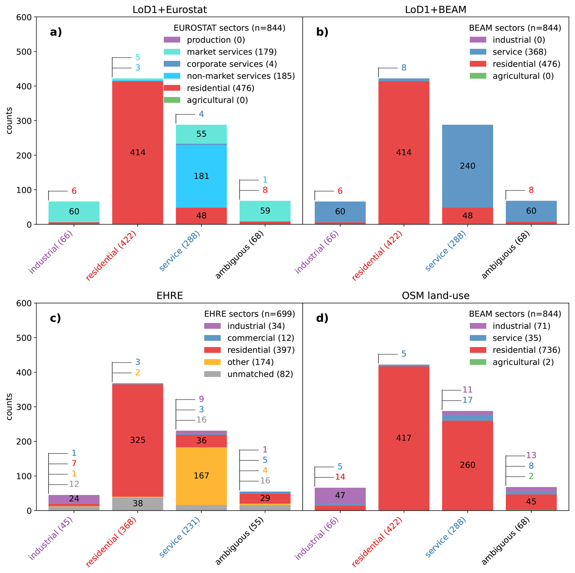
Figure 7 Sample building sector classification results against the benchmark dataset for four workflows. Bars labelled by building count and grouped by the three economic sectors of the benchmark dataset plus a fourth ambiguous category. Bars are coloured by the sector classification of each workflow. Note that no Eurostat production and no BEAM industrial features are among the 844 sample buildings (unlike in the whole case study area). Also note that EHRE (panel c) is natively OSM-indexed (unlike the others which are LoD1 indexed), leading to unmatched records (n=82); other panels had no unmatched records as they share the geometry indexing of the benchmark dataset. EHRE also treats some benchmark dataset building collections as single-part, leading to the anomalous total building count (n=699) (see text for details).

Across the four workflows, precision ranges from 0.50–0.66, recall from 0.57–0.78, and the F1 score (F1) from 0.45–0.71 (Table S12), with LoD1 + Eurostat (Fig. 7a) and LoD1 + BEAM (Fig. 7b) performing best (F1 = 0.71).

Both these workflows are in perfect agreement with each other (assuming equivalence of all Eurostat services labels per Table S10) as both share a LoD1 “function” basis and vary only in their terminal category assignments (see Supplement Data Table 1). This LoD1 data assigns roughly 75 % of the non-residential buildings in our benchmark dataset to “Building for business or trade” which we map to market services and service in the Eurostat and BEAM workflows respectively. However, our manual classification of these buildings in the benchmark dataset describes many as industrial (n=66) or ambiguous (n=68). In other words, while some rare buildings with specific uses are well classified in LoD1 (e.g., schools, churches, fire departments), there is insufficient resolution (i.e., label groups are too broad) to differentiate between the more numerous industrial and service buildings. Beyond this, the two additional categories in the Eurostat workflow compared to the BEAM workflow (six vs. four) give Eurostat slightly more resolution. The utility of this can be seen in the non-market services category (Fig. 7a), 97 % of which match the benchmark dataset service classification. However, because we opted for a simple four-category benchmark dataset, this advantage is not reflected in the performance metrics of Table S12.

The OSM land-use workflow (Fig. 7d) performs the worst of all workflows (F1 = 0.45), chiefly by over-assigning buildings to the residential sector. For example, about 90 % of buildings labelled as service in the benchmark dataset are misclassified as residential by this workflow. This bias arises from the application of coarse land-use polygons downscaled to individual buildings in dense, predominantly residential areas that contain a small number of service buildings. In such settings, buildings belonging to a minority-sector (e.g., service) are misclassified to the dominant residential land use during the polygon-to-object translation.

To compare against EHRE (Fig. 7c), which is indexed to OSM geometry, it was necessary to spatially join the EHRE records to the LoD1-based benchmark dataset (see Sec. S5).

Because LoD1 is designed for 3D building representation, some objects that are single-part in EHRE are multi-part in LoD1; to provide a fair comparison, we merged these LoD1 building parts (see label “c” in Fig. S2). We also manually shifted <1 % of LoD1 features in obvious near-match cases, but left benchmark dataset records without a plausible EHRE counterpart unmatched. This yielded 617 record matches and 82 orphaned benchmark dataset records, which are likely attributable to differences in data vintage because they exist in LoD1 but not in OSM (see label “b” in Fig. S2). Conversely, EHRE records not present in the benchmark dataset were discarded (see label “d” in Fig. S2).

Considering these disparate geometries, EHRE had comparable performance to the other non-land-use-based workflows in the residential sector (F1 = 0.89).

However, EHRE generally assigned the service sector benchmark dataset labels to the other category, which EHRE uses as a catch-all for buildings whose occupancy type is unknown (because of a lack of OSM tags, or lack of OBM rules to translate those tags into a final occupancy type) and buildings whose OBM occupancy type does not correspond to any of the three ESRM20 occupancy cases (residential, commercial, industrial). We treat EHRE's application of these other labels as omission errors, because replacement values are omitted from these assets, rather than as commission errors, which would imply an active assertion of the wrong label (see label “e” in Fig. S2).

If we were to instead map this other category to service, EHRE's weighted score for this sector would increase enough to surpass the LoD1-based workflows (F1 = 0.85).

Further, as our evaluation only considers asset-to-asset comparisons, we do not consider any of the residential or commercial remainder buildings imputed by the EHRE model (Table 4).

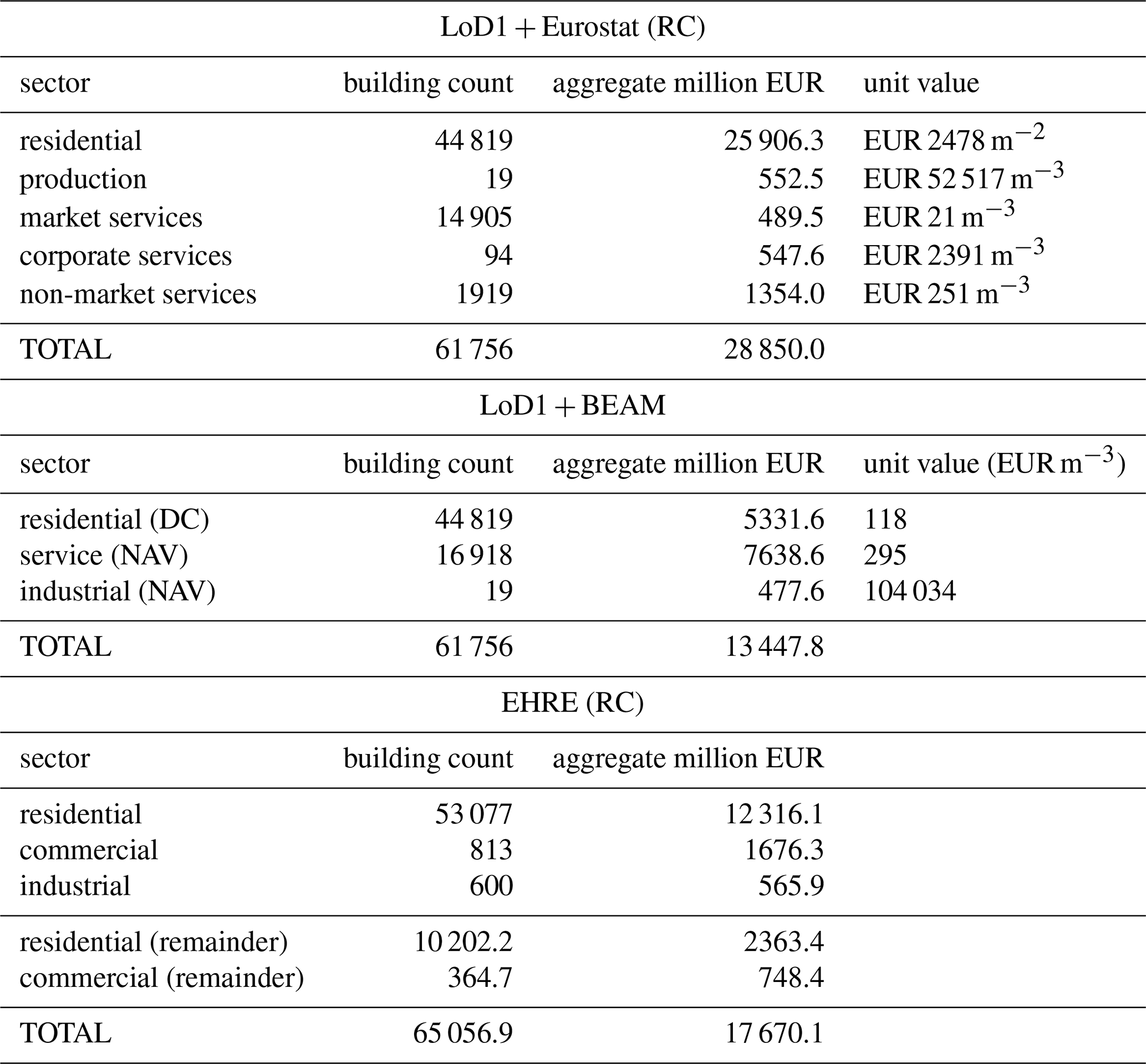
Table 4 Asset-value workflow results per sector for Ahrweiler (DEB12; Fig. 1). Sectors with no buildings are omitted. See text for workflow descriptions. Remainder buildings are a special category provided by the EHRE model that impute missing OSM data which can result in decimal values. NAV: net asset values; RC: replacement costs; DC: depreciated (construction) costs.

The three classification sectors of the benchmark dataset (industrial, residential, and service) show variable performance across the four workflows.

The highest classification agreement was observed for residential buildings, with all workflows classifying nearly all sample buildings consistently (recall ≥0.98); over-assignment of residential labels was more challenging, especially for OSM land-use (Fig. 7d; precision = 0.57) as discussed above.

For the service sector, the LoD1 function-based workflows (Fig. 7a, b) had reasonable true positive capture (recall = 0.83), but over-classified industrial and ambiguous buildings as service (precision = 0.65).

For industrial assets, EHRE performed best (F1 = 0.72), with the OSM land-use workflow close behind (F1 = 0.69), suggesting industrial land use is relatively distinct and well mapped in OSM for our study area. On the other hand, the LoD1-based workflows failed to map any industrial assets owing to the lack of any such labels within our sample building set (see Fig. 7).

The final benchmark dataset category ambiguous was used as a catch-all for unclear or mixed building use in our hand labelling.

As the two LoD1-based workflows (Fig. 7a, b) do not have any mixed or ambiguous categories, these benchmark dataset buildings were forced into standard LoD1 function classes. For example, the benchmark dataset ambiguous class includes labels such as “Commercial buildings, with apartments”, “Warehouse/storage building, single-use”, and “Single, multiple and multi-storey garages”, whereas LoD1 represents buildings through ordinary function labels such as “Building for business or trade”, “Garage”, or “Parking garage” rather than a mixed or ambiguous class.

Similarly, EHRE does not have an ambiguous category because it deterministically maps MIX occupancy types to residential, industrial, or other categories (see Supplement Data Table 1). If these EHRE mixed (MIX) assets were instead mapped to the benchmark ambiguous category, EHRE would yield fewer false positives (precision increasing from 0.56 to 0.60), but with a small loss in recall (0.57 to 0.55) and therefore a negligible improvement overall (F1 increasing from 0.53 to 0.54).

In summary, the LoD1 function-based workflows (Fig. 7a, b), with their government-collected per-asset data (and unfortunate use restrictions) unsurprisingly provided the closest match to our hand-labelled benchmark dataset, despite being unable to identify any industrial or ambiguous buildings. The open-source object-based EHRE also performed well (Fig. 7c), especially if the other category were considered service and the MIX category were considered ambiguous. Lastly, the open-source hierarchical imputation OSM land-use-based workflow (Fig. 7d) performed the worst against our benchmark dataset, primarily through the over-assignment of residential labels; therefore, we exclude this workflow from the subsequent sections. Including it in the regional-total and per-asset value comparisons would require joining the OSM labels to an asset-value source such as Eurostat, producing an OSM + Eurostat hybrid that would mix label performance with the same Eurostat value basis already represented by LoD1 + Eurostat. This would add redundancy and confusion rather than new asset-value information, while EHRE already provides an OSM-based asset estimate.

3.2 Regional Total Asset Values

We next extended three of the sector-classification schemes above with asset values from regional datasets. Table 4 summarises the resulting district-scale asset values for Ahrweiler.

Looking first at the building counts, the two LoD1-based workflows share the same inventory of 61 756 buildings, whereas EHRE includes 54 490 explicit buildings and 65 056.9 buildings when its remainder layers are included (Table 4). Next, this table highlights the different cost bases used by the workflows: LoD1 + Eurostat and EHRE report RC, while LoD1 + BEAM reports DC for residential buildings and NAV for non-residential buildings. Comparing across workflows, we find large variations in estimated asset value district-wide aggregates.

This echoes the findings of Röthlisberger et al. (2018), who showed that model estimates can diverge by factors up to 50–200 at 10 km² aggregation in Switzerland.

Comparing our findings for the residential sector for the two LoD1 function-based workflows with identical assets (LoD1 + BEAM and LoD1 + Eurostat), we find the Eurostat-based RC estimate is nearly five times BEAM's DC. Computationally, this arises from disaggregating with LoD1 + BEAM's EUR 118 m⁻³ DC versus Paprotny (2022)'s EUR 2478 m⁻² RC applied to estimated usable floor area (Table 4), and is unsurprising considering BEAM includes depreciation whereas Paprotny (2022) does not.

Although LoD1 + Eurostat estimates lower non-residential totals than LoD1 + BEAM, its larger residential RC dominates the aggregate result, making its all-sector total about 2.1 times larger.

Looking at the unit costs, both LoD1-based workflows produced some implausible values as a result of disaggregating regional values onto sectors poorly represented by LoD1. For example, the 19 production/industrial buildings (which are exclusively LoD1 “substations”): LoD1 + Eurostat's production and LoD1 + BEAM's industrial unit costs are both roughly two orders of magnitude beyond comparable BKI unit costs (Table S9). Conversely, LoD1 + Eurostat's market services unit cost is roughly an order of magnitude lower than the BKI service unit costs because the EUR 489.5 million sector total is distributed across about 23 million m³ of mapped LoD1 building volume for this sector, yielding only EUR 21 m⁻³. Together, these extreme values suggest our sector mapping (Supplement Data Table 1) and LoD1 function data are not well matched to the Eurostat reporting structure in our region.

EHRE estimates a lower residential RC than LoD1 + Eurostat, with EUR 12.3 billion in explicit buildings and EUR 14.7 billion when the residential remainder is included, despite its higher building count (Table 4). By contrast, EHRE and LoD1 + Eurostat estimate similar non-residential totals (EUR 3.0 billion and EUR 2.9 billion, respectively), both less than half the LoD1 + BEAM estimate (EUR 8.1 billion).

While these total asset value figures are not directly comparable to loss model estimates, the large disparities found here suggest exposure model asset values contribute a similar level of uncertainty to that of other components in a risk model chain. For example, BN-FLEMOps has a mean absolute error of around 15 % (Wagenaar et al., 2018) and FLEMOps has a mean absolute error of 24 % (Thieken et al., 2008) when comparing modelled to observed losses.

3.3 Per-Asset Values

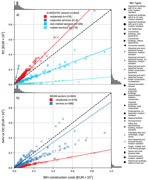
Comparing asset-to-asset, Fig. 8 presents the two LoD1-geometry distributed asset value model workflows against the BKI (2021) construction-cost benchmark dataset (also LoD1-geometry distributed). Because this benchmark dataset is drawn from a single, predominantly residential region, it is likely not representative of areas where industrial and service buildings are more prevalent.

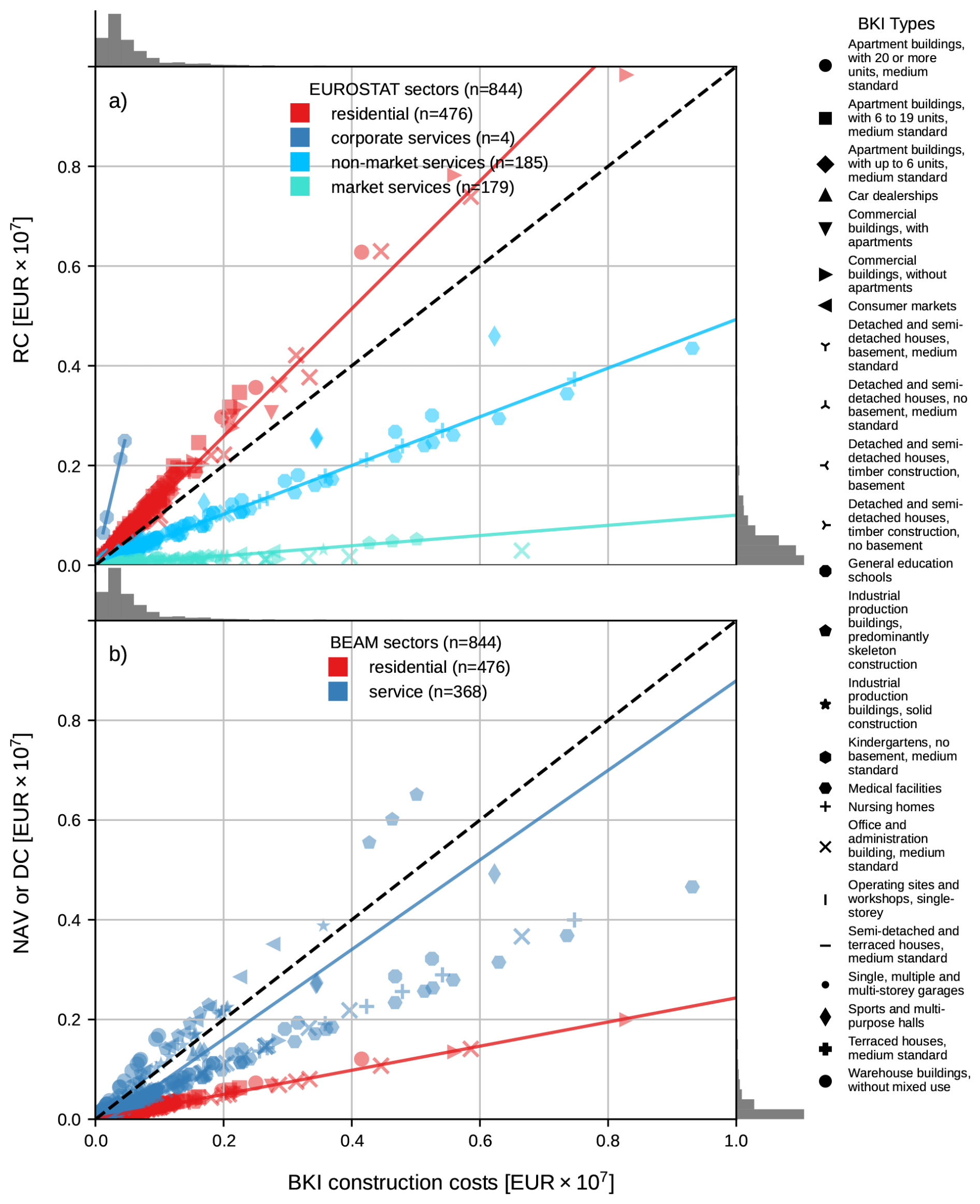
Figure 8 Asset values for (a) LoD1 + Eurostat (RC) and (b) LoD1 + BEAM (residential is DC while non-residential is NAV) workflows against the benchmark dataset. Markers represent the BKI (2021) type; colours represent the assigned sector. Solid lines provide the linear trend of the respective sector while the dashed line shows a 1:1 reference. Distributions of respective asset values are shown as histograms adjacent to the axes. RC: Replacement Cost, NAV: Net Asset Value, DC: Depreciated Costs.

Figure 8 shows a near-linear relationship between modelled and benchmark dataset asset values for all sectors, which is intuitive if we consider that both the workflows and the benchmark dataset are geometry-based; i.e., they differ mainly in the unit cost multipliers applied to the building area or volume (see Tables 4 and S9 for unit costs).

Setting aside the sectors with implausible disaggregated unit rates (e.g., market services and corporate services), most non-residential assets in the LoD1 + Eurostat workflow underestimate the benchmark dataset. This can also be seen by comparing the non-market services unit cost (EUR 251 m⁻³) to the BKI service unit costs (Table S9), nearly all of which are higher. This non-residential underestimation likely arises from LoD1 + Eurostat's reliance on stock-average values (Paprotny et al., 2020a), in contrast to the new-build construction cost averages reported by BKI.

Surprisingly, we find that the Eurostat residential asset values do not follow the same pattern and are generally higher than the benchmark dataset. This overestimate is likely influenced by the method we used to calculate the usable floor area, which multiplies the LoD1 footprint area by a height-derived storey count and a 0.7 usable-area coefficient after Paprotny et al. (2020b). Figure S5 shows the lack of precision of the storey counts estimated in this way, which generally exceed the observed benchmark dataset counts, in some cases by three storeys, inflating usable floor area and therefore residential RC at the object level. Further, sensitivity to the area multiplier is substantial. For example, using LoD1 footprint area directly gives a residential RC roughly EUR 14.5 billion (56 %) lower than the usable floor area estimates used here.

Conversely, all residential BEAM assets underestimate their BKI counterparts, with a unit cost of EUR 118 m⁻³, lower than any reported by BKI. While this is unsurprising considering BEAM includes a depreciation factor, the modest residential over-assignment (62 false positives; Table S11) could also influence the discrepancy. In contrast, the LoD1 + BEAM service assets are less biased, with the EUR 295 m⁻³ falling within BKI's wide range (Table S9); however, this results in higher variance than the other sectors. Thus, these differences should be read primarily as conceptual alignment with stock-average or depreciated values rather than inherent model deficiency; with the available data, we cannot isolate the specific mechanisms driving each discrepancy.

Unlike the LoD1-based workflows and the benchmark dataset, EHRE is object- rather than geometry-distributed, assigning asset values using probabilistic construction types from ESRM20's regional totals. In other words, EHRE preserves regional average replacement costs (from ESRM20) whereas the LoD1-based workflows considered here preserve asset-level unit costs. Further, EHRE's OSM geometry basis provides a simpler, more consolidated footprint-based representation of buildings, whereas LoD1 – designed for 3D buildings – represents complex buildings with multiple features; consequently, building-by-building value comparison is subjective and challenging (unlike categorical comparison). Even the relatively similar aggregate inventories in Table 4 (LoD1: 61 756 buildings; EHRE with remainder: 65 056.9, 5.3 % higher) mask important differences in object definition and sector composition, so total count agreement should not be interpreted as asset-level comparability across LoD1 and EHRE. Our early attempts to address this evaluation challenge failed to find a satisfactory definition of a building object between the two datasets (esp. for large complex structures), but in general we found EHRE strongly under-estimates residential replacement costs, while commercial and industrial comparisons are more difficult to interpret because of small sample sizes and object-matching ambiguity. The open-source nature of EHRE and the ESRM20 exposure model it builds upon mean, however, that the performance of the EHRE model in this regard could be improved, firstly, by changing the average replacement cost per area and, secondly, by using the area of the OSM building footprints to calculate the replacement costs, instead of retaining ESRM20's average per-asset-type replacement costs (which are based on average building areas). Future work should explore frameworks for comparing complex and disparate asset value models like these; ideally in a way that balances complexity with interpretability.

3.4 Weighted Scoring Model

To provide a more robust basis for model selection we use a semi-quantitative Weighted Scoring Model (WSM) to communicate the relative strengths and weaknesses of the three exposure model workflows presented above. Derived from the multiple-criteria decision-making mathematical framework, this technique is widely used to prioritise options by assigning weights to various criteria, which are then scored and ranked (Zionts, 1981). For this, we developed the criteria and weights shown in Table S13 to inform decisions on model selection based on previous experience. As presented in Table 5, each workflow is scored on a scale of 0–10 for each criterion before scores are multiplied by their respective weights, then summed. The benchmark dataset classification score was calculated from Table S12, while the criterion weights and remaining workflow scores were assigned through iterative discussion among the authors until consensus was reached on a final set of values.

Table 5 Scores and weights for the asset value model workflows. See Table S13 for a description of each criterion.

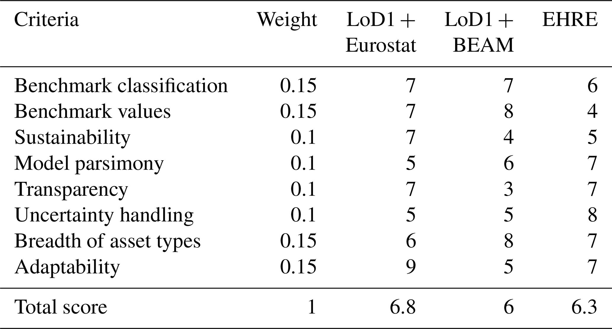
In the WSM, LoD1 + Eurostat slightly outperforms the other workflows owing mainly to its benchmark dataset performance, sustainability, and adaptability.

Eurostat data are updated annually, offering a clear advantage, whereas the update cycles of BEAM are unclear and EHRE currently has no planned updates. Like BEAM, Eurostat data tables are web-hosted with open access; however, the LoD1 data requires a licence (commonly provided for free to public bodies and research institutes under specific agreements), while commercial users typically obtain fee-based licences.

Of the asset value model workflows considered, LoD1 + Eurostat is more onerous than LoD1 + BEAM, requiring the downloading and disaggregation of regional and categorical estimates (see Eq. 1). EHRE, on the other hand, is already disaggregated to per-asset stochastic classes; therefore pre-processing is only required if the user desires deterministic values (like our study).

Considering the transparency of the underlying data, BEAM is substantially more opaque than the other workflows, with no source code or parameter values provided and documentation only a short paragraph, in some cases without references. In contrast, we find LoD1 + Eurostat and EHRE similarly transparent, both relying on large-scale opaque source data (e.g., OSM, LoD1) but with subsequent calculations performed transparently. For example, the EHRE source code is published (Nievas et al., 2023) while the simpler LoD1 + Eurostat workflow is described by Fig. 3 and Eq. (1).

EHRE is the only workflow to explicitly consider uncertainty, both through the incorporation of probabilistic building types and the use of remainder layers and the other building sector.

Finally, while our study focuses on building structural asset values, numerous other asset types are often incorporated into exposure models (e.g., population, building contents). In this regard, LoD1 + Eurostat provides the narrowest set of asset types as it is the least pre-processed for exposure modelling.

However, this minimal processing affords the greatest flexibility for LoD1 + Eurostat, which provides data for any year across the Eurozone, allowing advanced modellers to tune the workflow for their context.

3.5 Limitations and recommendations

With this study, we provide the first per-asset evaluation of asset value model workflows for exposure modelling.

Although extending these workflows to other regions in Germany would be straightforward, the need for a labour-intensive hand-labelled benchmark dataset restricted our evaluation to a single region, meaning the findings are only transferable to regions with construction practices, economic conditions, and exposure distributions comparable to Ahrweiler. Future studies with more resources should consider extending the breadth and coverage of our benchmark dataset.

Similarly, we chose to focus on asset values and sector classification as the simplest means for comparing diverse workflows; however, exposure models typically include additional variables like building size, construction type, construction materials, etc. Including these, and non-building assets, in the benchmark dataset and evaluation would provide a more complete comparison. However, as the significance of each of these variables will depend on the particulars of the hazard in question and its associated vulnerability model, the usefulness of such a general study (rather than one specific to a particular case) should be carefully considered. Further, these additional variables are rarely ingested by loss models, and therefore their inclusion in our evaluation would be of limited use to most readers.

The dependence of our benchmark dataset on the underlying BKI (2021) data, which only provides average new construction costs in Germany, makes the comparison less useful for certain disaster modelling applications like estimating insurance claims or disaster reconstruction for a heterogeneous set of buildings. More useful would be observed replacement costs from disaster-affected buildings; however, this information is notoriously difficult to collect and plagued with uncertainty when self-reported (Rözer et al., 2019).

For the LoD1 + Eurostat residential estimate in particular, the reliance on inferred rather than observed usable floor area introduces uncertainty and complexity: future work should improve this conversion.

Similarly, because we opted to provide a broad evaluation, we include asset value model workflows with different cost bases (RC, DC, NAV) and years (2018, 2020, and 2022), making our findings less conclusive.

Aligning cost bases or developing standardised conversion approaches could improve the comparability of the evaluation, but at the expense of attribution and interpretability.

While our work only considers classical disaggregation workflows built on standard accounting and cadastral datasets, the challenges reported here suggest opportunities for employing machine-learning and remote-sensing-based methods, especially for asset classification.

For example, Gouveia et al. (2024) and Silva et al. (2024) trained algorithms on labelled images of buildings with promising results.

Lastly, during data collection and publication we struggled to obtain and release asset-level data, a challenge commonly faced by European exposure modellers. This type of building-level economic data is generally considered to be privacy-protected under the EU's General Data Protection Regulation (European Union, 2016). While many benefits arise from such protections, policymakers should consider the burden this places on asset-level disaster modelling (McLennan et al., 2020).

4 Conclusions

This study developed and benchmarked object-level asset value model workflows for a region in Germany, examining various disaggregation approaches from cadastre-derived (LoD1), crowd-sourced (OSM), national accounts (Eurostat), and fit-for-purpose datasets (EHRE and BEAM). We adapted and extended four exposure model workflows and evaluated these with our hand-labelled benchmark dataset.

From this, we found that the cadastre-derived LoD1-based workflows performed best overall against the benchmark dataset at labelling a building's sector (F1 = 0.71), but lacked the resolution necessary to identify industrial uses. This contrast between strong residential performance and near-complete failure for industrial assets indicates a limitation of cadastral function categories rather than a modelling error. It also cautions against the uncritical use of authoritative building function data for economic sector classification.

Aggregate, region-wide values diverged between the candidate workflows (up to an order-of-magnitude at the sector level), suggesting an under-appreciated level of uncertainty – comparable to uncertainties reported in other aspects of risk modelling, like vulnerability – and emphasising the need for local validation.

Similarly, we found implausible unit rates when disaggregating regional sector totals onto LoD1 functions that poorly represent our local sector mix (e.g., unit costs hundreds of times beyond comparable published values), signalling the importance of aligning regional data with building-level data.

Setting these implausible unit rates aside, we found BEAM and most non-residential LoD1 + Eurostat values underestimate the new construction costs reported by our benchmark dataset, while LoD1 + Eurostat residential values are generally higher. This likely reflects, respectively, BEAM's inclusion of depreciation, Eurostat's reliance on stock-average replacement costs rather than new-build price lists, and the sensitivity of residential estimates to usable-floor-area assumptions.

Extending this evaluation using a scoring model to examine less-quantitative factors important for exposure modelling like sustainability, transparency, and adaptability, we find all candidate workflows (except the land-use-based workflow) obtain similar total scores. However, the LoD1 + Eurostat workflow performs slightly better, mainly due to its ease of adaptation across regions and time periods, and the relative simplicity of maintaining and updating it.

These findings suggest that, other than the land-use-based workflow, any of the three asset value model workflows can provide a defensible asset-level exposure model in Germany, albeit with different cost bases. Modellers should select the workflow that aligns with their sustainability, adaptability, sophistication, and cost-basis needs and perform local validation. In summary, we find transparent, maintainable workflows, not coarse land-use proxies, yield the most reliable object-level exposure when grounded in local validation.