A fluvial flood risk model for quantifying the benefit of mitigation measures under uncertainty

We present a dynamic probabilistic flood risk model that addresses key challenges in the implementation of integrated flood risk management. These include the need for holistic, large-scale risk assessments that adopt a system-based perspective, and a decision-making framework based on benefit-cost analysis. The proposed model allows for the explicit representation and dynamic coupling of the flood process components, including downstream flood wave propagation and possible dike failures, in a computationally efficient and data-sparse manner. This enables the consideration of aleatory and epistemic uncertainties in a 2-level Monte Carlo framework. By separating these uncertainties, the model supports robust risk assessments and facilitates an uncertainty-aware evaluation of the benefit of mitigation measures. The model is applied to the Bavarian Danube, demonstrating its ability to estimate the flood risk-reduction potential of mitigation measures.

1 Introduction

Over the past few decades, the approach to flood management has transitioned from a mainly technical focus on flood protection to a more comprehensive flood risk management strategy (Vitale, 2023; Thomas and Knüppe, 2016). This shift was catalyzed by significant flood events, such as the catastrophic 2002 flood in Central Europe, which traditional flood protection measures failed to prevent. With estimated direct damages of EUR 22.6 billion (reference year 2005; Petrow et al., 2006), the 2002 flood stands as the most expensive natural hazard event recorded in Germany. In response, numerous administrative and legislative initiatives were launched at both the EU and national levels to enhance preparedness for future flooding (Thieken et al., 2016). However, subsequent flood events in 2013, 2021, and 2024 have highlighted the need for further advancements in the implementation of integrated flood risk management, which can be summarized by three necessary key developments (Merz et al., 2010a):

1. Comprehensive risk assessment: While traditional engineering approaches relied on predefined design floods and corresponding protection levels (Messner et al., 2007), flood risk management encompasses the entire spectrum of potential flood events and their uncertain consequences. It acknowledges the possibility of flood protection failures, even below established design standards, and recognizes that absolute safety against flooding is unattainable. Deterministic models, which assume fixed relationships between return periods, water levels, and flood damage, are increasingly insufficient. Recent studies have highlighted the downstream impacts of dike failures (Apel et al., 2009b; Curran et al., 2020). Consequently, flood risk assessments must explicitly model the flood process chain and dynamically couple its components. Different aleatory uncertainties, arising from natural variability, exist in these components, which are traditionally represented in flood risk models (Hall and Solomatine, 2008). Alongside these aleatory uncertainties, epistemic uncertainties, i.e., uncertainties resulting from incomplete knowledge and model imperfections inherent in every flood risk model, must be addressed (Apel et al., 2008). There is a scientific consensus advocating for probabilistic approaches to enhance robust flood risk assessment and estimate the impact of uncertainties (Domeneghetti et al., 2013; Apel et al., 2004; Hall and Solomatine, 2008; Merz and Thieken, 2009).

2. Shift in decision-making criteria: Decision-making processes must move from regulation-based frameworks to performance-based approaches, wherein the potential for flood risk reduction is weighted against the costs of mitigation measures (Messner et al., 2007). This criterion promotes a more transparent and cost-effective allocation of limited resources (Gamper et al., 2006). To evaluate the benefits of mitigation measures, flood risk must be estimated both with and without their implementation. Therefore, a model capable of simulating the impacts of mitigation measures – at the site of implementation as well as downstream – is essential. Both aleatory and epistemic uncertainties should be integrated and communicated within benefit-cost analyses (Hall and Solomatine, 2008). Decision-oriented sensitivity studies (Straub et al., 2025) can further enhance the decision-making process, ensuring robustness and transparency.

3. Integrated, cross-border approaches: It is increasingly recognized that isolated, local flood protection strategies must be replaced by integrated approaches that frame flood risk mitigation as a comprehensive task spanning large spatial scales and involving multiple riparian communities (Thieken et al., 2016). Local flood mitigation efforts can have trans-local consequences (Metin et al., 2018). Dikes may temporally and spatially shift flood hazard, potentially exacerbating flood risk downstream. Other flood protection measures, such as detention basins, are designed in a way that their impact propagates far downstream (Förster et al., 2005). Ignoring these interdependencies can undermine the optimal allocation of resources and diminish risk reduction potential. Moreover, integrated flood risk management encompasses not only technical solutions but also a diversification of management strategies, including spatial planning, early warning systems, nature-based solutions, and flood-proofing (Merz et al., 2010a). Despite decades of research advocating for integrated flood risk management, decision-making and its practical implementation often remain fragmented across various professional sectors that focus on local flood protection planning.

These three developments require flood risk models that can represent interactions in flood processes, provide uncertainty-aware risk estimates, and operate at river or catchment scale. In the scientific literature, different models have been presented that meet one or more of these criteria. The first probabilistic national-scale flood risk assessment in England was developed by Hall et al. (2003). In this model, dike reliability is represented using fragility functions, which are coupled with a static inundation model to estimate expected annual flood risk across different regions. A basic uncertainty analysis is included to provide upper and lower bounds on the estimated risk. This methodology was further enhanced by Gouldby et al. (2008) at a regional scale, where the fragility functions were refined and hydraulic load scenarios probabilistically generated from extreme value distributions. However, both models lack dynamic coupling between components and, consequently, do not account for downstream discharge reductions following dike failures. Another model developed by Apel et al. (2004), applied to the Rhine River in North Rhine-Westphalia, Germany, incorporates hydrological load scenarios derived from a flood frequency curve, Muskingum-based flood routing, levee breach and outflow modeling as well as a static inundation and damage assessment. Dike failure due to overtopping is modeled using a 2D fragility function derived via Monte Carlo simulation of a limit state function under uncertain dike properties. However, breach assessment is limited to only two locations. Subsequent extensions of this model introduced uncertainty analysis (Apel et al., 2006, 2008) and allowed for quasi-continuous dike breach locations (Apel et al., 2009b). Similarly, the flood risk model developed by de Kok and Grossmann (2010) for the Elbe River in Germany integrates scaled synthetic flood events (based on predefined return periods), a dike breach module, a 1D hydraulic flood routing model, and a macro-scale economic damage assessment. Dike breaches are assumed to occur deterministically as a result of overtopping. While this approach allows for scenario-based risk assessment, it does not include a formal uncertainty analysis. More recently, the Germany-wide flood risk assessment by Sairam et al. (2021) employs a flood event catalog derived from 5000 years of hydro-meteorological simulation data, coupled with a 1D-2D hydrodynamic model to simulate flood propagation and inundation as a consequence of dike overtopping. Dike failure and its consequences are not included, but a comprehensive uncertainty analysis is conducted. The flood hazard model of Apel et al. (2009a) was further refined by Vorogushyn et al. (2010) and extended by the failure mechanisms piping and micro-instability. Moreover, the original flood routing approach was replaced with a 1D hydrodynamic simulation, and the inundation assessment upgraded to a 2D storage-cell-based hydrodynamic model. These enhancements necessitate runtime coupling of the probabilistic model with process-based simulations, increasing the degree of process representation. Domeneghetti et al. (2013) applied this advanced model to a 50 km reach of the Po river in Italy, demonstrating its capability for probabilistic flood hazard mapping under uncertainty.

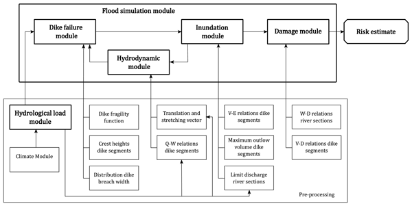
This overview of existing large-scale flood models highlights the necessary trade-off among modeling complexity, spatial extent, and comprehensiveness of the uncertainty analysis. In this work, we introduce a probabilistic flood-risk model that seeks an effective balance between these three objectives. The developed model achieves computational efficiency by replacing runtime coupling of computationally expensive hydraulic and hydrodynamic simulations with pre-processed surrogates and lookup tables, while still dynamically coupling flood-process components (Fig. 2). This allows the model to represent the key process interactions, without the prohibitive runtime associated with coupled simulation models. Crucially, the model explicitly captures downstream propagation of impacts following dike failures or activation of mitigation measures, such as controlled detention basins (Sect. 5), via an efficient flood-routing scheme. The resulting computational efficiency enables embedding the risk model within a two-level Monte Carlo framework. Aleatory and epistemic uncertainties are introduced and propagated separately, thereby enabling a more comprehensive uncertainty and sensitivity analysis than previously feasible at river scales.

The reduction in modeling fidelity compared with flood risk models coupled with high-resolution hydraulic simulations is, as we argue, acceptable in many decision-making contexts, particularly when uncertainty is explicitly quantified within a consistent framework. It is important to note that the primary contribution of this work is methodological: the objective is to develop and present a novel modeling framework, rather than to provide a definitive flood risk assessment for a specific river reach.

To demonstrate the applicability of the proposed framework in real-world decision contexts, it is applied to the Bavarian Danube in a case study, where the benefit of a flood mitigation measure and its associated uncertainty is estimated. The successful application in the case study proves that the model can (i) provide large-scale probabilistic risk assessments, (ii) support decision-making through uncertainty-aware quantification of risk reduction, and (iii) explicitly model interactions between mitigation measures and downstream effects, which provides the basis for joint optimization of mitigation portfolios at river scale.

The remainder of the paper is organized as follows. Section 2 introduces the exemplary study area, Sect. 3 outlines the components of the flood risk model, Sect. 4 describes the two-level Monte-Carlo framework and Sect. 5 presents results from the application of the model to an exemplary decision-making context. The paper concludes with a discussion and remarks in Sect. 6.

2 Study area

The study area utilized in this work to develop, test and demonstrate the application of the flood risk model is the Bavarian part of the Danube River, Germany, shown in Fig. 1. The Danube originates in Baden-Württemberg in western Germany, flowing for approximately 380 km through Bavaria before crossing the border into Austria, east of Passau. The river's hydrology is heavily influenced by its tributaries, many of which originate in the Alps, including the Iller, Lech, Isar, and Inn rivers. In addition, the northern catchment area is fed by key tributaries such as the Wörnitz, Altmühl, Naab, and Regen rivers, which arise in the Central German Uplands. Notably, flood dynamics in the northern and southern catchment areas of the Danube differ in terms of underlying formation mechanisms and seasonal patterns, which, in turn, affect flood wave characteristics. This plays an important role in shaping the overall flood hazard associated with the Bavarian Danube. Approximately 54 % of the catchment area is used for agriculture, 34 % is covered by forests, and 13 % is urbanized. Significant industrial centers, including Donauwörth, Ingolstadt, and Regensburg, are located along the river. The cities Regensburg and Ingolstadt are the third and fourth most populous cities in Bavaria.

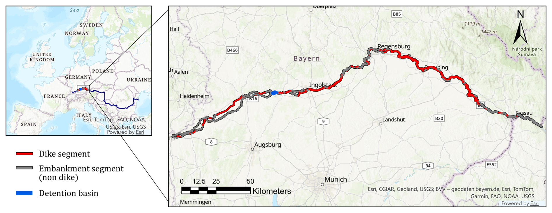
Figure 1 Overview of the study area.

In the case study (Sect. 5), the risk reduction potential of a controlled detention basin located near Riedensheim (blue area in Fig. 1) is evaluated using the developed model. Controlled detention basins are operated by diverting water from the river into the polder area during extreme events, temporarily storing flood volumes and thereby attenuating the flood wave and reducing downstream peak discharges. After the flood peak has passed, the stored water is gradually released back into the river system. The evaluated basin can store a volume of around 8×10⁶ m³ with a maximum intake capacity of 170 m³ s⁻¹. Its operating mode is built into the flood simulation model and follows predefined rules, assuming perfect forecasts. It is activated if a 100-year flood is exceeded at or directly downstream of its location in order to relieve the basic flood protection downstream. For flood events below a 100-year flood, the detention basin is not activated, as the existing basic flood protection is considered sufficient to withstand such events. The exemplary analysis focuses on quantifying the expected reduction in flood risk attributable to the operation of the detention basin, including its associated uncertainty. This benefit can subsequently be weighed against the construction and operation costs of the measure to support economic decision-making.

3 Flood risk model

The developed flood risk model comprises five primary modules that collectively represent the flood process: the hydrological load module, the dike failure module, the hydrodynamic module, the inundation module, and the damage module. Among these, the dike failure, hydrodynamic, and inundation modules are dynamically coupled to enable updates between them during simulation runs. The flood risk model is summarized in Fig. 2 and further explained in the following sections. It is integrated within a 2-level Monte Carlo framework, which distinguishes between aleatory and epistemic uncertainty (see Sect. 4). To optimize computational efficiency, all modules utilize pre-computed runs from various modeling tools, as indicated by the pre-processing box in Fig. 2.

Figure 2 Schematic overview of the flood risk model. Q: discharge, W: water level, V: volume, E: elevation, D: damage.

To apply the flood risk model to a specific case study, several preparatory steps must be undertaken. Although these steps are exemplified for the Bavarian Danube study area, they can be easily adapted to other catchments. First, the river and its surrounding foreland are contained on both sides by a longitudinal embankment line. In areas where river dikes exist, this embankment line coincides with their alignment; in other locations, it follows the outline of the 100-year flood-plain obtained from official flood hazard maps. Second, the river and its longitudinal embankment line are laterally discretized into sections ranging from 300 to 600 m in length, following the recommendations of CUR/TAW (1990). This choice ensures that the response of dikes segments of this length to hydraulic loading is approximately independent of its adjoining segments (Vorogushyn et al., 2010). Additionally, the river reach is longitudinally divided into two parts to model river bifurcations. As a result of this discretization process, a total of 2×892 river segments are defined along the Bavarian Danube. The adjacent longitudinal structures are termed embankment segments, which are further categorized as either dike or non-dike segments. Similar to Apel et al. (2009b), dike segments with overlapping hypothetical inundation areas are grouped together into impact zones. Figure 3 illustrates the spatial structure of the model. The segmentation and zoning enables efficient modeling of the flood process but introduce model inaccuracies, such as the overestimation of water heights when flooding exceeds the extent of the 100-year event, which is quantified in the uncertainty analysis.

Figure 3 Schematic spatial discretization structure of the river.

3.1 Hydrological load module

Flood hazard can be characterized by a range of representative flood scenarios, each associated with a specific occurrence probability. The derivation of these flood scenarios can be accomplished through various approaches. While early flood risk assessments predominantly relied on historical or design hydrographs, these approaches have mostly been replaced by the synthetic generation of flood waves based on (multi-variate) distributions (Curran et al., 2020), climate-based precipitation simulations (Sairam et al., 2021) or synthetic weather generators (Merz et al., 2024; Guan et al., 2025). Methods that depend on historical observations often face challenges in extrapolation, particularly when predicting flood events and their probabilities beyond the range of observed data. Various extreme value statistics and clustering methods have been employed in the literature to derive synthetic hydrographs based on flood frequency analyses (Vorogushyn et al., 2010). By contrast, climate-based precipitation simulations and synthetic weather generators are theoretically independent of specific historical flood events and thus offer the greatest potential for representing flood hazard beyond the range of observed records (Ludwig et al., 2019). Simulated flood events often undergo post-processing – such as rescaling or adjustment of occurrence rates – for bias correction based on historical observations; in practice, they are not entirely independent of past events.

In the current study, a set of flood events is derived from the ClimEx project, which conducted quasi-random climate-based simulations of hydrometeorological events in Bavaria (Ludwig et al., 2019). A total of 50 transient simulations over the time horizon of 1980 to 2099 were carried out, employing the IPCC emission scenario RCP8.5 (IPCC, 2013). From these simulations, 3500 years of precipitation data covering the period from 1980 to 2050 are extracted. Hence, the selected precipitation events reflect the climatic conditions of the recent past, present, and the near future relative to the reference year 2020 of the study. The decision to exclude simulations beyond this period is based on the significant uncertainties associated with future climatic conditions and their potential impact on precipitation patterns. Uncertainty in flood frequency resulting from climate change impact is investigated in the scenario analysis presented in Sect. 5.

Following intermediate simulations of runoff generation using WaSim (Schulla and Jasper, 2007) and flood routing within the catchment via Larsim (Bremicker, 2000), 72 flood events are identified that exceed a 100-year event on at least one of the gauging stations along the Bavarian Danube. The detention basin evaluated in this study (introduced in Sect. 2) is designed to be activated only when discharges exceed the threshold of a 100-year event. The measure does not change the risk for events with lower discharges; therefore, these events do not need to be included in the analysis. If mitigation measures operating at lower discharges are to be assessed, the flood event catalog must be extended accordingly. The identified flood events can be interpreted as Monte Carlo samples of flood occurrences for which the evaluated measure provides a benefit, representing the aleatory uncertainty (randomness) associated with the flood event. The occurrence rate of these flood events is estimated as $\mathit{\lambda }=\mathrm{72}/\mathrm{3500}$ yr⁻¹. The 72 flood events are subsequently routed through the Danube River channel using the 1D non-stationary hydraulic modeling tool SOBEK (Deltares, 2018). Each river segment is linked to a hydraulic SOBEK node, ensuring that the flood events are spatially discretized according to the model's resolution. A temporal resolution of 1 h is used in the flood risk model. In case of unbifurcated river channels, the two segments of a river section are linked to the same SOBEK node; in the bifuricated case, different nodes are assigned to the two opposite segments of a river section. For illustration, 19 flood events are depicted in Fig. 4 at four exemplary segments along the Bavarian Danube.

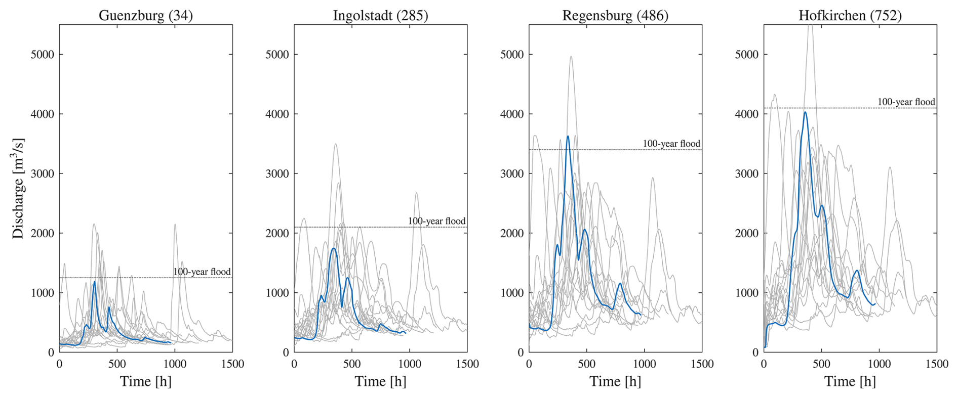
Figure 4 Hydrograph of 19 exemplary flood events at four locations along the Bavarian Danube. Segment number of location in brackets. One randomly chosen flood event is shown in blue.

In addition to discharges Q along the river network, the hydraulic simulations provide corresponding water levels W. For each river segment, an empirical stage–discharge relationship is derived by binning simulated Q–W pairs from all flood events based on discharge values. Within each bin, mean discharge and water level values are calculated to construct a discretized stage-discharge curve. In the flood simulation model, water levels are then estimated via piecewise linear interpolation between these values. While computationally efficient, this method assumes a single-valued Q–W relationship and therefore does not capture hysteresis effects, which is quantified in the uncertainty analysis.

3.2 Dike failure module

Dikes are most likely to fail when water levels significantly exceed design specifications. In this study, failure refers to the physical breach or collapse of the dike, while overtopping denotes the overflow of water across the dike crest without implying structural damage. Failure resulting from overtopping is implicitly accounted for through the fragility function, as outlined below. Dike failures can result in catastrophic damage, especially when affecting densely populated areas, a phenomenon often referred to as the ”levee effect”. Studies have extensively investigated the relationship between dike breaches and flood damage, underscoring the importance of understanding dike reliability (Vorogushyn, 2008; Curran et al., 2019; Gouldby et al., 2008). The reliability of dike systems can be assessed through three primary approaches: empirical analyses, expert judgment, and model-based probabilistic analyses (Schultz et al., 2010). First efforts to systematically quantify the probability of dike failure using fragility functions were made by the U.S. Army Corps of Engineers in the early 1990s (USACE, 1991). Since then, considerable research has been conducted, and model-based probabilistic approaches have gained significant traction in the field. Dike failure modes can be categorized into three primary types: hydraulic, geohydraulic, and global static failure (Vorogushyn, 2008). Hydraulic failure occurs when overtopping water erodes the dike material from the landward side. If wave-induced overtopping is neglected – an assumption adopted by Vorogushyn (2008), Apel et al. (2004), and Domeneghetti et al. (2013) – the probability of hydraulic failure is zero for water levels below the dike crest height. Geohydraulic failure arises from an uplift of the dike core, typically resulting from piping processes occurring in the dike foundation. In contrast, global static failure is induced by microinstability within the dike core due to internal seepage processes. A comprehensive study of the analytical description of dike failure modes was conducted by Vorogushyn (2008).

Vorogushyn (2008) describes the physical processes leading to failure through the use of limit state functions, which typically compare the stress S acting on a structure with its resistance R: $g(R,S)=R-S$. Failure occurs if $g(R,S)\le \mathrm{0}$, i.e., when S exceeds R. Both R and S are treated as uncertain and are characterized by a range of random variables corresponding to different dike properties. For the three distinct failure modes, different (conditional) sub-mechanisms are incorporated into the limit state function. In this work, the limit state functions for the (sub-)mechanisms contributing to g(R,S) are derived from the work of Vorogushyn (2008) and evaluated using a Monte Carlo simulation to generate fragility functions. For all random variables entering g(R,S) for which no site-specific data was available, probability distributions are based on Vorogushyn (2008). The resulting conditional failure probabilities are in function of various load variables, such as water level relative to crest height, overtopping duration, and impoundment duration. To reduce computational complexity and streamline the model, these variables are not directly evaluated in the flood simulation model. Instead, the fragility functions are evaluated in a pre-processing step at each dike segment independently, utilizing the flood events outlined in the hydrological load module in Sect. 3.1. By calculating the expected value of the failure probability conditional on the maximum water level relative to the crest height h_k of each dike segment, a fragility function is obtained that is conditional solely on the relative water level. This function incorporates all three failure mechanisms and implicitly contains information regarding the characteristics of the underlying flood scenarios. Hence the fragility function is specific for the considered study area and flood events. It is presented in Fig. 5 and applied to all dike segments. Uncertainty bounds are derived and used to define the lower and upper limits of the beta distribution employed in the uncertainty analysis (Sect. 5). If more detailed information regarding the dike characteristic is available, this generic fragility function can be updated.

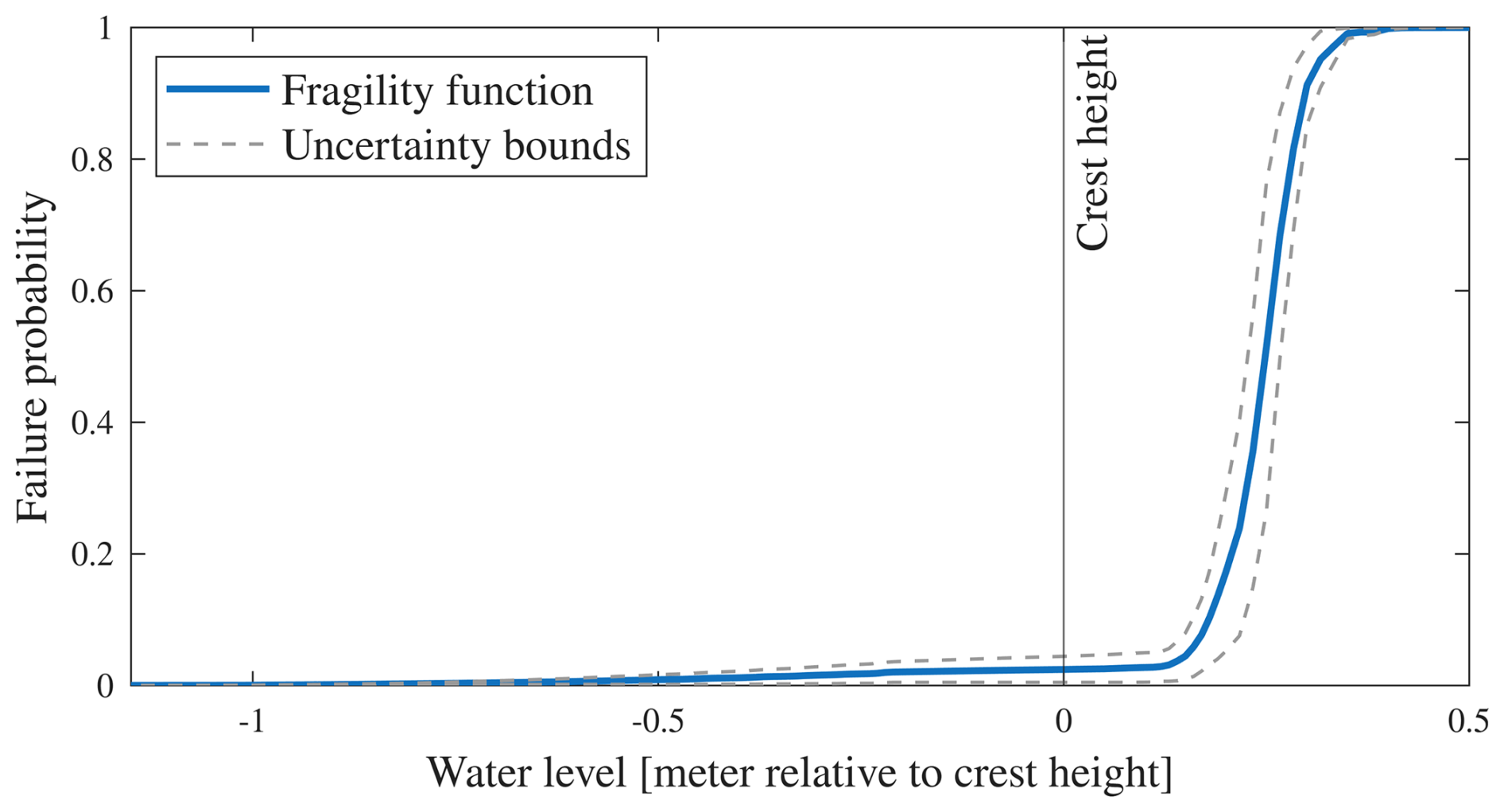
Figure 5 Developed fragility function P_F(w) and its uncertainty bounds for single dike segments. This function is specific to the case study.

In the flood simulation model, the fragility function is applied to every dike segment. In each Monte Carlo sample run, a breach resistance value r – defined as the maximum water level the segment can withstand before failure – is sampled by inverse transform sampling using the fragility function. Specifically, a uniform random variable $U\sim \mathcal{U}(\mathrm{0},\mathrm{1})$ is drawn and mapped to a water level w^∗ via the inverse fragility function, $r=w^{\ast }=P_{\mathrm{F}}^{-\mathrm{1}}\left(U\right)$. The resistances of dike segments are considered independent of one another, justified by the rationale for the choice of segment length outlined in Sect. 3. Dike failure is defined to occur when the water level, at any time during the flood event, exceeds the breach resistance r. In case of breaching, the breach width b is quasi-randomly sampled from a lognormal distribution with parameters μ_b=58.5 m and σ_b=61.3 m, following Vorogushyn (2008). If the sampled breach width falls outside the range [3 m,b_s], with b_s equal to the segment width, it is truncated to conform to these limits. Thus, both breach resistance and breach width – and therefore the aleatory uncertainties inherent in the breaching process – are accounted for by the first-level Monte Carlo simulation. The breach development rate is assumed to be 1 h, consistent with the methodology employed by Apel et al. (2004, 2006) and Vorogushyn (2008). The breach is assumed to erode the entire dike down to the toe level of the dike, h_t.

3.3 Inundation module

The hourly outflow discharge through the dike breach (or overflow over the crest in the absence of failure) into the hinterland at time step t is calculated using a modified broad-crested weir equation:

$$\begin{array}{}\text{(1)}& Q_{\mathrm{out}}\left(t\right)=\mathrm{2}/\mathrm{3}\cdot {\mathit{\mu }}_{\mathrm{0}}\cdot {\mathit{\mu }}^{\ast }\cdot \sqrt{\mathrm{2}g}\cdot b\cdot h^{\mathrm{3}/\mathrm{2}}\left(t\right)\end{array}$$

where g [m s⁻²] is the gravitational force, h [m] the overfall height, μ₀=0.577 [–] the flow factor and ${\mathit{\mu }}^{\ast }=\mathrm{0.7}$ [–] a discharge reduction factor to account for the influence of the dike breach, motivated by the studies of Kamrath et al. (2006). The overfall height is

$$\begin{array}{}\text{(2)}& h\left(t\right)=\left\{\begin{array}{ll}{h}_{\mathrm{t}}+w\left(t\right)& \mathrm{for}\mathrm{breaching}\\ w\left(t\right)-h_{\mathrm{c}}& \mathrm{for}\mathrm{overtopping}\end{array}\right.\end{array}$$

with h_t and h_c the height of the dike toe and dike crest respectively, and w(t) the water level in the river segment. Discharge over the dike crest or through the dike breach is constrained. For each river segment, a limit discharge remaining in the river channel Q_l at both dike crest height and dike toe height is estimated in a pre-processing step based on the Q–W relationship obtained from the hydraulic simulation discussed in Sect. 3.1. With $Q_{\mathrm{out}}\left(t\right)=min\mathit{\left\{}{Q}_{\mathrm{out}}\right(t),Q_{\mathrm{river}}(t)-Q_{\mathrm{l}}\mathit{\}}$, it is ensured that the outflow does not exceed physically plausible limits, neglecting wave influence. Additionally, w(t) in the river segment is compared to the inundation elevation in the hinterland E_in(t) at the respective time step. Consequently, the model automatically switches between free and drowned overfall, depending on the water levels in the river and the hinterland. The outflow volume V(t) is approximated as the sum of the outflow discharges $V\left(t\right)={\sum }_{t^{\prime }=\mathrm{1}}^{t-\mathrm{1}}{Q}_{\mathrm{out}}\left(t^{\prime }\right)\cdot \mathrm{3600}$ s. Backwater discharges are not modeled directly; rather, the outflow volume is constrained by a segment-specific maximum volume V_max determined by the topography and the surrounding dike heights, which is further outlined below.

Inundation modeling aims at estimating the extent of flooding given the topography and the boundary conditions of the breach and can be conducted with varying degrees of detail. The choice depends on the available computational and data resources, the objectives and scale of the study area, as well as the level of detail of other components of the flood risk model. In their national-scale flood risk assessment, Hall et al. (2003) estimated flood extent using a simple approximation method, spreading the calculated flood volume while assuming an average flood depth and a semi-circular or trapezoidal outline shape. de Kok and Grossmann (2010) utilized pre-computed volume-storage functions based on a 100 × 100 m grid to determine inundation depths. For their study at the Rhine River in Germany, Apel et al. (2004, 2006) derived so-called damage functions prior to the Monte Carlo simulation, assuming a horizontal filling of the hinterland in 0.5 m increments. This approach involved intersecting a horizontal plane with the digital elevation model (DEM). Vorogushyn et al. (2010) simulated the inundation process at run time using a 2D raster-based diffusive wave model that solves the continuity and momentum equations. This study employed a DEM with a 50 × 50 m grid cell resolution and average, land-use-specific roughness values based on literature data. A similar approach was pursued in the Italian flood hazard study conducted by Domeneghetti et al. (2013) at the Po River.

In this work, the relationship between inundation elevation (E) and inundation volume (V) is derived statically for each dike segment using ArcGIS. The inundation volumes are derived from the intersections between a 5×5 m DEM and horizontal surfaces, representing the water level, at 0.1 m height increments. As a constraint, the algorithm assesses the connectivity of the resulting volumes with their corresponding dike segments, systematically removing any disconnected pools. Additionally, inundation areas are cut along tributaries. Five resulting inundation areas at breach segment 500 are depicted in Fig. 6. As a result, V–E tables and hypothetical inundation areas are created for each segment. Furthermore, segments with overlapping hypothetical inundation areas at reasonably high inundation elevations are grouped together into impact zones. To account for backwater effects, the maximum outflow volume for each dike segment V_max is derived based on a simple approximation. This is achieved by considering the terrain slope in the direction of river flow, the height of the downstream protective structures within the same impact zone, and the derived V–E relationship. Additionally, in case of several breaches in a single impact zone, it is assumed that water flows together and forms one inundation area. Hence, the sum of the individual outflow volumes is used for inundation elevation and damage estimation. Elevation and damage (D) estimations are conducted based on the V–E and V–D (see Sect. 3.5) relationships of all involved segments using the total volume. The lowest resulting elevation and the highest damage estimate are chosen as decisive. Exemplarily, the resulting relationship between volume V and elevation E for segment 500 downstream of Regensburg is depicted in Fig. 9. In analogy to the dike segments, inundation areas are derived for all river sections. As a constraint in the GIS-based derivation of inundation areas for river sections, the algorithm assesses the connectivity of the inundation surfaces with the river network.

Figure 6 Five exemplary inundation areas at breach segment 500 derived with static GIS approach. Inundation elevations are: 328, 329, 330, 331 and 331.8 m.

The simplified static approach offers the advantage that, in case of breaching or overtopping, no process-based simulation of the flood wave in the hinterland is needed. Instead, a computationally inexpensive interpolation is conducted for each time step of outflow discharge. This approach neglects flood hydraulics, e.g. the influence of terrain roughness, flow velocity, flow direction, and settlement structures on the propagation of the flood wave. The impact of these simplifications varies depending on the existing topography, as studied by Apel et al. (2009a). They concluded that for low dynamic river floods, the consequences of the inaccuracies resulting from static inundation modeling are small compared to those resulting from large-scale damage assessments. Given the comparably flat topography of the Bavarian Danube, floods are mainly low dynamic, which allows this simplified approach.

3.4 Hydrodynamic module

The influence of dike breaches on downstream flood hazard has been emphasized in several studies over the past two decades, e.g., Vorogushyn (2008), Curran et al. (2019), and Apel et al. (2009b). If not properly incorporated, the downstream flood hazard can be significantly overestimated. At the same time, flood protection measures, such as detention basins, are designed in a way that they take effect until far downstream (Förster et al., 2005). To model the influence of mitigation measures and possible protection failures on downstream flood hydrographs, different flood routing techniques can be incorporated into flood risk models in varying degrees of detail. de Kok and Grossmann (2010) employ an empirical quick routing model that multiplies the discharges by a dimensionless system function. This system function depends on the length of the river segment, as well as translation and diffusion coefficients. Apel et al. (2004) apply the Muskingum method for flood routing, estimating travel time and form parameters based on 1D hydraulic simulations. Vorogushyn et al. (2010) utilize an unsteady 1D hydrodynamic model based on the Saint-Venant equations and cross-sectional profiles for river flood routing.

In this work, a vector-based flood routing approach is developed, which is composed of a translational and attenuation vector. It efficiently updates temporally and spatially discretized discharges downstream of a failed dike or an activated detention basin. The derivation of translational and attenuation vector is calibrated using the hydraulic modeling outcomes of the 1D simulation, conducted in the scope of Sect. 3.1. The translational vector is defined as $\mathit{T}=(T_{\mathrm{1}},T_{\mathrm{2}},\mathrm{\dots },T_n)\in {\mathbb{N}}_{\mathrm{0}}^{\mathrm{1}\times n}$, where n=892 is the total number of river segments. Each entry T_i represents the mean travel time from the reference section 1 to segment i. T is derived from a set of N_sim=18 hydraulic simulations, where artificial discharge reductions are applied to the flood hydrographs at the most upstream segment, resulting in N_sim discharge matrices ${\mathbf{Q}}_{\mathrm{red}}^{\left(k\right)}\in {\mathbb{R}}^{N_t\times n}$. N_t is the number of time steps in a flood event k. For each flood event k, the discharge reduction ΔQ_i at segment i is defined as:

$$\begin{array}{}\text{(3)}& \mathrm{\Delta }{\mathit{Q}}_i^{\left(k\right)}={\mathit{Q}}_i^{\left(k\right)}-{\mathit{Q}}_{\mathrm{red},i}^{\left(k\right)},\end{array}$$

where ${\mathbf{Q}}_i^{\left(k\right)}\in {\mathbb{R}}^{N_t\times \mathrm{1}}$ is the original discharge matrix of event k at segment i. The time of maximum discharge reduction $t_i^{\left(k\right)}$ is extracted for each segment i:

$$\begin{array}{}\text{(4)}& t_i^{\left(k\right)}=\arg \underset{t}{max}\left\{\mathrm{\Delta }{Q}_i^{\left(k\right)}\left(t\right)\right\}\end{array}$$

A sliding-window median filter is applied to {t^(k)} for all simulations k, resulting in ${\stackrel{\mathrm{̃}}{\mathit{t}}}^{\left(k\right)}$. The final translational vector entries T_i∈T are computed as the mean of the median-smoothed values over all flood scenarios:

$$\begin{array}{}\text{(5)}& T_i={\displaystyle \frac{\mathrm{1}}{N_{\mathrm{sim}}}}\sum _{k=\mathrm{1}}^{N_{\mathrm{sim}}}{\stackrel{\mathrm{̃}}{t}}_i^{\left(k\right)}\end{array}$$

In the flood simulation module, the relative travel time between a breach segment b and a downstream segment i is then computed as

$$\begin{array}{}\text{(6)}& T_i^{\left(\mathrm{rel}\right)}=T_i-T_b\end{array}$$

Given a computed discharge reduction $\mathrm{\Delta }{\widehat{\mathit{Q}}}_b\in {\mathbb{R}}^{N_t\times \mathrm{1}}$ at the breach location b, the corresponding discharge reduction without retention and attenuation effects at each downstream segment i is computed by time-shifting ΔQ_b according to the relative travel time $T_i^{\left(\mathrm{rel}\right)}$, and applying the reduction across the relevant time steps t:

$$\begin{array}{}\text{(7)}& \begin{array}{rl}& Q_i^{\left(k\right)}\left(t\right)-\mathrm{\Delta }{\widehat{Q}}_b\left(t-T_i^{\left(\mathrm{rel}\right)}\right),\\ & \mathrm{for}\mathrm{all}i>b\mathrm{and}t\in \left[t_{\mathrm{B}}+T_i^{\left(\mathrm{rel}\right)},t_{\mathrm{B}}+T_i^{\left(\mathrm{rel}\right)}+N_{t_R}\right],\end{array}\end{array}$$

where t_B is the time instance of breaching and $N_{t_{\mathrm{B}}}$ the duration of breaching. To model retention and attenuation effects, an attenuation vector is defined as

$$\begin{array}{}\text{(8)}& \mathit{A}=(A_{\mathrm{1}},A_{\mathrm{2}},\mathrm{\dots },A_n)\in {\mathbb{N}}_{\mathrm{0}}^{\mathrm{1}\times n},\end{array}$$

where each entry A_i represents the temporal spread of the discharge reduction at segment i. For each segment i, the attenuation factor A_i defines a symmetric temporal window of size ${\mathit{\tau }}_i=\mathrm{2}\cdot A_i+\mathrm{1}$. The discharge reduction is then redistributed evenly across this window:

$$\begin{array}{}\text{(9)}& \begin{array}{rl}& {\widehat{Q}}_{\mathrm{red},i}\left(t\right)=Q_i^{\left(k\right)}\left(t\right)-\sum _{j=-A_i}^{A_i}{\displaystyle \frac{\mathrm{1}}{{\mathit{\tau }}_i}}\cdot \mathrm{\Delta }{\widehat{Q}}_b\left(t+j-T_i^{\left(\mathrm{rel}\right)}\right),\\ & \mathrm{for}\mathrm{all}i>b\mathrm{and}t\in \left[t_{\mathrm{B}}+T_i^{\left(\mathrm{rel}\right)},t_{\mathrm{B}}+T_i^{\left(\mathrm{rel}\right)}+N_{t_R}\right]\end{array}\end{array}$$

This operation preserves the total reduction volume while approximating the attenuation observed in the hydraulic simulations. The attenuation vector A is composed of a generic, segment-independent component A_g, and a segment-specific component A_s. The attenuation vector entry i given a discharge reduction at a location b is calculated as

$$\begin{array}{}\text{(10)}& A_i=A_{\mathrm{g},i}+A_{\mathrm{s},i}-A_{\mathrm{s},b}\end{array}$$

To derive the attenuation vector components, a set of N_sim=18 additional hydraulic simulations are performed, where artificial discharge reductions are applied at different locations in the river network. The optimal attenuation vector components $A_{\mathrm{g},i}^{\left(\mathrm{opt}\right)}$ and $A_{\mathrm{s},i}^{\left(\mathrm{opt}\right)}$ for each segment i are determined through a parameter search procedure that minimizes the global error between the 1D hydraulic model and the translated and attenuated discharge reductions applying the vector-based approach across all scenarios for a range of candidate values:

$$\begin{array}{}\text{(11)}& \begin{array}{rl}& \left[{\mathit{A}}_{\mathrm{g}}^{\left(\mathrm{opt}\right)},{\mathit{A}}_{\mathrm{s}}^{\left(\mathrm{opt}\right)}\right]=\\ & {\displaystyle \frac{\mathrm{1}}{N_{\mathrm{sim}}}}\sum _{k=\mathrm{1}}^{N_{\mathrm{sim}}}\arg \underset{{\mathit{A}}_{\mathrm{g}},{\mathit{A}}_{\mathrm{s}}}{min}\left\{\sum _{t=\mathrm{1}}^{N_t}\sum _{i=\mathrm{1}}^n{\left(Q_{\mathrm{red}}^{\left(k\right)}(t,i)-{\widehat{Q}}_{\mathrm{red}}^{\left(k\right)}(t,i)\right)}^{\mathrm{2}}\right\}\end{array}\end{array}$$

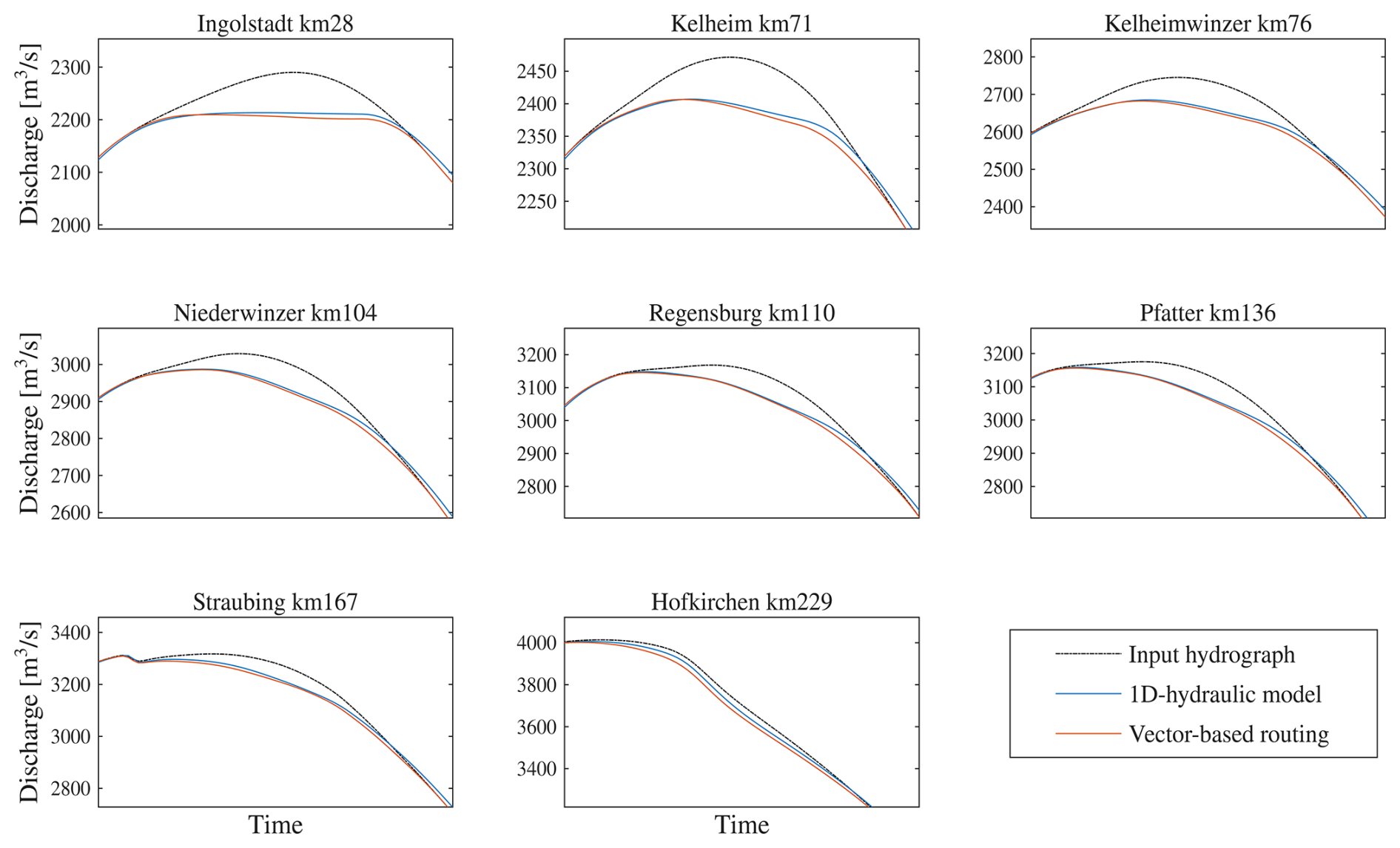
Figure 7 Comparison of 1D hydraulic SOBEK model results and vector based approach at 8 different locations. Kilometer values indicate distance to discharge reduction section. In black: Uncapped input hydrograph, in blue: propagated discharge reduction using 1D hydraulic model, in red: vector-based discharge reduction propagation.

The vector-based flood routing approach is tested using an independent set of 40 1D hydraulic simulations, in which the peak discharge is reduced by 8 × 10⁶ m³ at the location of the detention basin at segment 216, which is introduced in Sect. 5. The comparison of one resulting set of hydrographs at eight downstream segments is presented in Fig. 7.

Differences in peak discharge ΔQ relative to the vector-based peak discharge, temporal offset of peak discharge ΔT, absolute difference in peak water level ΔW, as well as the continuous Nash-Sutcliffe-Efficiency (NSE) criterion are evaluated at 15 downstream gauges for all 40 flood scenarios. The NSE is defined as

$$\begin{array}{}\text{(12)}& \mathrm{NSE}=\mathrm{1}-{\displaystyle \frac{{\sum }_{t=t_{\mathrm{start}\mathrm{fill}}}^{N_t}{\left(Q_{\mathrm{ref}}\left(t\right)-Q_{\mathrm{model}}\left(t\right)\right)}^{\mathrm{2}}}{{\sum }_{t_{\mathrm{start}\mathrm{fill}}}^{N_t}{\left(Q_{\mathrm{ref}}\left(t\right)-\stackrel{\mathrm{‾}}{Q_{\mathrm{ref}}\left(t\right)}\right)}^{\mathrm{2}}}}\end{array}$$

where model indicates the results of the vector-based propagation approach, ref those of the 1D hydraulic simulation that serve as the reference, t_start fill the first time instance at which the detention basin is filled (and the discharge downstream reduced) and N_t the total number of time steps. The resulting statistics of the quality criteria are shown in Fig. 8. They indicate that the differences between the hydraulic and vector-based routing results are low, especially compared to the discrepancy between the 1D and 2D hydraulic simulations.

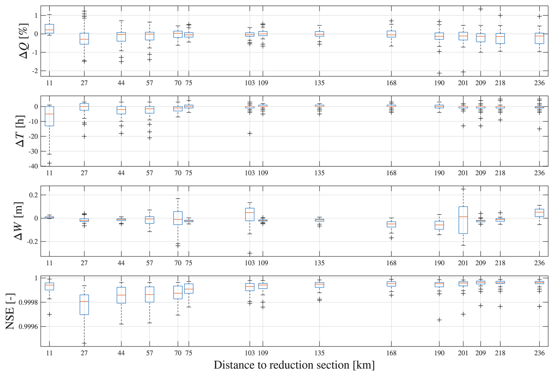
Figure 8 Quality criteria of vector-based flood routing approach, evaluated at 15 downstream segments. ΔQ refers to the difference in peak discharge between vector-based and 1D hydraulic simulation relative to the absolute peak discharge in the 1D simulation. ΔT is the temporal offset of the peak discharge [h], ΔW the absolute difference in peak water level [m], NSE the Nash-Sutcliffe-Efficiency of all discharge times series of the vector-based approach compared against the 1D hydraulic simulation.

At bifurcation points, where the river splits into multiple channels, the vector-based routing approach does not explicitly resolve travel time or retention differences between the diverging paths. However, discharge reductions must be accurately partitioned between different channels. To achieve this, a main reach and a threshold discharge Q_th are defined at each bifurcation segment. Secondary channels are activated only when the local discharge exceeds Q_th. The distribution of the discharge reduction is then determined using lookup tables Q_share, derived from the hydraulic simulations in Sect. 3.1. For each bifurcation segment, Q_share maps the effective discharge $Q_{\mathrm{eff}}\left(t\right)=Q\left(t\right)-Q_{\mathrm{th}}$ to a discharge split ratio across the available channels. This ensures that discharge reductions are apportioned consistently with observed flow behavior in the hydraulic model.

3.5 Damage module

Flood damages can be classified into direct and indirect damages and further subdivided into tangible and intangible damages (Merz et al., 2010a). The proposed flood risk model primarily addresses tangible damages. Considerable research has been conducted on direct tangible flood damage estimation, resulting in the introduction of various methodologies in recent years. Factors such as available data, understanding of damaging processes, study scale, and computational resources may limit the accuracy of direct tangible damage assessments. The general procedure for tangible flood damage assessment can be outlined in three steps (de Moel et al., 2015; Messner et al., 2007): (1) classification of elements at risk, (2) exposure analysis estimating the number, type, and asset value of these elements, and (3) vulnerability analysis, which evaluates the relative damages of exposed assets given the flood impact.

1. In large-scale flood risk analyses, elements at risk are typically grouped into classes. Within a class, all elements are treated uniformly; for example, their vulnerability to flooding is assumed to be identical. The number of groups and the corresponding detail of the classification depend on the study's scale and objectives, the significance of the objects within each class, data availability, and computational resources. In flood risk studies, classification is commonly based on land-use classes.

2. The exposure analysis identifies elements at risk from flooding. This is typically achieved by intersecting land-use data (or other class data) with inundation data using geographic information systems. Disaggregation may be necessary when class polygons are large.

3. Damage functions relate the (relative) damage within an asset class to specific intensity parameters. The most frequently used intensity parameter in flood damage assessments is inundation depth; however, other parameters, such as flow velocity, duration of inundation, contamination, and time of occurrence, also affect the losses. Neglecting these parameters can lead to significant errors in damage estimation. Nevertheless, such simplifications are frequently made due to data or computational constraints. Damage functions can be derived through empirical or synthetic approaches (Merz et al., 2010a). A wide variety of damage functions for the same asset classes exists in the scientific literature, as well as in flood risk management and insurance practices, indicating substantial uncertainties (Messner et al., 2007). When selecting a damage function, it is crucial to ensure compatibility between asset classes and the corresponding damage functions.

The damage assessment approach employed in this study aligns with the established three-stage methodology. Damage classes are assigned based on the land-use classifications utilized in the Basic European Assets Map (BEAM) (geomer GmbH and Ruiz Rodriguez + Zeisler + Blank, GbR, 2022). This map comprises 12 land-use classes, which are further subdivided into asset classes to facilitate more precise asset assessment. BEAM is composed of polygons based on the underlying land use structure. A land use class and relative asset value [EUR m⁻²] is assigned to each polygon. For every inundation area, a GIS-based intersection is conducted between the DEM, BEAM polygon layer, and the inundation polygon. For every grid cell of the DEM, the height difference between the DEM and the inundation polygon is calculated, referred to as water depth. To optimize computational efficiency, water depth is discretized into intervals. Additionally, the predominant land-use class at each cell and its corresponding asset value are extracted. Asset value information for each cell is organized in a table based on land-use and water depth classes, with all values in the same table entry summed up. To calculate the direct damage, each asset value in the table is multiplied by the respective value of the specific damage function for the land-use class and water depth. BEAM-specific damage functions developed for southern Germany are adopted for this analysis (geomer GmbH and Ruiz Rodriguez + Zeisler + Blank, GbR, 2022). The total direct damage for each inundation area is derived by summing all individual polygon damages. Given that inundation areas are delineated at 10 cm intervals for each dike segment (see Sect. 3.3), direct damages are available for every 10 cm of inundation elevation. Using the inundation volumes generated in the flood simulation model as an input, a linear interpolation is performed between these V–D data pairs to convert segment-specific inundation volumes into direct damages in a post-processing step, which is depicted in the lower panel of Fig. 9 for segment 500. This approach facilitates computationally efficient damage evaluations across numerous potential failure locations.

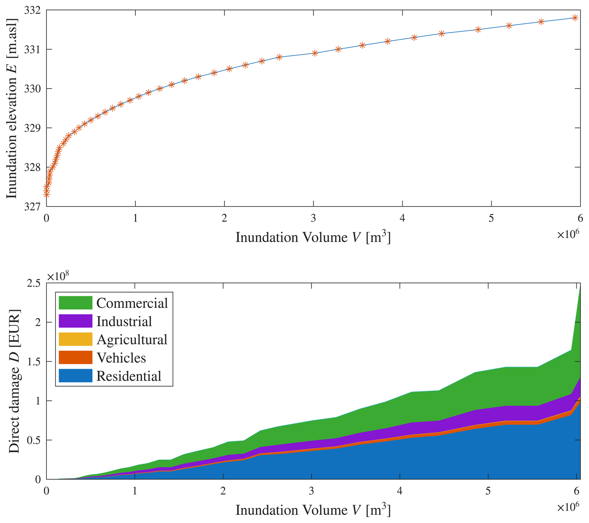
Figure 9 Relation between volume and elevation (upper) and volume and damage (lower) of dike segment 500 (left river side).

Based on the inundation areas of the river sections derived in the inundation module, damages are additionally estimated for river sections following the approach outlined for dike segments. As a result, every river section is associated with a W–D relation, where W denotes the water level in the river section. Flooding in the river section is treated as deterministic conditional on the maximum water level over all time steps resulting from the probabilistic breach analysis. If the river is bifuricated in the section, the lower, non-zero maximum water level of the two segments of a river section is taken as decisive. All damages, e.g., from river sections and dike segments, are summed up to obtain the total direct damage of the simulation run.

Following a comprehensive literature review (Sieg et al., 2019; Carrera et al., 2014; Olesen et al., 2017; de Bruijn et al., 2015; Pfurtscheller, 2014), business interruption costs are estimated at 30 % of the direct damages. Indirect damages are included by adding another 30 % to these costs. Hence, direct damages are augmented by a total of $\mathrm{1.3}\cdot \mathrm{1.3}=\mathrm{1.69}$. It is generally expected that indirect costs and business interruption expenses increase non-linearly with increasing damages; however, the extent of this relationship remains unclear and is influenced by various factors (Koks et al., 2015). Current methods for the comprehensive quantification of indirect damages and business interruption costs at large scale studies are still inadequate (Merz et al., 2010b), justifying the choice to employ two constant factors. Intangible damages are quantified in non-monetary terms, considering factors such as fatalities, natural reserves, critical infrastructure and drinking water protected areas. The reduction of risk associated with these factors is communicated as an additional quantitative benefit of the measures implemented, but it is not included in the formal benefit-cost analysis.

3.6 Model Implementation

The developed flood risk model differs from other methodologies, such as those presented by Vorogushyn (2008) and Domeneghetti et al. (2013), primarily in that the flood simulation model is executed without runtime-coupling with computationally expensive hydraulic and hydrodynamic simulations. This approach enhances computational efficiency while explicitly modeling the effects of the flood process components and their interactions, as is necessary to address the challenges outlines in the introduction. This also enables its incorporation into a comprehensive uncertainty analysis framework, as outlined in the next section. The computational cost of the flood simulation model is on average 0.76 seconds per run (8-thread, 2.8 GHz CPU, no explicit parallelization). This cost scales approximately linearly with the number of breaches. A schematic representation of the model's architecture, implemented in a Matlab environment, is provided in Fig. 10, illustrating the workflow that is executed during each simulation run.

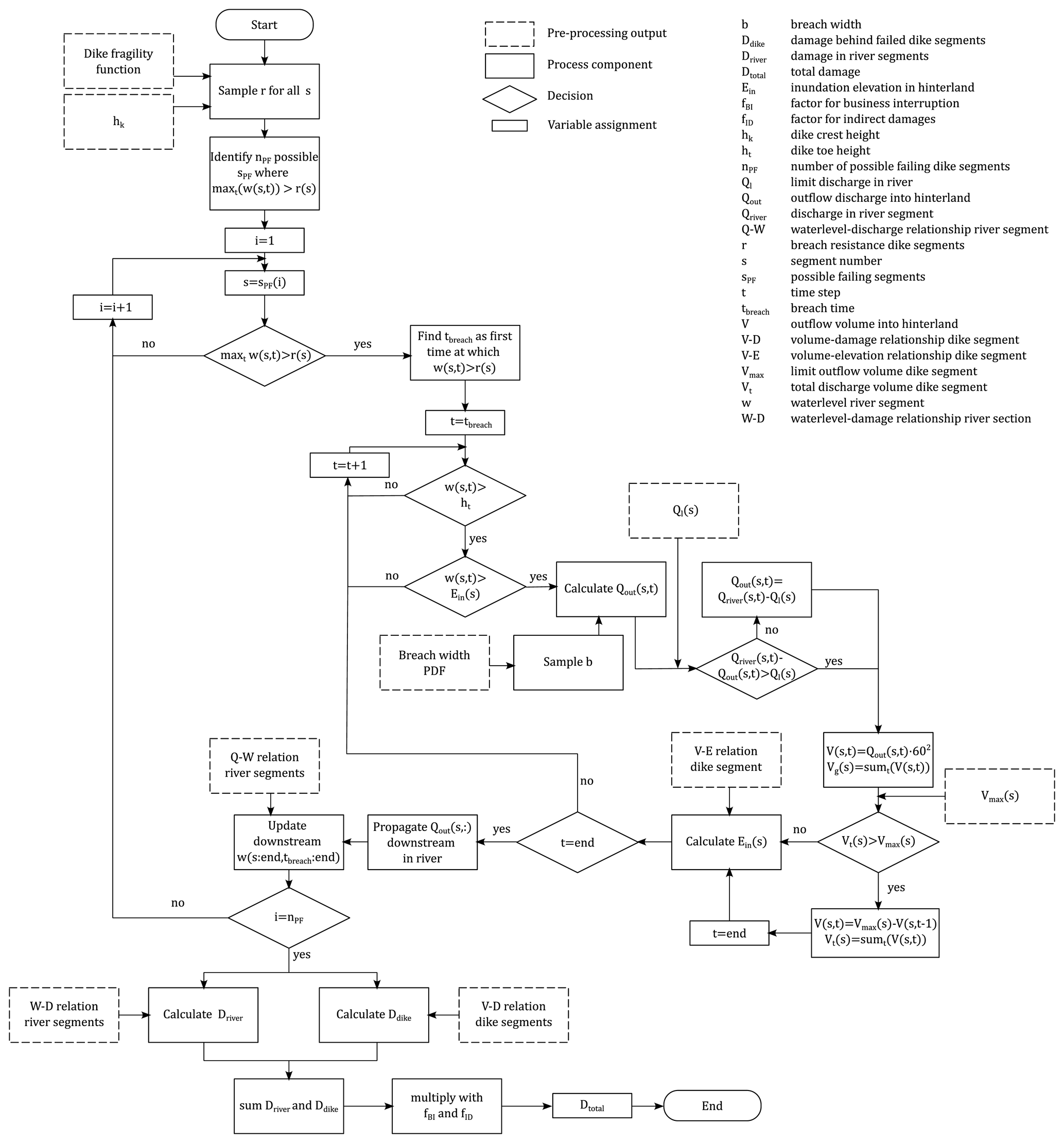
Figure 10 Process diagram of flood simulation model. Schematically shown is the procedure for one Monte Carlo run.

4 Uncertainty modeling

Generally, uncertainties can be categorized into two types: aleatory and epistemic (Hall and Solomatine, 2008). Aleatory uncertainties refer to the inherent natural variability or randomness within the flood process that cannot be reduced by the modeler. By contrast, epistemic uncertainties denote the uncertainties associated with the model and its input data, which can potentially be reduced. Thus, it is imperative, especially within a decision-making context, to quantify the impact of epistemic model uncertainties on the relevant decision parameter(s). For that purpose, the flood risk model is embedded in a 2-level Monte Carlo framework.

4.1 2-level Monte Carlo framework

In the following, Y=𝒴(X) denotes the outcome of the flood simulation model, i.e., the damage estimate associated with a single flood event, with aleatory and epistemic uncertain input parameters $\mathbf{X}=[{\mathbf{X}}_{\mathrm{a}},{\mathbf{X}}_{\mathrm{e}}]$, which are modeled as random variables. X_a contains aleatory random variables, representing the natural variability in flood events, dike resistances and breach widths of failed dike segments. Given the large number of dike segments (≈500) and consequently aleatory random variables, together with the strong nonlinearity of the model response with respect to X_a, the conditional expectation of the damage given X_e is estimated via a first-level Monte Carlo simulation with $n_{{\mathrm{MC}}_{\mathrm{a}}}=\mathrm{3600}$ samples:

$$\begin{array}{}\text{(13)}& \begin{array}{rl}{\mathcal{Y}}_{\mathrm{e}}({\mathbf{X}}_{\mathrm{e}}={\mathbf{x}}_{\mathrm{e}})& ={\mathbb{E}}_{{\mathbf{X}}_{\mathrm{a}}|{\mathbf{X}}_{\mathrm{e}}={\mathbf{x}}_{\mathrm{e}}}\left[\mathcal{Y}\left([{\mathbf{X}}_{\mathrm{e}}={\mathbf{x}}_{\mathrm{e}},{\mathbf{X}}_{\mathrm{a}}]\right)\right]\\ & \approx {\displaystyle \frac{\mathrm{1}}{n_{{\mathrm{MC}}_{\mathrm{a}}}}}\sum _{j=\mathrm{1}}^{n_{{\mathrm{MC}}_{\mathrm{a}}}}\mathcal{Y}\left({\mathbf{X}}_{\mathrm{e}}={\mathbf{x}}_{\mathrm{e}},{\mathbf{x}}_{\mathrm{a}}^{\left(j\right)}\right),\end{array}\end{array}$$

Table 1 Quantified uncertain parameters and their first order Sobol' indices.

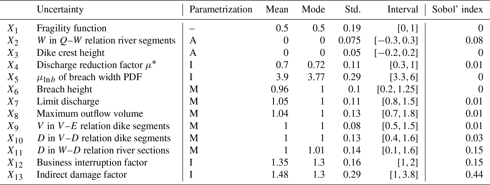
The epistemic uncertainty is represented by 13 random variables X_e, listed in Table 1. They are modeled by beta distributions and incorporated through a second-level Monte Carlo analysis with $n_{{\mathrm{MC}}_{\mathrm{e}}}=\mathrm{200}$ samples. For each quasi-random realization of X_e, the first-level analysis is performed. The expected damage over all simulation runs is estimated as:

$$\begin{array}{}\text{(14)}& \begin{array}{rl}{\mathbb{E}}_{\mathbf{X}}\left[\mathcal{Y}\right(\mathbf{X}\left)\right]& ={\mathbb{E}}_{{\mathbf{X}}_{\mathrm{e}}}\left[{\mathcal{Y}}_{\mathrm{e}}\left({\mathbf{X}}_{\mathrm{e}}\right)\right]\\ & \approx {\displaystyle \frac{\mathrm{1}}{n_{{\mathrm{MC}}_{\mathrm{e}}}}}\sum _{k=\mathrm{1}}^{n_{{\mathrm{MC}}_{\mathrm{e}}}}{\mathcal{Y}}_{\mathrm{e}}\left({\mathbf{x}}_{\mathrm{e}}^{\left(k\right)}\right).\end{array}\end{array}$$

The separation of aleatory and epistemic uncertainties is described in more detail in Straub et al. (2025).

4.2 Risk and benefit estimation

Ultimately, the flood risk model is developed to quantify the expected benefit of implementing individual or combined mitigation measures. The risk reduction associated with a measure M is defined as

$$\begin{array}{}\text{(15)}& \mathrm{\Delta }r\left(a_M\right)=r\left(a_{\mathrm{0}}\right)-r\left(a_M\right)\end{array}$$

where a denotes a decision variable: a₀ represents the baseline scenario without additional mitigation, and a_M corresponds to the implementation of measure M. The annual flood risk under decision a, r(a), is computed as

$$\begin{array}{}\text{(16)}& r\left(a\right)=\mathit{\lambda }\cdot {\mathbb{E}}_{\mathbf{X}}\left[\mathcal{Y}(\mathbf{X},a)\right],\end{array}$$

We reiterate that $\mathit{\lambda }=\mathrm{72}/\mathrm{3500}$ yr⁻¹ is the rate of flood events. The benefit B(a_M) is defined as the sum of the discounted annual risk reduction Δr(a_M) over the operational lifetime of the measure t_o

$$\begin{array}{}\text{(17)}& B\left(a_M\right)=\mathrm{\Delta }r\left(a_M\right)\cdot {\displaystyle \frac{\mathrm{1}-(\mathrm{1}+r_{\mathrm{d}}{)}^{-t_{\mathrm{o}}}}{r_{\mathrm{d}}}},\end{array}$$

with r_d the annual discount rate. Based on the damage samples Y=𝒴(X) resulting from the MC-based flood simulation, a loss exceedance curve can be derived. Therefore, the samples are ordered based on their damage estimate $Y_{\mathrm{1}}\ge Y_{\mathrm{2}}\ge \mathrm{\dots }\ge Y_{n_{{\mathrm{MC}}_{\mathrm{a}}}}$. The exceedance probability of each damage Y_i is calculated as

$$\begin{array}{}\text{(18)}& P(Y\ge Y_i)=i\cdot {\displaystyle \frac{\mathrm{72}}{\mathrm{3500}\cdot n_{{\mathrm{MC}}_{\mathrm{a}}}}}\end{array}$$

This is shown in Fig. 12 for a₀, no measure, and the implementation of the measure under study, a_M. The area in between the two curves corresponds to the expected annual risk reduction in Eq. (15) (Arnel, 1989). To calculate the benefit-cost ratio of a measure, the benefit B(a_M) is compared against the sum of discounted costs.

4.3 Sensitivity analysis

Sensitivity analysis aims at explaining how variations in model outputs can be attributed to uncertainties in input parameters (Pianosi et al., 2016). In this study, first-order Sobol' indices are calculated as a byproduct of the uncertainty analysis. They offer insights into the relative importance of parameter uncertainties, calculated as the direct contribution of each input parameter to the output variance

$$\begin{array}{}\text{(19)}& S_{X_{\mathrm{e},i}}={\displaystyle \frac{\mathrm{Var}\left(\mathbb{E}\right[Y_{\mathrm{e}}\left|X_{\mathrm{e},i}\right])}{\mathrm{Var}\left(Y_{\mathrm{e}}\right)}}.\end{array}$$

Since aleatory uncertainty cannot be reduced, quantifying the sensitivity with respect to all uncertainties $\mathbf{X}=[{\mathbf{X}}_{\mathrm{a}},{\mathbf{X}}_{\mathrm{e}}]$ is not expedient, especially in a decision making context. Therefore, the sensitivity analysis considers as input only the epistemic uncertainties X_e and as output the expected value of 𝒴(X,a) with respect to the aleatory uncertainties X_a, $Y_{\mathrm{e}}={\mathcal{Y}}_{\mathrm{e}}({\mathbf{X}}_{\mathrm{e}}={\mathbf{x}}_{\mathrm{e}})$, estimated in Eq. (13). To approximate $\mathbb{E}\left[Y_{\mathrm{e}}\right|X_{\mathrm{e},i}]$ the samples are partitioned into five bins of equal width over the range of X_e,i, and the mean of Y_e within each bin is used as an estimate of the conditional expectation. If the absolute influence of parameter uncertainties on a specific decision is of interest, the expected value of partial perfect information (EVPPI) (Straub et al., 2025) is a more suitable metric. EVPPI quantifies the expected monetary benefit of making an improved decision when perfect information about a specific uncertain input X_e is available. It can be used to assess whether it is worthwhile to invest in reducing uncertainty in a particular input parameter, or to identify which uncertainties should be prioritized in further analysis or data collection.

5 Exemplary results

In this section, we illustrate selected applications of the developed flood risk model. To this end, it is applied to the Bavarian Danube with the objective of assessing the cost-effectiveness of the controlled detention basin introduced in Sect. 2. The results of the case study are still confidential due to ongoing work on the climate inputs and the pending publication of the study. Consequently, the preliminary estimates of the detention basin's benefits shown in Fig. 13 are presented without numerical values. In this study, a total of $n_{\mathrm{MC}}=n_{{\mathrm{MC}}_{\mathrm{a}}}\cdot n_{{\mathrm{MC}}_{\mathrm{e}}}=\mathrm{3600}\cdot \mathrm{200}=\mathrm{720}\mathrm{000}$ Monte Carlo simulation runs are performed. The samples are used to derive the expected loss exceedance curve of events T>100 years at the Bavarian Danube, shown in blue in Fig. 11. The sampling process follows the 2-level framework outlined in Sect. 4.1, that enables the distinction between the influence of aleatory and epistemic uncertainties. The impact of epistemic uncertainties is represented by the shaded areas in Fig. 11, which correspond to the 90 % quantile. Five loss exceedance curves, selected randomly from the n_E=200 second-order simulation runs, are depicted in black to illustrate the effect of epistemic model uncertainties. As apparent from Fig. 11, the influence of model uncertainties is more pronounced for larger, less frequent damage events.

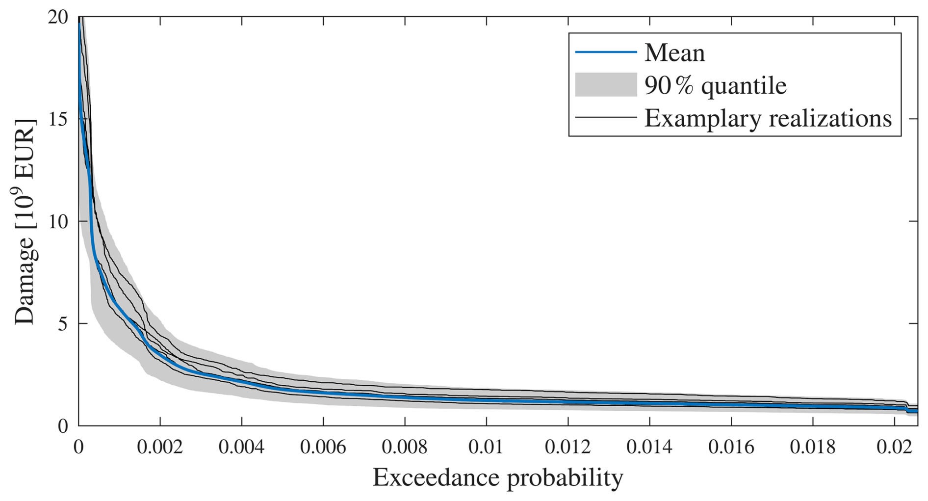
Figure 11 Loss exceedance curve for events with T>100 at at least one location at Bavarian Danube. Mean (blue), 90 % quantile (grey) and five randomly selected loss exceedance curves given fixed epistemic parameters.

The developed flood risk model is further applied to quantify the flood risk reduction potential Δr(a_M) of a controlled detention basin located near Riedensheim at the Bavarian Danube, introduced in Sect. 2. For this purpose, the preliminary loss exceedance curve given events with T>100 years is derived with (blue) and without (red) the detention basin, shown in Fig. 12. As outlined in Sect. 4.2, the annual risk reduction is equivalent to the area between the two loss exceedance curves. We note that the uncertainties in the loss exceedance curves are large relative to the difference in the mean estimates. However, the two curves are highly correlated, because most uncertainties affect the damages with and without the measure in the same way. Due to this correlation, the uncertainty in the risk reduction (the benefit of the measure), also depicted in Fig. 13, is much smaller than might be expected by looking at Fig. 11. The coefficient of variation of the risk reduction is 25 %.

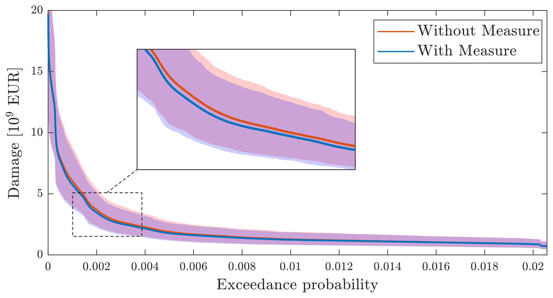
Figure 12 Loss exceedance curve for events with T>100 at at least one location at Bavarian Danube with (blue) and without (red) mitigation measure. Respective 90 % quantile shown as shaded area.

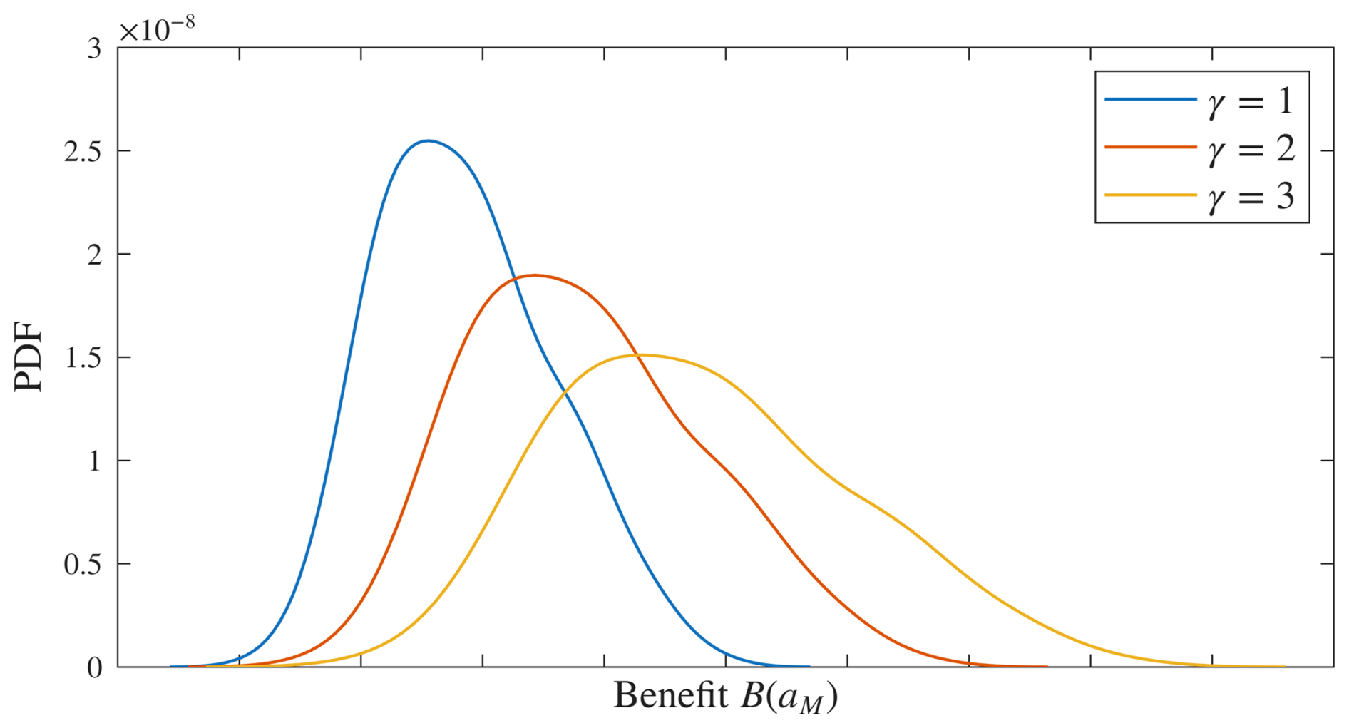
Figure 13 Probability distribution (PDF) of benefit B(a_M) at the Bavarian Danube achieved by the detention basin. The blue PDF corresponds to the assumption of a constant climate, the red PDF to a linear increase in flood frequency until 2120 by a factor γ=2 and the yellow PDF to an flood frequency increase by a factor of γ=3. No numbers are shown on the x-axis due to confidentiality of the results.

Kernel-smoothing is applied to estimate the probability density function (PDF) of the benefit B(a_M) (discounted total risk reduction), which is depicted in blue in Fig. 13. No numerical values are provided as the results are preliminary. To incorporate these results into a benefit-cost analysis, the expected annual flood risk reduction over the projected lifetime of the measure is discounted relative to the reference year, summed, and compared to the discounted costs of the measure, as described in Sect. 4.2. Analogously, multiple mitigation measures can be incorporated into the model, allowing for comparison of the benefits of different combinations.

A total of 13 epistemic uncertainties are incorporated into the uncertainty analysis; their parameterizations are summarized in Table 1. While covering key sources, this selection is not exhaustive, as it is not feasible to represent all potential epistemic uncertainties. The selected uncertainties are represented either directly (I), or via additive (A) or multiplicative (M) factors. In the case of the fragility function, the parameterized factor is used to interpolate between the lower and upper uncertainty bounds shown in Fig. 5. All factors are modeled using beta distributions, as illustrated in Fig. 14. The annual risk with respect to the aleatory uncertainties, $\mathit{\lambda }\cdot {\mathbb{E}}_{{\mathbf{X}}_{\mathrm{a}}|{\mathbf{X}}_{\mathrm{e}}={\mathbf{x}}_{\mathrm{e}}}\left[\mathcal{Y}\right([{\mathbf{X}}_{\mathrm{e}}={\mathbf{x}}_{\mathrm{e}},{\mathbf{X}}_{\mathrm{a}}]\left)\right]$, are plotted against the sampled factor values X_i=x_i in the same Figure. The substantial influence of the indirect damage factor on the annual risk is clearly evident. Additionally, a formal variance-based sensitivity analysis is conducted, and the first-order Sobol' indices are provided in Table 1.

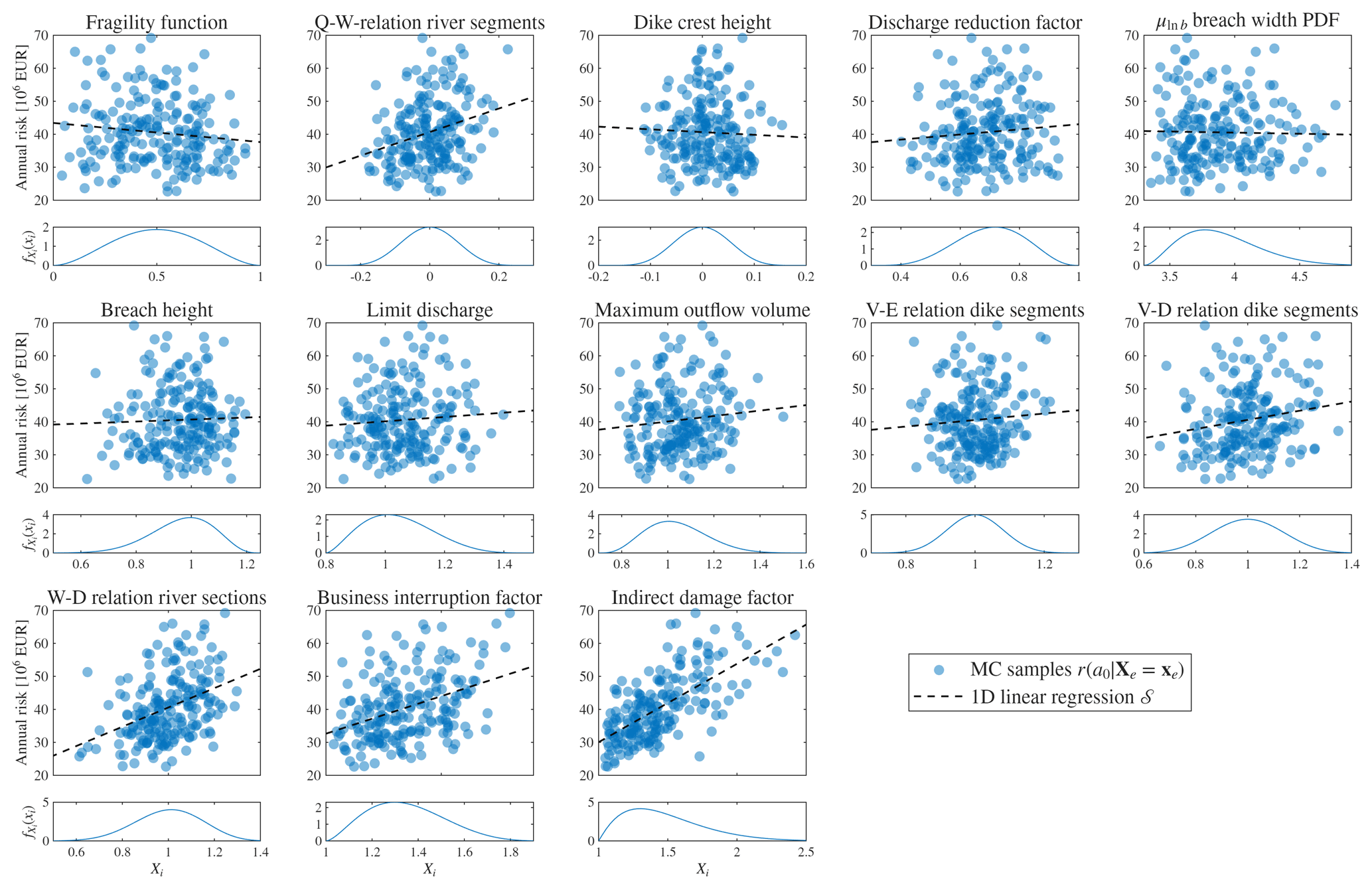
Figure 14 Scatter plot of the influence of considered epistemic uncertain parameters on the annual risk, a fitted 1D linear regression 𝒮_i, and assigned underlying beta distribution of X_i.

The results of the sensitivity analysis suggest that the uncertainty of parameters entering the damage module (X₁₀–X₁₃) has the greatest impact on the annual flood risk. This finding supports the conclusions of Apel et al. (2009a), who noticed that the choice of the flood damage model has a more significant impact on the flood risk estimate than the parameters within the other flood process models, emphasizing the need for further development of the damage module. Furthermore, the uncertainty in the damage estimates for river sections appears to dominate those for dike segments, suggesting the need for further examination and development of this part of the model. The uncertainties inherent in the hydrological load module are not incorporated in this uncertainty analysis. To assess the impact of a possible climate-change-based increase in flood frequency on the risk reduction potential of the measure, an empirical scenario analysis is conducted. The occurrence rate of a flood $\mathit{\lambda }=\mathrm{72}/\mathrm{3500}$ yr⁻¹ is linearly increased until the year 2120 by a factor γ, such that the updated, time-dependent occurrence rate is calculated as

$$\begin{array}{}\text{(20)}& {\widehat{\mathit{\lambda }}}_{\mathit{\gamma }}\left(t\right)={\displaystyle \frac{\mathit{\gamma }-\mathrm{1}}{t_{\mathrm{o}}}}\cdot t\cdot \mathit{\lambda }+\mathit{\lambda }\mathrm{for}t\in [\mathrm{0},t_{\mathrm{o}}]\end{array}$$

The influence of γ on the distribution of annual flood risk reduction is illustrated in Fig. 13 for the two scenarios γ=2 and γ=3. An increased flood occurrence rate leads to larger expected flood risk reduction, and consequently higher benefit of the detention basin; however, it also results in increased uncertainty.

6 Concluding remarks

This work proposes a flood risk model to enable large-scale uncertainty-aware flood risk assessments for decision support on mitigation measures. The model is computationally efficient because it makes use of the results of different climatic, hydrodynamic and hydraulic simulations conducted in a pre-processing step. As a result, it does not depend on computationally intensive simulations during run time. A key element enabling this independence is the developed flood routing method, along with segment-specific lookup tables that store the relationships between inundation elevation, floodwater volume, and damages. This computational efficiency allows the model to be integrated into a two-level Monte Carlo framework for uncertainty quantification. Within this framework, different types of uncertainty – aleatory and epistemic – are treated separately. This separation allows for the isolated examination of epistemic uncertainties, helping to understand the influence of various model uncertainties and make targeted improvements. Furthermore, the separation ensures that the estimated benefits of mitigation measures remain robust across a wide range of possible flood events and failure scenarios. Especially in the context of natural hazards like floods, which are characterized by high aleatory uncertainty, it is essential to quantify, communicate, and incorporate this uncertainty into the decision-making process.

The literature review in Sect. 1 highlighted the inherent trade-offs in flood risk models between process representation, spatial coverage, and the integration within uncertainty analyses. The developed model enables both large-scale flood risk and benefit assessments as well as detailed uncertainty analyses. However, a compromise is made through simplifications that are necessary to allow pre-processing of parts of the model, which reduces the model’s accuracy locally. Nevertheless, results of module verification and the uncertainty analysis suggest that the effect of these inaccuracies remains within an acceptable range, in particular when considering mitigation measures that act globally, such as flood detention basins. Notably, the results of the sensitivity analysis indicate that the annual flood risk is highly sensitive to the uncertainty in the damage module, such that future improvements should focus on components of the damage module. As long as the current uncertainties in damage estimation prevail, investments towards improving the other components of the flood risk model seem to be unjustified.

The flood risk model is applied to the 380 km of Bavarian Danube in Germany to assess the potential risk reduction of mitigation measures. Computational time scales approximately linearly with the number of dike segments; an extension of the model to the entire Danube, which spans roughly 2850 km across ten countries, is thus expected to increase runtime by no more than a factor of ten. On this basis, we argue that the model can be applied in large-scale studies and support increasing system thinking. More critical for large cross-border applications are the pre-processing steps, which entail acquiring the necessary data, models and large-scale simulation outputs from multiple stakeholders. We acknowledge that this can be challenging in practice, but this challenge will be faced by any modeling approach. The extent to which uncertainties propagate and accumulate downstream over such long river stretches would require careful examination. Applying the model to an entirely new study area follows a similar process, provided that region-specific climatic, hydrological, and hydraulic simulation models are available. The pre-processing steps are repeated to capture relevant regional characteristics.

To further support system thinking, the model can be extended to include the entire catchment, rather than representing only the main river. Although tributary contributions are accounted for in the flood scenarios, potential protection failures, local mitigation measures, and other dynamic effects along tributaries are not explicitly modeled; this limitation should be addressed in future work. Explicitly modeling tributaries in the same manner as the main river is straightforward and, if implemented with efficient parallelization, would not substantially increase computational cost. Such an extension would enable catchment-wide optimization of mitigation measures and improve the accuracy of risk estimates.

A further limitation of the model is due to the hydrological simulation of catchment runoff, which is performed during pre-processing in the hydrological load module. While the implemented design choice permits short run times of the main flood simulation module, it does not allow the assessment of interventions influencing the hydrological flood-forming processes. Consequently, many nature-based solutions cannot be evaluated using the present model implementation.

In contrast to process-based approaches (Sairam et al., 2021), flood dynamics are not explicitly represented in the model. Consequently, parameters such as flow velocity and inundation duration are not accounted for in the damage estimation, which limits predictive accuracy and introduces additional uncertainty. However, these uncertainties are implicitly captured within the 2-level framework. For applications to mitigation measures that act locally, the modular structure of the framework allows the integration of high-resolution 2D hydraulic simulations and more detailed damage models for the affected areas.

Notwithstanding its limitations, the developed model provides a solid foundation for decision-making, such as in benefit-cost analyses. We argue that the proper assessment of the uncertainty, which is enabled by the developed model, is more important for decision-making than the limitations required to enable this assessment. The practicality of the model is demonstrated in a real-world application to flood mitigation at the Bavarian Danube. Therein, the benefit of a flood mitigation measure, along with its associated uncertainties, is quantified. In the future, the model can support assessments of various mitigation strategies, help identify high-risk areas, or optimize the combination of mitigation measures. In this way, we demonstrate how dynamic, probabilistic, and integrated flood risk management can be implemented in practice. We hope that our work encourages and supports decision-makers in moving toward a more holistic approach to flood risk management.