Bayesian forecasting of triggered landslides

We present a Bayesian probabilistic framework for landslide forecasting, explicitly accounting for the sources of epistemic uncertainty that affect landslide occurrence. The method describes the probability of landslide occurrence as a distribution, rather than a single value, allowing a more realistic treatment of uncertainty arising from incomplete landslide inventories, variable measurements, and the inherent complexity of landslide processes. We apply the probabilistic framework to a 22-year dataset of shallow landslides and daily rainfall records from the Campania region (southern Italy). Each landslide is associated with the nearest rain gauge, and forecasts are computed within Thiessen polygons representing the area of influence of each rain gauge. Posterior landslide probabilities are calculated for different daily rainfall thresholds using Bayes' theorem, with prior and likelihood terms modelled as uniform and Beta distributions, respectively. Results show that posterior probabilities increase progressively with rainfall, ranging from 0 to 10⁻³ at the lowest threshold (0.2 mm) to up to 10⁻¹ at the highest threshold (70 mm) when uncertainty is not considered, and from 10⁻³ to values between 0.2 and 0.8 at the highest threshold (70 mm) when uncertainty is accounted for, and no sharp physical threshold emerges. The retrospective forecast skill improves with rainfall information, as demonstrated by consistent gains in posterior over prior probabilities. This gradual increase in probability, without the emergence of a sharp physical threshold, supports the use of probabilistic rather than deterministic approaches for landslide forecasting in operational contexts. The proposed Bayesian probabilistic framework is designed to be generalizable to other triggering mechanism (e.g., earthquakes) and potentially adaptable to other regions, provided that sufficient data are available. Although the method is data-intensive, it enables transparent, uncertainty-informed forecasts, with potential applications in early warning systems and risk management strategies. Future developments may include the incorporation of antecedent rainfall and geological conditioning factors across broader spatial and temporal scales.

1 Introduction

Predicting the occurrence of future landslides is a key scientific component for planning effective risk management measures. In common practice, this goal is often addressed using heuristic or statistical thresholds based on triggering phenomena, such as exceedance of rainfall threshold levels (Crosta and Frattini, 2000; Guzzetti et al., 2007; Segoni et al., 2018). These approaches typically lead to deterministic (i.e., dichotomic, binary) statements (e.g., landslide occurrence versus non-occurrence), thereby simplifying – at least in principle – decision-making.

In contrast, a probabilistic landslide forecasting provides an explicit estimate of the probability of occurrence, together with a quantitative representation of uncertainty (Bean, 2000). We argue that this constitutes a more suitable framework for landslide forecast. Probabilistic approaches can explicitly account for the ubiquitous/pervasive uncertainties inherent in the landslide processes, which arise from complex interactions among multiple nonlinearly coupled variables (e.g., rainfall, soil strength, water content, permeability, slope, soil type). These uncertainties stem from various sources, including incomplete data on rainfall and landslide occurrence (location and timing), limited knowledge of soil properties, measurement accuracy and errors, spatial and temporal variability of model parameters, and the simplifying assumptions embedded in the modelling approaches. As a result, deterministic (dichotomic, binary) predictions are inherently challenging, particularly for forecasting horizons longer than a few tens of hours.

To address these limitations, Bayesian inference has been applied to estimate minimum rainfall conditions sufficient for landslide initiation e.g., through rainfall thresholds (Guzzetti et al., 2007, 2008; Brunetti et al., 2010). Scholars have proposed probabilistic frameworks that incorporate uncertainty in rainfall thresholds, quantifying the probability of landslide occurrence conditional on rainfall metrics (Berti et al., 2012; Pecoraro and Calvello, 2021; Jiang et al., 2022; Zhao et al., 2025). Zhang et al. (2025) further proposed a Bayesian framework to define probabilistic thresholds using rainfall variables automatically extracted from rainfall time-series.

Most existing probabilistic approaches to landslide forecasting still rely on the concept of rainfall thresholds, treating uncertainty primarily as variability around the threshold parameters themselves; for instance, through confidence intervals on intensity-duration curves or through non-exceedance probability levels (Peruccacci et al., 2017; Rossi et al., 2017). While such approaches represent a meaningful step beyond purely deterministic methods, the available landslide hazard modelling frameworks rarely address a thorough quantification of uncertainty, and uncertainty in rainfall datasets and landslide inventories is known to degrade the reliability of threshold estimates (Peres et al., 2018). In this sense, the probabilistic content of these frameworks is largely restricted to uncertainty about the threshold, rather than a fundamental reconceptualization of landslide triggering as an inherently probabilistic process (Felsberg et al., 2023). However, most existing probabilistic frameworks yield point-valued probability estimates and assume a priori the existence of a sharp physical boundary separating triggering from non-triggering conditions.

A further complication is the definition and sampling of non-triggering rainfall conditions. In real-world datasets, rainfall events that do not trigger landslides are far more common than those that do, resulting in highly imbalanced datasets, particularly in regions where data are sparse. The choice of how to sample non-events is therefore not a neutral methodological decision: it directly shapes the estimated probability of landslide occurrence and can introduce substantial bias into early warning systems (Peres and Cancelliere, 2014; Peres et al., 2018).

More generally, data-driven learning techniques have increasingly been adopted to estimate landslide probability in both space and time (Lombardo et al., 2020; Mondini et al., 2023) combining prior knowledge and observations within probabilistic frameworks that explicitly account for uncertainty. Although machine-learning approaches have shown promising predictive capabilities, they often require large training datasets, may suffer from limited interpretability, and do not always provide an explicit characterization of epistemic uncertainty (Chen et al., 2025).

Addressing these gaps requires a framework that treats landslide probability not as a function of threshold exceedance, but as a distribution that reflects the current state of knowledge given the available evidence.

Here, we present a formal probabilistic framework that incorporates the natural variability and uncertainties in landslide occurrence and triggering factors. The proposed framework addresses epistemic uncertainty arising from incomplete observations, measurement limitations, and imperfect knowledge of landslide-triggering processes. Our approach does not assume the existence of a physical threshold and, instead, allows landslide probability to be estimated as a function of the relevant triggering conditions. To illustrate the method, we apply the probabilistic framework to rain-triggered landslides in Campania region, Italy.

2 Study area

The study area is located in western Campania, Southern Italy, and consists of two sub-areas, the Sarno and Lattari mountain ranges in the mainland and the Ischia Island in the Tyrrhenian Sea (Fig. 1).

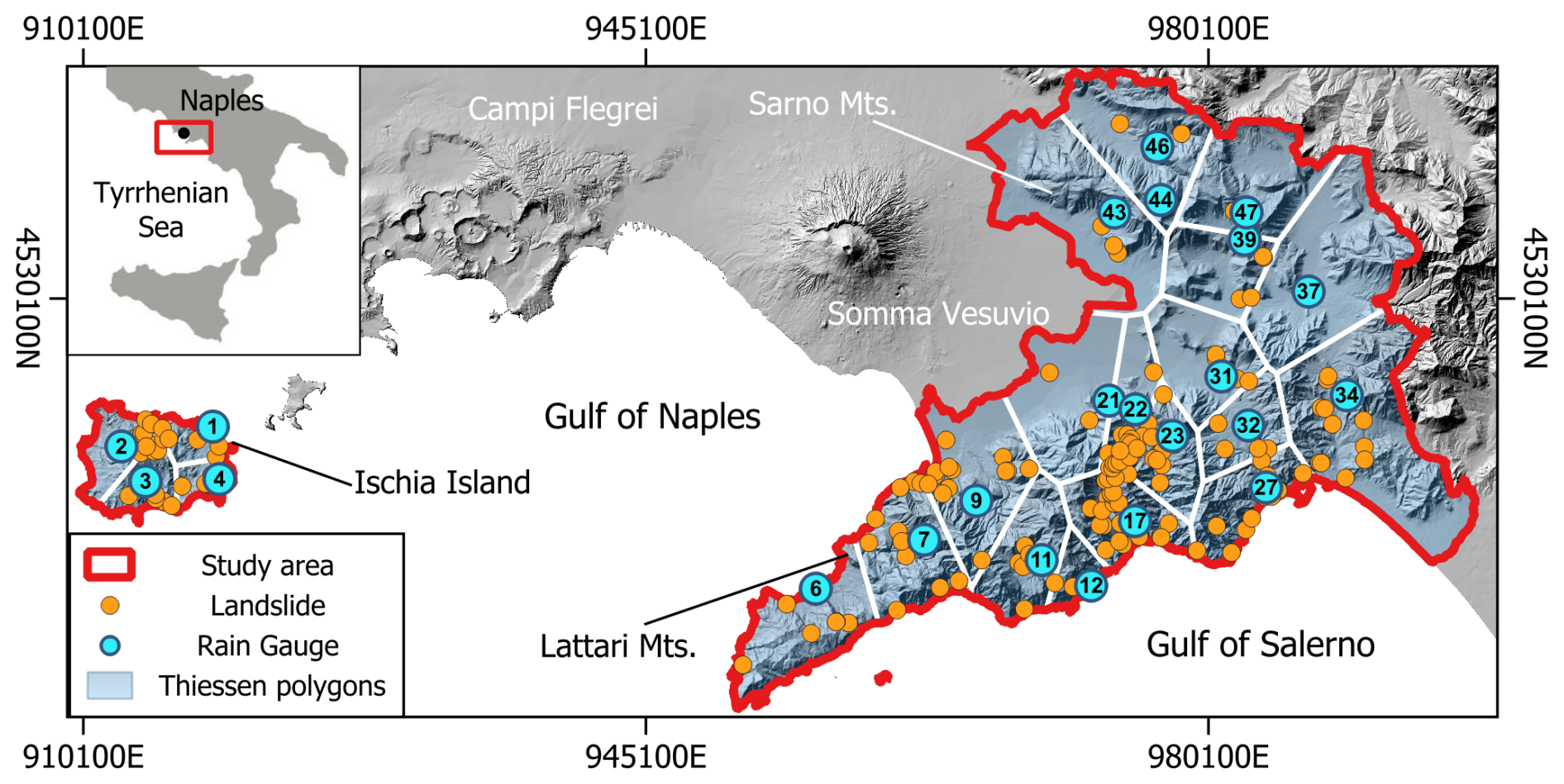
Figure 1 Study area (highlighted in red) encompasses the Sarno and the Lattari mountain ranges and the Ischia Island. Top-left panel shows location of the study area in southern Italy. Main map shows location of 169 landslides (orange dots, see Table A1 for more information on the landslide catalogue) and 23 rain gauges (blue dots) taken from the Centro Funzionale Multirischi, Campania Region (https://centrofunzionale.regione.campania.it/#/pages/dashboard, last access: 31 March 2024). See Table 1 for details on the rain gauges. Thiessen polygons (rain gauges areas of influence) are shown in light blue.

In the Sarno and Lattari ranges crop out carbonate rocks, Jurassic to Cretaceous in age, in a NW-dipping monoclinal setting locally cut by normal faults and thrusts (De Vita et al., 2013; Forte et al., 2019). Volcaniclastic sediments resulting from multiple eruptions of the Somma Vesuvio, Campi Flegrei, and Epomeo volcanoes mantle the study area. The volcaniclastic deposits are spatially highly discontinuous, with maximum thickness of 4 to 7 m in the Sarno range, 2 to 3 m in the Lattari range, and 1 to 2 m in Ischia Island (De Vita et al., 2007). Elevation ranges from sea level to 787 m in the Ischia Island, and from sea level to 1444 m in the Sarno and Lattari ranges, with slopes locally exceeding 45°. Climate is Mediterranean, with distinct dry and wet seasons and a mean annual precipitation in the range from 500 and 1700 mm depending on elevation and distance from the seacoast (Ducci and Tranfaglia, 2008; Longobardi and Boulariah, 2022). Landslides are frequent and abundant in the area and are primely shallow (surficial) failures that involve the volcanic soil cover, giving rise to soil slides and debris flows. Rock falls and topples affect the carbonate and volcanic steep slopes locally (de Riso et al., 2004; Cascini et al., 2008; Fusco et al., 2023).

3 Materials

3.1 Landslide information

Through a literature and archive search, we built a catalogue with information on 317 landslides in the 69-year period 1954–2022, including 169 landslides (53.3 %) in the 23-year period 2000–2022 (Fig. 2). To search for landslide information, we analysed 20 scientific journal articles and conference proceedings, including papers discussing landslide inventories and studies on the instability conditions of single slopes. In addition, we searched 15 online news sources. The landslide information was further integrated using national archives available from the CNR Research Institute for Geo-Hydrological Protection (IRPI, https://www.irpi.cnr.it/, last access: 7 February 2024), which contributed to adding 117 additional landslides to the catalogue (36.9 %).

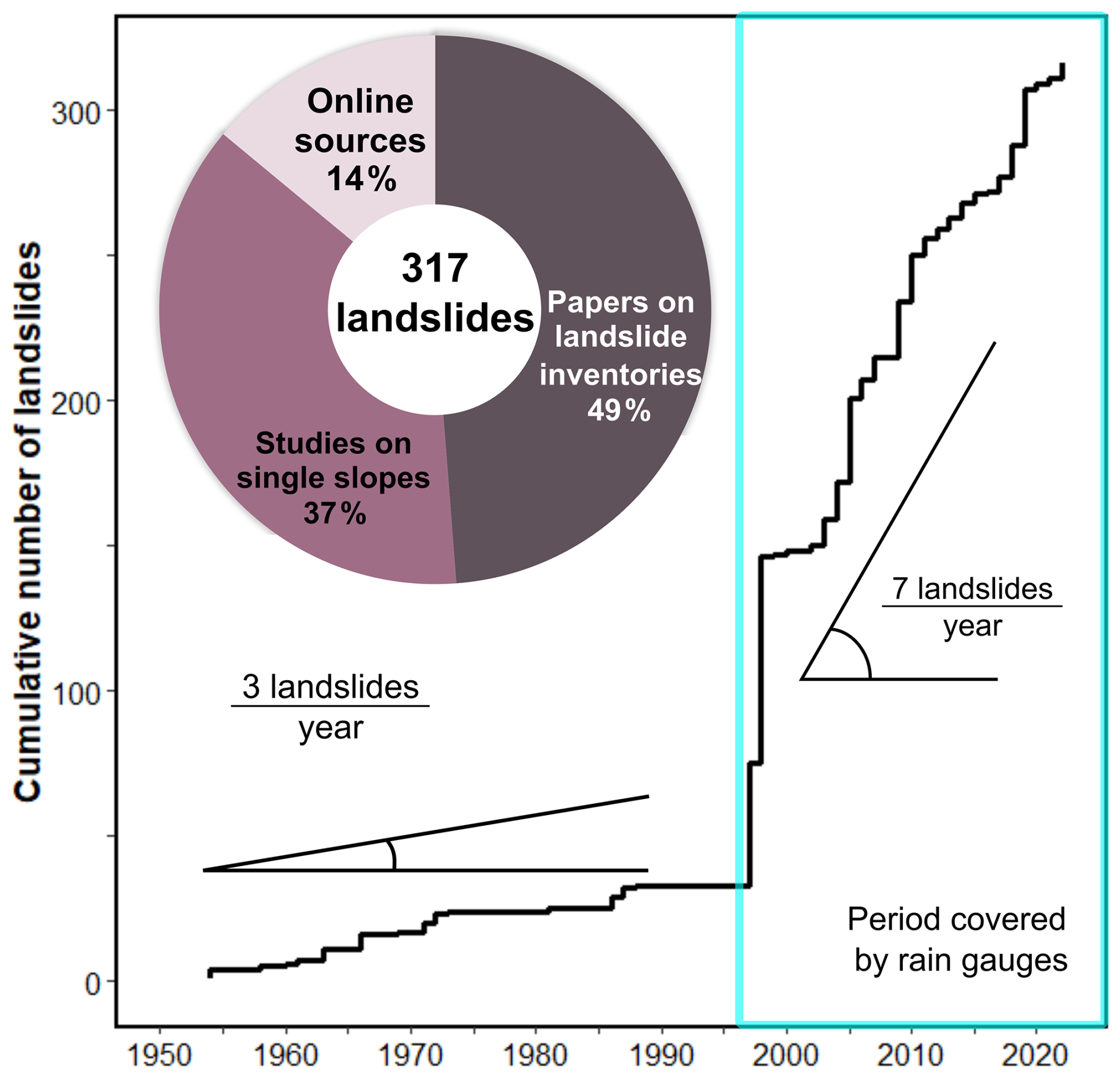
Figure 2 Number of landslides in the catalogue. From 1954 to 2000, the reported number of landslides is 3 per year. After 2000 the reported number of landslides is 7 per year. Pie chart shows percentage of information obtained from different sources used to compile the landslide catalogue.

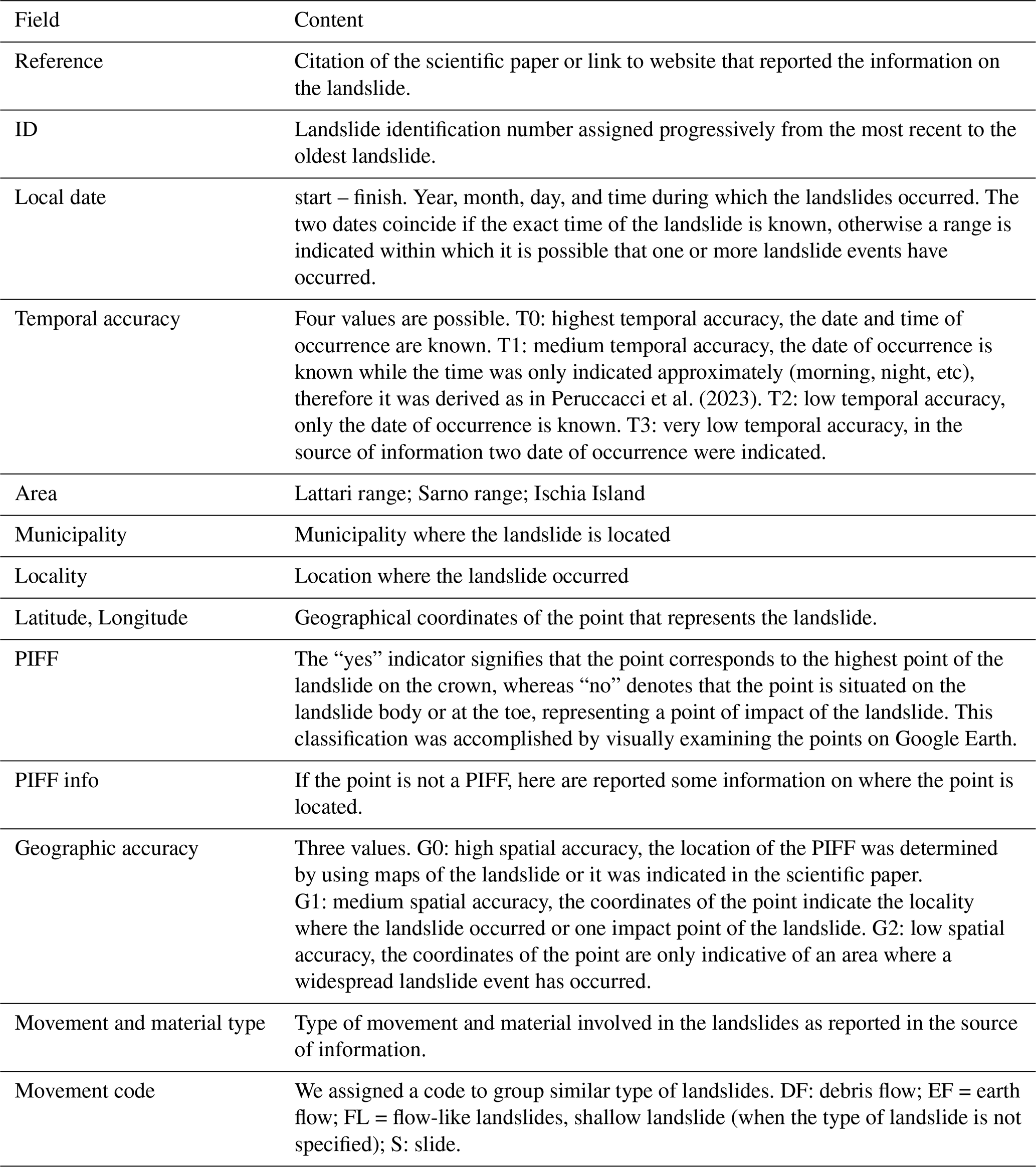
For each landslide, the catalogue lists (i) a unique landslide identification number, (ii) the time or date of occurrence of the failure, (iii) the geographical location, Province, Municipality, and place name of the slope failure, (iv) the landslide type, and (v) the material involved in the failure (see Table A1 for more information on the landslide catalogue). For 98 landslides (30.9 %), the time of failure is available. This set includes 35 events for which the timing is known within a 3 to 6 h window, i.e. the landslide is known to have occurred sometime during that interval, although the precise moment is unknown (Peruccacci et al., 2023). For the remaining 219 landslides (69.1 %) only the date of occurrence is known. In the catalogue, the first and the last landslide for which the failure time is known occurred both in the Ischia Island, on 10 January 2000 at 16:00 LT (local time), and on 26 November 2022 at 12:00 LT. In this 23-year period, the exact or the approximate time of failure is known for 98 landslides (30.9 %).

Figure 2 shows the cumulative number of landslides listed in the catalogue over time. The slope of the cumulative curve, a representation of the rate at which landslides are reported in the catalogue (Guzzetti et al., 2000; Jenkins et al., 2012), shows distinct variations. From 1954 to 2000, the slope of the cumulative curve is low, with less than 150 landslides reported in 45 years, three landslides per year, on average. After 2000, the steeper slope of the cumulative curve reveals an increased rate of seven landslides per year, clustered in short periods i.e., in landslide events (Rossi et al., 2010), of which the event with the largest number of landslides is the 5 May 1998 Sarno event (Del Prete et al., 1998; Calcaterra et al., 1999). Inspection of Fig. 2 shows that after the devastating Sarno event the number of landslides listed in the catalogue increases significantly. After the Sarno event, the cumulative curve shows minor variations in the number of landslides. We attribute the variations to incompleteness of the catalogue (i.e., the rate at which landslides occurred did not change but landslides are reported differently in the catalogue) or to different rainfall conditions (drier/wetter periods) that have triggered different numbers of landslides.

With the available information, it is not possible to discriminate the causes of the different landslide rates. We note that the rate at which landslides are listed in the catalogue represents a lower estimate of the true (and unknown) landslide occurrence rate. The number of landslides that have occurred between 2000 and 2022 is certainly higher than what is listed in the catalogue. Considering the slope of the cumulative curve as a loose proxy for the completeness of the catalogue (Guzzetti et al., 2000; Jenkins et al., 2012), for our modelling we consider the portion of the catalogue from 2000 to 2022 listing 169 landslides (Fig. 2).

Figure 3a shows the monthly distribution of landslides in the catalogue. From 1954 to 1999 (47 years), most (92.5 %) of the reported landslides occurred between January and May. The distinct peak in the number of landslides in May corresponds to the Sarno event, the event with the largest number of landslides in the catalogue. From 2000 to 2022 (23 years), most of the reported landslides (89.3 %) were in autumn and winter, with the largest number of reported failures in November and March.

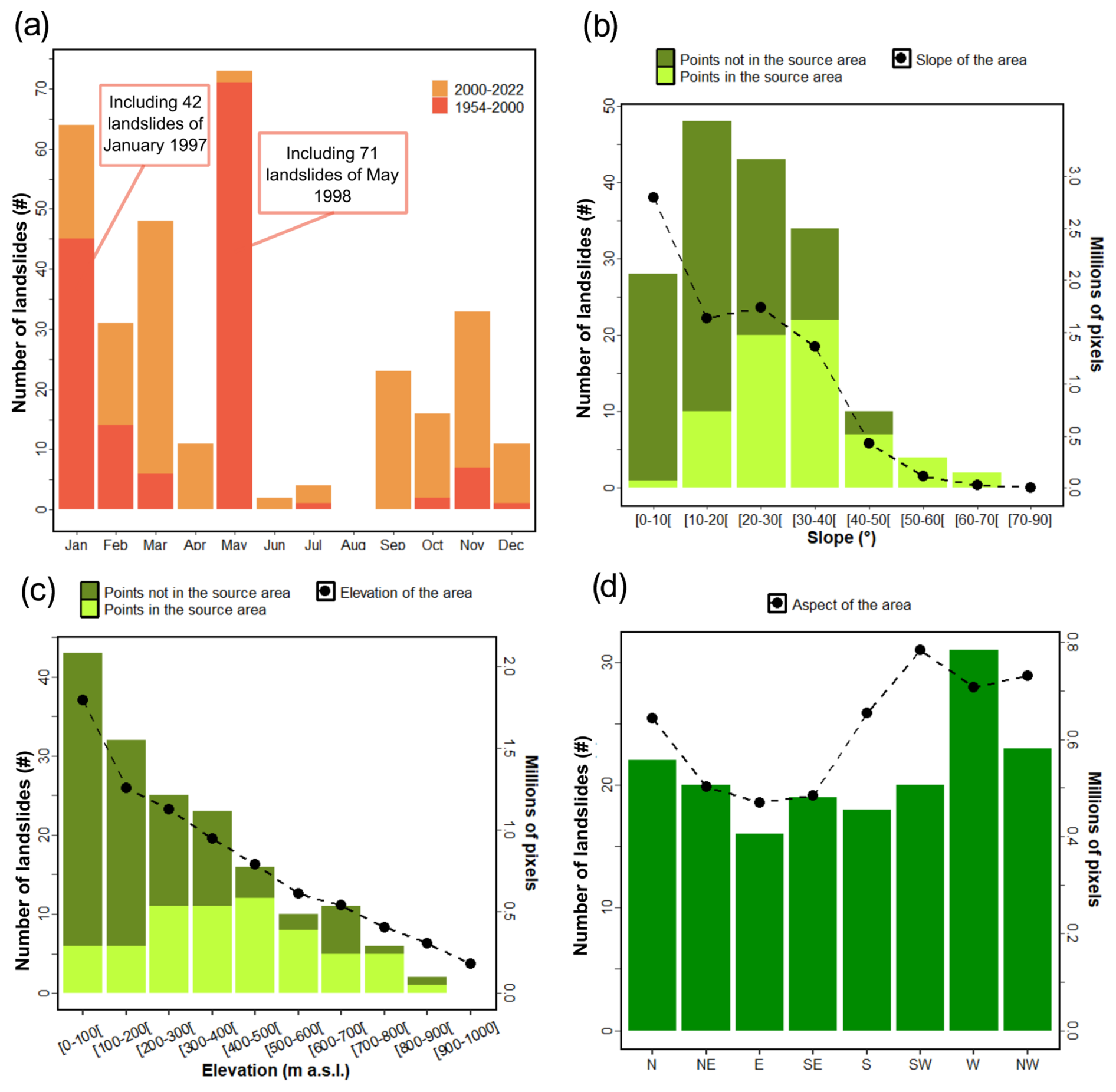
Figure 3 Analysis of the landslide catalogue. (a) Seasonal distribution. Number of landslides recorded for each month over the period 1954–2022. Colours separate landslides within the completeness period. Before 2000, two large landslides events are reported in January 1997 and May 1998. (b) Distribution of terrain slope. (c) Distribution of terrain elevation. Landslides are shown by different colours depending on whether the mapped point falls within or outside the source area. Black dots represent slope/elevation distribution for the entire study area. (d) Distribution of terrain aspect. Black dots show the aspect distribution for the entire study area.

To represent the landslides geographically, each failure in the catalogue is represented by a unique pair of geographical coordinates. Some of the points (39 %) are in the landslide source area whereas others (61 %) are in the landslide deposit or at the landslide toe. For some of the landslides, and particularly for debris flows that have travelled long distances, which are common in the area (Zanchetta et al., 2004; Revellino et al., 2004; Jackob and Hungr, 2005; Nocentini et al., 2015), the distance between the source and the toe areas can be significant (up to 4 km). Of all the points in the landslide source areas, the majority are located on 30 to 40° slopes (Fig. 3b), a range of terrain slope not very abundant in the study area, and in all terrain elevations (Fig. 3c), with a minor peak around 400–500 m. This suggests a control of the terrain slope on landslide initiation, consistent with previous findings that debris flows in the area originate preferentially on 35 to 37° slopes (Guadagno, 1991), and a lack of control of elevation on landslide initiation. Conversely, points located in the landslide deposit or toe are located preferentially on gentler slopes (10–20°) and at elevation below 400 m, and they may be located where the landslides impacted structures or infrastructures, and for this reason were noticed and reported. Regardless of their location – i.e., in the landslide source, deposit, or toe – points are more abundant on N-NW facing slopes (Fig. 3d), possibly because these slopes tend to receive less sun and are more humid, favouring slope instability.

3.2 Rainfall data

We obtained daily rainfall measurements from 23 rain gauges in the study area operated by the Centro Funzionale Multirischi of the Campania Region (Fig. 1, Table 1).

Table 1 Rain gauges information.

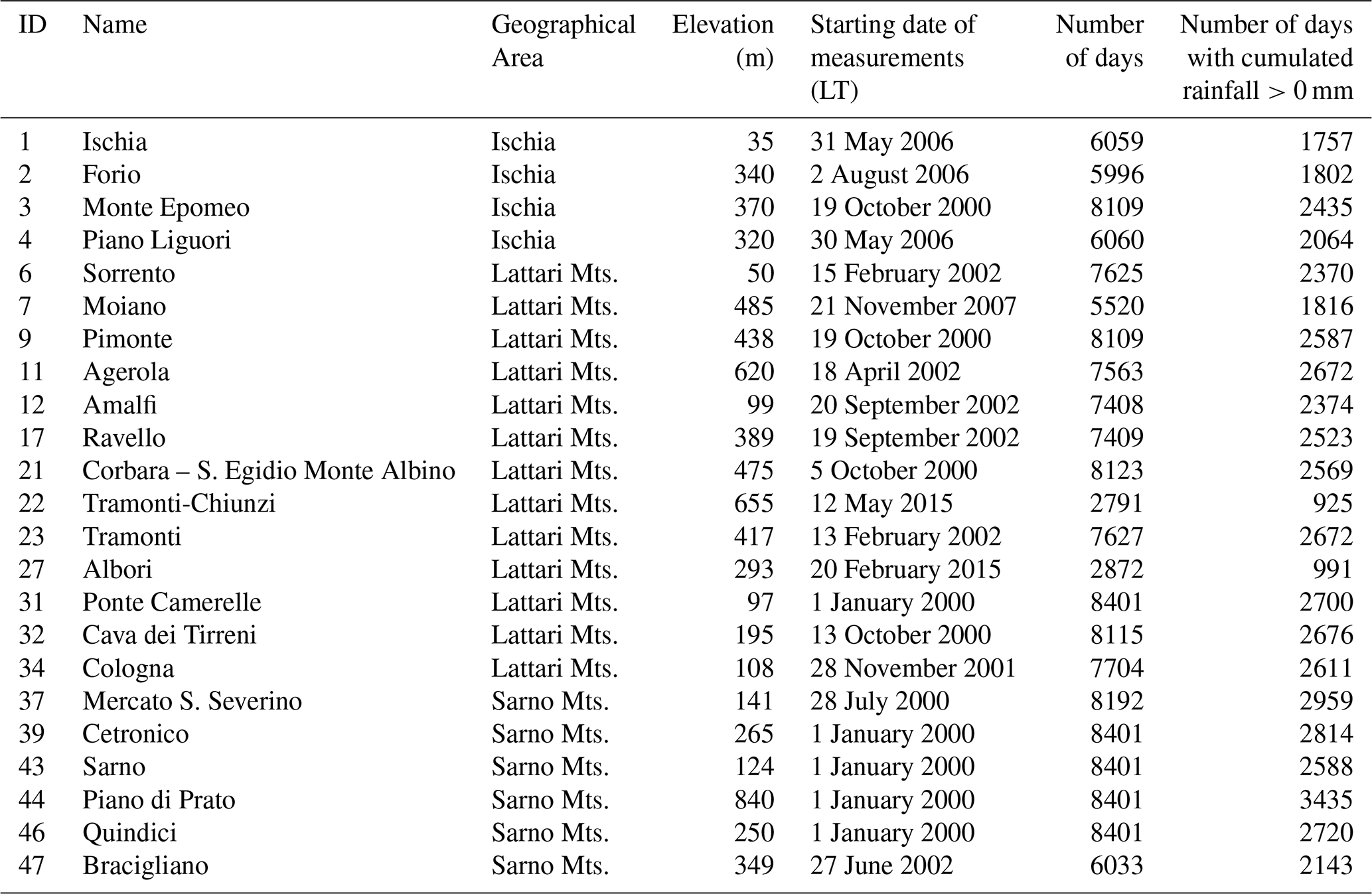
The rain gauges are located at elevations ranging from 35 to 840 m, with 52 % of them between 200 and 500 m. Distance between the rain gauges ranges from 1.7 to 11.8 km, with a mean of 5.9 km. The daily rainfall records cover different periods ranging from 2791 d (∼8 years, #22 Tramonti-Chiunzi, Lattari range) to 8401 d (∼22 years, #31 Ponte Camerelle, Lattari Mts), all ending on 31 December 2022 (Table 1). In the periods covered by each rain gauge record, the completeness of the measurements varies (Fig. 4). For two rain gauges (#1, Ischia Porto and #4, Piano Liguori, Table 1) the daily record is complete and, on average, for 0.4 % of the days in the records (31 d) no rainfall measurement is available (“no data”). For convenience, we assigned a value of 0.0 mm of rainfall to all the days in the records with missing rainfall information. This assumption may introduce a potential source of bias if missing observations occurred preferentially during intense or prolonged rainfall events, potentially leading to a slight underestimation of rainfall. However, the proportion of missing data is very limited (approx. 1.5 d each year, on average), and therefore the potential bias introduced by this assumption is expected to have a negligible impact on the overall analyses. On average, for 32.9 % of the days in the records the measured rainfall exceeded 0.0 mm (Table 1).

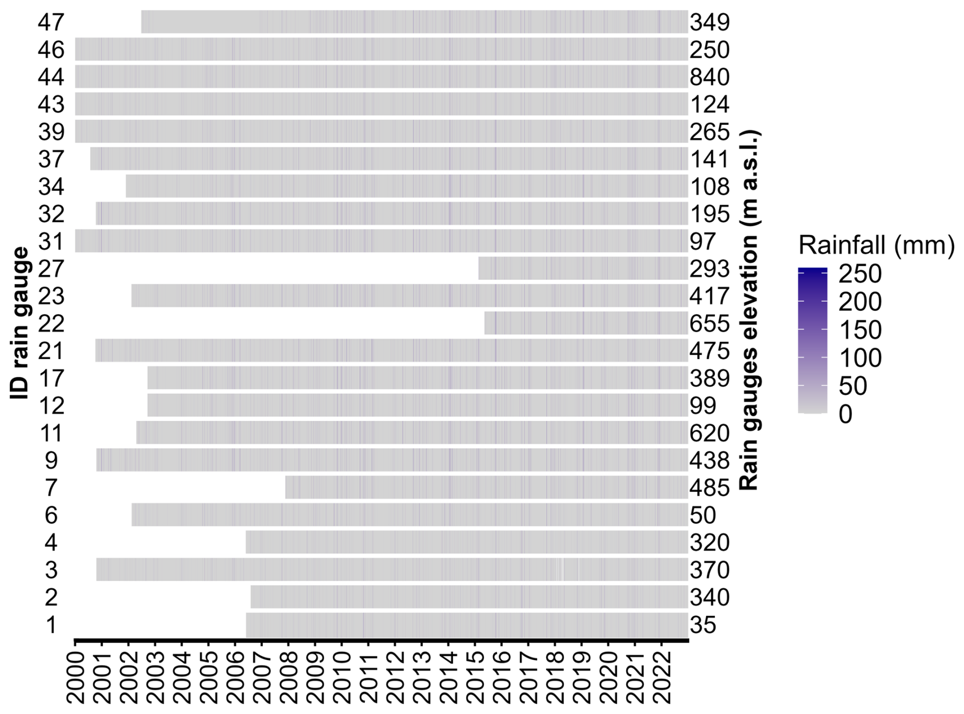
Figure 4 Rainfall time series recorded by the rain gauges in the study area. Each row corresponds to a rain gauge. Each vertical line represents a day in the rainfall record. Colour of each line show amount of daily rainfall.

3.3 Landslides – rainfall association

To investigate the rainfall conditions that led to landslides in the study area, we assign each landslide in the catalogue to the nearest rain gauge within a planimetric distance of 5 km. With this approach, we assume that the rainfall recorded at the rain gauge corresponds to the rainfall that fell in, or in the vicinity of the landslide and that triggered the landslide.

Using this selection criterion, we removed one landslide, and we associate 86 landslides (50.9 %) with a rain gauge within 2 km (Fig. 5).

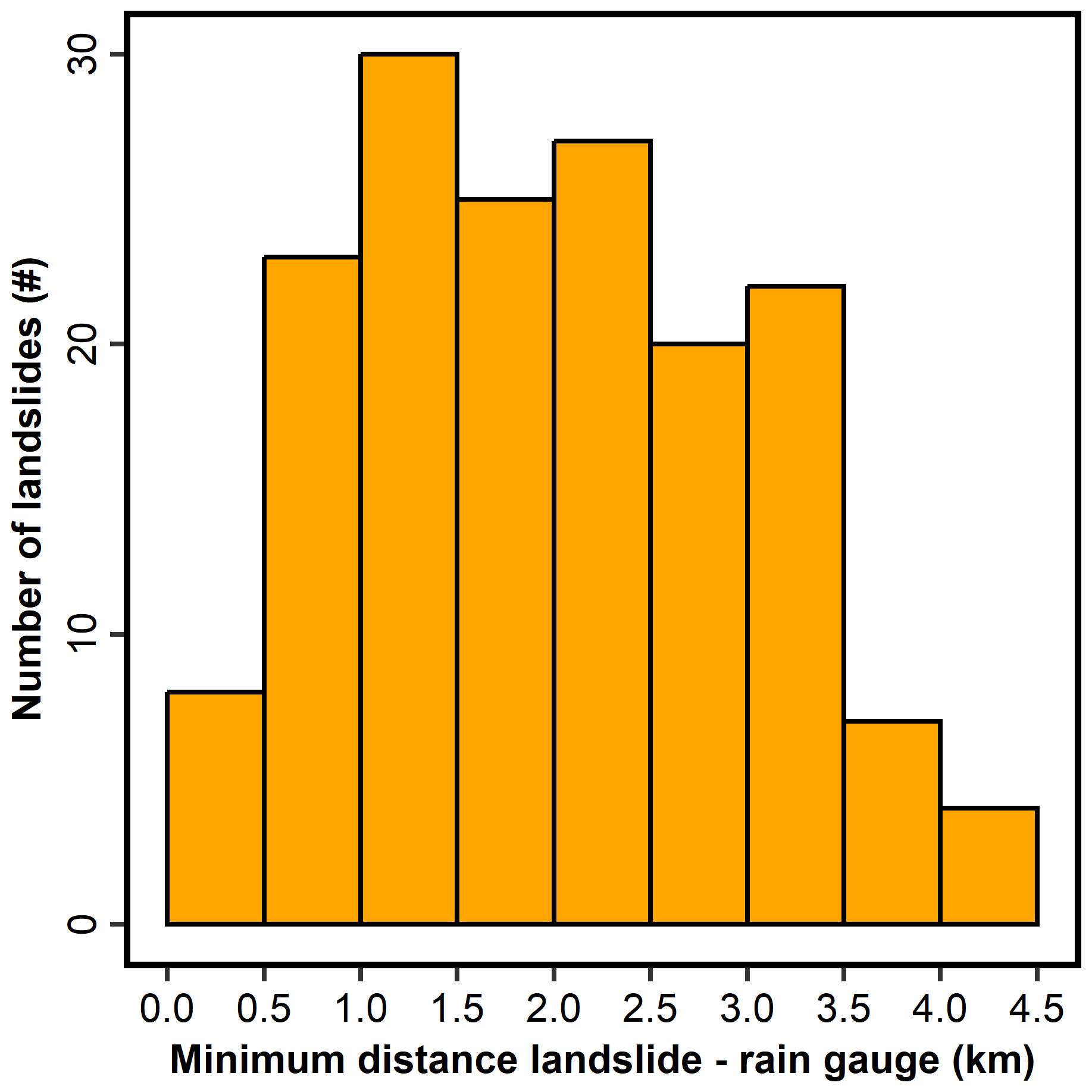
Figure 5 Distribution of the minimum distance between the landslide identification points and the rain gauges.

Overall, each rain gauge is associated with between 1 and 23 landslides, with an average of 7 landslides per gauge (Fig. 6). Since the day of the landslide is known, we assign to each day in the rainfall record of each rain gauge the total number of landslides that occurred on that day (from 0 (none) to 9 landslides) to obtain, for each rain gauge, a record that includes the date, amount of daily rainfall, and number of landslides. We use these records to calculate the landslide occurrence probability which we associate to the corresponding rain gauge.

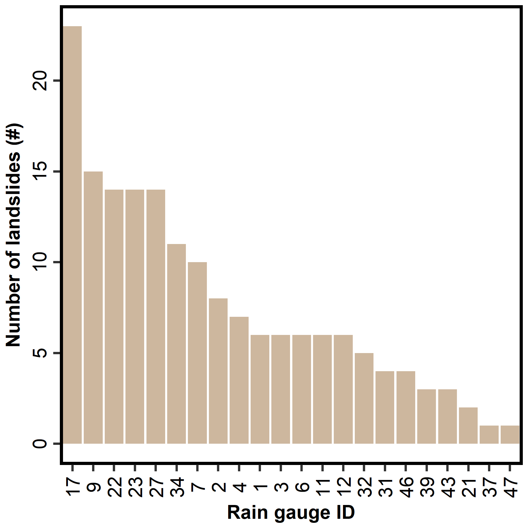
Figure 6 Number of landslides associated with each rain gauge. See Fig. 1 for location of landslides and rain gauges.

To determine the geographical area of influence of each rain gauge, in a GIS we construct Thiessen polygons (Thiessen and Alter, 1911) (Fig. 1). Within each polygon, with areas ranging between 8 and 94 km², average 37 km², there are between 0 (none) and 22 landslides. The landslide counts within each polygon are not the same as the number of landslides associated to the corresponding rain gauge based of the minimum distance between the landslide and the rain gauge. However, we choose to use the Thiessen polygons to associate the probability of occurrence of the landslide, calculated for each rain gauge, to the area of influence of each rain gauge.

4 Methods

4.1 Probabilistic framework

Here, we describe a general probabilistic framework for Bayesian landslide forecasting. The approach allows to incorporate all known uncertainties. We consider the binomial random variable L, where ℓ=0 if no landslides occur in the investigated space-time domain Ω, and ℓ=1 otherwise. We further consider Ω to be composed of a space domain A, and a forecasting time window ${\mathit{\tau }}_{\mathrm{0}}=[t_{\mathrm{0}},t_{\mathrm{0}}+\mathrm{\Delta }t]$, where t₀ is the beginning of a forecasting time window of length Δt. We separate the landslide occurrence $\stackrel{\mathrm{̃}}{\mathrm{\ell }}$ in τ₀ from the past landslide occurrence ℓ in the past forecasting time windows τ_j<t₀. For a generic landslide trigger y, the probability of landslide occurrence in τ₀ is given by

$$\begin{array}{}\text{(1)}& \text{Pr}(\stackrel{\mathrm{̃}}{\mathrm{\ell }}=\mathrm{1})={\int }_{\mathrm{0}}^{\mathrm{\infty }}p\left(\stackrel{\mathrm{̃}}{y}\right)\cdot \text{Pr}(\stackrel{\mathrm{̃}}{\mathrm{\ell }}=\mathrm{1}|\stackrel{\mathrm{̃}}{y})\mathrm{d}\stackrel{\mathrm{̃}}{y}\end{array}$$

where, $p\left(\stackrel{\mathrm{̃}}{y}\right)$ is the probability density function (PDF) i.e., the forecast of the trigger $\stackrel{\mathrm{̃}}{y}$, in the forecasting time interval τ₀, and $\text{Pr}(\stackrel{\mathrm{̃}}{\mathrm{\ell }}=\mathrm{1}|\stackrel{\mathrm{̃}}{y})$ is the conditional probability mass function of landslide occurrence for τ₀, given the trigger $\stackrel{\mathrm{̃}}{y}$. Adopting uniformitarianism (Lyell, 1830; Varnes and the IAEG Commission on Landslides and other Mass-Movements, 1984; Hutchinson, 1995), we assume that the landslide triggering process was the same in the past as it will be in the future i.e., that landslides will occur in the future under the same triggering conditions that led to landslides in the past. Hence, $\text{Pr}(\stackrel{\mathrm{̃}}{\mathrm{\ell }}=\mathrm{1}|\stackrel{\mathrm{̃}}{y})\equiv \text{Pr}(\mathrm{\ell }=\mathrm{1}\left|y\right)$, where the latter is associated to any generic forecasting time window τ_j<t₀. Using the Bayes theorem (Gelman et al., 2014), we may relate the past probability of landslide occurrence $\text{Pr}(\mathrm{\ell }=\mathrm{1}|y)$, in the forecasting time window τ₀, to the probability of landslide occurrence in the same forecasting time window τ₀, without information on the trigger,

$$\begin{array}{}\text{(2)}& \text{Pr}(\mathrm{\ell }=\mathrm{1}|y)={\displaystyle \frac{\text{Pr}(\mathrm{\ell }=\mathrm{1})\cdot p\left(y\right|\mathrm{\ell }=\mathrm{1})}{p\left(y\right)}}\end{array}$$

where, Pr(ℓ=1) is the probability mass function of landslide occurrence in the forecasting time interval τ₀ (the prior probability), $p\left(y\right|\mathrm{\ell }=\mathrm{1})$ is the conditional PDF of the trigger y, given landslide occurrence ℓ (the likelihood), and p(y) is the PDF of the trigger, in a generic forecasting time window τ_j. Note that p(y) and $p\left(\stackrel{\mathrm{̃}}{y}\right)$ are different. The former is the PDF of the trigger recorded in a generic forecasting time window (τ_j), whereas the latter is the PDF of the trigger in the future (τ₀) i.e., the landslide forecast of interest to us.

4.2 Application to rainfall-triggered landslides

We apply the general probabilistic framework described above to rainfall-triggered landslides in our study area (Fig. 1). For the purpose, we assume that rainfall is the sole trigger of landslides in the area, and we take a rainfall measurement that is obtained from the available rainfall record to describe the landslide trigger. In particular, we use the cumulative daily rainfall E, and we set seven rainfall thresholds y_t=0.2, 5, 10, 20, 30, 50, and 70 mm for each day to explore the possible existence of thresholds in the rainfall conditions that may result in landslides. Hence, we consider the binomial random variable $R\equiv Y>y_{\mathrm{t}}$, i.e., r=1 if the (cumulative) rain exceeds a selected threshold y_t, 0 otherwise.

Given the geographical and temporal resolution of the landslide and the rainfall data, we make the landslide forecasts at the location of the rain gauges, and we assume that the spatial domain of the forecast, coincides with the Thiessen polygon constructed around each rain gauge. In other words, we calculate the landslide occurrence probability at the location of the rain gauge by using the daily rainfall-landslide record, and we associate the calculated probability to the area of influence of the rain gauge. We further take Δt=1 d as the forecasting time window, and we obtain the probabilities necessary to solve Eq. (2) (the Bayes theorem) from the landslide catalogue and the available daily rainfall records at each rain gauge.

For each subregion, we rewrite Eq. (2) as,

$$\begin{array}{}\text{(3)}& \text{Pr}(\mathrm{\ell }=\mathrm{1}|Y>y_{\mathrm{t}})={\displaystyle \frac{\text{Pr}(\mathrm{\ell }=\mathrm{1})\cdot \text{Pr}(Y>y_{\mathrm{t}}|\mathrm{\ell }=\mathrm{1})}{\text{Pr}(Y>y_{\mathrm{t}})}}\end{array}$$

Therefore, assuming that the rainfall exceeds the threshold, the equation becomes,

$$\begin{array}{}\text{(4)}& \text{Pr}(\mathrm{\ell }=\mathrm{1}|r)={\displaystyle \frac{\text{Pr}(\mathrm{\ell }=\mathrm{1})\cdot \text{Pr}\left(r\right|\mathrm{\ell }=\mathrm{1})}{\text{Pr}\left(r\right)}}\end{array}$$

where, $\text{Pr}(\mathrm{\ell }=\mathrm{1}|r)$ is the posterior probability of landslide occurrence given a rainfall exceedance in τ₀, Pr(ℓ=1) is the prior probability of landslide occurrence in τ₀, $\text{Pr}\left(r\right|\mathrm{\ell }=\mathrm{1})$ is the probability of a rainfall exceeding the threshold given a forecasting time window τ_j, with at least one landslide, and Pr(r) is the exceedance probability of a selected rainfall threshold.

For the real example at hand, we obtain the prior, daily probability of landslide occurrence Pr(ℓ=1), from the landslide record of the corresponding rain gauge as the number of days with landslides in the record, d_L divided by the total number of days in the record, d

$$\begin{array}{}\text{(5)}& \text{Pr}(\mathrm{\ell }=\mathrm{1})={\displaystyle \frac{d_L}{d}}.\end{array}$$

Owing to the pervasive underreporting of landslides in the catalogue, the prior probability given by Eq. (4) provides a minimum boundary of the true, unknown value.

We obtain the likelihood, $\text{Pr}\left(r\right|\mathrm{\ell }=\mathrm{1})$ from the rainfall and landslide record as the ratio of the number of days with daily rainfall exceeding the threshold and having at least one landslide occurrence, d_R,L and the number of days with at least one landslide, d_L

$$\begin{array}{}\text{(6)}& \text{Pr}\left(r\right|\mathrm{\ell }=\mathrm{1})={\displaystyle \frac{d_{R,L}}{d_L}}.\end{array}$$

Use of Eq. (6) implies an important assumption: that landslides are effectively triggered by the exceedance of the daily rainfall threshold. This assumption will be indirectly checked during the analysis because, if it is incorrect, we should not expect any significant information coming from the occurrence of rainfall.

We obtain the exceedance probability of a given rainfall threshold Pr(r), as the ratio of the number of days with exceeding rainfall threshold, d_R, and the number of days in the record d,

$$\begin{array}{}\text{(7)}& \text{Pr}\left(r\right)={\displaystyle \frac{d_R}{d}}.\end{array}$$

Then, applying Bayes theorem (Eq. 4), we obtain the sought posterior probability of landslide occurrence given an exceedance rainfall of a specific threshold for each rain gauge in the study area. The procedure described above, applied using R software (R Core Team, 2025), is summarized and schematically illustrated in Fig. 7a.

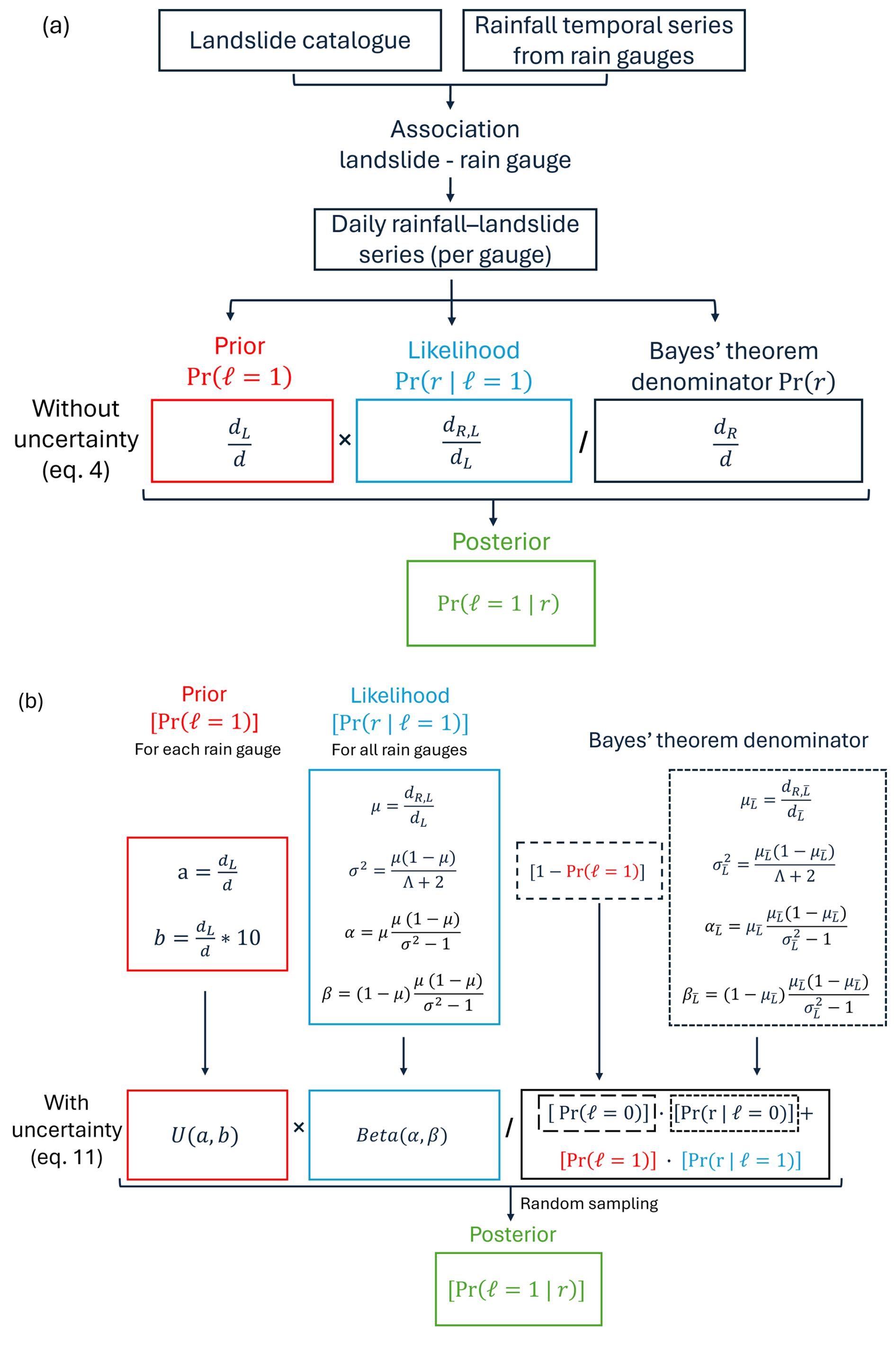
Figure 7 Workflow of the application of the Bayesian probabilistic procedure. (a) Application of Bayes' theorem without uncertainty. (b) Application of Bayes' theorem accounting for uncertainty. See Appendix B for mathematical symbols.

4.3 Modelling spatial and temporal resolution

The aim of our model is to provide the probability of landslide occurrence given a rainfall exceeding r, $\text{Pr}(\mathrm{\ell }=\mathrm{1}|r)$, in a one-day time window within the area of influence of the rain gauge i.e., the corresponding Thiessen polygon (Fig. 1). The temporal resolution of the probability of landslide occurrence is defined (imposed) by the daily resolution of the rainfall data. Further, the time of the landslide occurrence is known only for part of the record (see Sect. 3.1). Even when the time is known, it still brings an uncertainty because it is usually inferred and not directly measured. For this reason, we attribute each landslide only to the known or inferred day of occurrence. As said before for Eq. (6), the consequence of this time resolution is that we ought to assume that the cumulative daily rainfall is responsible for the landslide triggering, whereas a landslide may be triggered by the rainfall fallen in part of a day.

The spatial resolution of the model depends on the spatial resolution of the landslides and the rain gauges. Whereas the accuracy in geographical location of the rain gauges is high (meters to tens of meters), the location of the landslides is affected by uncertainty ranging from tens to several hundreds of metres, or even larger for landslides whose geographical coordinates were located in the deposit or at the landslide toe, i.e. distant from the (unknown) failure initiation point. To address the problem, we attribute the probability of landslide occurrence $\text{Pr}(\mathrm{\ell }=\mathrm{1}|r)$, to the rain gauge used to calculate it. Then, we associate this probability is to the corresponding Thiessen polygon (Fig. 1) assuming that the rainfall conditions around the rain gauge are homogeneous within the area of influence of the rain gauge.

4.4 Modelling of uncertainties

Like many natural hazards, landslide occurrence is characterized by uncertainties of different kind. Uncertainties are related to the intrinsic complexity (e.g., nonlinearly coupled variables) of the landslide occurrence process that does not allow for a deterministic prediction, to the incompleteness of the landslide information (see Sect. 3.1), and to the accuracy and completeness of the rainfall record (see Sect. 3.2). Additional uncertainty arises from the association of the landslides and the rainfall records (see Sect. 3.3) depending on the daily resolution of the rainfall information, and the different (and possibly distant) locations of the rain gauges and the landslides. Albeit of difficult quantification, these uncertainties affect the estimates of the probability of landslide occurrence.

The inclusion of uncertainties requires the adoption of a probabilistic framework in which a probability is not a single value, but a distribution. Intuitively, the distribution of probability describes how much we are sure about the probability estimated. Formally, the problem is more convoluted, and it requires a clear definition of what probability means and why a distribution of probability makes sense (Marzocchi and Jordan, 2014; Marzocchi, 2018). Here, we just say that a probability is a frequency of landslides in a well-defined “experimental concept”. The distribution of probability describes where the true unknown frequency is expected to be.

To model the uncertainty related to the incompleteness of the catalogue, we use a uniform distribution as a prior (Fig. 8a). This non-informative prior is the simplest way to represent a state of ignorance about the value of a parameter – in this case, the true and unknown frequency of landslide occurrence. By using a uniform distribution, we assume that each value of the landslide frequency has an equal probability of being sampled. The lower limit of the distribution corresponds to the prior calculated by using Eq. (5), i.e., the landslide frequency obtained by the catalogue. We set the upper limit one order of magnitude higher than the lower limit, assuming that we were able to record one landslide for every ten that occurred in reality, consistently with the well-documented incompleteness of landslide catalogues (Guzzetti, 2002; Peruccacci et al., 2023). We used this approach to obtain a prior uniform distribution for each rain gauge.

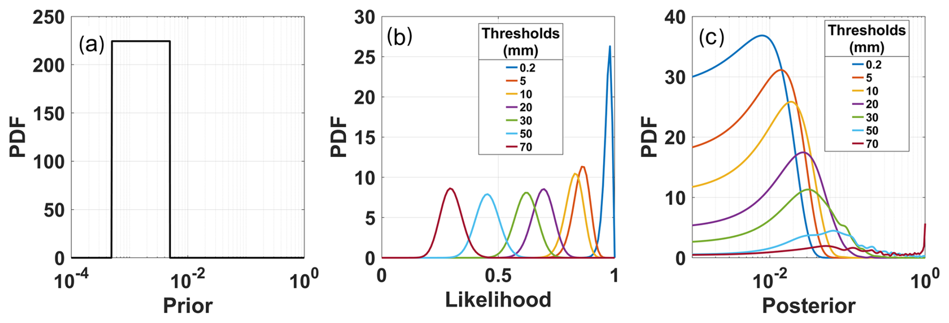
Figure 8 Probability distributions. (a) Uniform prior probability for rain gauge #1 in Table 1. (b) Beta likelihood distributions corresponding to seven different rainfall thresholds; the same distributions are applied to all rain gauges. (c) Posterior distribution of rain gauge #1, obtained by multiplying the uniform prior (a) by each of the likelihood distributions (b).

The distribution of the likelihood incorporates multiple sources of uncertainty, including those related to the landslide information and the rainfall measurements, as the likelihood represents the probability of rainy days (days with recorded rainfall) when landslides were reported. We model this probability using a beta distribution, Beta(α,β), which is particularly suitable for describing a parameter that ranges between zero and one (Gelman et al., 2014). The spread of the Beta distribution (Fig. 8b) therefore conveys the uncertainty arising from incomplete landslide catalogues and potential measurement errors in rainfall data. Other distributions defined over the same domain can be used, yielding similar results, as the specific choice of distribution is not a critical factor (Gelman et al., 2014). The parameters α and β were calculated by using the following equations:

$$\begin{array}{}\text{(8)}& {\displaystyle }\mathit{\alpha }=\mathit{\mu }\cdot {\displaystyle \frac{\mathit{\mu }(\mathrm{1}-\mathit{\mu })}{{\mathit{\sigma }}^{\mathrm{2}}-\mathrm{1}}}\text{(9)}& {\displaystyle }\mathit{\beta }=(\mathrm{1}-\mathit{\mu })\cdot {\displaystyle \frac{\mathit{\mu }(\mathrm{1}-\mathit{\mu })}{{\mathit{\sigma }}^{\mathrm{2}}-\mathrm{1}}}\end{array}$$

where, μ is calculated using Eq. (6) applied to the rainy days with reported landslides for all rain gauges and for each rainfall threshold. In other words, we consider all days with landslides and the corresponding rainfall across all rain gauges to compute μ, which represents the likelihood in the case without uncertainty. σ² is the variance of the rainy days with landslides calculated as

$$\begin{array}{}\text{(10)}& {\mathit{\sigma }}^{\mathrm{2}}={\displaystyle \frac{\mathit{\mu }(\mathrm{1}-\mathit{\mu })}{\mathrm{\Lambda }+\mathrm{2}}}\end{array}$$

where, Λ is the equivalent number of data, related to the sample size used to define the beta distribution. We use Λ=98, corresponding to the total number of rainy days with at least one reported landslide across all rain gauges.

Assuming that the physical processes of landslide triggering in the study area are the same (indeed, the catalogue lists landslides of the similar type, i.e., shallow flow-like landslides), we use all the rainy days with landslides for each rain gauge. Thus, we combine the data from all rain gauges, obtaining a single distribution of the likelihood for all the gauges, and we obtain different likelihood distributions for each rainfall threshold (Fig. 8b). Note that the distributions of prior and likelihood are calculated over different time periods. This is because in the case of likelihood, we combine the days of all the rain gauges, covering the 20-year catalogue. Conversely, we define the prior distribution for the individual rain gauges which cover different time periods (see Sect. 3.2). Implicitly, we are assuming that the characteristics of the rainfall triggering rainfall events did not change over the 20-year period of time covered by the landslide catalogue.

We obtain the posterior probability distribution through the Bayes theorem,

$$\begin{array}{}\text{(11)}& \begin{array}{rl}& \left[\text{Pr}\right(\mathrm{\ell }=\mathrm{1}\left|r\right)]=\\ & {\displaystyle \frac{\left[\text{Pr}\right(\mathrm{\ell }=\mathrm{1}\left)\right]\cdot \left[\text{Pr}\right(r|\mathrm{\ell }=\mathrm{1})]}{\left[\text{Pr}\right(\mathrm{\ell }=\mathrm{1}\left)\right]\cdot \left[\text{Pr}\right(r|\mathrm{\ell }=\mathrm{1})]+[\text{Pr}(\mathrm{\ell }=\mathrm{0})]\cdot [\text{Pr}\left(r\right|\mathrm{\ell }=\mathrm{0}\left)\right]}}\end{array}\end{array}$$

where, the square brackets indicate the use of a distribution of the argument, $\text{Pr}(\mathrm{\ell }=\mathrm{0})=\mathrm{1}-\text{Pr}(\mathrm{\ell }=\mathrm{1})$, and $\text{Pr}\left(r\right|\mathrm{\ell }=\mathrm{0})$ is calculated as in Eq. (6) considering rainy days with no landslides ($d_{R,\stackrel{\mathrm{‾}}{L}}$). The posterior distribution is obtained by sampling randomly [Pr(ℓ=1)], $\left[\text{Pr}\right(r|\mathrm{\ell }=\mathrm{1})]$, and $\left[\text{Pr}\right(r|\mathrm{\ell }=\mathrm{0})]$. Assuming that the uncertainties of the three distributions are independent, we sample the distributions independently. The distribution of the posterior probability is obtained numerically through the application of the Bayes' theorem for each set of randomly sampled values. In this way, for each rain gauge we obtain seven posterior probability distributions, for the seven selected rainfall thresholds. An example of the posterior probability distributions is shown in Fig. 8c for the Ischia rain gauge (# 1 in Fig. 1), in the Ischia Island. Figure 7b schematically summarizes the procedure described above, applied by using MATLAB^® software (The MathWorks Inc., 2024).

4.5 Evaluating forecast improvement with the probability gain

To investigate whether, and to what extent, the information on rainfall (i.e., the application of Bayes' theorem given by Eq. 4) has improved our landslide forecast, we calculate the “probability gain”, the ratio between the posterior and the prior probability, for each rain gauge (Kass and Raftery, 1995). Since the prior probability contains only landslide information (Eq. 5), whereas the posteriori probability contains both landslide and rainfall information (Eq. 4), the probability gain weights the rainfall information on the landslide forecast to quantify the improvement (“gain”) in the forecasting skill using the additional rainfall information. The larger the probability gain, the larger the weight of the rainfall information on the forecast. If the probability gain is 1, the information given by the rainfall is negligible, because the posterior and the prior probability equals. With probability gain increasing, the rainfall information becomes more important to improve the skill of the forecast. We calculate the probability gain for each rain gauge by considering both the probabilities without uncertainty and the probabilistic distributions. In the latter case, we compute the gain as the ratio of the posterior median value to the prior median value.

4.6 Model validation

Within the proposed probabilistic framework, model validation can be performed in a prospective way as new landslide events are added to the inventory, by comparing predicted posterior probabilities with future observed occurrences. A classical train/test split validation would not be suitable for this approach, as the landslide inventory is limited. Random data partitioning would significantly reduce the number of landslide occurrences available for the probabilistic calculations, leading to statistically weak and potentially misleading results, and affecting the posterior estimates rather than providing a robust assessment of predictive skill. It is important to emphasize that the aim of this study is not to develop a purely predictive classifier specific to a given area, but rather to provide a mathematical framework to optimally use all available information and quantify probabilistic relationships between rainfall conditions (or any other triggering mechanism) and landslide occurrence. However, in this work, considering the current lack of independent data, model results are checked for logical and physical consistency, verifying that posterior probabilities increase with increasing cumulative daily rainfall. To further assess the robustness of the posterior estimates, future work may explore the sensitivity of the results to different prior and likelihood formulations.

5 Results

5.1 Application to rainfall triggered landslides in the study area

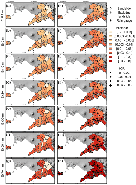
The maps in Figs. 9–11 show the probability in each Thiessen polygon i.e., in each area of influence of each rain gauge in the study area (Fig. 1), considering and not considering uncertainty.

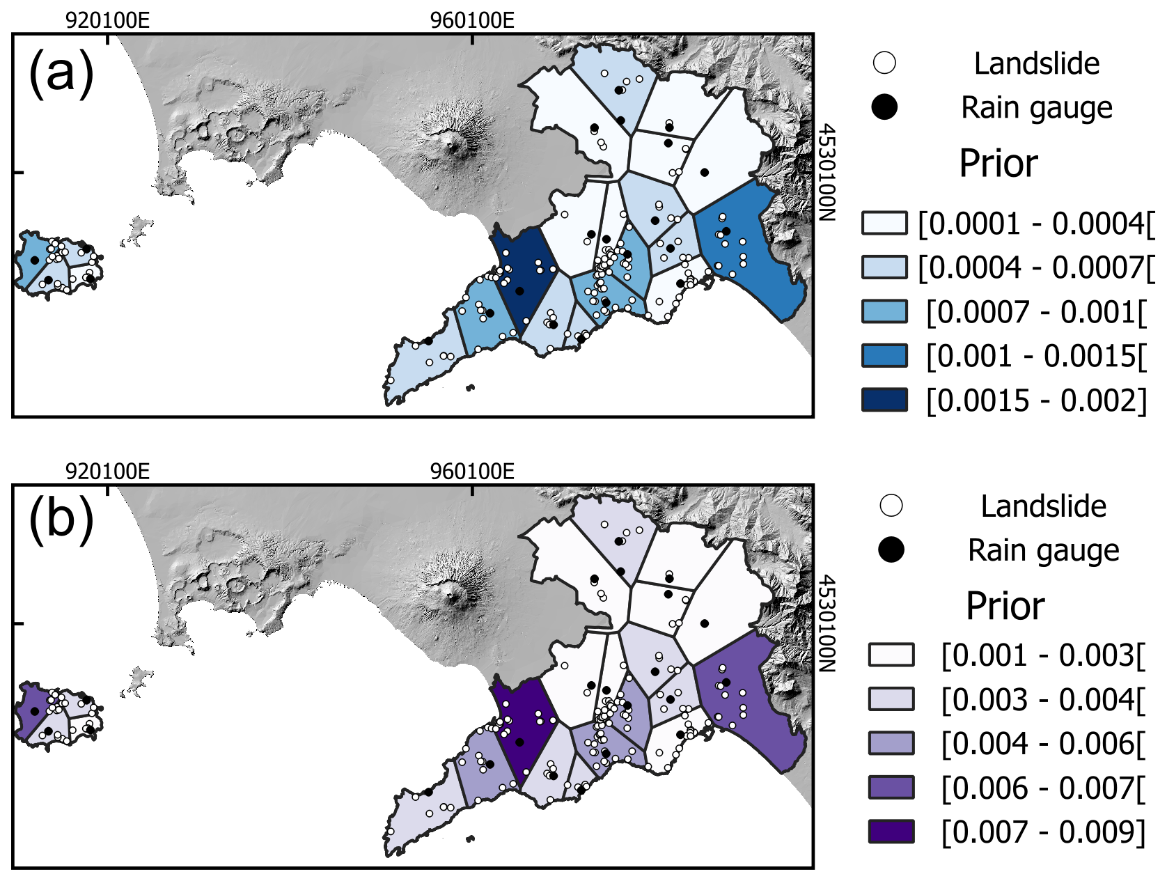
Figure 9 Maps of prior probability. (a) Non considering uncertainty. Prior probabilities calculated for each rain gauge using Eq. (5). (b) Considering uncertainty. Median posterior probabilities obtained using Eq. (11).

Figure 10 Maps of likelihood probability for different rainfall thresholds. (a) Not considering uncertainty. Likelihood probabilities obtained for each rain gauge by applying Eq. (6). (b) Considering uncertainty. Likelihood probabilities obtained for each rain gauge using the median of the distributions derived from Eqs. (8) and (9).

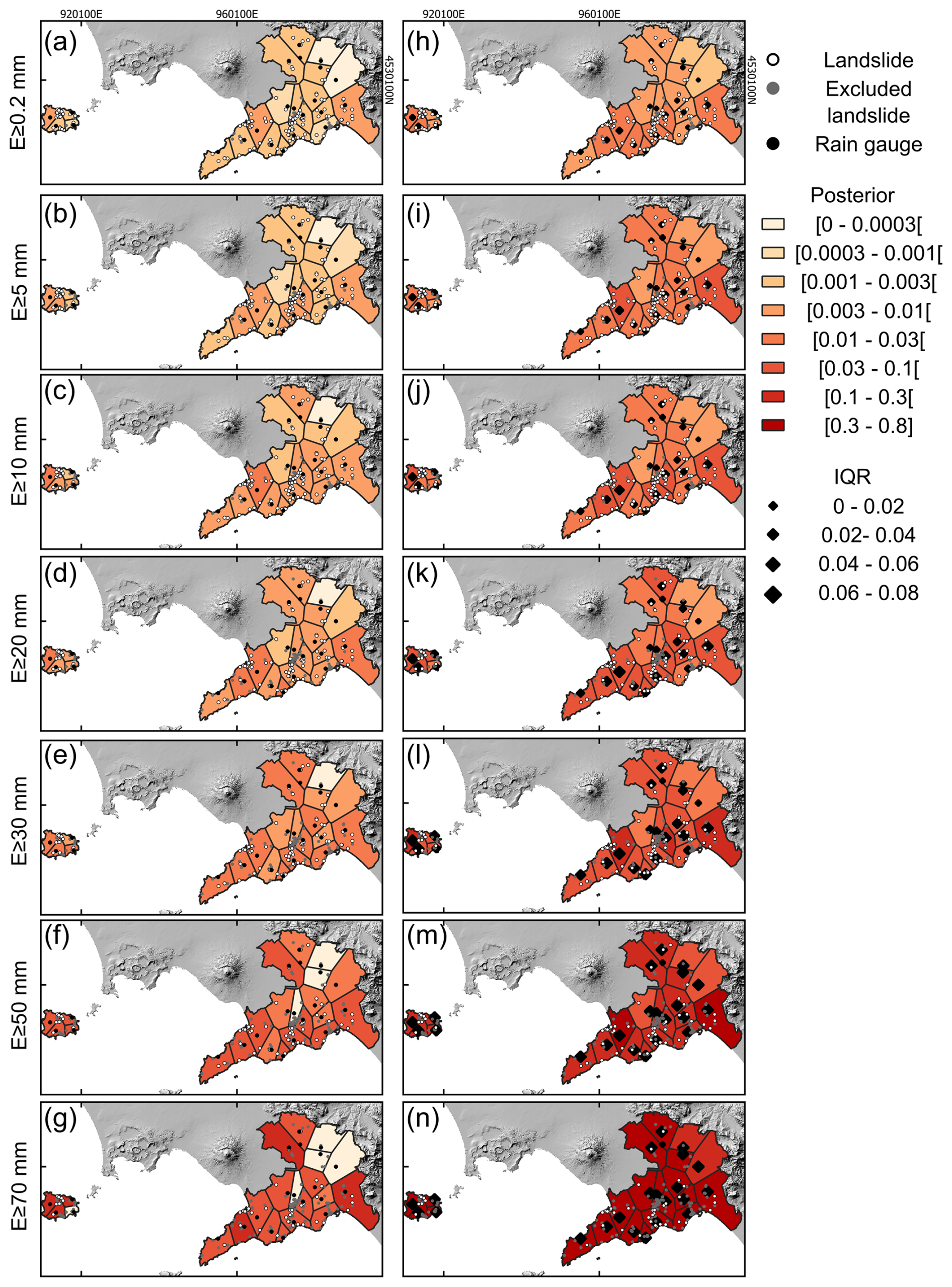
Figure 11 Maps of posterior probability for different rainfall thresholds. (a) Posterior probabilities not considering uncertainty obtained using Eq. (4). (b) Median posterior probabilities considering uncertainty obtained using Eq. (11).

Figure 9 illustrates the geographical distribution of the prior probability. In Fig. 9a, when uncertainty is not considered (Eq. 5), the prior probabilities are in the range 10⁻⁴ to 10⁻³, depending on the number of days with landslides linked to each rain gauge. On average, each rain gauge has seven days with landslides. If some of the landslides associated to a rain gauge occurred in the same day, the number of days with landslides further decreases. On average, four days with landslides are recorded per rain gauge, whose rainfall record spans approximately 6000 d (about 16.6 years). Consequently, the ratio $\mathrm{4}/\mathrm{6000}$ yields a probability of approximately 10⁻⁴. This explains why probabilities of around 10⁻⁴ are the most frequently observed. In Fig. 9b, when uncertainty is considered (as shown in the example of Fig. 8b), the prior probabilities are higher, in the range 10⁻³–10⁻². The increase reflects the effect of under-reporting in the landslide catalogue. Joint inspection of Fig. 9a and b shows that the Thiessen polygon (rain gauge) associated with the highest prior probabilities, considering and not considering uncertainty, is the same (#9, Pimonte), as expected.

Figure 10 illustrates the geographical distribution of the likelihood associated with each of the seven rainfall thresholds, both not considering (Fig. 10a–g) and considering (Fig. 10h–n) uncertainty. In both cases, the likelihood ranges between 0 and 1, due to how we calculate likelihood (see Sect. 4.2). When uncertainty is not considered (Eq. 6), likelihood values are equal to 1 when the number of rainy days with landslides matches the total number of days with landslides. This implies that, on each day with reported landslides, the recorded rainfall exceeded the corresponding threshold. On the contrary, when days with landslides are associated with rainfall amounts below the threshold, the likelihood is less than one, because the number of rainy days with landslides is less than the total number of days with landslides that remains constant – being independent of rainfall (Eq. 6). These landslides occurring on days with rainfall below the threshold are not accounted for in the likelihood estimation, and they are represented as grey dots in Fig. 10. When uncertainty is accounted for, the likelihood is modelled as a Beta distribution defined on the interval [0,1] (Eqs. 8–10).

In Fig. 10a–g, for the lowest rainfall threshold (0.2 mm), the likelihood is equal to 1 for most rain gauges, as all associated landslides occurred on days with daily rainfall E>0 mm. An exception is rain gauge #47 (Bracigliano, in the Sarno mountain range) for which the likelihood is zero, as it is linked to a single landslide that occurred on 26 December 2004, a day when no rainfall was recorded by the Bracigliano rain gauge. As the rainfall threshold increases, the likelihood decreases. Similar observations apply when uncertainty is considered (Fig. 10h–n), bearing in mind that for each threshold we use a single likelihood distribution for all rain gauges (Fig. 8b). In this case, we assigned the median value of the distribution corresponding to each rainfall threshold to the respective Thiessen polygon. For low thresholds (0.2, 5, and 10 mm), the median likelihood ranges between 0.8 to 1. As the threshold increases, the median likelihood decreases, as higher thresholds exclude days when landslides occurred under lower rainfall conditions. This trend is illustrated in Fig. 8b, where increasing the rainfall thresholds (i.e., moving from right to left in the plot) causes the distribution peak to shift towards lower values. Additionally, the distributions become more dispersed, reflecting increased variance in the data.

By applying Eqs. (4) and (11) to all rain gauges, we obtain the posterior probability $\text{Pr}(\mathrm{\ell }=\mathrm{1}|r)$ and $\left[\text{Pr}\right(\mathrm{\ell }=\mathrm{1}\left|r\right)]$ of at least one day with landslides in each Thiessen polygon and for each rainfall threshold. The resulting posterior probability maps are shown in Fig. 11. For clarity, the posterior probabilities are represented on a logarithmic scale in both sets of maps. When uncertainty is not considered (Fig. 11a–g), the posterior probabilities for the lowest rainfall threshold (0.2 mm) range between 0 and 10⁻³. As the rainfall threshold increases, the posterior probabilities also increase, reaching up to 10⁻¹ for the highest threshold (70 mm). However, for the 50 and the 70 mm thresholds, some Thiessen polygons show a decrease to zero of the posterior probability. This occurs when landslides associated with the rain gauge took place on days with rainfall below the threshold. When considering uncertainty (Fig. 11h–n) the median posterior probabilities follow a similar pattern, increasing with higher rainfall thresholds. Probabilities range from 10⁻³ to 10⁻² for the lowest threshold (0.2 mm), and from 0.2 to 0.8 for the highest threshold (70 mm). In Fig. 11h–n, the Thiessen polygons (rain gauges) do not exhibit the apparently inconsistent decrease in probability at the highest thresholds that is observed in Fig. 11a–g. This highlights the importance of incorporating uncertainty into the analysis, as this produces a more consistent pattern that compensates for the limitations in the available data.

Overall, the posterior probability accounting for uncertainty is, on average, higher than that computed without uncertainty, for all thresholds. We attribute the result to the fact that the observed landslide frequency is set to the minimum value of the prior distribution, to account for under-reporting in the landslide catalogue. As a result, the median value of the prior distribution is greater than the observed frequency, which in turn leads to a higher median value of the posterior distribution. Moreover, as the rainfall threshold increases, the posterior distribution that incorporates uncertainty becomes progressively wider. To assess this dispersion, we calculate the interquartile range (IQR), defined as the difference between the third and first quartiles of the posterior distributions. The IQR values are shown in Fig. 11h–n by the size of the black diamonds, which grow larger with higher rainfall thresholds, indicating broader distributions. The pattern is also illustrated in Fig. 8c, which shows an example for the #1 Ischia rain gauge.

5.2 Probability gain

Figure 12 summarizes the probability gains calculated for each rain gauge and rainfall threshold. Green points represent the probability gains obtained by dividing the prior by the posterior probabilities calculated with Eqs. (4) and (5), without accounting for uncertainty. Blue dots are calculated using the median values of the prior and the posterior probability distributions, and error bars are obtained by dividing the 5th and 95th percentile of the prior and posterior distributions. In both cases – whether uncertainty is considered or not – the probability gain increases almost linearly with the rainfall threshold. For any given threshold, the probability gains calculated without considering uncertainty exhibit a wider variability.

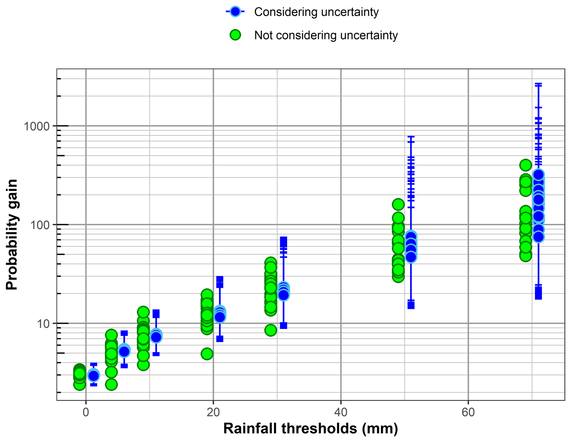
Figure 12 Probability gains for each rain gauge as a function of the rainfall thresholds. Green dots represent probability gains calculated not considering uncertainty. Blue dots represent the median of the probability gains. Error bars show the 5th and 95th percentiles of the probability gain distribution for each rain gauge. Green and blue dots refer to the same rainfall threshold value and are horizontally offset for visualization purposes.

To better visualize the number of rain gauges associated with specific probability gains for each rainfall threshold, Fig. 13 shows the cumulative distributions of the probability gains. The curves, one of each threshold, show the percentage proportion of rain gauges (y axis) with a probability gain equal or less than the corresponding value on the x axis. For example, in Fig. 13a – not considering uncertainty – for the rainfall threshold E≥20 mm, approximately 20 % of the rain gauges have a probability gain of 10 or less, implying that 80 % of gauges have a probability gain greater than 10. In contrast, when considering uncertainty (Fig. 13b), all rain gauges exhibit probability gains close to 10. Overall, the results indicate that increasing the rainfall threshold leads to a larger portion of the study area experiencing an improvement in the forecast skill, due to the inclusion of rainfall information.

Figure 13 Probability gain cumulative curves. y axis shows percentage of rain gauges associated with the corresponding x axis value of the probability gain. (a) Values calculated not considering uncertainty. (b) Median values calculated considering uncertainty.

6 Discussion

We have proposed and applied a Bayesian framework to forecast the possible occurrence of landslides. The probabilistic approach accounts for the epistemic uncertainty in landslide forecasting which arises from incomplete knowledge of the boundary conditions (e.g. slope conditions, values of governing factors) in addition to uncertainties in the available data. A key feature of the proposed framework is the use of probability distributions, enabling the explicit inclusion and representation of all sources of uncertainty, while keeping them distinct. By relying on distributions instead of single-point estimates, we can systematically describe our current state of knowledge regarding both the landslide process and data.

In the example application we have presented, the shape of the posterior distribution (representing the probability of landslide occurrence given the exceedance of a specified rain threshold) varies across different thresholds, illustrating how uncertainty propagates through the forecasting process. Notably, the variance of the posterior distribution increases with higher rainfall thresholds, reflecting the accumulation of epistemic uncertainty in both the prior probability and the likelihood. The spread of the posterior distribution measures the level of confidence in the “true” (and unknown) probability: the broader the distribution, the wider the plausible range for the true probability (assuming the model is correct), and thus, the lower our confidence in pinpointing the exact probability value. Importantly, the posterior probability that incorporates uncertainty is more informative than the corresponding probability computed not considering the uncertainty. It provides a more realistic representation of the uncertainties associated with our understanding of the factors controlling slope instability, the limitations of the available landslide catalogue, and the inherent randomness of the landslide initiation. Within this probabilistic framework, model validation can be performed in a prospective way as new landslide events are added to the catalogue, by comparing predicted posterior probabilities with future observed occurrences. To further assess the robustness of the posterior estimates, additional future developments may investigate the sensitivity of the results to different prior and likelihood formulations.

Applying the method to a real-world case allowed us to explore how the probability gain varies with rainfall thresholds, offering further insight into the mechanisms of rain-induced landslide occurrence. Firstly, the fact that probability gain is consistently greater than one underscores the importance of incorporating rainfall information to enhance landslide forecasting. Secondly, if landslide triggering were governed by a well-defined physical threshold, this would be reflected in the behaviour of the probability gain. Specifically, we would expect a step-like change at a critical threshold value. However, as shown in Fig. 12, the observed trend is gradual and approximately linear. The finding challenges the notion of a sharp, physical rainfall threshold for landslide occurrence, and instead supports the view that the probability of landslide occurrence increases progressively with the accumulation of rainfall. The gradual trend also reduces the dependence of the results on the specific set of thresholds adopted in the analysis.

These findings have important implications for the potential operational use of the proposed methodology (Piciullo et al., 2018; Guzzetti et al., 2020). The absence of sharp, physical thresholds suggests that any threshold adopted for practical landslide risk reduction actions must be selected on a careful evaluation of costs and benefits (Staley et al., 2013); for example, thresholds ought to be selected balancing the rates of false alarms and missed events.

A strength of the proposed probabilistic framework lies in its potential for generalization. Since the approach models the evolution of landslide occurrence probability as a function of the probability of a generic triggering process, the term y in Eq. (2) could equally represent, for example, the ground shaking caused by an earthquake. The only requirement is the availability of a time series of historical records of the chosen trigger alongside a corresponding record of landslide occurrences. Therefore, the posterior probability can be obtained either without accounting for uncertainty (by using the frequencies of days with landslides triggered by a specific type of ground shaking) or by incorporating uncertainty using probabilistic distributions. Once the probability of landslide occurrence has been estimated (regardless of the trigger) it can be compared with the probability of occurrence of other natural hazards (e.g., earthquakes, tsunami, volcanic eruptions) occurring within the same spatio-temporal window. The probabilities of occurrences can be obtained from conceptual models which, like our proposed framework, are based on historical records of triggering events (Marzocchi et al., 2008).

The proposed probabilistic framework can also be applied to different or larger regions and extended time periods, assuming that sufficient information is available. In our application, geological information is accounted for by focusing on a geologically homogeneous area and by using a catalogue comprising similar types of shallow rainfall-induced landslides. For short-term forecasting, rainfall data is typically sufficient to model the potential occurrence of future landslides, even in large and complex landscapes (Mondini et al., 2023). As the forecast window increases, the influence of transient rainfall inputs diminishes, and environmental factors become more dominant. Consequently, geological information should be explicitly incorporated into the model.

When considering a longer temporal window, the meteorological conditions assumed to be constant may vary, particularly in the context of climate change. By adopting the principle of uniformitarianism (Lyell, 1830; Varnes and the IAEG Commission on Landslides and other Mass-Movements, 1984; Hutchinson, 1995), we assume that the physical processes responsible for landslide triggering remain unchanged over time. This implies that, although climate change may alter the frequency and intensity of rainfall events (thereby affecting the rate of landslide occurrence) the underlying physical triggering mechanisms remain unchanged. Within this framework, climate change influences the probability distribution of future rainfall events, and not the landslide triggering process itself, which remains stationary.

The proposed framework has limitations, the main of which is the availability and quality of input data (Berti et al., 2012; Guzzetti et al., 2025). Uncertainties related to the completeness and reliability of both the landslide and the rainfall records propagate through the probabilistic results. For this reason, the framework would greatly benefit from a large volume of high-quality data; in their absence, uncertainty can become the dominant factor. Our model illustrates the point.

Within this context, the use of daily rainfall data represents an additional limitation of the present application of the framework. The choice was primarily dictated by the temporal accuracy of the available landslide catalogue, which predominantly reports event occurrence at the daily scale and often relies on inferred rather than directly observed timing of landslide occurrence (Peruccacci et al., 2023), and by the availability of rainfall data at daily temporal resolution. Adopting rainfall data at finer temporal resolutions would therefore not be consistent with the resolution of the landslide records and could introduce further uncertainty. At the same time, the daily scale reflects the temporal resolution at which operational warning assessments are commonly issued by the Campania Regional Authority, supporting the practical applicability of the framework. Although antecedent rainfall conditions are known to influence shallow landslide occurrence in pyroclastic soils (Napolitano et al., 2016), daily rainfall can still provide meaningful predictive information because many landslides are associated with short-duration intense rainfall events occurring during the wet season (Rianna et al., 2014), when antecedent conditions are often already close to critical levels. In this sense, part of the effect of antecedent wetness conditions may already be implicitly embedded in the empirical rainfall-landslide relationship captured by the dataset, since many landslides of the catalogue occurred in autumn and winter (see Fig. 3a). Future research could explore the influence of different rainfall accumulation periods to assess whether, and to what extent, antecedent conditions affect landslide occurrence. This could be investigated by cumulating antecedent rainfall over progressively longer periods (e.g., 1, 2, 7, 15 d).

A further limitation concerns the spatial association between rainfall measurements and landslide occurrence. In the present study, Thiessen polygons are adopted to define the area of influence of each rain gauge, consistently with approaches commonly used in operational early warning systems, including the Campania regional warning system for hydrogeological hazards (D. P. G. R. n. 299 30/06/2005, 2005). Although this method provides a pragmatic and computationally efficient spatial partitioning, it represents a geometric approximation that does not explicitly account for topographic and orographic controls on rainfall variability. Alternative approaches based on hydrological catchments, or topographically informed interpolation methods could potentially provide a more physically based representation of rainfall forcing. However, the available spatial density and distribution of landslides and rain gauges limited the applicability of more detailed spatial subdivisions, which frequently resulted in spatial units containing insufficient data for the probabilistic analysis.

Related to the spatial assumptions discussed above, the construction of a single likelihood distribution from all rain gauges combined implicitly assumes stationarity and spatial homogeneity of the rainfall-landslide relationship across the study area. This is a simplifying assumption, partly motivated by the limited size of the available landslide catalogue. Indeed, pooling data across rain gauges increases the sample size and reduces the uncertainty in the likelihood estimates, at the cost of smoothing out local variability. Stationarity implies that the statistical relationship between rainfall and landslide occurrence is assumed constant over the observation period, an assumption that could be violated if climate change progressively alters the frequency and intensity of extreme rainfall events, or if land use changes. However, the assumption is considered reasonable over the 22-year observation period and within the geologically homogeneous setting of the study area. The assumption of homogeneity is broadly consistent with the geological and geomorphological setting of the study area, which includes similar shallow landslide types triggered by short-duration, high-intensity rainfall events. However, the validity of these assumptions is indirectly supported by the results themselves: the consistent increase in probability gain with rainfall threshold across all rain gauges would not emerge if the assumed likelihood structure were fundamentally inconsistent with the data. A spatially heterogeneous or non-stationary relationship would tend to introduce noise and suppress the trend observed in Fig. 12. Nevertheless, we recognize that these assumptions represent a limitation of the current implementation. Future developments incorporating gauge-specific likelihood distributions, longer records, or higher-resolution rainfall data would allow these assumptions to be explicitly tested, potentially improving both the accuracy and the spatial resolution of the posterior probability estimates.

In addition to data-related limitations, the proposed framework is inherently constrained by its exclusive reliance on historical rainfall and landslide records. As a result, it cannot provide an operational “next day” landslide forecast when no rainfall measurements are available. This would require the integration of quantitative rainfall forecasts from meteorological modelling. This limitation reflects the operational logic of the regional landslide early warning system adopted by the Campania Regional Authority, which is primarily based on thresholds of observed cumulative rainfall, rather than on meteorological forecasts (Calvello et al., 2016). The integration of rainfall forecasts into the proposed probabilistic structure (see Eq. 1) is conceptually straightforward and represents a promising direction for future research. However, this would also introduce additional challenges (notably, the differences between the spatial and temporal scales of weather forecasts (Strandberg and Lind, 2021) and those used in the model) that would need to be carefully addressed.

7 Conclusions and perspectives

We developed and applied a Bayesian probabilistic framework to forecast landslides, explicitly accounting for the sources of epistemic uncertainty affecting landslide occurrence. By relying on probability distributions rather than single-point estimates, our modelling framework integrates incomplete and uncertain information from both landslide and rainfall records, offering a realistic and flexible approach to landslides forecasting. The application of the framework to shallow landslides in parts of the Campania region, Southern Italy (Fig. 1), demonstrated its capability to produce spatially and temporally resolved estimates of landslide occurrence probability. The results reveal a progressive increase in posterior probability with increasing rainfall thresholds, ranging from 0 to 10⁻³ at the lowest threshold (0.2 mm) to up to 10⁻¹ at the highest threshold (70 mm) when uncertainty is not considered, and from 10⁻³ to values between 0.2 and 0.8 at the highest threshold (70 mm) when uncertainty is accounted for, without evidence of a sharp, physical threshold. This finding supports the interpretation of landslide triggering as a probabilistic rather than deterministic process and highlights the importance of using probability gain to quantify forecast improvement.

Our results have potential direct implications for operational early warning systems. While thresholds are useful for decision-making, their definition is inherently uncertain and can introduce substantial arbitrariness. We show in this paper that they lack specific scientific meaning. Conversely, a probabilistic framework enables thresholds to be set via explicit cost–benefit trade-offs that reflect operational priorities (Piciullo et al., 2017). In a probabilistic cost–benefit approach, thresholds are set to balance false alarms against missed events by considering both expected losses and expected costs of mitigation actions. As Fischhoff et al. (1981) note in their treatise on acceptable risk, a risk is acceptable only if it is compensated by corresponding benefits.

Further, the general structure of the proposed framework makes it adaptable to other triggers, such as earthquakes, provided appropriate data are available. Indeed, a limitation of the approach is the availability and quality of the input data. Improvements in landslide catalogues and rainfall records, especially with higher spatial and temporal resolution, would significantly enhance the model's performance. Future research could explore the influence of antecedent rainfall and alternative accumulation periods and expand the model's application to broader spatial scales or different geomorphological settings.

Appendix A

Table A1 Information listed in the landslide catalogue used in the study.

Appendix B: Mathematical symbols and acronyms

P	Probability
L	Binomial random variable of landslide occurrence
ℓ	Past landslide occurrence
$\stackrel{\mathrm{̃}}{\mathrm{\ell }}$	Future landslide occurrence
Ω	Space-time domain of the forecast
τ0	Time domain of the forecast, ${\mathit{\tau }}_{\mathrm{0}}=t_{\mathrm{0}}+\mathrm{\Delta }t$
τj	Past time domain, ${\mathit{\tau }}_{\mathrm{0}}=t_j<t_{\mathrm{0}}$
t0	Beginning of the forecasting time domain
tj	Time before the beginning of the forecasting time domain
Δt	Length of the time domain
y	Generic landslide trigger
R	Binomial random variable of triggering rainfall
d	Days in the record
dL	Days with landslides in the record
dR	Days with rainfall in the record
dR,L	Days with rainfall and landslides in the record
$d_{R,\stackrel{\mathrm{‾}}{L}}$	Days with rainfall and no landslides in the record
U(a,b)	Uniform distribution between the lower (a) and upper (b) limit
Beta(α,β)	Beta distribution, with parameters α and β
PDF	Probability distribution function
PMF	Probability mass function
E	Cumulative daily rainfall threshold