Developing a coastal hazard prediction system in ice-infested waters – Part 1: High-resolution regional wave modeling in the Estuary and Gulf of St. Lawrence

This study is the first of a two-part paper that summarizes the development of a prototype coastal hazard prediction system providing short-term (+48 h) forecasts of the total water level (TWL) at 50 m resolution for the province of Quebec, Eastern Canada. In this first part, the implementation of the offshore wave model component of the system, which is a regional 1 km-resolution WAVEWATCH III™ (WW3) configuration for the Estuary and Gulf of St. Lawrence (EGSL), is presented and discussed. The configuration is forced by high resolution atmosphere, ocean and sea ice forecasts provided by Environment and Climate Change Canada (ECCC) and includes a state-of-the-art parameterization of wave propagation and attenuation in sea ice that has been tuned with observations from the EGSL. Performances are assessed against wave data collected over a 2-year period during which the forecasting system was running operationally, and against historical storm data using a model hindcast. Results demonstrate reasonable forecast skills both for normal and extreme wave conditions during ice-free periods with errors ranging from 15 % to 31 % of the mean wave height. However, when sea ice is present, performances are drastically reduced, primarily due to inaccuracies in the predicted ice fields at spatial scales over which wave energy typically dissipates in sea ice.

1 Introduction

The Canadian coastline surrounding the Estuary and Gulf of St. Lawrence (EGSL) is frequently impacted by coastal hazards such as storm-induced coastal flooding (Didier et al., 2019), due to overwash and overtopping, inflicting severe damages to coastal communities and nearshore infrastructures (Friesinger and Bernatchez, 2010; Didier et al., 2015; Bernatchez et al., 2011). Storms also cause sudden and significant geomorphological changes including nearshore profile adjustments, beach, dune, and cliff erosion and barrier breaching in Atlantic Canada (Forbes et al., 2004). The last two extreme events to date, the post-tropical storms Dorian in September 2019 and Fiona in September 2022 caused considerable damages to docks, roads and private properties. The cumulative insured losses were estimated at over USD 105 million (IBC, 2020) and USD 800 million (IBC, 2023) respectively, with a large proportion being caused by water-related damages. There are currently more than 700 000 people in Atlantic Canada living within 1 km of the coastline, of which 88 000 reside less than 5 m above mean sea level (MSL) (Statistics Canada, 2024). The projected costs due to the damage to coastal infrastructure by the retreat of the coast, if no adaptation measures are implemented, are estimated at USD 1.5 billion only for the Eastern Quebec on the 2065 horizon (Bernatchez et al., 2015). Enhancing community preparedness to such hazards is crucial to mitigate their impact and ensure public safety. Coastal risk management involves implementing appropriate Disaster Risk Reduction (DRR) measures that include efficient short-term forecasting tools to support decision-making and emergency response.

Coastal flooding events occur when the total water level (TWL) at the coast rises abnormally high through the combination of the astronomical tide (η_T), the nontidal residuals (η_NT) and wave-induced effects (η_W).

$$\begin{array}{}\text{(1)}& \text{TWL}={\mathit{\eta }}_{\mathrm{MSL}}+{\mathit{\eta }}_{\mathrm{T}}+{\mathit{\eta }}_{\mathrm{NT}}+{\mathit{\eta }}_{\mathrm{W}}\end{array}$$

where η_MSL is the mean sea level relative to some vertical datum. The nontidal residuals (η_NT) includes fluctuations of the water level associated with storm surges generated by atmospheric pressure anomalies (inverted barometer effect) and wind stress acting on the sea surface (wind setup), as well as low-frequency seasonal water level variations, including land ice melt, ocean circulation or river discharge. The wave contribution to TWL (η_W), includes the wave set-up – a superelevation resulting from the wave radiation stress induced by breaking waves – and the wave run-up which is the sum of the wave set-up and the maximum swash uprush. Run-up and swash can be partitioned into the incident wave band and the infragravity component (Stockdon et al., 2006; Didier et al., 2020), which may be generated due to the presence of short-wave groups (bound infragravity waves) or locally in response to fluctuations in radiation stress induced by the fact that longer waves break further from the coast than smaller ones.

The relative contribution of η_T, η_NT and η_W to TWL can vary significantly depending on the type of environment (Serafin et al., 2017; Li et al., 2022). Nonetheless, analyses of historical coastal flooding events consistently highlight the prominent role of wave-induced processes (Didier et al., 2015) that in certain cases dominate the TWL signal (Hoeke et al., 2013; Leijnse et al., 2025) and should therefore receive particular attention. While TWL is typically represented as a linear superimposition of processes (Eq. 1), there are numerous interactions between them (Idier et al., 2019). For example the fact that the mean water level influences wave dissipation and therefore the transfer of momentum to the nearshore water column. This makes the problem highly nonlinear and complicates both the physical interpretation and prediction of coastal flooding events.

The EGSL is a semi-enclosed sea open to the Atlantic through the Cabot and Belle-Isle Straits. In addition to medium to short fetch distances, the region is partially covered with sea ice during winter. A significant part of this seasonal ice cover is composed of rather thin unconsolidated ice adjacent to open water (Galbraith et al., 2024), similar to what is found in the marginal ice zone (MIZ) that marks the transition between open water and the inner ice pack in polar regions.

By reducing the fetch, sea ice prevents extreme sea states to develop during the winter storm period. Landfast ice (sometimes referred to as nearshore ice) also provides temporary shore protection by acting as a natural breakwater, which reduces potential storm impacts at the coast (Forbes et al., 2002, 2004; Manson et al., 2016). However, the ongoing reduction of the seasonal sea ice cover in the EGSL is likely to intensify the wave climate and increase the frequency of occurrence of extreme wave events (Ruest et al., 2016; Wang et al., 2018) leading to flooding events and coastal erosion (Orviku et al., 2003; Ryabchuk et al., 2011). There are therefore raising concerns about the vulnerability of coastal populations in the context of climate change in cold regions.

In the last decade, considerable efforts have been made worldwide towards enhancing the predictability of coastal hazards with the aim of integrating it into Early Warning Systems (EWS). The MICORE program (Ciavola et al., 2011a, b), followed by the RISC-KIT project (Van Dongeren et al., 2018), were pioneering initiatives in developing fully integrated frameworks that combine coastal hazard forecasting and tools to support decision-making and risk management. One approach to coastal hazard prediction uses a cascade of numerical models from global and regional-scale (e.g. for tide, storm surge, and waves) down to beach-scale models such as Xbeach (Roelvink et al., 2009) and Delft3D (Lesser et al., 2004) aimed at resolving both storm-driven hydrodynamics and associated morphological changes. While these fully process-based numerical models have demonstrated excellent capabilities both for flood risk mapping (Gallien, 2016; Didier et al., 2019) and for representing morphodynamic response to storms (McCall et al., 2015), their high computational demands often restricts their use in the context of operational forecasting to a limited number of high-risk pilot sites, generally covering tens to hundreds of kilometers (Barnard et al., 2014). It therefore raises the question of their applicability at a national scale for countries that have thousands of kilometers of coastline. Some studies proposed tackling this issue by producing forecasts using probabilistic Bayesian Network (BN) trained by pre-run simulations of process-based models (Poelhekke et al., 2016; Garzon et al., 2023). Alternative methods also involve combining regional numerical models and semi-empirical wave run-up formulations to provide nowcasts and forecasts of TWL. This can be applied over larger areas due to lower computational constraints. The USGS (United States Geological Survey) Total Water Level and Coastal Change forecast system is an example of such a system (Aretxabaleta et al., 2019; Stockdon et al., 2023; Birchler et al., 2024). Regardless of their complexity, a common aspect of all approaches is that they all rely on numerical modelling to generate forcing wave conditions using third generation wave models such as WAVEWATCH III™ (Tolman, 2009) or SWAN (Booij et al., 1999). However, they have not been applied yet to ice-infested environments.

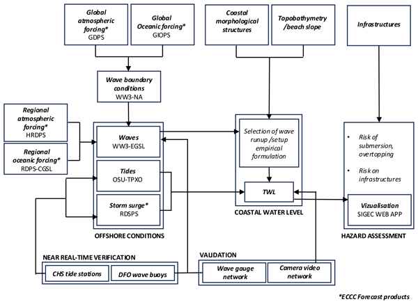
This two-part study introduces a newly developed deterministic coastal hazard forecasting system for the coasts of Québec, Canada. The system provides daily short-term (+48 h) TWL forecasts along 50 m spaced cross-shore transects. It integrates regional predictions of sea ice and water levels including tides and storm surge provided by Environment and Climate Change Canada (ECCC), along with a high-resolution 1 km third generation spectral wave model. The system follows a similar approach to that of (Stockdon et al., 2023) where wave run-up is estimated using semi-empirical equations based on offshore wave predictions and beach slopes derived from high-resolution LiDAR Digital Elevation Models (DEM). Coastal impacts and exposure are assessed using the classical Sallenger storm impact regimes (Sallenger, 2000). The overview of the system is shown in Fig. 1.

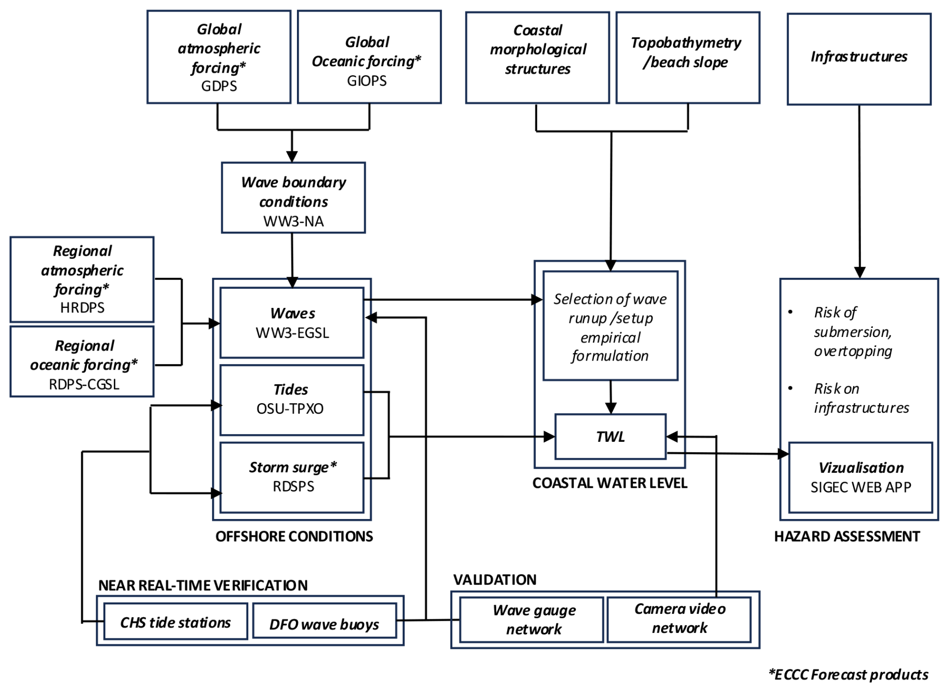
Figure 1 Schematic structure of the operational prediction system with its four main components: (i) an offshore module which merges wave, tide and storm surge predictions, coupled with (ii) a near real-time verification system for waves and water levels, (iii) a coastal water level modules that compute the TWL based on a set of calibrated empirical wave run-up/set-up equations, and (iv) a web-based visualization tool for coastal risk analyses.

This system was primarily designed to assess the risk of inundation, overwash, and overtopping, with a focus on evaluating the contribution of waves to the Total Water Level (TWL), which forms the core of this paper. Although geomorphological changes are important factors in assessing coastal risks, particularly on sandy coastlines, this aspect has been excluded from the study. The goal is to demonstrate the feasibility of providing reliable short-term TWL predictions at large scale in a seasonally ice-covered environment. The study aims to perform a comprehensive performance analysis of the system, identifying uncertainties, challenges, and limitations for its operational use within an Early Warning System (EWS).

The first part of this study focuses exclusively on the implementation and performance evaluation of the offshore wave component, with particular attention to the system's ability to predict extreme sea states. The discussion emphasizes the critical role of wind forcing selection and the challenges associated with wave-ice interactions. The detailed calculation of wave run-up, TWL, and coastal risk assessment are subjects of the second part of this study. The paper is structured as follows. Section 2 outlines the model configuration and implementation, Sect. 3 details the dataset used for evaluating forecast skills, Sect. 4 presents the performance assessment both in forecast and in hindcast modes during historical storm events and Sect. 5 discusses key challenges, lessons learned, and provides recommendations and future strategies to improve prediction accuracy.

2 Model Description

2.1 Configuration

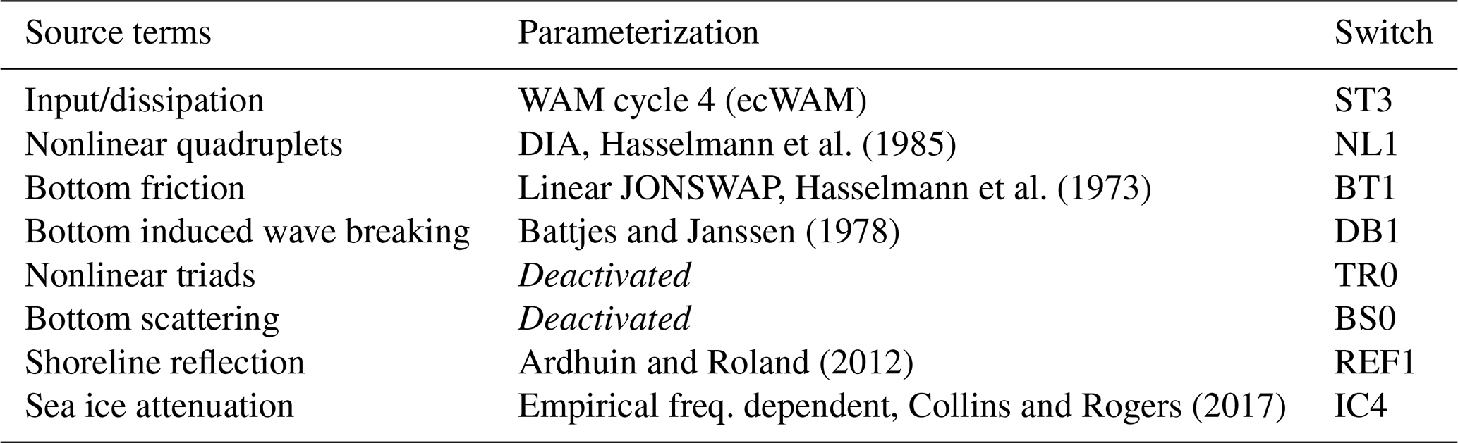
The wave forecasting system is based on a regional configuration of WAVEWATCH III™ v5.16 (WW3, Tolman, 2009) implemented on two domains. The first domain covers the Estuary and Gulf of St. Lawrence (EGSL) between 45.5 and 51.9° N latitude and 70 and 55° W longitude. The computational grid consists in a uniform rectilinear grid of 0.015 × 0.01° spatial resolution (∼ 1 km). The other domain covering the North Atlantic (NA) between 45.5 and 51.9° N latitude and 70 and 55° W longitude with 0.5° resolution is used to compute wave boundary conditions for the WW3-EGSL domain at Cabot Strait and Belle-Isle Strait (Fig. 2). The model bathymetry is obtained from the General Bathymetric Chart of the Oceans dataset (GEBCO v2019, GEBCO Bathymetric Compilation Group, 2019), developed through the Nippon Foundation-GEBCO Seabed 2030 Project which provides bathymetric data on a global coverage on a 15 arcsec grid. The wave spectrum is discretized into 25 frequency bins ranging from 0.05 to 0.5 Hz and 36 directions (10° resolution). Model parameters and source term specifications are listed in Table 1. One forecast cycle is initialized daily at 00:00 UTC and provides 48 h lead time predictions.

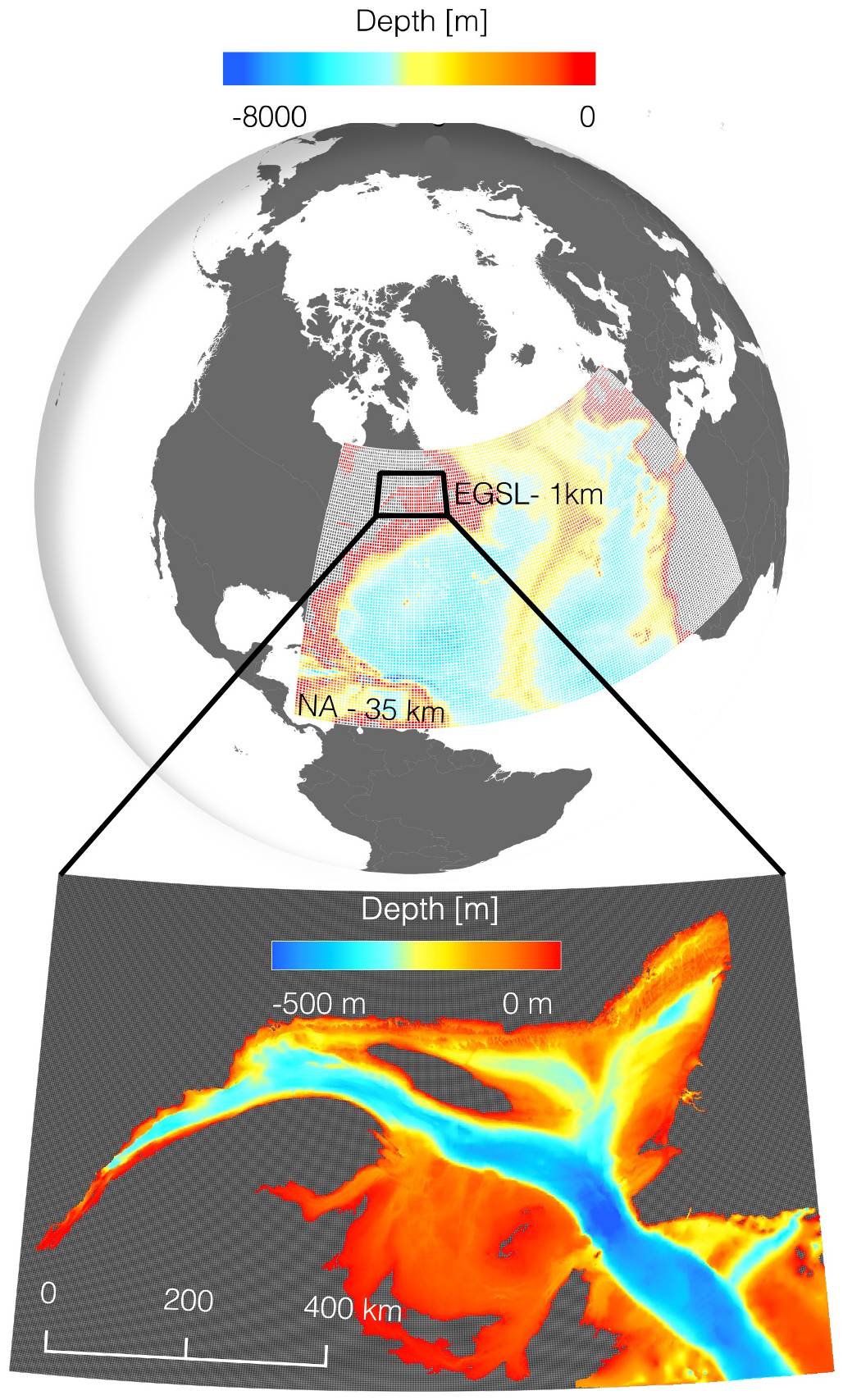
Figure 2 Digital grid and bathymetry of the North Atlantic (NA, top) and Estuary and Gulf of St. Lawrence (EGSL, bottom) configurations.

Hasselmann et al. (1985)Hasselmann et al. (1973)Battjes and Janssen (1978)Ardhuin and Roland (2012)Collins and Rogers (2017)

Table 1 Source terms and corresponding parameterizations used in the WW3 model configurations.

2.2 Forcing

2.2.1 Wind

The surface wind climatology in the EGSL exhibits a strong seasonal variability, characterized by dominant northwesterly winds averaging 4–7 m s⁻¹ in winter and weaker southwesterly winds ranging from 2–4 m s⁻¹ in summer (Perrie et al., 2015), with annual peaks reaching 15–20 m s⁻¹ (Hundecha et al., 2008). For such dominant winds, the fetch is significantly limited in some parts of the domain, particularly in the St. Lawrence Estuary (∼ 60 km at the widest). For 10 m winds, our configuration relies on two atmospheric forecast systems – one global and one regional – developed and maintained by the Meteorological Service of Canada (MSC). The Global Deterministic Prediction System (GDPS) is a coupled atmosphere-ocean-sea ice operational weather forecasting system. The atmospheric component is based on the Canadian Global Multiscale model (GEM) (Côté et al., 1998a, b) and the data assimilation system on a four-dimensional ensemble-variational (4DEnVar) approach (Buehner et al., 2013). It provides 3-hourly forecasts with 10 d lead time on a global 15 km-resolution grid with 28 vertical levels. The system runs twice a day (00:00 and 12:00 UTC) but since only one forecast cycle per day is carried out in our system, we only use the forecast produced at 00:00. This product is used to generate 10 m wind forcing for the NA domain.

The High Resolution Deterministic Prediction System (HRDPS) is the product developed by the MSC for short-term weather prediction at high resolution (2.5 km) covering the Canadian national area. It is based on a limited-area (LAM) configuration of GEM. The HRDPS is driven by GDPS, which provides lateral and upper boundary conditions for the atmospheric fields and uses the Canadian Land Data Assimilation System (Carrera et al., 2015, CalDAS). Hourly data are available at a horizontal resolution of about 2.5 km up on 31 vertical levels. Predictions are performed up to four times a day, but again, we only keep the 00:00 forecast.

The use of such high-resolution atmospheric model gives the opportunity to simulate the wave climate in short-fetch areas with great precision. Indeed, in sheltered coastal environments, the resolution of the wind model becomes determinant due to sharp spatial gradients in drag coefficients between land and the ocean (Long et al., 2016), which greatly influences the wind speed at 10 m. In order to quantify the impact of the spatial resolution of the wind model on the wave prediction in the EGSL, a comparison was made between a configuration forced by the NCEP (National Centers for Environmental Prediction) Climate Forecast System Reanalysis (CFSR, Saha et al., 2010) which has a spatial resolution of 35 km and one forced by HRDPS. Both simulations were run in hindcast mode for the year 2017 and evaluated against wave buoy observations (refer to Sect. 3 for details on the buoy network) deployed in the Estuary.

The comparison with observations (Fig. 3) reveals a tendency to underestimate wave heights in the simulations forced by CFSR, with an average bias of 0.26 cm and a regression slope of 0.49. In contrast, simulations using HRDPS show a marked improvement, with a much smaller bias of −0.04 cm and a regression slope of 0.86. The spatial analysis of the bias between the HRDPS- and CFSR-forced simulations (Fig. 3) allows identifying areas that are particularly sensitive to the choice of the wind model and demonstrates that high-resolution wind forcing significantly improves model accuracy in narrow and coastal areas, particularly in the Estuary, Chaleur Bay, and the Northumberland Strait.

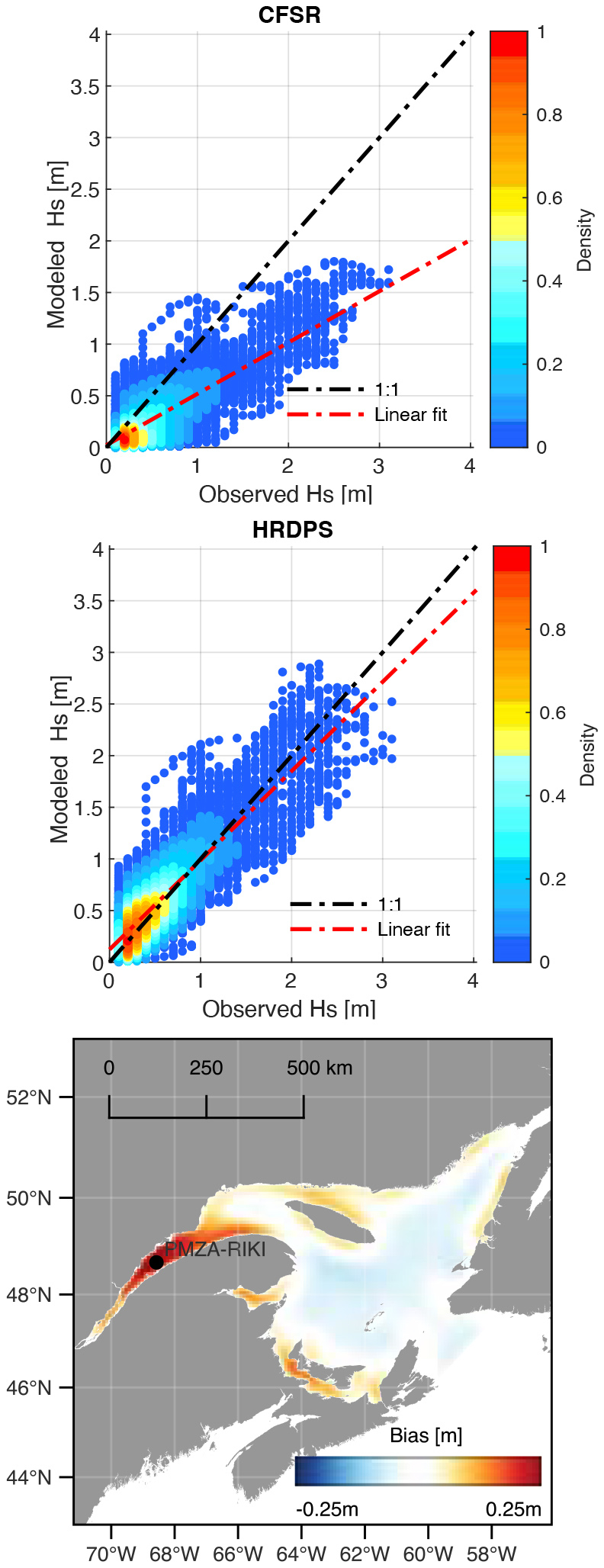
Figure 3 Comparison between observed and modelled significant wave height H_s at station PMZA-RIKI when forced by CFSR (top) and HRDPS winds (middle). The mean difference (HRDPS − CFSR) is shown in the bottom panel.

2.2.2 Ocean and sea ice

As with atmospheric forcing, the wave configuration uses surface currents and sea ice predictions provided by MSC from a global model for the NA domain and a regional model for the EGSL domain.

The Global Ice Ocean Prevision System (GIOPS) is an operational coupled ocean-sea ice forecasting and data assimilation system which is fully coupled with GDPS. The ocean component is based on the NEMO model (Nucleus for European Modelling of the Ocean) version 3.6 (Madec et al., 2017) and the sea ice component is based on CICE (Community Ice CodE) version 4.0 (Hunke and Dukowicz, 1997; Hunke et al., 2010). The data assimilation system is based on the System Assimilation Mercator Version 2 (SAM2) and combines satellite observations of sea level anomaly (SLA) and sea surface temperature (SST) as well as in situ observations of temperature and salinity (Smith et al., 2016). GIOPS runs once a day and provides 3h forecasts with 10 d lead time on a global $\mathrm{1}/\mathrm{4}$° resolution grid.

The regional model is the Coupled Atmosphere-Ice-Ocean Forecast System in the Gulf of St-Lawrence (RDPS-CGSL). It is a 5 km resolution configuration of NEMO-CICE which includes tides and freshwater inflows of rivers coupled to a limited area configuration (LAM) of the Regional Deterministic Prediction System (RDPS) centered over the EGSL. Satellite-derived observations of ice conditions from RADARSAT images are assimilated using a direct insertion method when available. The systems runs four times a day and provide hourly forecasts with 48 h lead time. Note that this system is no longer in use at MSC and has been supplanted by the new Coastal Ice and Ocean Prediction System (CIOPS).

2.3 Wave-ice interactions

The Gulf of St. Lawrence is a seasonally ice-covered semi-enclosed sea connecting the St. Lawrence river watershed to the North Atlantic. The duration, maximal coverage and estimated volume of the seasonal ice cover exhibit a strong interannual variability, and are very strongly controlled by winter air temperatures (Galbraith et al., 2024). The maximum coverage vary from roughly one quarter of the entire area shown in Fig. 1 at the end of the mildest winters to almost a full coverage a for the severest winters. This means that except in rare occasions that are becoming rarer as climate warms, sea ice in the EGSL coexists with wind waves generated in ice-free waters. The WW3 model configuration used here considers that wave energy E attenuates exponentially in space such that E(x,σ) = E₀(σ)exp (−α(σ)x) where α is an empirically determined attenuation coefficient (Collins and Rogers, 2017) that is a function of the wave angular frequency σ. Here this coefficient has been tuned to fit observations carried out during the BicWin campaigns in the EGSL (Sutherland and Dumont, 2018), such that

$$\begin{array}{}\text{(2)}& \mathit{\alpha }\left(\mathit{\sigma }\right)=\mathrm{5.8}\times {\mathrm{10}}^{-\mathrm{3}}{\mathit{\sigma }}^{\mathrm{3.2}}.\end{array}$$

However, as sea ice is a prescribed field, the system does not represent coupled interactions that would feedback on sea ice distribution. For instance, the wave radiative push exerted by waves on sea ice when they attenuate, and modifications to the floe size and ice internal strength caused by wave-induced break-up (see Dumont, 2022, for a review) are not accounted for.

3 Observations

Wave observations described below come from two main types of instruments, namely oceanographic marine weather and wave buoys deployed during the ice-free season, and moored acoustic sensors deployed year-long. They are used to evaluate the system performances (Sect. 4) across a broad range of environments from coastal and fetch-limited areas to deep offshore regions. Location and period of deployment of the instruments are available in Table 2 and Fig. 4.

Table 2 Location and sampling period for wave observations used for forecast skill assessment.

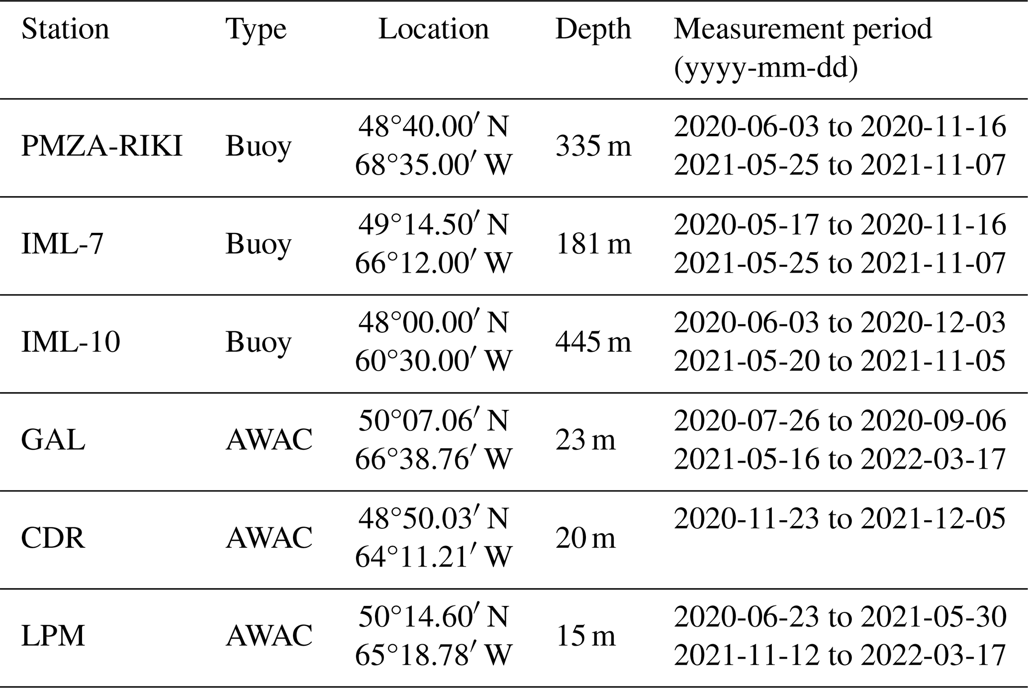
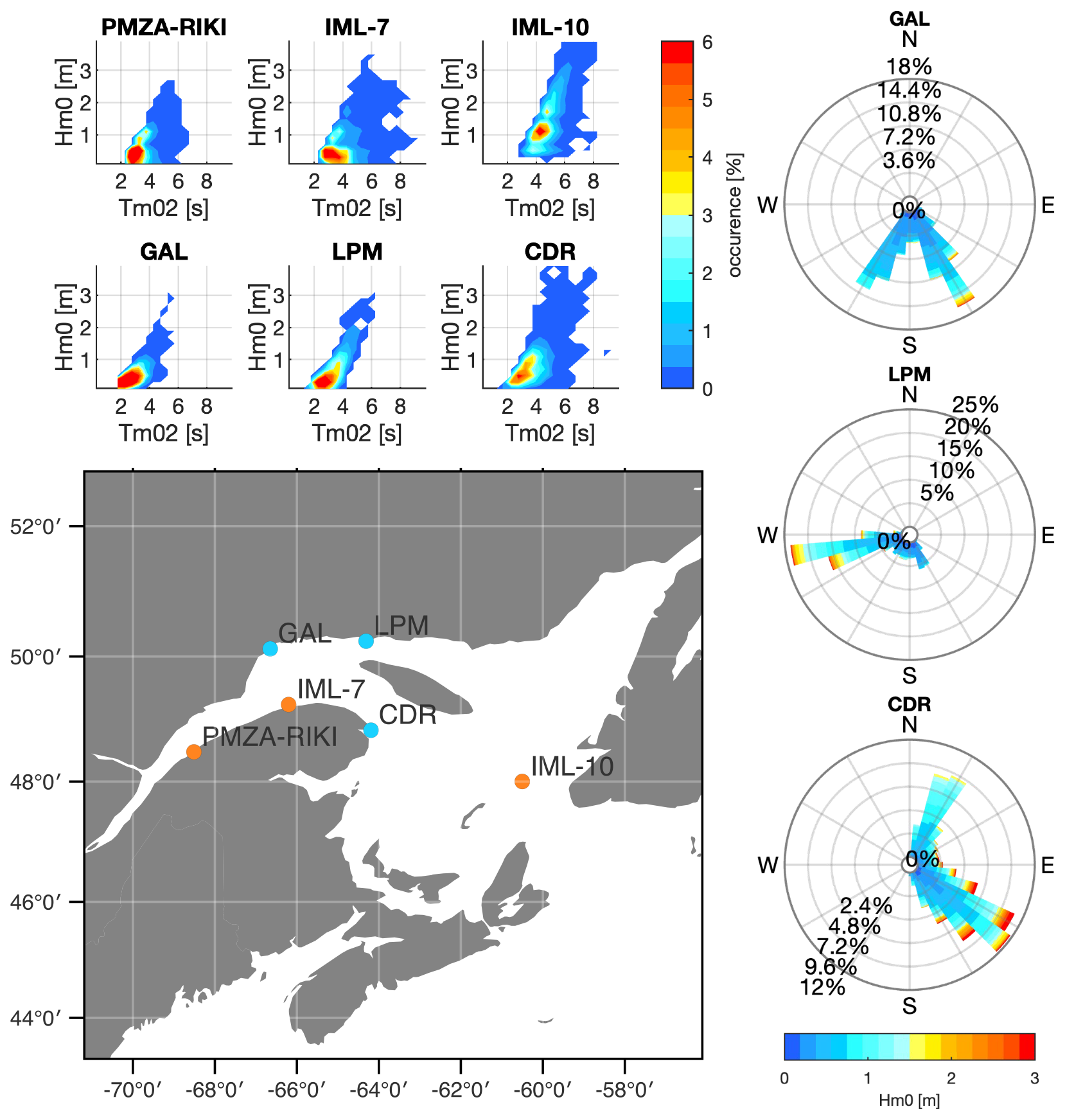
Figure 4 Analysis of the wave climate during the sampling period. Top panels show the joint distribution of significant height H_s and mean period T_m2 and right panels show the wave rose for the AWAC stations.

Since 1998, the Canadian Department of Fisheries and Oceans (DFO) has implemented the Atlantic Zone Monitoring Program (AZMP, Themault et al., 1998) to assess the oceanographic conditions in the EGSL, the Scotian Shelf as well as the Newfoundland and Labrador Shelf. As part of the program's sampling strategy, a network of multi-instrumented floating buoys is deployed and maintained since 2013. Buoys provide near-real-time wave observations (significant wave height H_s, mean wave period T_m02) every 30 min. Data are available through the St. Lawrence Global Observatory's (SLGO) marine conditions web application (https://ogsl.ca/conditions, last access: 20 August 2026). Buoys are temporarily recovered during winter to ensure maintenance and prevent damage related to the presence of sea ice. It is therefore not possible to assess wave forecasts performances during winter (December to May) using this dataset.

For more than a decade, the Chair in Coastal Geoscience at Université du Québec à Rimouski with the collaboration of the Quebec Minister of Public Security has undertaken a vast monitoring initiative to assess the hydrodynamic and morphodynamic conditions of the coastal waters of Quebec to characterize and map the coastal risks for the development of sustainable adaptation solutions (Bandet et al., 2020). This initiative includes the deployment of a network of directional and non-directional wave sensors. Here we use data from three 1 MHz Nortek Acoustic Wave and Current profilers (AWAC) deployed in intermediate to shallow waters that provide full directional spectra from which the mean wave direction can be extracted for analysis. Data were not accessible for real-time performance assessment but were instead added to the a posteriori performance analysis presented here.

The analysis of the sea state for the period of measurement is shown in Fig. 4. The joint distributions of significant wave height and mean wave period (Goda, 1978; Longuet-Higgins, 1983) show that the wave climate is mostly dominated by short period waves (∼ 2–3 s) associated with wave heights of 0.2–0.5 m. Because it is close to Cabot Strait, station IML-10 is influenced by the swell coming from the Atlantic and exhibits more energetic sea states dominated by waves with periods of 4–5 s.

4 System forecast skill assessment

Model performances are evaluated using data collected during a little less than 2 years (see Table 2). The dataset aggregates both data from the near-realtime verification system and data from the nearshore wave gauge network that have been processed a posteriori. Summer and winter periods are presented separately in order to assess the impact of the presence of sea ice on the accuracy of the prediction. Given that the focus is put on extreme sea states, results are presented for (i) all waves and (ii) values larger than the 90th percentile. The statistical parameters used in the study are defined in Appendix A.

4.1 Summer

In this section we use data collected between 31 March and 15 January to evaluate forecasts skills during the summer or ice-free period (see Figs. 6 and 7). Results of the statistical analysis are shown in Table 3.

Table 3 Model performance statistics with respect to the significant wave height H_s for the ice-free period (31 March to 15 January).

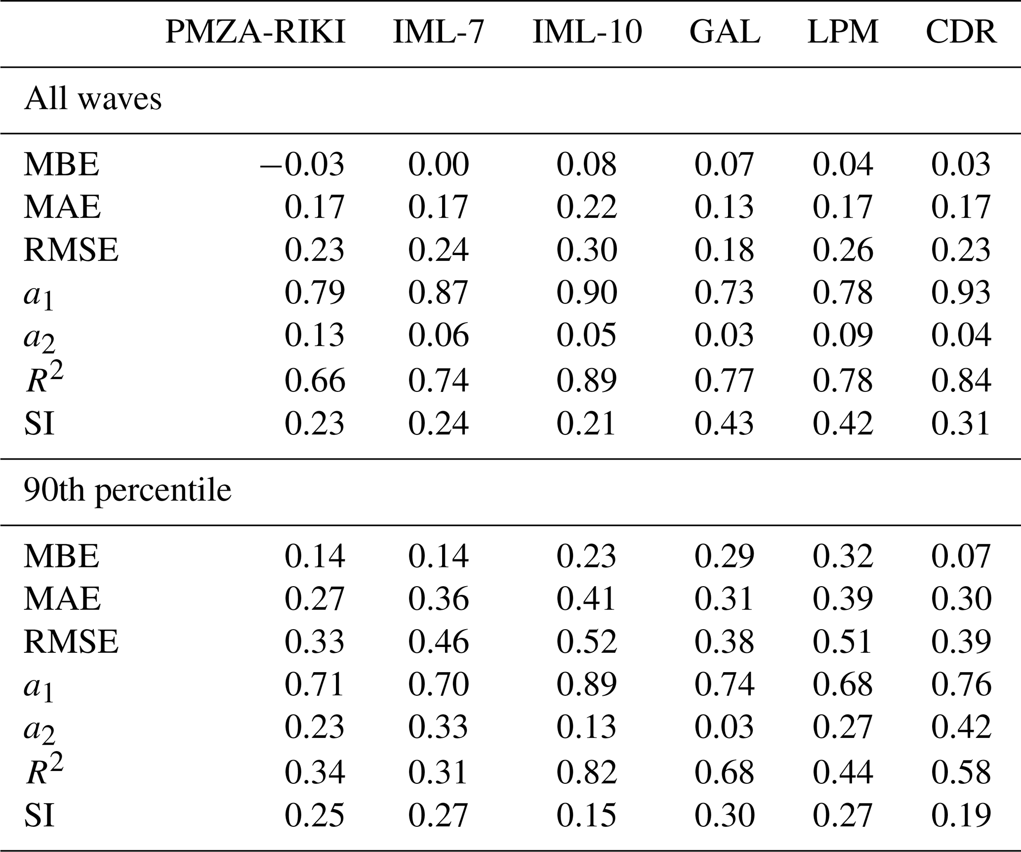
The analysis of significant wave height forecasts for +24 to +48 h lead times indicates that the system generally performs well throughout the EGSL. Across all wave conditions, the mean absolute error (MAE) ranges from 0.13 to 0.22 m, and the root mean square error (RMSE) varies from 0.18 to 0.30 m. This corresponds to a 21 % error relative to the average wave height observed at station IML-10 and 43 % at station GAL. Results show minimal bias, with the mean bias error (MBE) ranging from −0.03 to 0.07 m, and regression slopes a₁ between 0.73 and 0.93, suggesting that most errors are random rather than systematic.

When focusing on wave height values larger than the 90th percentile, the error represents only 15 % of the average wave height at IML-10 and 30 % at GAL. However, the bias increases slightly, with MBE values between 0.07 and 0.32 m, and regression slopes ranging from 0.68 to 0.89. This indicates a slight underestimation of the highest waves by the model.

As expected, the IML-10 station yields the most accurate results due to its offshore location in deep water (445 m depth), where it is directly influenced by Atlantic swell entering through the Cabot Strait. In contrast, the GAL station shows the largest discrepancies. Located in shallow water, its environment is characterized by the presence of sandbars that can move rapidly, altering the local bathymetry and influencing wave propagation, making accurate predictions more challenging.

The same statistical analysis was conducted for the mean wave period and mean wave direction. These results are presented in figures and tables of Appendix B. The analysis of the mean wave periods (Table B1) shows that these are generally well represented by the system with most of the data falling close to the 1:1 line. Nevertheless, predictions exhibit some degree of imprecision for all stations with a RMSE ranging from 0.69 to 1.06 s. This inaccuracy is associated with low-amplitude waves; when considering only the highest 10 % of waves, RMSE values drop between 0.59 and 1.0 s, corresponding to errors of 9 % to 21 % relative to the average period observed across stations. As with significant wave height, the IML-10 station exhibited the best performance levels.

The comparison of mean wave direction (Table B2) show a very good agreement between observations and forecasts. Results closely align with the 1:1 line with mean absolute error ranging between 18 and 27° for all waves. This error narrows to 15–19° for the 10 % of the highest waves indicating improved accuracy for more energetic sea states. The evaluation of system performances over the forecast lead time (Fig. 5) indicates that model accuracy remains consistent up to +48 h, with no significant degradation in the quality of the results over time. Although our configuration provided reasonably good results during the summer period, further improvements in forecast skills could be achieved with some adjustments. In particular, increasing the spectral frequency resolution may improve the representation of wave growth in the high-frequency range of the spectrum, especially during the development of wind seas following calm conditions (Soomere, 2005). Moreover, the use of alternative source term formulations for wind input and wave dissipation, such as ST4 or ST6, could potentially further enhance model performances (Lin et al., 2020).

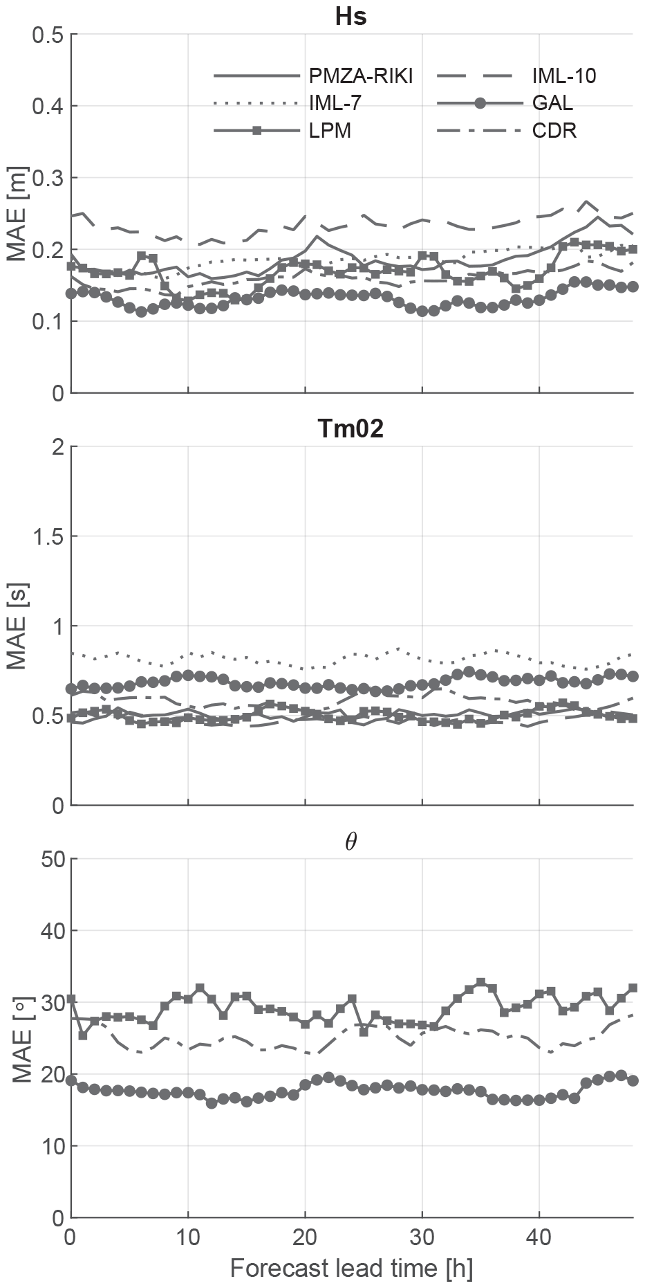
Figure 5 Mean absolute error (MAE) between observed and predicted wave parameters as a function of the forecast lead time for significant wave height (top), mean wave period (middle) and mean wave direction (bottom). Note that directional data are available only for stations GAL, LPM and CDR.

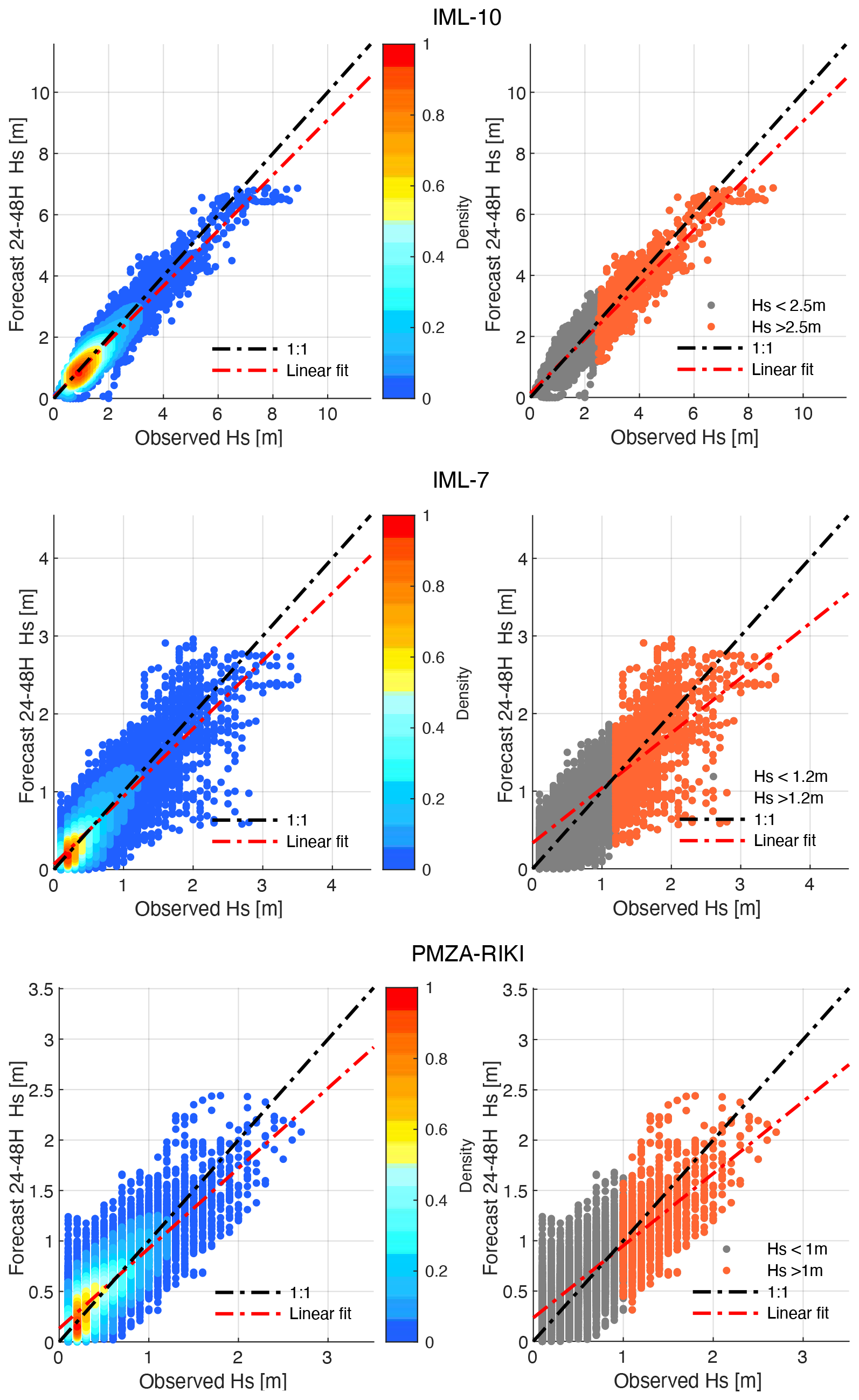
Figure 6 Scatter plot between observed and predicted significant wave height at the horizon 24–48 h for buoy stations IML-10, IML-7, PMZA-RIKI during the ice-free period (31 March to 15 January). The linear regression (orange dotted line) is applied to all waves on the left and to the highest 10 % waves on the right.

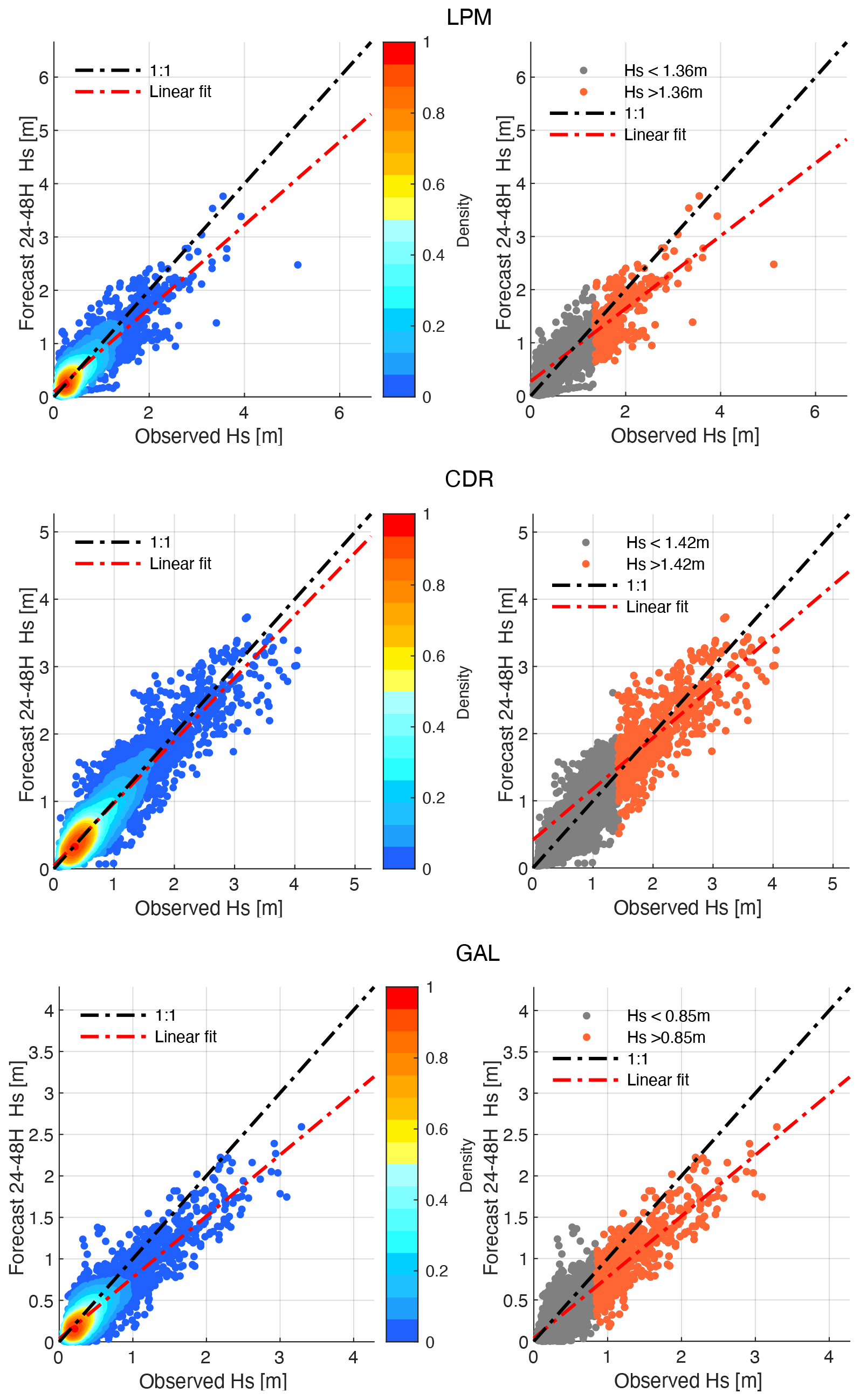
Figure 7 Scatter plot between observed and predicted significant wave height at the horizon 24–48 h for AWAC stations CDR, GAL and LPM during the ice-free period (31 March to 15 January). The linear regression (orange dotted line) is applied to all waves on the left and to the highest 10 % waves on the right.

4.2 Winter

Observations at stations LPM, CDR and GAL between 15 January and 31 March are used for assessing model skills during the winter period when the EGSL is partially covered by sea ice. Comparisons of significant wave height (Table 4, Fig. 8) show that the forecast skills are considerably reduced compared to the summer period. The model strongly underestimates the wave height when sea ice is present. The scatter index (SI, see Appendix A) exhibits errors of 88 % to 142 % of the average observed wave height. In CDR and GAL particularly, the model largely fails to represent the observed sea state, as shown by the slope of the regression line near 0 in GAL, and did not capture the most extreme events recorded during this period, associated with values exceeding 3 m. This poses a potential challenge for coastal hazard predictions in a seasonally ice-covered environment like the EGSL and emphasizes the critical need to improve wave-ice interactions for such application.

Table 4 Model performance statistics with respect to the significant wave height H_s for the winter ice-covered period (15 January to 31 March).

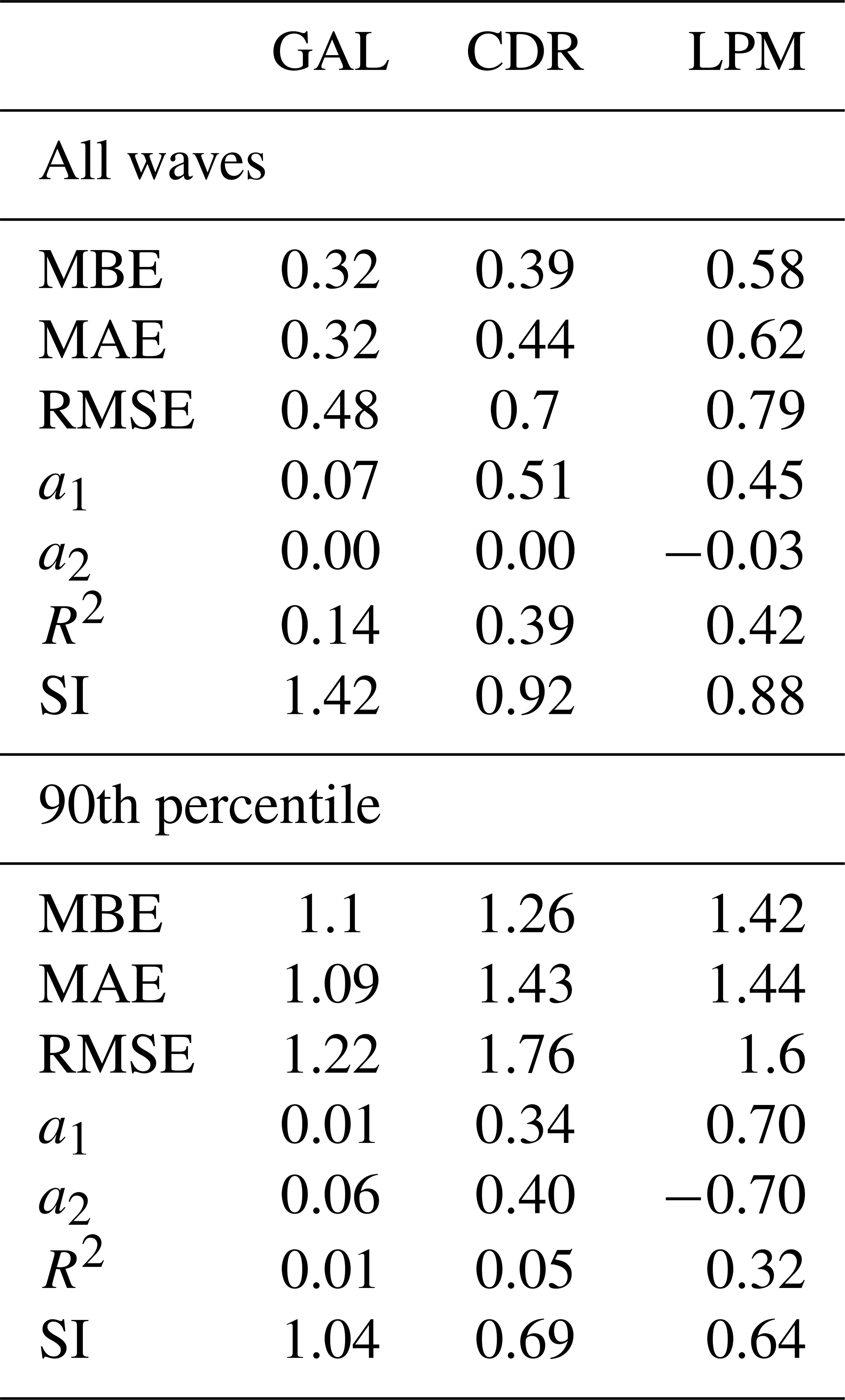
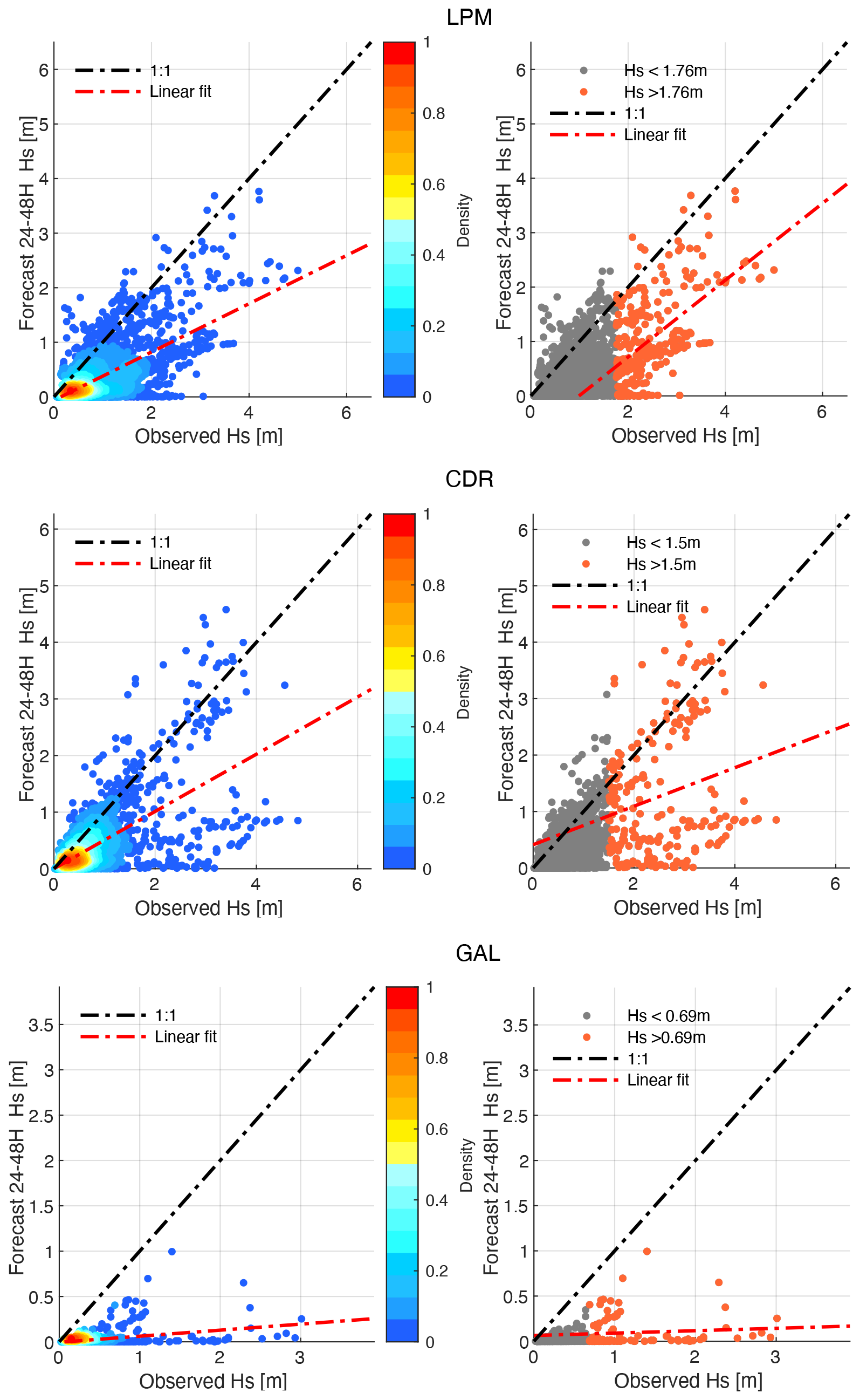
Figure 8 Scatter plot comparing observed and predicted significant wave height at the 24–48 h horizon for AWAC stations CDR, GAL, LPM during the ice-covered winter period (15 January–31 March). Left: all the waves, right: 90th percentile.

Multiple factors can hinder the model's ability to accurately predict the sea state in the presence of sea ice. Obviously, errors associated to the wave attenuation parameters, which is known to be highly heterogeneous (Stopa et al., 2018) is one important potential cause of error. There is a strong dependence of wave propagation on the ice mechanical properties (elasticity parameters and flexural failure thresholds) that depends on sea ice history (salt content, fractures, refreezing), which can be highly heterogeneous. As a result, the decay rate is a complex function of these properties, including thickness and floe size, rather than being solely based on the wave frequency. However, these parameters are rarely constrained concurrently with observations of wave attenuation rates and are still absent from empirical formulations.

But more essentially, our results underscores how critical the accuracy of the sea ice predictions is for such application. Indeed, the rate of wave energy decay in sea ice observed in the EGSL is $\mathcal{O}({\mathrm{10}}^{-\mathrm{3}}-{\mathrm{10}}^{-\mathrm{2}})$ m⁻¹. This means that – even with some degree of uncertainty on this value – waves with periods of 3–10 s (typical for the EGSL) will lose 75 % of their energy within just a few kilometers from the ice edge when the ice concentration is 1. That distance is in the order – if not smaller – of the spatial resolution of the sea ice model used in our system, as well as that of typical regional sea ice models. Consequently, even minor uncertainties over one or a few grid cells in the position of the ice edge or in the ice fraction can significantly increase the error at a given location and time (Tuomi et al., 2019), regardless of how well wave propagation in sea ice is represented in the wave model.

In Fig. 9, a snapshot of the predicted ice concentration is compared with satellite-derived observations from Sentinel-2 multispectral images (level 2A, accessed from Copernicus Services on 9 March 2021 at 15:16:49 UTC). Here, ice extent has been retrieved with a simple threshold-based algorithm using RGB (red-green-blue) and SWIR (Short-Wave Infrared) bands. The cloud coverage was first filtered by applying SWIR > 0.3 (SWIR being the average of bands b11 and b12) and pixels were flagged as sea ice when RGB > 0.3 (RGB defined as the average of bands b2, b3 and b4). Note that this procedure has not been developed and tested to be quantitatively accurate in a broad range of situations or used for automatic detection of sea ice, but only to analyse and interpret results obtained here. Sea ice concentration was then computed by binning the ice pixels on the same grid as the RDPS-CGSL model (5 km spatial resolution) for comparison. At the scale of the EGSL, spatial fields of satellite-derived and model ice concentration look (at least visually) quite similar with sea ice being mainly concentrated south of the GSL. At a finer scale however, the observed coverage is much more heterogeneous, the ice being stretched into streaks of dense concentration surrounded by open water. Figure 9h shows the evolution of wave energy along a transect through the observed and predicted ice field (with a constant attenuation coefficient of α = 10⁻³ m⁻¹). Results shows that all wave energy decay within the first 50 km when propagating across the model ice field while significant wave energy is still present after 100 km for the observed field. This simple analysis illustrates how the presence of structures at the submesoscale in the ice field affects significantly the wave propagation in the EGSL. Despite their significance, the physical mechanisms driving the emergence of these structures are still very poorly represented in continuum sea ice models. Specifically, the extent to which characteristics of the fragmented sea ice – such as the floe size distribution (FSD) – influence its mechanical behavior and its deformation in response to external stresses like wind, waves, and oceanic currents remains unclear (Boutin et al., 2021).

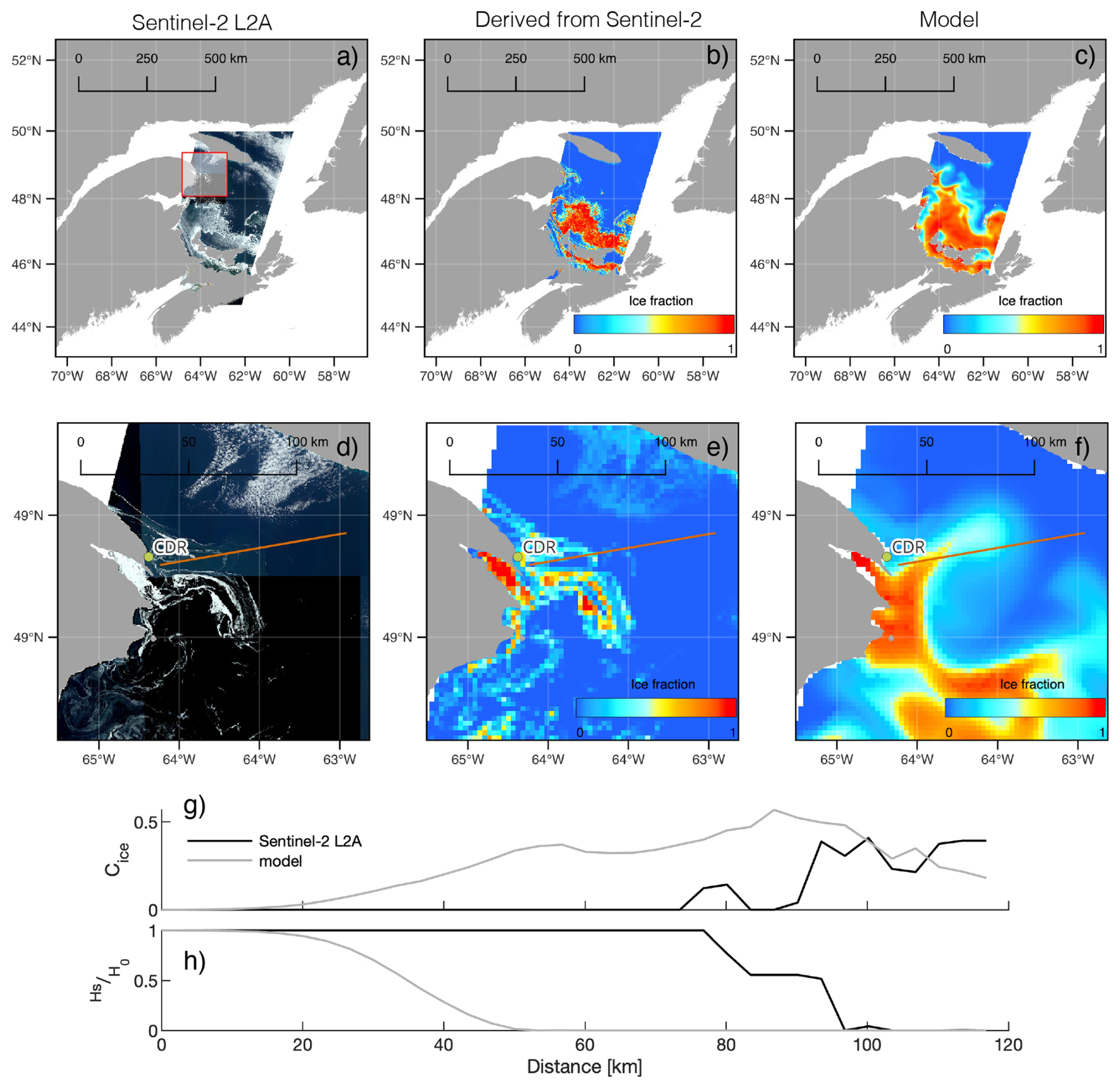
Figure 9 Comparison between satellite-derived (b, d) and model (c, f) ice concentration on 9 March 2021. Panels (g) and (h) are respectively the ice concentration and the corresponding wave energy attenuation along the orange transect.

The inherent granular and patchy nature of sea ice also raises the problem of dealing with unresolved subgrid-scale heterogeneity and nonlinear processes. Indeed, existing parameterizations of wave energy attenuation by sea ice often scale with the ice concentration and, in some cases, with ice thickness and floe size. Within a model grid cell, these properties are typically represented by bulk quantities (e.g. total ice fraction, mean thickness and mean floe size), therefore not retaining the sea ice spatial distribution and variability. From a mathematical perspective, if h_ice denotes the ice thickness, F the wave attenuation, which vary nonlinearly with h_ice, and the overbar denotes averaging, then $\stackrel{\mathrm{‾}}{F\left(h_{\mathrm{ice}}\right)}\ne F\left(\stackrel{\mathrm{‾}}{h_{\mathrm{ice}}}\right)$. These two terms are equal only if F is linear or weakly nonlinear, which is not the case for many wave attenuation parameterizations currently used in WW3. This is analogous to numerical weather prediction where subgrid spatial heterogeneity such as topography, land use, soil and vegetation characteristics affects significantly calculations of land-surface-atmosphere heat and momentum exchanges when highly nonlinear processes are involved (Giorgi and Avissar, 1997). Solutions to this long-standing problem have included the use of probability density functions (PDFs) to statistically represent heterogeneity (Avissar, 1992) or explicitly by partitioning grid cells into sub-grid tiles of homogeneous properties (Essery et al., 2003). In sea ice models such as CICE, subgrid-scale variability is accounted for using the floe size and thickness distribution (FSTD), which describes the fraction of the grid cell area covered by floes of a specific size and thickness. Incorporating FSTD into wave attenuation parameterizations could potentially lead to some improvements in modeling accuracy.

4.3 Extreme wave events: the case of Dorian

Comparisons conducted in the previous section highlight the global performances of the system under normal conditions. While several energetic conditions have been captured during the observation period, no extreme storm events leading to coastal hazards occurred. In order to evaluate the system performances under stormy conditions, we performed a hindcast run during the passage of the tropical storm Dorian, which hit the Gulf of St. Lawrence in September 2019 and caused severe damages across Atlantic Canada, especially in Nova Scotia, New Brunswick, Prince Edward Island and Magdalen Islands (Jardine et al., 2021; George et al., 2021).

The low pressure system originated off the west coast of Africa on 19 August 2019 before developing rapidly into a category 5 hurricane while hitting the Bahamas on 1 September. It further moved northeastward while weakening along the North American coast. The system then passed over the Gulf of St. Lawrence as a post-tropical storm with winds over 100 km h⁻¹ and gusts of 157 km h⁻¹ recorded at Wreckhouse Brook, Newfoundland (Avila et al., 2020). Water levels observed in Canada’s Maritime provinces were particularly affected. A storm surge of 1.85 m was observed at the Shediac tide gauge in New Brunswick. In Nova Scotia, the surge reached 1.22 m and resulted in water levels of 0.61 m above the higher high water large tide (HHWLT) level (the average of the water level annual maximum over a period of 19 years), approaching the historical record (Avila et al., 2020) and causing severe floods along the coast of the Prince Edward Island (Jardine et al., 2021).

The storm passed through the Magdalen Islands on 8 September. At that time, two Nortek AWACs were moored at two different locations along the coast of the islands, Baie de Plaisance (BDP) and Pointe aux Loups (PAL), recording hydrodynamical conditions during the storm (see Fig. 10). This dataset was used to evaluate the capabilities of the system to predict wave conditions during extreme events. Flood limits and maximum run-up extent were also assessed using field debris measurements conducted with GPS-RTK immediately after the storm passage. This dataset is used in the second part of this study to evaluate the ability of the system to predict the coastal TWL.

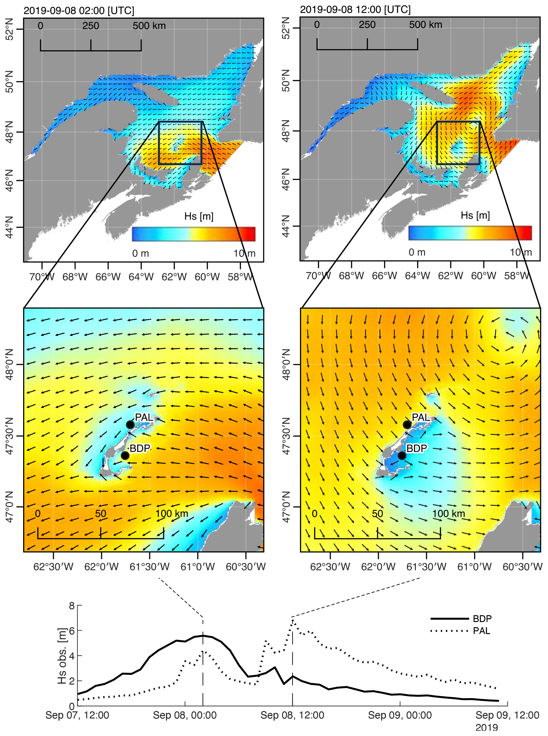
Figure 10 Top and middle panels show maps of the significant wave height H_s and mean wave direction predicted at the peak of the storm. The lower panel shows the evolution of H_s observed during the storm Dorian at Pointe aux Loups (PAL) and Baie de Plaisance (BDP).

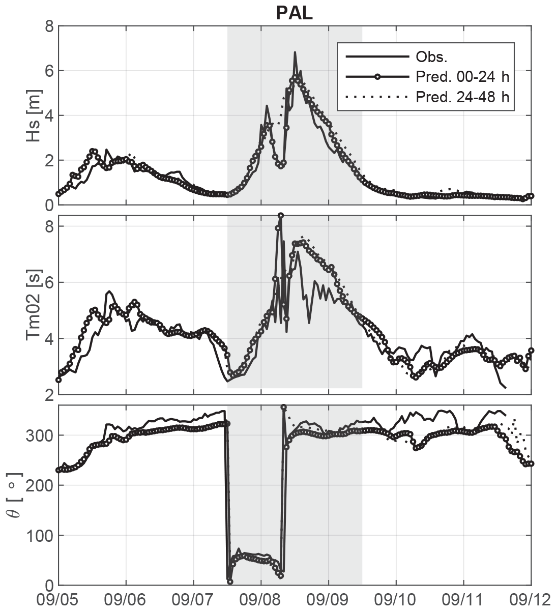
Figure 11 Comparison between observed and predicted time series of significant wave height H_s (upper panel), mean wave period T_m02 (middle panel) and mean wave direction θ (lower panel) at Pointe aux Loups during the storm Dorian (gray shaded area).

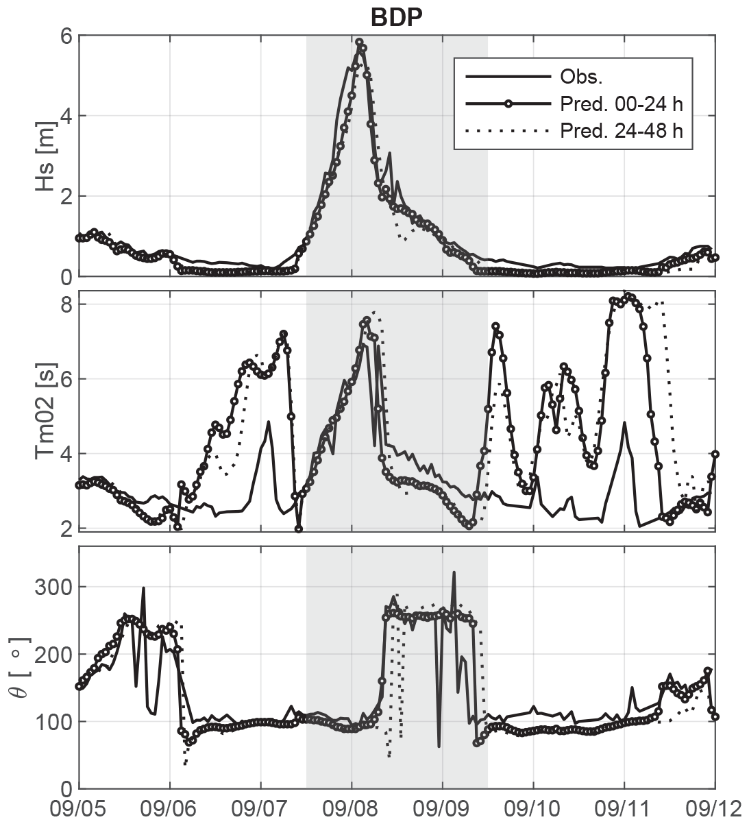
Figure 12 Comparison between observed and predicted time series of significant wave height H_s (upper panel), mean wave period T_m02 (middle panel) and mean wave direction θ (lower panel) at Baie de Plaisance during the storm Dorian (gray shaded area).

The maximum significant wave height recorded at Baie de Plaisance during Dorian reached 5.58 m at 02:00 UTC on 8 September and 6.82 m at Pointe aux Loups 10 h later, both associated with periods of ∼ 7.5 s. Figure 10 shows the predicted wave field at +48 h lead time for these two particular times. Figures 11 and 12 present the comparison of the significant wave height H_s, mean period T_m02 and mean direction θ time series observed and predicted by the system for the 0–24 and 24–48 h lead time windows. Forecasts show a very good agreement with the observations for all three wave parameters. Both amplitude and the timing of the storm peak are well captured by the model. There are also very few discrepancies between 0–24 and 24–48 h forecasts. Note however that before and after the passage of the storm at Baie de Plaisance, the system demonstrates a poor ability to represent the period of very low amplitude waves (< 0.2 m). Evaluation of wave models performances under extreme conditions have been carried out many times, with mixed outcomes (Campos and Guedes Soares, 2016; Myslenkov et al., 2021; Bertotti et al., 2012). Best results often involved de-biasing wind fields and calibrating parameters values for wind generation source terms S_in (Campos et al., 2018). In our case, we kept the default parameter values for the wind generation/dissipation source terms and used HRDPS U₁₀ as provided by ECCC without any de-biasing or calibration process. It confirms therefore that wind forcing accuracy is a major determinant of wave prediction skills and the importance of having access to high resolution, reliable wind forecasts in order to accurately predict extreme sea states. These results are very encouraging and show that this wave model configuration provide robust and reliable wave forecasts for further use in storm hazard prediction.

5 Conclusions

This study describes a 1 km high-resolution WW3 configuration that was implemented as part of a coastal hazard prediction system for the Estuary and Gulf of St. Lawrence (EGSL). The region is notably characterized by short fetch and presence of seasonal sea ice that affect the wave climate during winter. Model performances are assessed against field observations collected over a 2-year period and a distinction is made between winter and summer periods to account for the presence of sea ice in the accuracy of the predictions. Since the wave model is dedicated to coastal hazard forecasting, an emphasis is put on the ability of the system to simulate energetic conditions – i.e. the highest 10 % waves.

A key finding of the study is the significant difference in forecast skill between the summer ice-free season and the winter period, during which sea ice exerts a dominant influence on the wave climate. While the system performs reasonably well in summer especially for the most energetic sea states, it consistently underestimates waves during winter. In the EGSL, the ice cover is mainly composed of a mixture of brash ice and thin consolidated, highly mobile ice floes of size ranging from approximately 1 to 100 m. At the spatial scales over which waves with periods of 3 to 10 s typically dissipate 𝒪(1−10) km, the sea ice distribution is often highly heterogeneous. Driven by wind, oceanic flows such as fronts and eddies and wave radiation stress, sea ice tends to gather in streaks and filaments creating alternating areas of dense ice aggregates and open water. The dynamic of this fragmented sea ice is still poorly represented in current continuum sea ice models, resulting in significant inaccuracies in predicted ice fields at the spatial scales relevant to resolve wave propagation and attenuation. Recent improvements made to sea ice source terms within current wave models (Collins and Rogers, 2017) have therefore limited value unless accompanied by the implementation of a suitable rheology for fragmented sea ice and the development of coupled wave–ice-ocean modelling framework that account for the multiples feedback mechanisms between waves and sea ice – such as wave breaking, attenuation, and radiation stress. However, many ongoing researches are moving in this direction, both from an ocean wave perspective (Thomson, 2022) and sea ice perspective (Dumont, 2022) including coupling efforts (Boutin et al., 2021). A complementary avenue for improving operational wave forecasting in ice-infested waters is the development of sea ice ensemble prediction systems (Peterson et al., 2022; Röhrs et al., 2023) which may allow to better characterize the large uncertainties associated with sea ice conditions. In the context of a coastal hazard prediction system, an ensemble approach may even be more suitable than a purely deterministic approach, as from a risk management point of view, quantifying forecast uncertainty is arguably as important as the predicted value itself. However, existing sea ice ensemble prediction systems primarily account for uncertainties arising from atmospheric forcing and initial conditions (Nakanowatari et al., 2022; Röhrs et al., 2023), while uncertainties associated with sea ice mechanical properties remain not represented, which generally leads to ensembles being highly underdispersive (Strommen et al., 2026).

Hindcast performed during the post-tropical storm Dorian exhibits strong accordance with observations both in terms of amplitude of the incoming waves and timing of the peak of the storm. This result is particularly promising, as it demonstrates the system's ability to accurately capture extreme events that may lead to coastal hazards. Overall, results obtained in the first part of this study demonstrate that a regional high-resolution WW3 configuration forced by current atmospheric and oceanic forecasts provided by ECCC is able to deliver reliable short-term predictions of the sea state. This configuration provide a solid foundation to estimate the contribution of ocean waves to the TWL within a coastal hazard prediction system. Nonetheless, enhancing accuracy during winter will require improvements toward a fully coupled ocean–wave–ice modelling framework. The second part of the study focuses on the estimation of TWL using semi-empirical formulations for wave set-up and run-up, and provide a thorough examination of system performances using observations of TWL.

Appendix A: Statistical and skill assessment metrics

In this section, the statistical and skill assessment parameters used to evaluate model performances are described. In the following, O_i and P_i denote the predictions and observations and the overbar denotes the mean such that $\stackrel{\mathrm{‾}}{O}$ = $\frac{\mathrm{1}}{n}\sum _{i=\mathrm{1}}^n{O}_i$.

A1 Statistics for non-directional data

A1.1 Mean Bias Error (MBE)

The mean bias error is defined as

$$\begin{array}{}\text{(A1)}& \text{MBE}={\displaystyle \frac{\mathrm{1}}{n}}\sum _{i=\mathrm{1}}^n{O}_i-P_i\end{array}$$

and indicates the average deviation between variables O and P, i.e. the tendency to overestimate or underestimate one relative to the other. It is a dimensional parameter (same units as O and P). The ideal value is 0.

A1.2 Absolute mean error (MAE)

$$\begin{array}{}\text{(A2)}& \text{MAE}={\displaystyle \frac{\mathrm{1}}{n}}\sum _{i=\mathrm{1}}^n|O_i-P_i|\end{array}$$

The absolute bias indicates the magnitude of the error between variables O and P. It is a dimensional parameter (same units as O and P). The ideal value is 0.

A1.3 Root mean square error (RMSE)

The root mean square error is given by

$$\begin{array}{}\text{(A3)}& \text{RMSE}=\sqrt{{\displaystyle \frac{\mathrm{1}}{n}}\sum _{i=\mathrm{1}}^n(O_i-P_i{)}^{\mathrm{2}}}.\end{array}$$

Like the MAE, it is an indication of the magnitude of the error but gives more weight to extreme values. It is a dimensional parameter (same units as O and P). The ideal value is 0.

A1.4 Scatter index (SI)

The scatter index is here defined as the RMSE normalized by the observational mean, such that

$$\begin{array}{}\text{(A4)}& \text{SI}={\displaystyle \frac{\text{RMSE}}{\stackrel{\mathrm{‾}}{O}}}.\end{array}$$

Lower values of SI indicate a better model performance.

A1.5 Linear regression coefficients

Suppose there exists a linear relationship between variables O and P, it is possible to apply a linear regression model such that

$$\begin{array}{}\text{(A5)}& \widehat{P}=a_{\mathrm{1}}O+a_{\mathrm{2}}\end{array}$$

and

$$\begin{array}{}\text{(A6)}& P=\widehat{P}+\mathit{ϵ}\end{array}$$

where a₁ and a₂ are the slope and offset coefficients of the linear regression obtained with the least mean square method and obtained as

$$\begin{array}{}\text{(A7)}& a_{\mathrm{1}}={\displaystyle \frac{{\sum }_{i=\mathrm{1}}^n(P_i-\stackrel{\mathrm{‾}}{P})(O_i-\stackrel{\mathrm{‾}}{O})}{{\sum }_{i=\mathrm{1}}^n(O_i-\stackrel{\mathrm{‾}}{O}{)}^{\mathrm{2}}}}\end{array}$$

and

$$\begin{array}{}\text{(A8)}& a_{\mathrm{2}}=\stackrel{\mathrm{‾}}{P}-a_{\mathrm{1}}\stackrel{\mathrm{‾}}{O}\end{array}$$

where $\stackrel{\mathrm{‾}}{P}=\frac{\mathrm{1}}{n}{\sum }_{i=\mathrm{1}}^n{P}_i$ and $\stackrel{\mathrm{‾}}{O}=\frac{\mathrm{1}}{n}{\sum }_{i=\mathrm{1}}^n{O}_i$ are the empirical mean of P_i and O_i, respectively.

The slope coefficient a₁ is an adimensional parameter that gives an indication about the bias trend, while a₂ has the same units as P and O and indicates an offset between the two. The ideal values are a₁ = 1 and a₂ = 0.

A1.6 Coefficient of determination (R²)

The coefficient of determination is defined as

$$\begin{array}{}\text{(A9)}& R^{\mathrm{2}}={\left({\displaystyle \frac{{\sum }_{i=\mathrm{1}}^n(O_i-\stackrel{\mathrm{‾}}{O})(P_i-\stackrel{\mathrm{‾}}{P})}{{\sum }_{i=\mathrm{1}}^n(O_i-\stackrel{\mathrm{‾}}{O}{)}^{\mathrm{2}}{\sum }_{i=\mathrm{1}}^n(P_i-\stackrel{\mathrm{‾}}{P}{)}^{\mathrm{2}}}}\right)}^{\mathrm{2}}\end{array}$$

and indicates the fraction of the total variance that is explained by the linear regression. Its ideal value is 1.

A2 Statistics for directional data

In what follows, O and P are angles expressed in degrees.

Directional mean absolute error (MAE)

The mean absolute error for directions is equivalent to the mean absolute bias for dimensional scalar values and is computed as

$$\begin{array}{}\text{(A10)}& \text{MAE}={\displaystyle \frac{\mathrm{1}}{n}}\sum _{i=\mathrm{1}}^n{D}_i\end{array}$$

where

$$\begin{array}{}\text{(A11)}& D_i=\left\{\begin{array}{ll}|O_i-P_i|& \text{si}\mathrm{0}<|O_i-P_i|\le \mathrm{180}\\ \mathrm{360}-|O_i-P_i|& \text{si}\mathrm{180}<|O_i-P_i|\le \mathrm{360}\end{array}\right.\end{array}$$

Appendix B: Model skill with respect to wave period and direction

Tables B1 and B2 presented in this appendix report skill assessment parameter values for wave period and direction, respectively.

Table B1 Model performance statistics with respect to the mean wave period T_m02 (in seconds) for the ice-free period (31 March to 15 January).

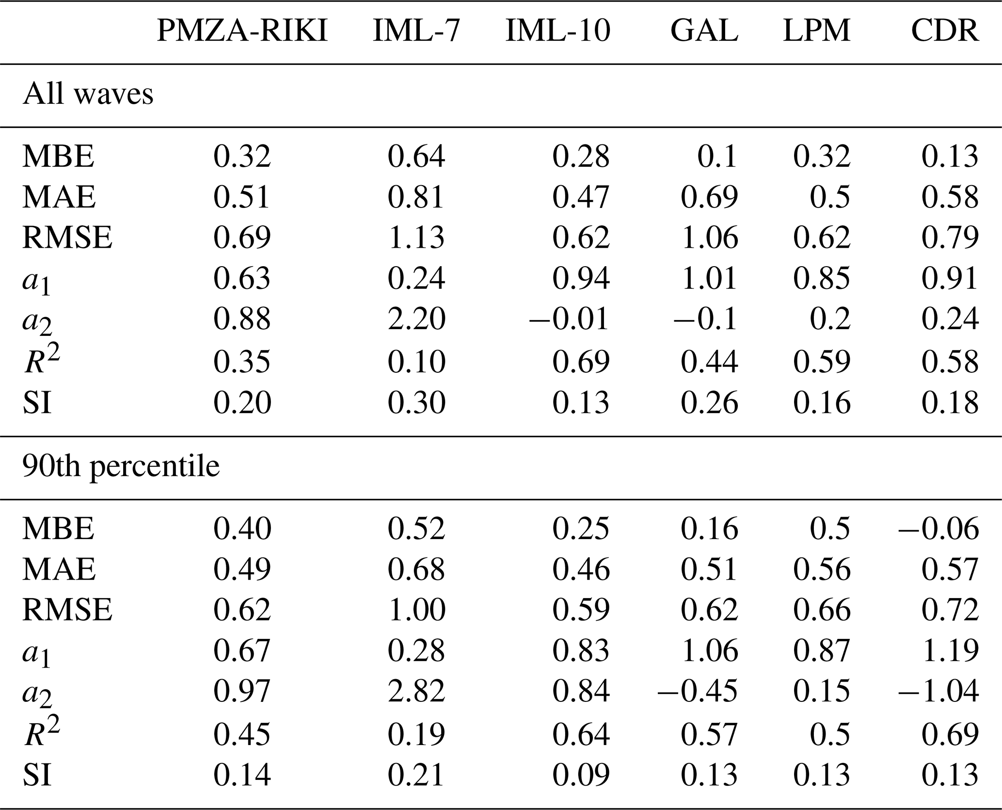
Table B2 Model performance statistics with respect to the mean wave direction θ (in degrees) for the ice-free period (31 March to 15 January).

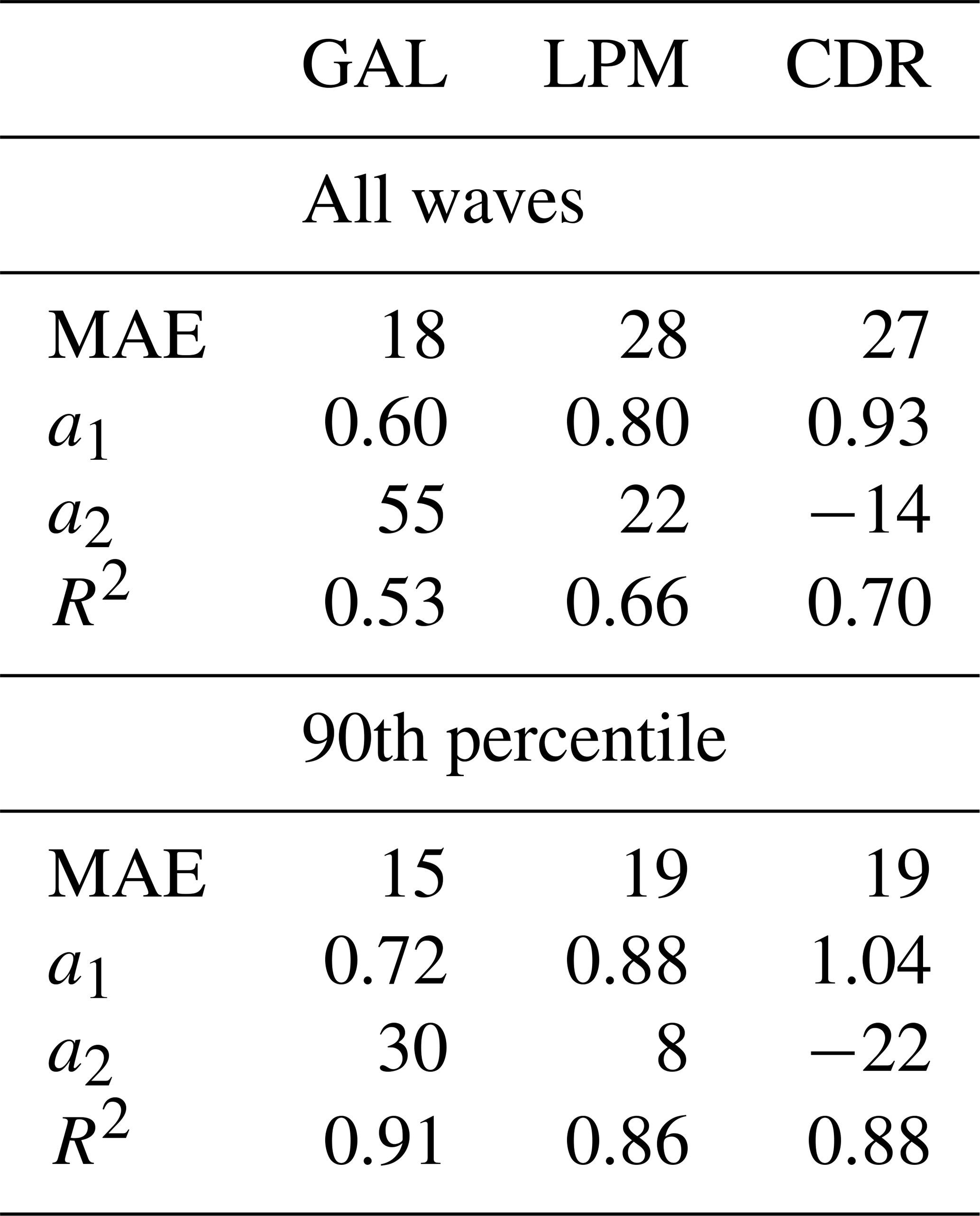
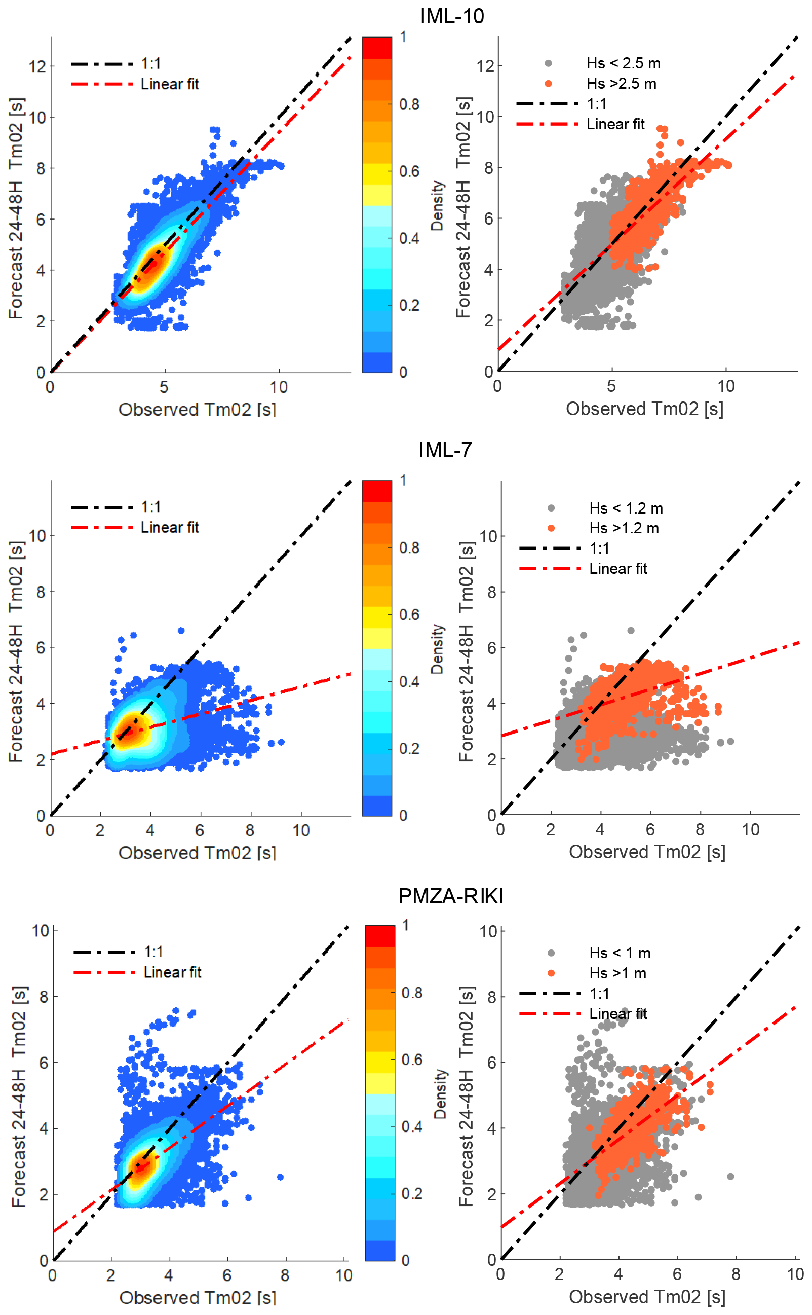
Figure B1 Scatter plot comparing observed and predicted mean wave period at the horizon 24–48 h for buoy stations IML-10, IML-7, PMZA-RIKI during the ice-free period (31 March to 15 January). The linear regression (orange dotted line) is applied to all waves on the left and to the highest 10 % waves on the right.

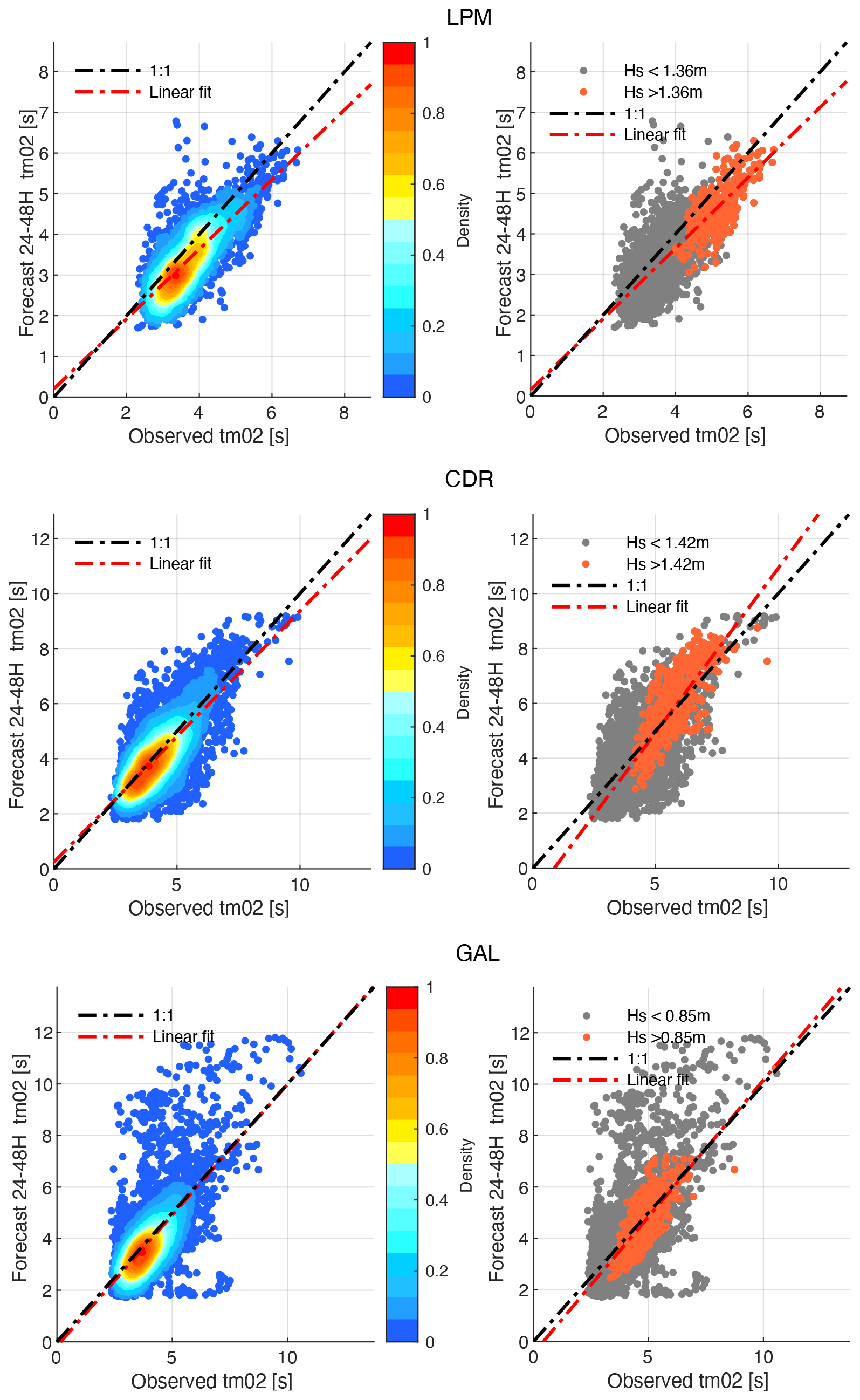
Figure B2 Scatter plot comparing observed and predicted mean wave period at the horizon 24–48 h for AWAC stations CDR, GAL and LPM during the ice-free period (31 March to 15 January). The linear regression (orange dotted line) is applied to all waves on the left and to the highest 10 % waves on the right.

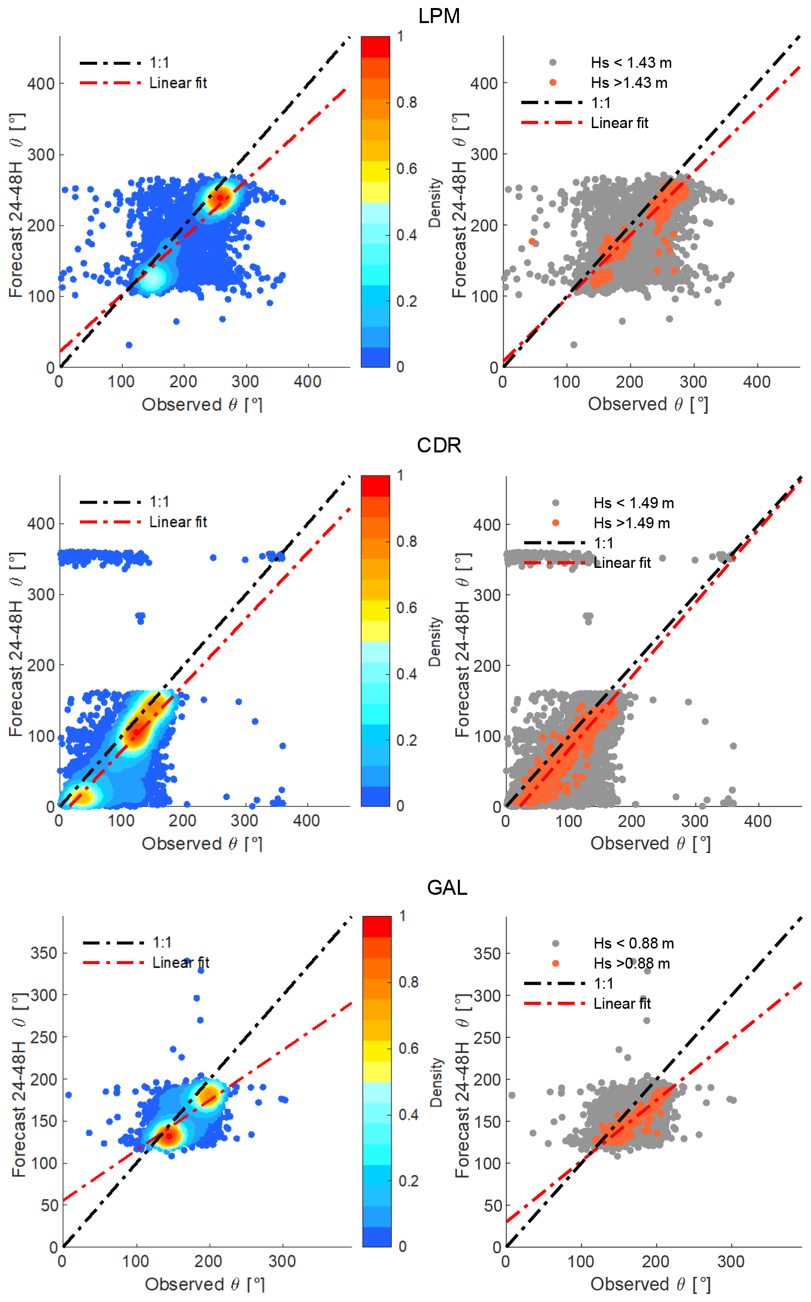
Figure B3 Scatter plot comparing observed and predicted mean wave direction at the horizon 24–48 h for AWAC stations CDR, GAL and LPM during the ice-free period (31 March to 15 January). The linear regression (orange dotted line) is applied to all waves on the left and to the highest 10 % waves on the right.