Modeling the combined effects of the 2023 Türkiye–Syria earthquake and an Atmospheric River event on landslide hazard

The 6 February 2023 Türkiye–Syria earthquake doublet triggered thousands of coseismic landslides. On 14–15 March, an Atmospheric River (AR) delivered up to 183 mm of rainfall across the seismically weakened region, triggering hundreds of additional landslides and debris flows, causing extensive downstream flooding and damage. Existing regional hazard assessment tools typically model seismic- and rainfall-triggered landslides separately, and rarely incorporate post-seismic hillslope weakening into rainfall-based predictions. Here, we develop a rapidly deployable regional hazard model that integrates seismic and rainfall drivers with post-seismic legacy effects to map landslide probability using the open-source Landlab framework and global gridded datasets. Incorporating legacy effects improves model performance under the AR forcing, yields more realistic probabilities, and lowers the critical slope for landslide initiation by up to 13° relative to the same model without the legacy effect. Analysing event sequencing, we find that this AR event preceding or coincident with the earthquake produces the greatest hazard extent, with median critical slopes in high-probability areas (P(F)≥0.6) up to 7° lower than when the AR follows the seismic event. Finally, we develop a pre-event forecasting method that uses historical extreme rainfall records to map post-seismic landslide hazard and show that it closely replicates the hazard map derived from the 14–15 March AR event. The proposed model supports disaster preparedness, early warning, and risk reduction before and after earthquakes in landslide-prone regions.

1 Introduction

Ground shaking from strong earthquakes can trigger coseismic landslides, often concentrated on steep slopes and near hillcrests where shaking is amplified by topography (Meunier et al., 2008, 2013; Marc et al., 2016). Coseismic landslides mark the beginning of a chain of cascading earthquake hazards (CEHs), including debris flows, mudflows, and sedimentation in streams. Landscapes may remain susceptible to such secondary earthquake hazards for months and even years after the initial seismic event (Fan et al., 2019).

A key element of CEH is the continued supply of sediment from hillslopes after major shocks. Following earthquakes, hillsides become more susceptible to landslides due to topographic change, soil/rock fractures, damage to vegetation, and altered soil hydrologic and geotechnical properties (Leshchinsky et al., 2021; Xi et al., 2024a; Brain et al., 2017). These “earthquake legacy” effects often lower rainfall thresholds for landslide initiation, resulting in elevated landslide rates during the post-seismic period compared to the pre-seismic phase (Lin et al., 2004; Zhang and Zhang, 2017). Elevated landslide rates and sediment export from earthquake-affected areas can persist for months to years (Tanyaş et al., 2021a), and are generally highest in regions with high topographic relief, seasonally varying rainfall, and substantial coseismic deposits (Fan et al., 2019; Tanyaş et al., 2021b). Conversely, extreme rainfall can shorten this elevated-hazard period by rapidly exporting large amounts of sediments from the earthquake-affected zone (Lenti and Martino, 2013; Brain et al., 2021; Brain et al., 2017).

Many examples of CEHs have been reported in the literature. For example, monsoon rainfalls following the 2015 Gorkha earthquakes produced more landslides than similar rainfalls in the pre-seismic period (Jones et al., 2021; Kincey et al., 2023; Burrows et al., 2023). After the Chi-Chi earthquake in Taiwan, sediment yields peaked above five times the background rates, gradually returning to pre-earthquake levels in 6 years (Hovius et al., 2011). A decade after the 2008 Wenchuan earthquake, which had a long recovery period due to large amounts of coseismic deposits, about 88 % of the deposits remained on hillsides (Francis et al., 2022; Tanyaş et al., 2021a). Coseismic deposits may also exacerbate flood hazards under heavy rainfall. Two years after the 2008 Wenchuan earthquake, heavy rainfall remobilized sediments accumulated from coseismic landslides in the foothills and mountain terraces. Aggradation of these sediments in river channels reduced the conveyance capacity of rivers, causing extensive flooding hazards (Hairong et al., 2017; Huang and Fan, 2013; Liu and Yang, 2015).

Some extreme combinations of these factors converged in the aftermath of the 6 February 2023 Türkiye–Syria earthquake doublet (M_w 7.8 and M_w 7.5) along the East Anatolian Fault Zone (Fig. 1), which triggered more than 3600 coseismic landslides (Görüm et al., 2023). On 14–15 March 2023, a rare Atmospheric River (AR) event caused extreme rainfall in the central part of the earthquake-affected region, delivering up to 183 mm rain over 2 d at some locations (Fig. 2). This extreme rainfall triggered secondary landslides and debris flows in the source areas, and flooding in downstream communities, causing a major disruption in earthquake recovery efforts, damage to temporary shelters, and life loss (Görüm et al., 2025). In Southeastern Türkiye, the frequency and intensity of AR events have increased in recent decades specifically during the cold season, particularly in late winter and early spring when snowmelt conditions prevail and soils are already saturated, heightening the risk of runoff-induced hazards (Bozkurt et al., 2021; Görüm et al., 2025). This pattern is not unique to Türkiye; other seismically active regions, particularly around the Pacific Rim, are also projected to experience increases in AR intensity and frequency (Warner et al., 2015; Wang et al., 2023). However, earthquake hazard assessment protocols do not adequately account for earthquake legacy effects or represent compound seismic and rainfall drivers of landslides (Görüm et al., 2025).

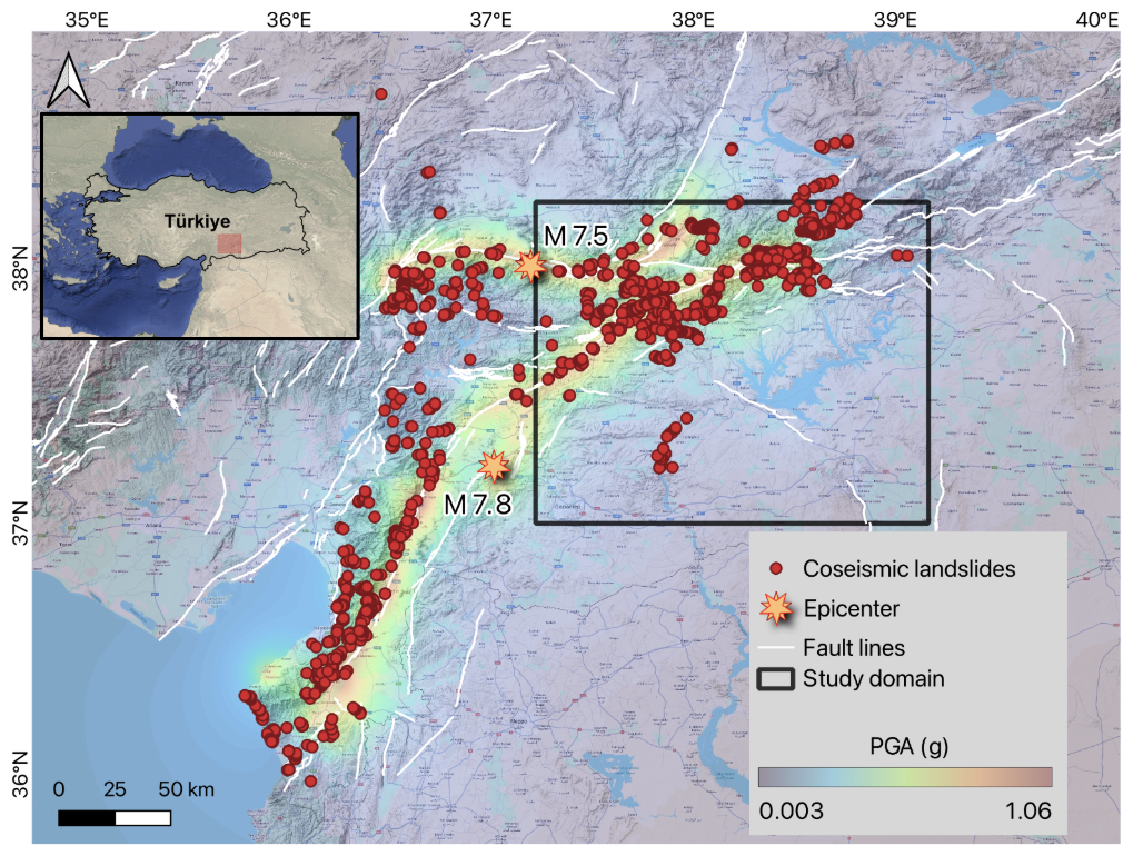
Figure 1 USGS ShakeMap raster composition which consists of PGA resulting from the two major earthquakes of magnitude M_w 7.8 and M_w 7.5 (exclusive of aftershocks) occurring along the East Anatolian fault zone. The coseismic landslide inventory, marked by red circles, is provided by Görüm et al. (2023), while the active faults, indicated by white lines, are mapped by Emre et al. (2013). ShakeMap PGA data © USGS. Active fault data © MTA (General Directorate of Mineral Research and Exploration, Türkiye).

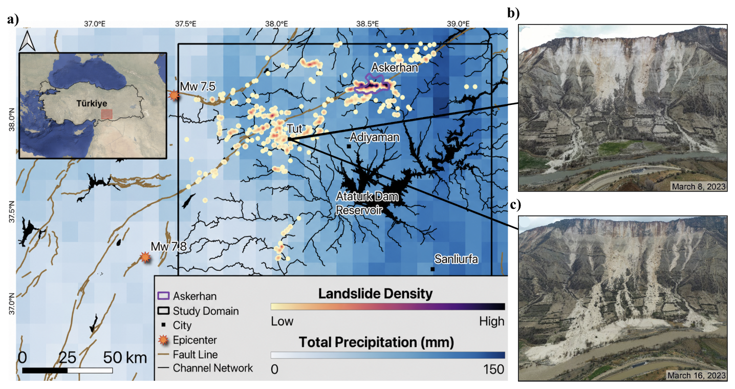
Figure 2 (a) NASA's Integrated Multi-satellitE Retrievals for GPM (IMERG) precipitation estimates for 10–16 March 2023. This atmospheric river swept through the central earthquake impacted area, delivering up to 146.4 mm of rainfall over a 7 d span. Photos captured within the town of Tut illustrate the landscape effects of (b) coseismic driven crown cracking and landsliding and (c) post-seismic storm-driven sedimentation and debris flow (Görüm et al., 2025). A 10 km² validation site within the Askerhan subcatchment, where a high density of post-seismic landslides were observed, was selected for model validation. IMERG precipitation data © NASA.

Research on earthquake legacy effects on slope stability has produced both detailed process-based formulations and simpler empirical approaches. Detailed models can represent strength loss through changes in effective cohesion, internal friction, root reinforcement, deformation, and evolving failure geometry by explicitly simulating stress–strain behavior, hydromechanical coupling, and, in some cases, seismic forcing (Jibson, 2011; Duncan, 1996; Griffiths and Lane, 2001; Leshchinsky et al., 2021). However, these models are generally data- and computation-intensive and are often limited to site-specific research applications (van den Bout et al., 2022; Chen et al., 2023). At the regional scale, Xi et al. (2024a, b) proposed an empirical relationship linking reduction in shear strength (RSS) to peak ground acceleration (PGA), showing that coseismic hillslope weakening can be represented in a transferable way across multiple earthquake settings.

Coseismic landslide hazard models similarly range from more complex dynamic and numerical slope-stability formulations to simplified Newmark sliding-block displacement models and their probabilistic and machine-learning (ML) extensions. More complex approaches can represent coupled soil response, progressive failure, internal deformation, and evolving landslide geometry during shaking, including dynamic soil-column formulations, simplified physics-based numerical models, and pseudo-3D analyses that relax the assumption of predefined planar failure surfaces (Wartman et al., 2003; Berrett et al., 2025; Gong et al., 2023). At regional scales, however, many applications still rely on Newmark-based models, which extend slope-stability analysis to estimate coseismic displacement and are computationally efficient and adaptable to probabilistic mapping, including logic-tree and displacement-hazard formulations, as well as hybrid ML applications (e.g., Wang and Rathje, 2015; Li et al., 2022; Zhang et al., 2025; Peláez et al., 2025). However, hydrologic forcing is often oversimplified in coseismic landslide hazard predictions. Most applications either neglect soil-water effects by assuming dry or prescribed saturation states (Wang and Rathje, 2015; Li et al., 2022; Gong et al., 2023; Djukem et al., 2024) or, even when subsurface flow is represented explicitly, do not adequately resolve antecedent soil moisture and root-zone water-balance dynamics (e.g., Zhang et al., 2025; Nguyen et al., 2024; Zeng et al., 2025). These limitations point to the need for rapidly deployable regional models that forecast post-seismic, rainfall-driven hazards under earthquake legacy effects and capture the sequencing of seismic and rainfall drivers.

Here we formulate such a modeling approach for shallow landslides and address the following questions in the study domain located in the northeastern portion of the earthquake-affected region of Türkiye (Fig. 2). (1) How can a regional landslide hazard model integrate seismic and rainfall drivers and earthquake legacy effects by leveraging global gridded data products? (2) How does the sequence of extreme seismic and rainfall drivers influence landslide hazards? (3) How can we develop a pre-event forecasting approach of post-seismic rainfall-driven landslide hazards in advance of future extreme precipitation events? The models presented in this research are developed using the open-source Landlab earth surface modeling framework (Hobley et al., 2017). Global remote sensing products inform model parameters, climate and seismic forcings, and limited hydrologic model confirmation, enabling deployment in data-scarce or rapid-response settings, where local ground measurements may be unavailable.

This study includes three groups of analyses. First, to address question 1, we present the modeled hydrologic response to the 14–15 March AR event and the resulting post-seismic landslide hazard with and without earthquake legacy effects, parameterized as a function of the Peak Ground Acceleration (PGA) following Xi et al. (2024a). These results are corroborated with satellite-derived soil moisture and mapped landslides. Second, we analyze how rainfall-earthquake sequencing influences spatial patterns of coseismic landslide hazard and compare these results with post-seismic legacy model (question 2). Finally, in response to question 3, we illustrate our pre-event forecast approach for post-seismic, rainfall-driven landslide hazards using historical satellite-derived precipitation together with earthquake legacy effects and compare the resulting hazard map with that derived from the 14–15 March AR event. By relying on historical extremes rather than real-time rainfall observations, this approach enables forecasting of high-risk zones before extreme precipitation events, supporting early warning and mitigation efforts.

2 Study site and event context

The model is applied to a study area in the north-central and eastern parts of the earthquake-impacted area, covering the towns of Tut, Adiyaman and Sanliurfa that were impacted from an AR driven extreme rainfall event between 14–16 March (Fig. 2). The mountains in the northern part of the study domain mark the highest elevations within the earthquake region and deliver sediment to the tributaries of the Euphrates river and the Atatürk Dam Reservoir. These physiographic differences are accompanied by considerable climatic variability across the region.

Climate varies over the earthquake-impacted region, from cold and arid in the north to temperate in the south (Fig. 1). Coastal mountains in the south can get annual precipitation as high as 1200 mm where elevations rapidly rise up to 1700 m. The dry season is from June through September, during which the region overall receives <10 mm per month of rainfall. Consistent with this precipitation gradient, vegetation cover changes from evergreen-mixed forests in the south to seasonal grassland and desert shrubs (i.e., rangeland) to the north of the earthquake impacted area. In our modeling domain, annual precipitation is ∼700 mm around Kahramanmaras and Adiyaman, and less than 400 mm in Malatya.

This region presents a rare instance of a powerful seismic event followed by an AR. The earthquakes (M_w 7.8 and M_w 7.5, 9 h apart) occurred on nearly vertical strike-slip faults, impacting an area of >90 000 km² at peak ground acceleration (PGA) up to 1.06 g. On different fault segments surface rupture of the earthquake caused vertical offsets in the 0.5–1.7 m range, and horizontal ground offsets in the 3.4–6.7 m range (Meng et al., 2023).

Roughly 15 % of the region has local slopes greater than 20°. Combined with steep topography and relatively wet conditions, the earthquake sequence triggered more than 3600 coseismic landslides (Fig. 1) mapped and described by Görüm et al. (2023). Based on their observations, most coseismic landslides consisted of hillside colluvium and rock, including rotational slumps, whereas pure rock falls were observed on steep slopes and near hill crests. More than 70 % of landslides occurred within a 10 km (20 km)-wide zone around the faults. Except for some slow-moving slides, landslides were found in 20–45° slopes and the PGA range of 0.2–0.7. With respect to aspect, landslides were more frequent on southeast- and southwest-facing slopes compared to northern aspects, while the aspect distribution of the landscape is only slightly skewed toward the south. Many landslides were also triggered by surface rupture that crossed through the mountainous terrain, mostly in the north (mountains of Kahramanmaras, Adiyaman) within our modeling domain (Fig. 2) and formed many pervasive tension cracks along the rupture zones. These cracks make the landscape susceptible to future post-seismic landslides, mostly along limestone units (Görüm et al., 2023).

A baseline reality-check for the modeled coseismic landslide hazard is shown for dry soil conditions. This is preferred because the only precipitation the region received for weeks prior to the earthquake was snowfall for 3 d, including the day of the earthquake, which melted after the earthquake doublet. For a more elaborate model validation that included the March AR event, a ∼10 km² subregion within the Askerhan subcatchment was selected due to the availability of high-resolution pre- and post-event lidar and optical datasets. The Askerhan subcatchment, located between the Çat Dam and the Atatürk Reservoir, experienced strong ground motion from a ruptured fault line running through its center (Fig. 2), likely amplifying the legacy effects of the earthquake on hillslope stability. In addition, the region received between 38–52 mm of rainfall during the 14–15 March AR event, based on IMERG estimates, further contributing to slope destabilization.

The selected validation site was also chosen to capture a high-density landslide area, containing nearly 40 % of the observed landslides within the Askerhan subcatchment. The broader Askerhan subcatchment contains approximately 30 % of the total coseismic landslide inventory across the entire study domain, highlighting it as a particularly concentrated and representative area of landslide activity.

3 Methods

In this research, the Landlab earth surface modeling toolkit is adapted and used to model landslide hazard with climatic and seismic drivers. Landlab is an open-source, Python-based framework that provides flexible model customization and coupling for earth surface and near surface processes (Barnhart et al., 2020; Hobley et al., 2017). Landlab offers grid class objects (called ModelGrid) and a suite of pre-built process modeling components. Landlab utilities are used to handle data creation, management, and interoperability among process components. Spatial data from external sources and modeled state variables can be attached to the elements of a grid (e.g., node, edge) as Landlab data fields. Landlab's LandslideProbability component (i.e., CamelCase name convention) is adapted to incorporate seismic drivers for this study.

The RasterModelGrid object of Landlab is utilized to store and use the Digital Elevation Model (DEM), and gridded hydrologic and geotechnical parameters related to soil and vegetation (Sect. 4). A soil water balance model is developed by combining Landlab's Radiation, PotentialEvapotranspiration, and SoilMoisture components. This model is used to calculate daily water balance and obtain recharge for a 7 d period, composed of 5 d before and 2 d after the peak daily rainfall within a storm event. Local recharge (r) calculated at each model element is routed downstream to estimate an upslope-average recharge rate, R, which is used in the LandslideProbability component as described below.

3.1 Landslide hazard model

In this study, we delineate landslide hazard probabilistically by solving the infinite slope stability theory for Factor of Safety (FS) using a Monte Carlo approach under rainfall and seismic drivers, earthquake legacy effect and parameter uncertainty. Below we first describe the current theory for the LandslideProbability component for rainfall driven landslides (section “LandslideProbability component”). We then introduce the earthquake legacy effect, applicable for modeling rainfall-driven landslide hazard during the post-seismic period, as well as the seismic drivers for modeling coseismic landslide hazard (Sect. 3.2).

LandslideProbability component

The LandslideProbability component is based on a Monte Carlo solution of the infinite slope stability equation derived from the Mohr–Coulomb failure law. The factor-of-safety (FS) of an infinite plane is calculated from the ratio of the stabilizing factors of cohesion and friction to the destabilizing factors of shear stress driven by gravity and pore water pressure as follows (Pack et al., 1998):

$$\begin{array}{}\text{(1a)}& {\displaystyle }\text{FS}={\displaystyle \frac{C^{\ast }}{\sin \mathit{\alpha }}}+{\displaystyle \frac{\cos \mathit{\alpha }\tan \mathit{\varphi }\left(\mathrm{1}-R_{\mathrm{w}}\frac{{\mathit{\rho }}_{\mathrm{w}}}{{\mathit{\rho }}_{\mathrm{s}}}\right)}{\sin \mathit{\alpha }}}\text{(1b)}& {\displaystyle }{C}^{\ast }={\displaystyle \frac{C_{\mathrm{t}}}{h_{\mathrm{s}}{\mathit{\rho }}_{\mathrm{s}}g}}\text{(1c)}& {\displaystyle }{R}_{\mathrm{w}}={\displaystyle \frac{h_{\mathrm{w}}}{h_{\mathrm{s}}}}=min\left({\displaystyle \frac{Ra}{T\sin \mathit{\alpha }}},\mathrm{1}\right)\end{array}$$

where C_t is combined cohesion for root, C_r, and hillslope materials (soil and rock), C_s (Pa), $C_{\mathrm{t}}=C_{\mathrm{r}}+C_{\mathrm{s}}$; h_s is the perpendicular depth of soil over the bedrock or the failure plane (m); ρ_s and ρ_w are saturated soil bulk density and water density (kg m⁻³), g is the acceleration due to gravity (m s⁻²), α is the slope angle of the ground, and ϕ is the internal friction angle. Here, C^∗ is the dimensionless cohesion representing the relative contribution of geologic cohesive forces to slope stability (Pack et al., 1998). R_w represents the local relative wetness, defined as the ratio of subsurface flow depth, flowing parallel to the surface, to soil thickness. R_w follows the simple kinematic-wave representation of steady-state subsurface flow following TOPMODEL (Beven and Kirkby, 1979). R is upslope averaged recharge at each model element calculated as $R=\sum (D{l}_{\mathrm{c}}$) a⁻¹, where the product of local recharge (D, m d⁻¹) and cell length (l_c, m) are summed for the cells upslope of specific catchment area (a, m). Surface water is routed using an 8-direction flow director, allowing excess surface water to move downslope to adjacent cells (Baum et al., 2002). Tsin α is the subsurface flow capacity of the soil layer. In this equation, T represents soil transmissivity (i.e., depth integrated hydraulic conductivity, m² d⁻¹) and is derived as the product of the soil saturated hydraulic conductivity (K_s) and h_s for each cell (Strauch et al., 2018). When uncertainty is introduced in the soil and hydrologic parameters of this equation, probability of slope failures is:

$$\begin{array}{}\text{(2)}& P(\text{FS}\le \mathrm{1})={\int }_{\mathrm{0}}^{\text{FS}=\mathrm{1}}f\left(\text{FS}\right)\mathrm{d}\text{FS}\end{array}$$

where f(FS) is the probability density function of FS. To allow flexibility in the selection of parameter distributions, Landlab uses a Monte Carlo approach to calculate landslide probability at each model element by sampling stochastic model parameters, C_t, ϕ, h_s, and T from their respective triangular distributions, and R from the log-normal distribution, parameterized for each model grid cell. Triangular distributions were used to represent uncertainty in soil and vegetation parameters because they provide a way to approximate variability around a central value and defined minimum and maximum ranges when limited information is available. Compared to normal or log-normal distributions, triangular distributions also provide better control on the tails, preventing unrealistic sampling beyond plausible parameter bounds. This approach is commonly used in landslide hazard modeling where site-specific measurements are limited but reasonable parameter ranges can be inferred from previous literature (e.g., Hammond et al., 1992; Selby, 1993; Strauch et al., 2018). In this study, parameter bounds are defined relative to the mode and vary by parameter type, following the Landlab LandslideProbability implementation in Strauch et al. (2018). Gridded soil, lithology, and vegetation data products are utilized to infer the mode parameters of the triangular distribution for C_t, C_s, h_s, and T. If the gridded information is categorical, we used lookup tables to assign parameter values. Soil texture and vegetation parameters are used from the values compiled and reported by Strauch et al. (2018). Parameters corresponding to lithology are used from Xi et al. (2024a, b). The triangular distributions of h_s, K_s, and T are assumed to be left-skewed distributions commonly observed for these soil features, with ranges derived from previous literature (e.g., Hammond et al., 1992). In contrast, minimum and maximum ϕ were calculated to generate right-skewed triangular distributions (e.g., Table 5.5 in Hammond et al., 1992, and Table 5.2 in Selby, 1993).

All probability distributions used in the Monte Carlo model are parameterized locally at each grid cell. For recharge, we use the log-normal distribution, where the local mean and standard deviation are taken as R and 30 % of R, respectively. To parameterize C_t, we first identified the min, max, and mode values for C_r, as well as the mode value of C_s, from previous literature (Strauch et al., 2018; Xi et al., 2024b). Triangular distribution parameters for C_t are obtained using ±30 % of the mode C_s values: 70 % of the mode C_s was added to the minimum C_r and 130 % of the mode C_s was added to the maximum C_r. Triangular distribution parameters for local slope are obtained from 30 m grid cells contained within a 90 m resampled grid.

In the Monte Carlo solution of landslide probability we used 2500 iterations (N), which is more than the sufficient range of 700 (Malkawi et al., 2000) to >1200 (Abbaszadeh et al., 2011) found in previous literature. This method generates unique model parameters chosen from a triangular distribution of the random variables at each node of the model cell and calculates relative wetness (Eq. 1c) and FS (Eq. 1a) for each iteration. P(FS1) is then calculated as the ratio of number of times FS is less than or equal to 1, n(FS1), to the total number of iterations, N.

3.2 Earthquake legacy effects and Newmark analysis

Earthquakes influence landslides through two mechanisms: seismic shaking that immediately triggers failure and post-seismic “legacy effects” which introduce weakening of hillslopes that persists over time, increasing susceptibility to future failures. Earthquake legacy on landslide hazard in the post-seismic phase is introduced based on a linear model proposed by Xi et al. (2024a) where reduction of shear strength (RSS) at landslide locations was linearly related to PGA as: $\text{RSS}=\mathrm{0.52}+\mathrm{0.2}\text{PGA}$. This equation was developed using coseismic landslides observed at the 2008 Wenchuan, China earthquake, but later corroborated with observations from coseismic landslides in 2015 Gorkha and 2018 Palu earthquakes (Xi et al., 2024b). In our simplistic model, RSS is only absorbed by the combined cohesion and introduced as a multiplier to C^∗ in Eq. (1b):

$$\begin{array}{}\text{(3)}& C^{\ast }={\displaystyle \frac{C_{\mathrm{t}}(\mathrm{1}-(\mathrm{0.52}+\mathrm{0.2}\text{PGA}\left)\right)}{h_{\mathrm{s}}{\mathit{\rho }}_{\mathrm{s}}g}}\end{array}$$

We characterize the seismic slope activity according to the Newmark analysis (Newmark, 1965). The Newmark analysis relates coseismic sliding mass to a rigid block on an inclined plane, where permanent downslope displacement is initiated at the block's critical acceleration. In this case, critical acceleration, a_c (m s⁻²), is defined as the seismic acceleration required to overcome basal shear resistance between the block and the plane, and can be approximated with Eq. (4):

$$\begin{array}{}\text{(4)}& a_{\mathrm{c}}=(\text{FS}-\mathrm{1})g\sin \mathit{\alpha }\end{array}$$

where FS is the factor-of-safety, g is the gravitational constant 9.81 m s⁻², and α is the slope angle (Newmark, 1965). With spatial coverage of the peak ground acceleration (PGA) measured during the coseismic period (i.e., USGS ShakeMap, USGS 2023a, b) and expressed as a fraction of g, our initial equation is rearranged, by replacing a_c divided by g with observed PGA and solving for FS, to approximate a minimum FS value required for a stable hillslope during an earthquake.

$$\begin{array}{}\text{(5)}& {\mathit{\tau }}_{\text{PGA}}={\displaystyle \frac{\text{PGA}}{\sin \mathit{\alpha }}}+\mathrm{1}\end{array}$$

Thus, if the FS of a hillslope right before the earthquake is greater than τ_PGA, then the slope is expected to remain stable. PGA:sin α can be viewed as the additional proportion of resisting forces to driving forces required for slopes to remain stable during an earthquake (Zang et al., 2020). To calculate the probability of coseismic landslides with R>0, we now solve the probabilistic Eq. (2) with an upper limit of τ_PGA as τ_PGA

$$\begin{array}{}\text{(6)}& P\left(\text{FS}\le {\mathit{\tau }}_{\text{PGA}}={\displaystyle \frac{\text{PGA}}{\sin \mathit{\alpha }}}+\mathrm{1}\right)={\int }_{\mathrm{0}}^{\text{FS}={\mathit{\tau }}_{\text{PGA}}}f\left(\text{FS}\right)\mathrm{d}\text{FS}\end{array}$$

This general form incorporates both pore-pressure and seismic drivers of landslides.

3.3 Landslide inventory and model validation

The performance of the coseismic landslide model is evaluated for a baseline case of dry soil conditions to illustrate the role of PGA in delineating landslide hazards, using the coseismic landslide inventory of Görüm et al. (2023), which maps initiation points and landslide polygons for the February 2023 earthquake doublet (Fig. 2). We do not have a field-mapped inventory for the AR-driven landslides in this region. Remote-sensing detection methods that use vegetation and bare soil indices (e.g., dBSI) are prone to misclassification for landslide mapping in this region because of the sparse and seasonally variable vegetation cover. As such, we used Lidar-derived pre- and post-AR digital elevation models (DEMs) together with optical imagery to map AR-driven landslides in a 10 km² area within the Askerhan catchment (Fig. 2) that experienced one of the highest coseismic landslide densities in the region and a widespread response to the AR event, lidar data were acquired both before and after the AR.

In this area landslide footprints were delineated using pre- and post-event LiDAR-derived digital elevation models (DEMs) to detect geomorphic change. DEM difference maps were inspected to identify erosion-deposition couplets indicating slope failure. Slope-change and hillshade maps were used to support interpretation and distinguish true landslides from potential noise. Identified features were then confirmed using Airbus optical imagery to ensure that mapped polygons corresponded to visible landslide deposits. These newly mapped rainfall-driven landslides were combined with the existing coseismic inventory to produce a comprehensive dataset for model evaluation. We did not explicitly filter out mapped coseismic landslides, as many slopes that failed during shaking were likely already near failure and may have also been susceptible to intense rainfall.

To compare observed landslides with modeled landslide hazard at the cell scale, source areas were inferred from mapped polygons using a terrain-based approach. For each landslide polygon, cells were ranked by elevation within individual footprints, and the top 10 % elevation cells were designated as source cells (Tarolli and Tarboton, 2006). This approach focuses the evaluation on locations where slope failure is most plausible, while excluding transition and depositional areas. A slope threshold of 15° and steeper is used to filter out landslide mapping on gentle slopes. Physically based analyses show that slopes below approximately 15–20° remain stable across the full range of saturation conditions (Montgomery and Dietrich, 1994).

This model was not site-calibrated as our goal is to develop a rapidly deployable regional framework that can provide reasonably accurate model predictions. As such model validation only used a single set of results informed by parameter ranges obtained from the literature, described earlier. For model validation, Receiver Operating Characteristic (ROC) curves are constructed from true and false positive rates by comparing inferred landslide source cells with modeled landslide hazard across a range of P(F) thresholds (Strauch et al., 2018; Fawcett, 2006). True positive and false positive rates were calculated from source and non-landslide cells, and general model effectiveness was summarized using the area under the ROC curve (AUC), representing the probability that the model assigns a higher failure likelihood to a source cell than to a non-landslide cell. More effective models will exhibit a curve toward the upper left of the plot, while a 1:1 line represents a trivial model that assigns stable and unstable classifications randomly. Non-landslide cells were sampled outside of the mapped landslide polygons, with a total count equal to the number of cells within all landslide polygons in the validation area, ensuring a comparison proportionately consistent with previous studies while avoiding overlap with source cells (Strauch et al., 2018).

3.4 Recharge

Daily recharge, D, is modeled with Landlab's SoilMosture component (Nudurupati et al., 2023), which tracks soil moisture using a single-layer, depth-averaged root zone water balance model, driven by daily rainfall pulses and potential evapotranspiration (PET). Recharge in this context refers to the root zone leakage rate to the subsurface water table from rainfall after evapotranspiration losses and changes in soil storage within the root zone (Laio et al., 2001; Eq. 7). The continuity of soil water in the root-zone is modeled by:

$$\begin{array}{}\text{(7)}& n{Z}_{\mathrm{r}}{\displaystyle \frac{\mathrm{d}s}{\mathrm{d}t}}=P_{\mathrm{e}}-{\text{ET}}_{\mathrm{a}}\left(s\right)-D\left(s\right)\end{array}$$

where n is soil porosity, Z_r is effective root depth, s is relative saturation (volumetric soil moisture content, θ, normalized by n), P_e is effective rainfall that directly increase soil moisture, ET_a is the actual rate of evapotranspiration, and D is leakage. Effective rainfall (P_e) is the portion of total rainfall (P) that remains after accounting for losses from initial abstraction (I_a) and runoff (Q), and is introduced in the soil column as a pulse, $P_{\mathrm{e}}=P-I_{\mathrm{a}}-Q$. Surface runoff is computed via the conceptual Curve-Number model (e.g., Steenhuis et al., 1995):

$$\begin{array}{}\text{(8)}& Q={\displaystyle \frac{(P-I_{\mathrm{a}}{)}^{\mathrm{2}}}{(P-I_{\mathrm{a}}+S_{max})}}\end{array}$$

where S_max is the maximum retention parameter prior to a storm, which is taken as the available pore space within the root zone, $S_{max}=(n-\mathit{\theta })Z_{\mathrm{r}}$. We assumed I_a=0.05S_max, consistent with dry landscape conditions (Lim et al., 2006). This formulation has been extensively tested and used for rangeland surface hydrology, consistent with the land use and cover of the study site.

The resulting storm infiltration depth serves as the infiltration input to the soil moisture model. Potential Evapotranspiration (PET) is estimated using the Priestley–Taylor method, with net radiation calculated using the Landlab Radiation component which follows guidelines established by ASCE-EWRI (2005). Daily PET calculations incorporate latitude, albedo, day-of-year, and daily minimum and maximum temperatures (T_min, T_max, respectively. The rate of ET_a is a linear function of evapotranspiration efficiency β[0−1] that scales ET_a between PET of vegetated and bare soil fractions as a function of θ, until θ reaches the wilting point, θ_wp (e.g., Laio et al., 2001). D(s) remains as a function of the rate of soil moisture drawdown following the precipitation event, which is modeled analytically following Laio et al. (2001), assuming unit hydraulic head gradient and exponential decay of hydraulic conductivity between saturation (D=K_sat) and field capacity (D=0). While IMERG precipitation (10 km) drives the input, the SoilMoisture component refines the spatial resolution of saturated soils to the native resolution (90 m) of vegetation and soil parameters used to run the model, offering a more granular representation of recharge and runoff rates.

For each peak rainfall event, the soil moisture model is initialized at ∼35 % of plant-available moisture added on the soil wilting point, and ran for 7 d, starting 5 d leading up to observed peak rainfall (inclusive) and 2 d after the event. After calculating the upslope average recharge (R) we perform a temporal reduction by looping through daily R fields over the 7 d window and returning the maximum R (mm d⁻¹) at each cell. For our analysis using the area's historic climate record, we further extend this approach by applying a spatial reduction across multiple past events, identifying the highest recharge rate observed at each cell over all events. This approach helps delineate the areas most susceptible to saturation under the worst-case precipitation scenarios that have been observed, providing a valuable indicator of slope instability.

4 Data sources and model experiments

We use a variety of ground- and satellite-based remote sensing products to effectively model secondary landslide hazards. Below, these data sources are discussed in two groups: land surface and soils and model forcing (climate and seismic). A grid resolution of 90 m is used over a model domain of nearly 25 000 km² (Fig. 2). The Raster Model Grid (RMG) class generates a structured grid that spans the model domain. Spatial model parameters and forcing data, prepared during preprocessing outside of Landlab as ascii files, are loaded onto the grid. These data are stored at the grid nodes (center points of the cells) as Landlab data fields. Data reprojection and boundary filtering to match the resolution and extent of the study domain were performed using the raster and vector geospatial translator library GDAL (GDAL/OGR 2024). Figure 3 shows examples of these products and their sources, demonstrating how the gridded data are integrated into Landlab as fields that can be used for computation. For categorical soil and vegetation classes (Fig. 3c and e), lookup tables were used to map each class to spatial fields of numeric model parameters derived from the literature, such as root cohesion (Fig. 3d), as detailed below. These parameters were used directly as the mode values of the triangular distributions, without any calibration. An anisotropy multiplier of 10 is used to estimate lateral saturated hydraulic conductivity as the product of the vertical hydraulic conductivity and this multiplier, consistent with the literature (Assouline and Or, 2006). Model input parameters are summarized in Table S1 in the Supplement.

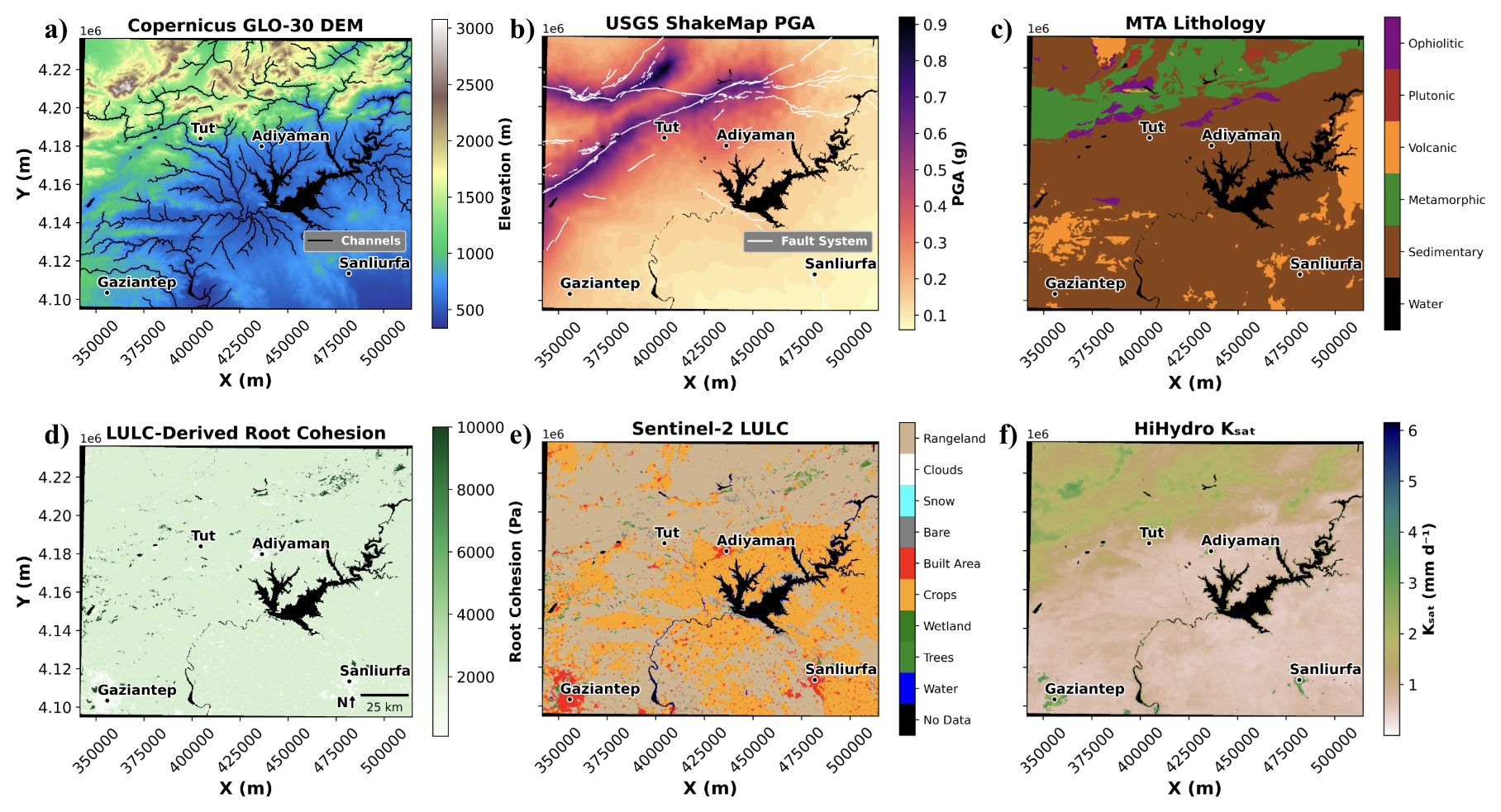
Figure 3 Illustration of model-data integration of remote sensing products into Landlab as fields: (a) Copernicus GLO-30 DEM, (b) USGS ShakeMap PGA, (c) ESRI Sentinel-2 land use/land cover map, (d) root cohesion derived from LULC in panel (c) using literature derived values (Strauch et al., 2018), (e) MTA geologic map, and (f) HiHydro K_sat. All data are projected in WGS 84/UTM Zone 10N (EPSG:32610) for Landlab modeling. Copernicus GLO-30 DEM © ESA/Copernicus. ShakeMap PGA data © USGS. Sentinel-2 LULC map: ESRI|Powered by Esri; Sentinel-2 imagery © ESA/Copernicus. Geologic map © MTA. HiHydro K_sat data © FutureWater.

4.1 Land surface and soils data

We employed the Copernicus GLO-30 DEM for elevation, with values ranging from >3000 m in the northern mountain ranges to <500 m in the southern plains, over a distance of roughly 60 km. At high elevations (Z≥1200 m), 46 % of slopes exceed 15°, which is approximately the threshold slope for landsliding of saturated sand (Montgomery and Dietrich, 1994). We use Sentinel-2 Land Use Land Cover (LULC) to assign vegetation types and their associated root cohesion values as reported in Strauch et al. (2018; Fig. 3d and e), as well as plant functional type (tree, shrub, grass). Rangeland LULC, dominated by grass and shrub species, is prevalent in the upland region where landslides are observed. Herbaceous cover, such as grass and cultivated crops, dominates the lowland region. Root cohesion is primarily associated with rangeland and herbaceous cover, which generally exhibit a modal cohesive strength of 2–4 kPa, with small pockets of tree cover providing additional resistance.

We found that using only root cohesion values systematically overestimated landslide probability. To introduce cohesion and friction angle of hillslope materials, we use 1:500 000 geological vector maps of Türkiye (MTA, 2002) which characterize local rock lithology (Fig. 3c). Sedimentary and metamorphic cover dominates the geology of the study area. The lithologic map better delineates the landslide observations with change in rock type from metamorphic to sedimentary units compared to soil textural classes. Following Xi et al. (2024b), which present a comprehensive review of rock geotechnical parameters across various regions, we assign cohesion values of 14.4 kPa for sedimentary units (e.g., basin fill) and 38 kPa for metamorphic units (e.g., gneiss). As a result, total cohesion in the model is primarily influenced by contributions from rock strength. Incorporating rock-derived cohesion reduced the model bias and better reflected the mixed soil-rock conditions of the study area. As such with these parameters our model is suitable for landslides that erode the bedrock or triggered at the soil-bedrock interface, consistent with observations that a large proportion of failures in the study area originated as these types of failures (Görüm et al., 2023).

Soil thickness was defined using SoilGrids data for absolute depth to bedrock. We enhanced our soil thickness dataset for high-elevation areas by applying an elevation-dependent linear relationship in high-slope regions (>15 %), capturing the tendency for thinner soils in steep mountainous hillslopes due to reduced accumulation and increased erosion (Pelletier and Rasmussen, 2009). Applying these additional criteria provides soil thickness values in the 0.3–2.0 m range from low to high elevations. This range is consistent with the reported soil depths on steep mountainous hillslopes and is intended to avoid unrealistically thin or thick soil thickness values that could bias model stability predictions (Strauch et al., 2018). We note that this parameterization introduces uncertainty, as soil thickness can vary substantially due to local controls (e.g., lithology, vegetation) that are not resolved in this formulation. Leaf area index (LAI) used by the soil moisture model is obtained from NASA's MODIS (Moderate Resolution Imaging Spectroradiometer). Soil saturated hydraulic conductivity (K_sat), wilting point, field capacity, saturated water content (or porosity) and texture classifications were defined using the FutureWater HiHydro dataset. Following the observations of Assouline and Or (2006), gridded K_sat values were multiplied by 10 to account for anisotropy in lateral flow. This scaling reflects the tendency for lateral hydraulic conductivity to exceed vertical conductivity in soils, which enhances lateral downslope drainage and reduces local pore pressure buildup. A minimum value of 0.5 m d⁻¹ was imposed to avoid unrealistically low conductivity values that would otherwise promote excessive saturation leading to slope instability. These adjustments introduce uncertainty where site-specific constraints on hydraulic anisotropy are unknown. The soil textural distribution is characterized by two dominant types: medium soil texture in the uplands and fine soil texture in the lowlands, which correspond with the metamorphic and sedimentary lithologic types, respectively (Görüm et al., 2023). Upland versus lowland differentials in LULC and soil texture lead to differences in soil water parameters such as the saturated hydraulic conductivity (Fig. 3).

4.2 Model forcing data

Hydrological forcing is represented using daily-aggregated precipitation derived from the IMERG Version 7 product, which provides half-hourly global precipitation estimates. Daily-aggregated minimum (T_min) and maximum (T_max) temperatures across the domain were derived from ERA-5 temperature fields. PGA was retrieved from the USGS ShakeMap (USGS 2023a, b). PGA values are combined using the maximum values from the two major earthquakes to create a composite map of the strongest ground motion (Fig. 3). Cells at high elevations (Z≥1200 m) experienced an average PGA of 0.4 g, and up to 0.9 g adjacent to the fault system. The soil and water density terms in Eq. (1a) were assigned a constant value of 2000 and 1000 kg m⁻³, respectively (Pack et al., 2005). The factor of safety has been found to be largely unaffected to soil density (Hammond et al., 1992; Lepore et al., 2013).

4.3 Model experiments

We use a series of targeted experiments to explore how the landscape responds to compound seismic and climatic drivers. To address research question 1, the modeled hydrologic response to the 14–15 March AR event is presented first, with some reality-check against satellite-derived soil moisture (Sect. 5.1), followed by the corroboration of landslide hazard predictions for the same event using an inventory of observed coseismic and mapped rainfall-driven landslides (Sect. 5.2). We then compare probabilistic landslide hazard maps generated with and without earthquake legacy effects (Sect. 5.3), and explore how sequences of extreme seismic and rainfall events influence landslide hazards (Sect. 5.4), to address research question 2.

Finally, in Sect. 5.5, we develop a pre-event forecasting method for mapping post-seismic landslide hazards under the influence of earthquake legacy in advance of future extreme storm events. For this purpose, the IMERG data catalog is used to identify all rainfall events with return periods comparable to the 14–15 March AR (excluding that event). These rainfall data are used to generate a composite rainfall-driven post-seismic landslide hazard map, which is then compared with the actual landslide hazard map developed using the 14–15 March AR event. This approach provides a practical method for rapid mapping of post-seismic landslide hazards for disaster preparedness after large earthquakes. In all simulations mentioned above, the soil moisture model is run for a 7 d period for each selected rainfall event, by positioning the peak rainfall on day 5. This approach is used to represent the initial hydrologic conditions leading up to the peak rainfall and capture soil moisture decay after the rainfall. Models are run at a 90 m grid resolution to make a regional application computationally feasible. However, to incorporate the variability of local slopes in our probabilistic model, we used a 30 m DEM and estimated the parameters of a triangular distribution for slope within each 90 m grid scale. This method is preferred to retain distributed information on slopes, which is critical for landslide initiation in this regional application.

5 Results

5.1 Hydrologic response to 14–15 March 2023 AR

Modeled land surface hydrology for the study region, including spatial averages of model forcing and hydrologic fluxes during the 14–15 March AR event, is summarized in Fig. 4a and b. The spatial mean rainfall steadily increased from 13 March and peaked at just over 35 mm d⁻¹ on 14 March (Fig. 4a). In the days leading up to the AR, both the maximum air temperature and the difference between maximum and minimum temperatures decreased (Fig. 4a), reflecting the natural storm conditions (e.g., Dai et al., 1999). The convergence of these temperatures suggests increased cloud cover and cooler conditions, before the onset of rainfall on 12 March. Due to the southeast to northwest trajectory of the AR event and orographic lift (Görüm et al., 2025), the northeastern part of the domain experienced significantly higher cumulative rainfall than the average rainfall, with some IMERG cells reporting cumulative 7 d precipitation as high as 145 mm (Fig. 4c). Within the study domain, max peak daily rainfall observed by IMERG during the AR event was 104.6 mm d⁻¹, corresponding to an approximate 5-year return period estimated using Weibull exceedance probability applied to annual maxima of spatially maximum daily IMERG precipitation over the historical record (2000–2024; Fig. 8b). While IMERG slightly underestimates peak daily rainfall compared to rain gauge stations and ERA5 reanalysis at some locations, its spatial distribution aligns well with the observed AR core and areas with documented rainfall-induced impacts, such as Tut and Askerhan (Görüm et al., 2025).

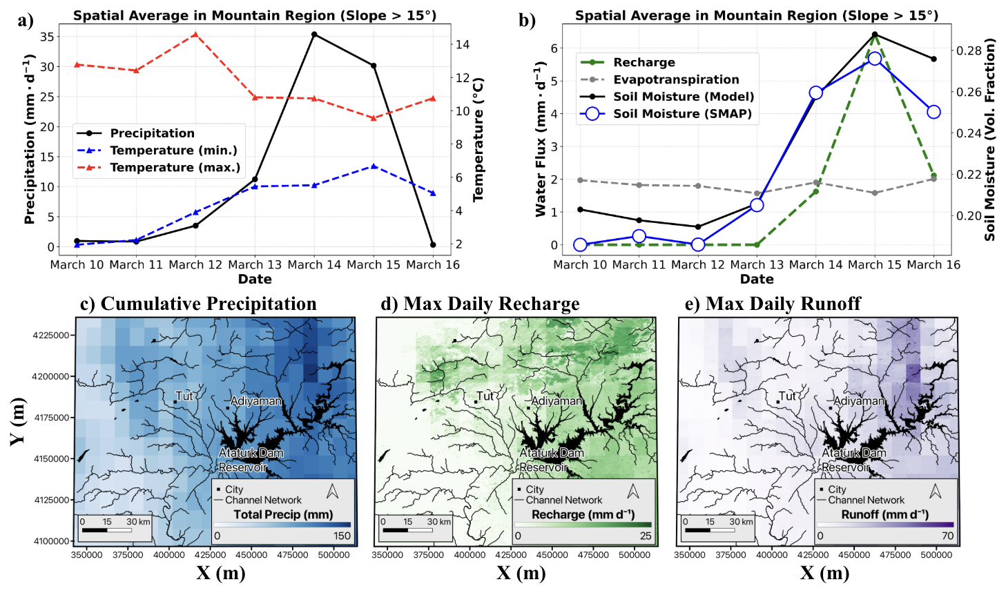
Figure 4 Landlab land surface model response to the 14–15 March AR event: (a) Spatial averages of meteorological forcing of 10–16 March including IMERG precipitation and ERA5 temperature time series. (b) Modeled local recharge, soil moisture, and evapotranspiration as well as SMAP L4 soil moisture observations. (c) Cumulative IMERG precipitation of the 7 d period, (d, e) modeled spatial maximum daily upslope average recharge (R) and local runoff (Q). Time series are spatial averages of the domain filtered for slopes >15° to report conditions in the mountainous regions. Max daily R and Q fields are Landlab outputs that are produced from combining the maximum values from the 7 daily response maps to create a composite map of the wettest conditions. All data are projected in WGS 84/UTM Zone 10N (EPSG:32610) for Landlab modeling. IMERG precipitation data © NASA. ERA-5 temperature data © ECMWF/Copernicus. SMAP-L4 soil moisture data © NASA.

We used soil moisture data from SMAP L-4 satellite derived-product to compare with the modeled soil moisture for the top 30 cm soil depth averaged over slopes > 15° (Fig. 4b). SMAP surface soil moisture estimates represent the vertical average of the top 5 cm of the soil layer. Both modeled and SMAP soil moisture show consistent values with each other especially during the storm, as they rise in tandem with rainfall to similar levels with a roughly 1 d lag. This lag in soil saturation may be due to factors like interception, infiltration and redistribution. Similar to soil moisture, a rise in recharge begins on 14 March at a small spatially averaged value (<2 mm d⁻¹) that grows to greater than 6 mm d⁻¹ on 15 March. This nonlinear growth suggests that the majority of the landscape that sustained heavy rainfall started to experience soil moisture levels above the field capacity, leading to sustained leakage from the conceptual root-zone of the model. Evapotranspiration (ET) losses trended around 2 mm d⁻¹, which is indicative of the cloudy spring-time conditions. Although this value is small, modeling ET is necessary to avoid overestimation of recharge, and allows more realistic closure to the root-zone water balance.

Composite maps of maximum daily rates, spanning the 7 d analysis period, report spatial average values of 13.3 and 5.7 mm d⁻¹ for local runoff and recharge, respectively. Over the 7 d analysis period, the average cumulative precipitation, runoff, and recharge were 82.0, 21.3 and 8.5 mm, respectively. This indicates that approximately 63 % of the total precipitation input was used to increase soil saturation and sustain ET. Notably, the average recharge over the entire domain is smaller than the recharge observed in the mountainous region (Fig. 4b), as lower elevations did not receive as much rainfall, where soils had lower K_sat and porosity. R rates reached up to 27.3 mm d⁻¹ on 14 March 2023 and were generally concentrated in soils within the Tut and Askerhan-Çelikhan regions and northeastern mountains. Q rates were modeled to reach 69.1 mm d⁻¹ on 14 March, occurring near and upstream of the saturated Tut, Askerhan-Çelikhan region, and city of Adiyaman, which was observed to experience excess runoff and flash-flooding. Additionally, these conditions triggered landslides and debris flows through the reactivation of coseismic landslides. The R field (Fig. 4d) is used to represent the local mean values of a log-normal distribution assumed at each grid cell. Section 5.2–5.4 use this map as forcing in the Monte Carlo solutions (Eqs. 2 and 6).

5.2 Landslide hazard model confirmation for the 15 March AR event

Before we present the regional model, a brief model confirmation is developed for the 15 March AR event, using the receiver operating characteristic (ROC) curves (Fawcett, 2006) at the Askerhan validation site (Figs. 2 and 5a). Both legacy and non-legacy models achieve similar overall performance, with AUC values of 0.7 and 0.67, respectively, indicating comparable performance in distinguishing between landslide source cells and non-landslide cells. However, there is a large difference between the models in terms of how this skill is distributed across probability thresholds. The non-legacy model reaches its optimal performance (i.e., the probability threshold that maximizes the sum of precision and recall) at an unrealistically low threshold (P(F)=0.0004), indicating that landslide initiation is only captured with unrealistically low probabilities. This reflects a bias for underprediction in the no legacy model, where even observed source areas are assigned low failure probabilities.

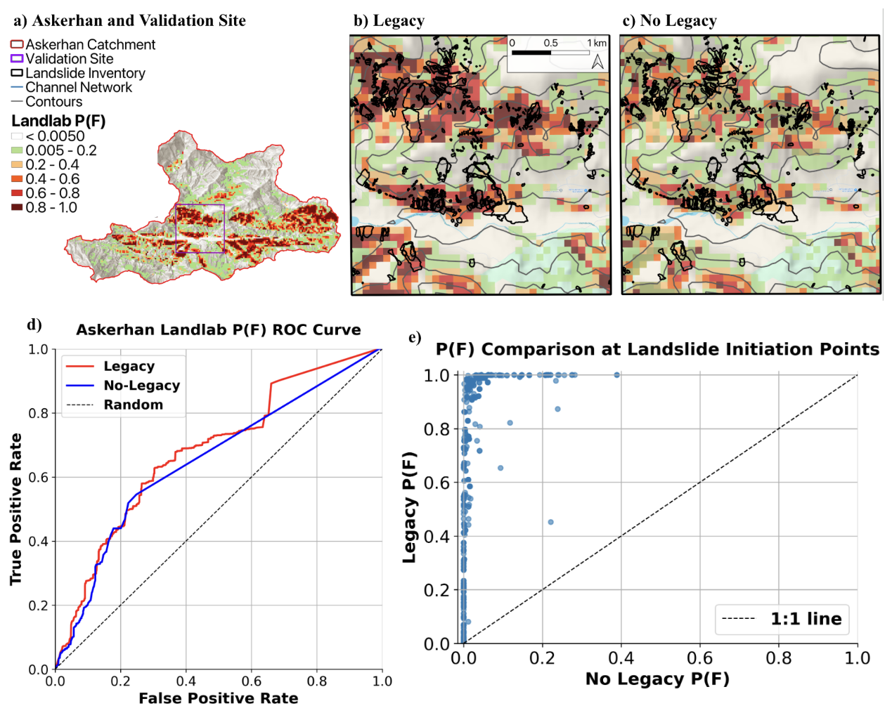
Figure 5 Comparison of model performance of legacy and non-legacy models within the validation site (a). Modeled P(F) at 90 m resolution, with subgrid parameterization for slope distribution: (b) with introduced earthquake legacy, (c) without legacy effects. Contours are at 100 m. (d) ROC curve based on the confusion matrix of the comparison between our observed landslide inventory source cells and modeled Landlab predictions at varying thresholds. Legacy and non-legacy scenario AUC values are observed to be 0.70 and 0.67, respectively. Source cells (observed samples) in the ROC curve analysis are the top 10 % elevation grid cells within the mapped landslide polygon. (e) One-to-one comparison of Landlab P(F) at landslide initiation points. Initiation points are the single highest elevation grid cell within the mapped landslide polygon.

In contrast, the legacy model achieves optimal performance at substantially higher and more physically meaningful thresholds (P(F)=0.3), indicating improved prediction of landslide hazard. This difference is further reflected in ROC behavior, where the non-legacy model exhibits an early plateau, reaching a maximum true positive rate (TPR) of 0.58 with false positive rate (FPR) of 0.25. The legacy model, however, continues to gain skill beyond this range, reaching TPR =0.91 at FPR =0.69 (Fig. 5d). This distinction is also evident in direct comparison of modeled P(F) at values at mapped landslide initiation polygons (Fig. 5e). The legacy model consistently assigns higher probabilities than the non-legacy model, with many source cells shifted above the 1:1 line. As a result, locations that are assigned low probabilities in the non-legacy case are elevated to moderate-to-high probabilities when legacy effects are included. This indicates that antecedent weakening improves the physical realism of predicted hazard, rather than simply increasing classification accuracy.

Qualitative comparison of spatial patterns supports this interpretation (Fig. 5b and c). The legacy model more clearly delineates observed landslides at intermediate-to-high P(F) values, whereas the non-legacy model requires near-zero thresholds to highlight similar regions. In addition, although modeled unstable areas may extend beyond mapped landslides in the legacy model, this should not be interpreted strictly as overprediction. The absence of mapped failures does not preclude instability, particularly given detection limitations and the potential for future failure under similar conditions despite appearing stable at the time of the inventory (e.g., Sidle and Ochiai, 2006; Baum et al., 2010; Borga et al., 2002). Instead, these areas can highlight sites for further investigation of missed landslides or impending failures, including terrain that may be potentially unstable when exposed to storms of similar magnitude to the March 2023 AR event.

5.3 Regional landslide hazards of the 14–15 March Atmospheric River

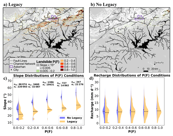
Earthquake legacy effects substantially increase the extent and magnitude of modelled landslide hazard for the 14–15 March AR event at the regional scale (Fig. 6). Using the legacy parameterization adapted from Xi et al. (2024a, b) (Eq. 3), total cohesion loss ranges from 52.2 % (PGA =0.15) to 67 % (PGA =0.75) relative to pre-seismic values. Overall, incorporating legacy effects increases the number of cells with (P(F)>0) by 329 %. The legacy model predicts (P(F)>0) across ∼41 % of the model domain, compared with only 9.6 % in the no-legacy model. To compare the two models, we use P(F)=0.3, the optimal threshold identified for the legacy model (Sect. 5.2), as the criterion for delineating high-hazard areas within the model domain (slope >15°). Without legacy effects, only 0.5 % of the landscape exhibits high-hazard potential during this AR event, largely confined to steep slopes (median 40°) (Fig. 6b and c). Such a limited landslide response, particularly concentrated in steep areas with thin soils that experience chronic instability, is expected from a storm with ∼5-year return period. However, when earthquake legacy is introduced, roughly 10 % of the landscape exhibits high-hazard potential (Fig. 6a and c), largely concentrated along the ruptured fault line from Tut to Askerhan and the badlands in the northeastern corner of the study area.

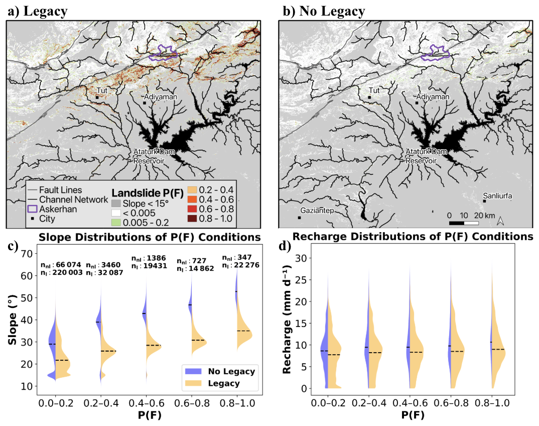
Figure 6 Landslide probability of failure P(F) maps for the central earthquake-impacted area overlain with mapped channel network for slopes greater than 15°: (a) with PGA-dependent legacy effect (Eq. 2) and (b) without legacy effects. (c, d) Comparison of (a) and (b) using violin plots of local slopes and daily R, respectively, for different bins of landslide probabilities, excluding areas of P(F)=0. For each probability bin, the number of grid cells classified as legacy (n_l) and non-legacy (n_nl) is indicated in the figure, horizontal dashed lines indicate the median value.

To further compare the two models, we examined slope distributions of potentially unstable cells across landslide probability bins (Fig. 6c). In every P(F) bin, the legacy model contains substantially more cells and lower median slope values than the no-legacy model, indicating that earthquake legacy lowers the critical slope required for landslide initiation. This effect becomes more pronounced at higher probability levels, with difference in median slopes growing from ∼10 up to 17.8° as P(F) increases. Across all plotted bins, the average reduction in median slope is 13.3°, showing a consistent shift toward failure on gentler slopes under legacy conditions. The increasing proportion of legacy-model cells in higher P(F) bins further indicates that earthquake legacy systematically shifts the landscape toward greater instability.

Across bins where P(F)>0.2, the median R required for potential failure in the legacy condition is an average of 1.2 mm d⁻¹ lower than in the non-legacy scenario. This indicates that while earthquake legacy does slightly reduce the recharge threshold for landsliding, the effect is not as pronounced as the ∼13° reduction in critical slope. This subtle difference can be due to a more uniform distribution of recharge rates across the landscape within the swath of the AR event. The contribution of recharge would have been more pronounced on the critical recharge rate solved for a given slope.

5.4 Landslide hazards under compound drivers

Existing landslide hazard assessment tools designed for global applications typically focus on seismic and rainfall drivers separately. In this section, we examine how landslide hazards change when these drivers are analyzed separately and in combination. Additionally, we compare these coseismic results to landslide hazards predicted for the 14–15 March AR event with post-seismic legacy conditions (Fig. 6a).

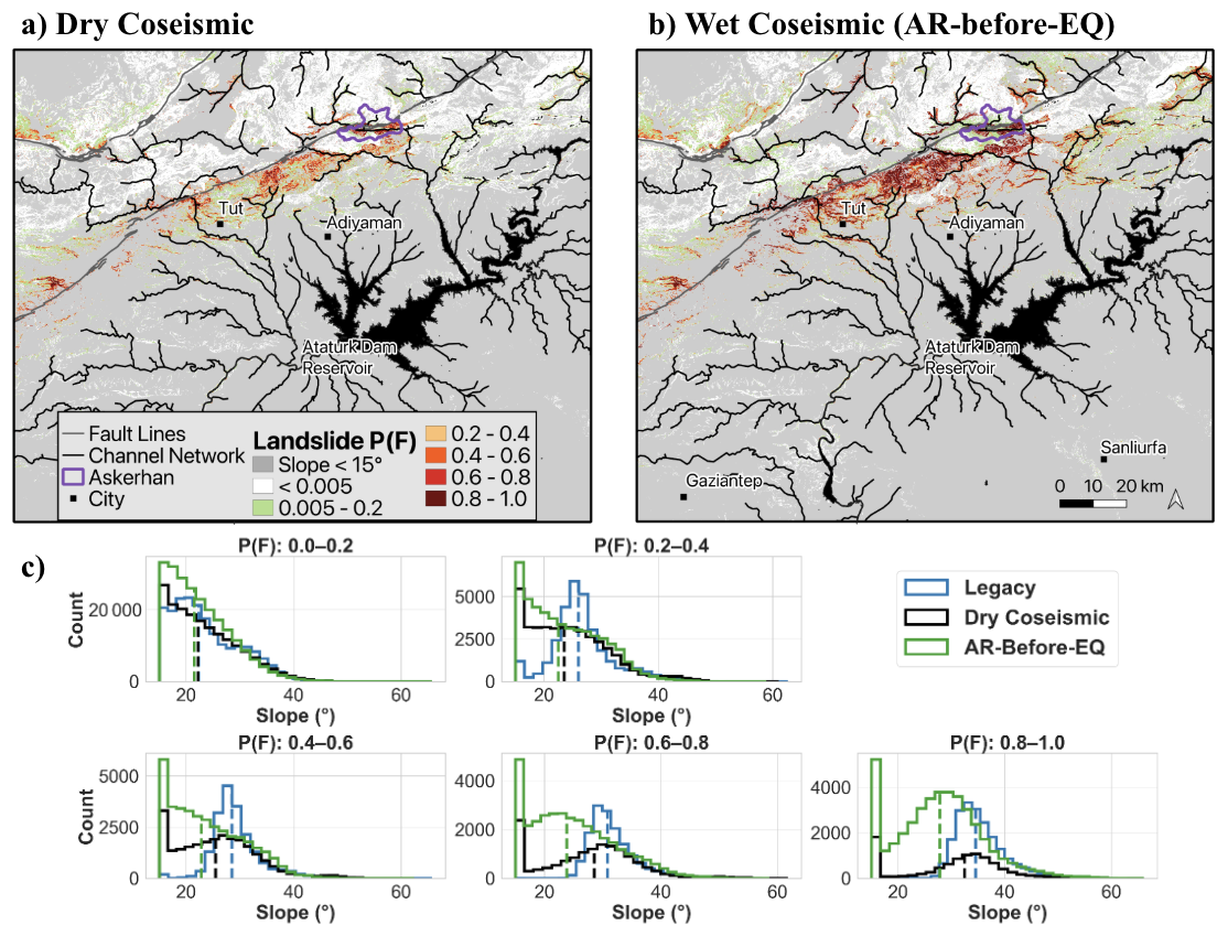
Figure 7 Landslide probability of failure P(F) maps for the central earthquake impacted area overlain with mapped channel network for: (a) dry coseismic scenario (no recharge) and (b) wet coseismic scenario, using recharge from the 15 March AR event. (c) Comparison of slope histograms (a, b), and the legacy model (Fig. 6a) across P(F) bins, excluding cells with P(F)=0.

Here two additional coseismic landslide model runs with seismic drivers acting on (a) dry soils, which provide some baseline landslide response of the landscape to seismic activity without any pore-pressure influence (Fig. 7a); and (b) wet soils, which use recharge conditions for the 14–15 March AR event are presented (Fig. 7b). The latter simulation illustrates the influence of extreme rainfall on amplifying the coseismic landslide hazard. These runs use P(F) from Eq. (6). Slope distributions for each scenario for different P(F) bins are shown in Fig. 7c.

Although there may be some control of soil saturation on landslide initiation during the 6 February 2023 seismic activity, here we evaluate model performance under dry soil conditions to establish a baseline for coseismic hazard prediction across the whole study domain. Using the mapped landslide inventory from Görüm et al. (2023), we compare modeled probability of failure to landslide locations aggregated at the 90 m model resolution. Because multiple landslides can occur within a single grid cell, this results in a reduced sample of 439 unique landslide cells, despite the inventory containing 2385 mapped landslides. This aggregation represents a limitation of the validation, as it reduces the effective sample size and may obscure finer-grid resolution variability in landslide initiation. Our non-landslide samples are randomly chosen outside the debris avalanche footprints and equal to the amount of grid cells containing landslide polygons (Strauch et al., 2018). The dry soil coseismic model yields an AUC of 0.83. This version of the model captures a substantial portion of the coseismic landslide signal with low false positive rates, supporting its use as a baseline for evaluating the compounding influence of legacy and hydrologic effects. However, its accuracy could likely be improved by incorporating realistic late-winter soil saturation levels typical of the region.

Interestingly, in all model simulations the low hazard bin (P(F)≤0.2) shows broadly similar slope distributions and median slope values (Fig. 7c). These low-hazard areas are concentrated mainly between the M_w 7.5 and 7.8 fault ruptures, where landslide initiation is limited across model scenarios, likely reflecting comparatively moderate ground shaking and the presence of stronger rock types such as metamorphic, plutonic, and volcanic units. At higher landslide hazard levels (P(F)>0.6), however, the number of cells within the probability bins increases in the order: dry coseismic < legacy < wet coseismic (AR-before-EQ). This pattern indicates that under saturated conditions, strong ground shaking from the earthquakes produces the largest landslide response, exceeding that produced by post-seismic legacy effects alone.

At P(F)>0.6 (high-hazard bins), both dry coseismic and wet coseismic scenarios show bimodal slope distributions with a low and an intermediate slope peak, whereas the legacy model is unimodal. The low-slope peak is more pronounced in the wet coseismic scenario, indicating that AR-driven recharge lowers the slope threshold for coseismic failure and expands hazard onto gentler terrain. The presence of a smaller low-slope peak even in the dry coseismic model confirms that PGA alone can promote failure on relatively gentle slopes. Across the high-hazard bins, median slopes in the wet coseismic case are about 7° lower than in the dry coseismic model, reinforcing the importance of antecedent wetness in amplifying coseismic hazard. In contrast, the legacy scenario displays a single dominant peak in the slope distribution with its median value increasing at higher P(F) bins. This unimodal behavior implies slope is a more direct control on P(F), potentially due to widespread cohesion weakening that reduces the failure threshold on already steep terrain, without generating a strong landslide response in low-slope areas.

Comparing the dry coseismic and legacy models helps identify locations for compound landslide hazards. For P(F) > 0.2, the dry coseismic model predicts median slopes that are about 3° lower than those of the legacy model and includes a low-slope peak (discussed above), but it contains fewer cells on slopes > 20°. This indicates that AR-driven recharge acting on seismically weakened hillslopes primarily expands the hazardous area over the slope ranges already impacted coseismically. The greatest post-seismic hazard remains focused on moderate-to-steep slopes (> 20°), but over a greater area extent than impacted by the coseismic model, whereas lower slopes (< 20°) remain comparatively less hazardous (Fig. 7c).

5.5 Post-seismic landslide hazard forecasting from satellite records of extreme events

In this section, we address the third research question posed in the introduction by combining historical extreme rainfall events with earthquake legacy effects to delineate future post-seismic rainfall-driven landslide hazards. Weibull exceedance probability is used over the IMERG catalog, which provided daily rainfall from 1 June 2000–31 March 2024, to determine the return period of annual maximum rainfall over the study domain (Makkonen, 2006; Fig. 8a). Extreme events in this region are often more spatially localized due to AR processes (Görüm et al., 2025). To detect the annual maximum rainfall in the historical data, we used a time series of spatial maxima of daily IMERG rainfall across the domain, as opposed to using spatially averaged daily rainfall.

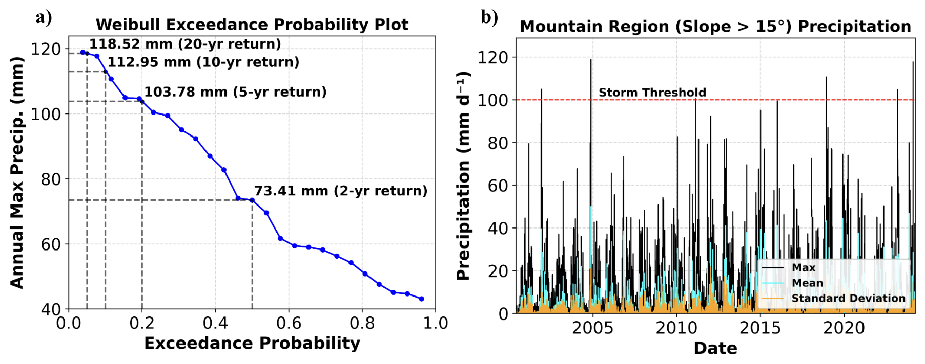
Figure 8 (a) Weibull exceedance probability plot fcor estimating return periods of extreme rainfall typical to the study domain. Standard Weibull plotting formula $P=\frac{m}{N+\mathrm{1}}$ is used to determine plotting position, where m and N correspond to rank order and sample size, respectively. (b) The IMERG version 7 rainfall time series used in (a) shows the average, maximum, and standard deviation of precipitation within the study domain. IMERG precipitation data © NASA.

We apply a threshold of 100 mm of daily rainfall as an indicator of an extreme event based on the 5-year return period level of rainfall (Fig. 8b). Four historical extreme precipitation events, excluding the 14–15 March 2023 event, are identified. The soil moisture model is run for each event for the 7 d window described in Sect. 3.4. Examples of the varying spatial distribution of cumulative 7 d rainfall and the composite max R field, representing the largest local upslope-averaged recharge from the historical extreme events are shown in Fig. 9.

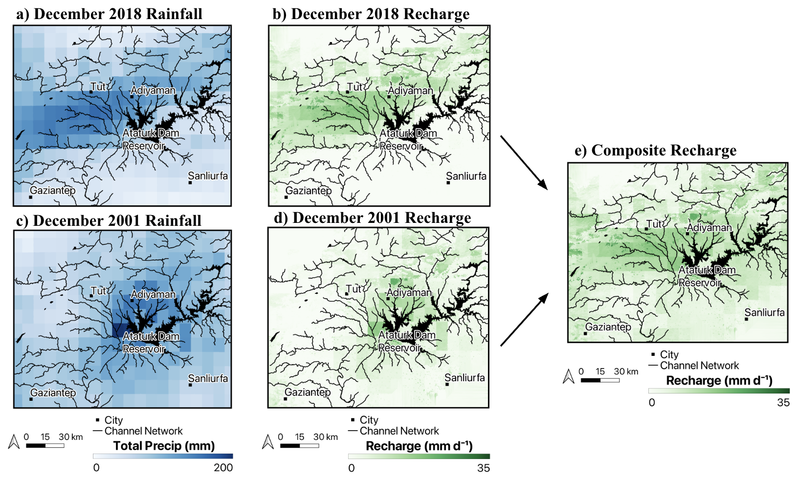
Figure 9 Cumulative rainfall and composited local maximum upslope average recharge for: (a, b) December 2018 and (c, d) December 2001 rainfall events; and (e) the composite recharge rate field of the combined pre-March 2023 extreme events identified in the IMERG catalog. Max daily recharge rate fields are derived from reduction processes outlined in Sect. 3.2 and are representative of the maximum daily recharge observed over the 7 d period for each cell. IMERG precipitation data © NASA.

To create a historical maximum R field, we combine the max R fields from the four extreme precipitation events by selecting the highest daily recharge rate for each cell across all events. This composite map highlights areas with higher recharge and saturation levels during extreme rainfall. Both the event-specific (Fig. 4e) and historical rainfall-driven (Fig. 9e) recharge rate fields show recharge concentrated in the Tut and Askerhan-Çelikhan region, the Burmapinar watershed and adjacent area north of the Ataturk Dam Reservoir, as well as the northeastern badlands. Notably, the historical recharge field has a higher spatial mean (6.7 versus 5.7 mm d⁻¹) and a higher spatial maxima (32.8 versus 26.7 mm d⁻¹) than the 14–15 March AR event.

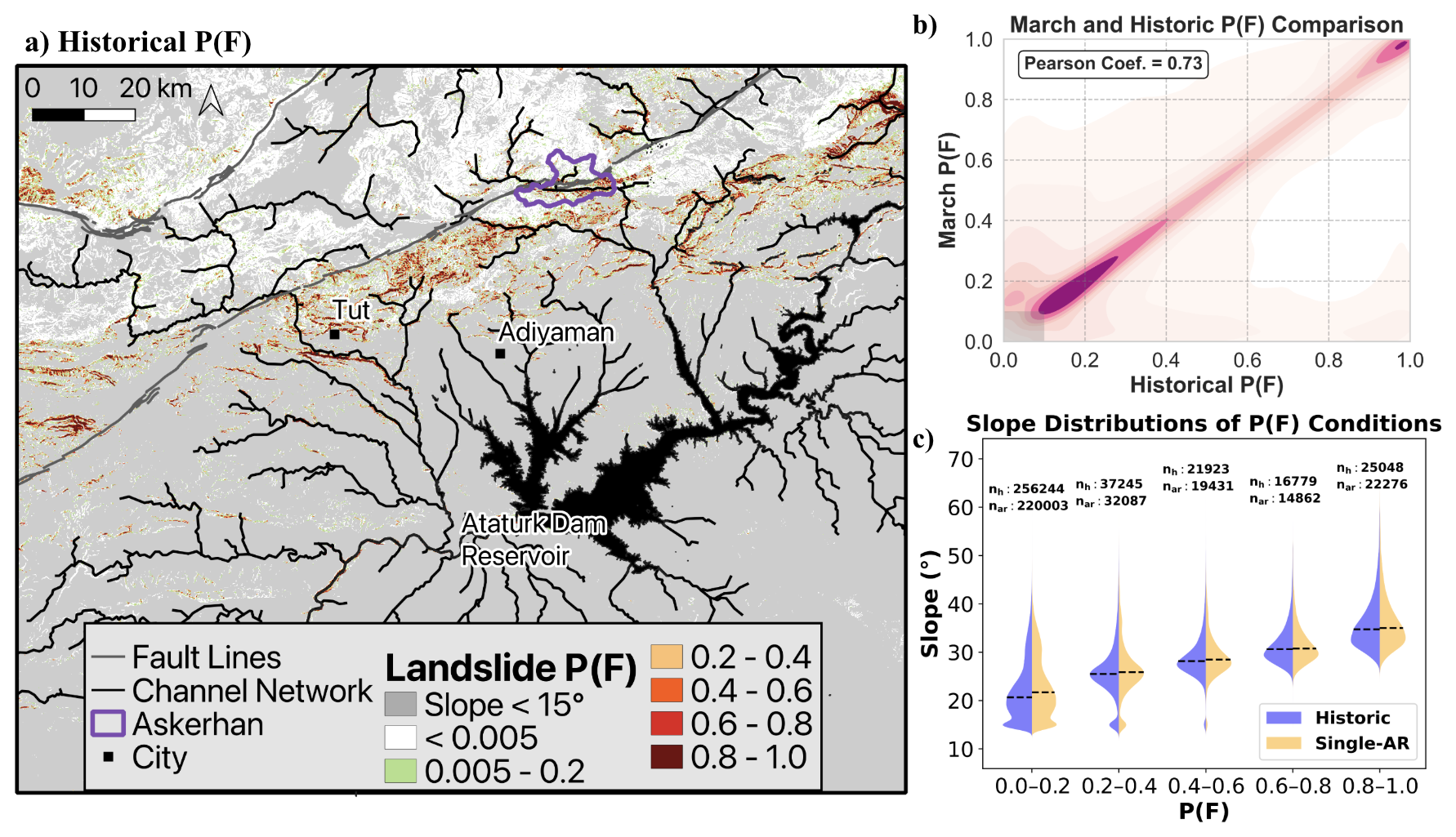
Figure 10 (a) P(F) map for the central earthquake-impacted area overlain with mapped channel network for simulations with PGA-dependent legacy effect (Eq. 6) and historical IMERG data driving the local recharge. (b) Kernel density estimation of March 2023 and historical model P(F), which visualizes the one-to-one cell comparison between the two models P(F) predictions. This comparison excludes generally stable cells (P(F)<0.1 in both models) to highlight point cloud density at areas where we may realistically see landsliding. These omitted cells are represented by the gray box. Cells with legacy P(F)<0.005 were excluded to evaluate how well the historic model reproduces areas of elevated hazard in the legacy scenario. (c) Comparison of March 2023 and historical rainfall-driven model using violin plots of local slopes for different bins of P(F). For each probability bin in panel (c), the number of grid cells classified as historic data based (n_h) and single-AR based (n_ar) is indicated in the figure. IMERG precipitation data © NASA.

The historical P(F) obtained using the compound recharge map aligns well with the P(F) of the 14–15 March 2023 AR event (Fig. 10a). Both models highlight hazards in areas prone to landsliding (Figs. 6a and 10a), such as high drainage zones and steep barren slopes, particularly in the Burmapinar watershed and the town of Tut which saw catastrophic damage (Görüm et al., 2023). To compare the consistency of the historical and single-AR scenarios at the cell level, we compare the prediction point cloud density using a kernel density estimation (Fig. 10b). Since landsliding is a rare occurrence that is spatially limited in a large region, we apply a 15° slope filter and a low probability threshold (P(F)≤0.2) to exclude areas where landsliding risk is low. This comparison reveals a strong one-to-one correlation between the two models at the grid-cell level (Pearson Coefficient =0.73), further confirming that the two methods identify high-risk areas at similar spatial proportions and locations. This agreement is reinforced by the slope distributions within each P(F) bin (Fig. 10c): violin plots show nearly identical distributions between the historical and single-AR scenarios, with median critical slopes varying by no more than 0.4°, suggesting the models converge on similar thresholds for failure across the landscape.

6 Discussion

6.1 Towards rapidly deployable landslide hazard models in seismic regions

Developing rapidly deployable regional models for co-seismic and post-seismic landslide hazards is critical because major earthquakes commonly impact large areas of mountainous terrain and cause extensive cascading downstream hazards (Fan et al., 2019; Tanyaş et al., 2017). In this paper, we identify two critical attributes of such regional models. First, in many post-earthquake settings, local observations are initially sparse, requiring model deployment to rely largely on global gridded land-surface, hydrologic, and meteorological datasets while being adaptable to use field observations collected in the aftermath of earthquakes and storms. Second, with increasing extreme precipitation events, including rapid dry-wet transitions (climate whiplash), across many tectonically active regions (Wang et al., 2023), models must produce probabilities that are physically meaningful to support early warning, emergency response, and mitigation planning. To advance such models, in this study we developed a parsimonious regional framework that integrates seismic and rainfall drivers with earthquake legacy effects.

Landslide hazard models are generally developed for rainfall (Baum et al., 2010; Strauch et al., 2018; Alvarado-Franco et al., 2017) and seismic (Jibson, 1993; Zang et al., 2020) drivers separately. This approach was arguably justified by model developers, as the underlying drivers and mechanisms are different and independent, and the likelihood of extreme seismic and storm events coinciding with each other is relatively low. However, critical-zone observations show that soil water, especially subsurface flow, often has a long residence time, interacts with groundwater, and is strongly linked to seasonal snow accumulation and melt dynamics (e.g., Montgomery et al., 1997; Anderson et al., 1997; Moon et al., 2026). This implies that unless earthquakes occur during the dry season, seismic shaking will usually coincide with some degree of soil wetness. Although this has been recognized in geotechnical research, particularly in liquefaction models for earthquake-induced ground failure (e.g., Baise et al., 2006), it is largely overlooked in coseismic models.

Regional models for coseismic landslide hazard mapping remain largely decoupled from hydrology. Data-driven models have only begun to incorporate simple hydrologic proxies, such as antecedent precipitation and topographic wetness index, and generally not at operational scales (e.g. Allstadt et al., 2022). More mechanistic models based on Newmark sliding block methods often neglect soil water altogether or impose spatially uniform assumptions for the relative wetness parameter, R_w (Eq. 1), across the landscape, to develop alternative hazard scenarios (Shao and Xu, 2022; Li et al., 2022; Djukem et al., 2024). However, these scenarios do not represent the space–time dynamics of watershed wetting and drying in relation to topography, radiative forcing and the many surface and subsurface controls documented in the hydrologic literature (e.g., Hartmann and Blume, 2024).

Earthquake legacy effects are an important preconditioning factor that is largely absent from post-seismic, rainfall-driven landslide hazard mapping. Much of the earthquake-legacy literature has focused on documenting the increase and subsequent decay of post-seismic landslide activity toward background rates through repeated mapping of new landslides and associated site characteristics (e.g., He et al., 2024; Tanyaş et al., 2021b, a). Models only recently began to represent legacy effects on landslide hazards, mainly in detailed process-based or hydromechanical models that require substantial data and site-specific parameterization, or through empirical inference of hillslope shear-strength reduction as a function of PGA from coseismic landslide inventories (e.g., Leshchinsky et al., 2021; Xi et al., 2024a, b). These approaches have improved understanding of post-seismic weakening, but to our knowledge, no modeling study has yet parameterized earthquake legacy for forecasting landslide hazards. We addressed this gap by including a simple PGA-linked legacy parameterization in our regional probabilistic framework, along with spatially distributed hydrologic forcing. The outcome of this model was reduction in critical slope for landslide probability classes. This implicitly represents the physical effect of seismic weakening on hillslopes, where shaking reduces slope shear strength through degradation of cohesion in soil and rock due to microfracturing, cracking, and regolith loosening, lowering the factor of safety threshold for failure and allowing previously stable slopes to fail at shallower angles (Brain et al., 2017; Keefer, 1984). This pronounced effect suggests that pre-seismic hazard maps likely underestimate post-earthquake risk under identical rainfall forcing, highlighting the need to update hazard analysis following major seismic events.

6.2 Towards realistic landslide probability forecasts

Hydrometeorological conditions before and after the 6 February 2023 Türkiye–Syria earthquake illustrate the need for using better hydrologic models for landslide hazards. Before the earthquake the region experienced a cold front that brought snowfall for 3 d before the earthquake. Air temperatures after the earthquake began to rise by late February, reaching above ∼10 °C at some locations. This warming trend caused snowmelt and elevated soil moisture in the mountains shortly before the arrival of the AR event on the night of 14 March. At the same time, strong shaking likely reduced hillslope shear strength by roughly 52 %–77 % in some areas (e.g., Xi et al., 2024a, b). When intense rainfall fell on these seismically weakened slopes, coseismic deposits were reactivated and widespread debris flows were triggered (Görüm et al., 2025).

Although the hydrologic representation developed here is imperfect, it is a step toward improving the hydrologic basis of regional landslide prediction. The single-layer distributed soil-moisture model supplies recharge to a steady-state kinematic-wave approximation of subsurface flow. Using gridded rainfall, temperature, and solar-radiation inputs, our parsimonious framework incorporates soil-moisture memory and spatial variation in vegetation and topography, arguably yielding a more realistic characterization of pore-water pressure than the fixed water-table assumptions commonly used in regional landslide hazard applications. When forced with historical gridded extreme events, such as ARs, each represented by a time window sufficient to capture soil water drainage, our framework provides landslide hazard forecasts with probabilities that we interpret as more realistic, especially when earthquake legacy events are included (Figs. 5, 6 and 11).

Model performance is commonly evaluated by how well hazard maps separate landslide from non-landslide cells across a range of thresholds, rather than by how realistic or “actionable” the predicted probabilities are for emergency response and hazard mitigation planning (Reichenbach et al., 2018). Here, we use “realistic” probabilities to mean probability levels that are physically consistent with observed failures and sufficiently interpretable for operational use, rather than probabilities that only preserve relative ranking. Our results show that incorporating earthquake legacy effects improves not only landslide delineation, but also the realism of the predicted probabilities. Although the no-legacy and legacy models have similar AUC values, 0.67 and 0.7 for mapping post-seismic landslides, the P(F) values at which these models reach optimal performance are significantly different, 0.0004 and 0.3, respectively. Figure 11 shows the modeled P(F) distribution across the domain and at mapped coseismic (90 %) and post-seismic (10 %) landslide locations. Although the landslide sample used in Fig. 11 is dominated by coseismic landslides, this comparison is informative because many of these scars were directly reactivated or destabilized during the 14–15 March AR event, making them relevant reference locations for evaluating post-seismic hazard (Görüm et al., 2025).

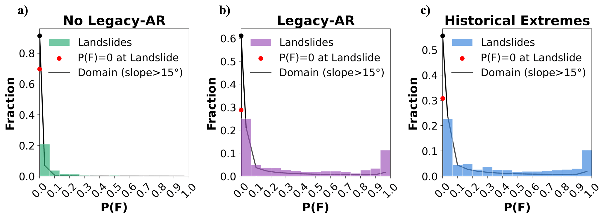
Figure 11 Distribution of modeled probability of failure, P(F), across the model domain for three post-seismic 14–15 March AR event scenarios (black lines), and distribution of P(F) at mapped landslide locations (colored bars): (a) without earthquake legacy; (b) with earthquake legacy; (c) earthquake legacy combined with historical extremes as forecast model. Large points at P(F)=0 indicate the fraction of the domain and mapped landslide locations predicted stable. The figure illustrates the shift from near-zero probabilities in the no-legacy case toward more realistic, moderate-to-high probabilities when earthquake legacy effects are included, and the similar probability structure reproduced by the historical-extremes model. Landslide data used is composed of 90 % coseismic and 10 % post-seismic landslides.

This distinction is evident in the probability distributions produced by the three post-seismic model scenarios (Fig. 11). In the no-legacy AR model, ∼94 % of the modeled domain and ∼68 % of observed landslides occupy cells with P(F)=0. This indicates that, although the model may retain some discriminatory skill, it tends to interpret that instability is highly unlikely around the coseismic landslide scars as well as at the newly identified post-seismic landslide locations. This result is physically plausible. Without earthquake legacy, we would not expect a regional rainfall event with an approximately 5-year return period to trigger widespread landsliding, and the concentration of elevated hazard within roughly 5 % of the steepest terrain is therefore reasonable (Fig. 11a). In contrast, the legacy-AR model shifts both the domain-wide probability distribution and the probabilities assigned to mapped landslides toward higher values: ∼60 % of the modeled domain and ∼30 % of observed landslides occupy cells with P(F)=0 (Fig. 11b). Roughly 10 % of the landscape and 30 % of the mapped landslide cells exceed the optimal probability threshold for high hazard (P(F)>0.3), while 15 % of the landscape falls in the very-high-hazard class (P(F)>0.8). The historical-extremes model shows a similar distribution to the legacy-AR case, indicating that the pre-event forecasting approach reproduces not only the spatial pattern of hazard, but also the broader probability structure. This suggests that historical extreme-event forcing can be used to anticipate not only where post-seismic hazard may occur, but also the magnitude of failure probability likely to accompany future extreme storms. However, these results should not be interpreted as a full calibration of absolute failure probability, but rather as evidence that including hydrologic response and earthquake legacy moves the model closer to an operationally meaningful probability framework.

6.3 Sequencing effects in compound seismic–rainfall landslide hazards

A key implication of this study is that compound landslide hazard in seismic regions should be viewed as a sequencing problem rather than simply as the addition of separate earthquake and rainfall triggers. Sequences may include seismic weakening followed by rainfall, seismic weakening followed by additional seismic shaking (aftershocks or doublets) and then rainfall, or rainfall followed by earthquake shaking. Rainfall following seismic activity has been widely documented in cascading earthquake hazard examples, including the Gorkha and Wenchuan earthquakes reviewed in the Introduction. The February 2023 Kahramanmaraş earthquake sequence, however, illustrates a more complex ordering of these drivers. The M_w 7.8 and M_w 7.5 events formed a doublet in which the second major shock, occurring nine hours later, likely triggered coseismic landslides on hillslopes already weakened by the first, and the 14–15 March AR then acted on this weakened landscape under seasonally wet late-winter conditions (Görüm et al., 2025). Our results show that these different sequences are not equivalent: rainfall before shaking primarily amplifies immediate coseismic instability, whereas rainfall after strong shaking acts on mechanically weakened slopes and sustains elevated hazard into the post-seismic period. The overlap we identify between dry coseismic hazard and post-seismic legacy-driven hazard further suggests that some terrain is exposed to repeated instability across the earthquake–storm sequence (Fig. 7).

The results presented here show that even a parsimonious framework can distinguish first-order differences between sequencing scenarios, including the larger hazard extent associated with AR-before-earthquake conditions and the broader post-seismic expansion of hazard under legacy weakening. In that sense, the framework is not intended to resolve the full mechanical complexity of repeated shaking and storm forcing, but it does provide a regional-scale way to identify where hydrologic preconditioning, repeated seismic loading, and post-seismic rainfall are most likely to interact. This is a useful step toward scaling sequence-aware landslide hazard modeling from data-rich research sites to earthquake response and recovery applications.

6.4 Beyond retrospective analysis: toward living landslide hazard models in seismic regions

Much of the current understanding of compound earthquake–rainfall landslide hazards comes from retrospective analysis of well-documented events. Such studies are essential for developing process understanding, identifying post-seismic weakening and reduced rainfall thresholds, and constraining the empirical and physical basis of hazard models. However, efforts to translate that understanding into forecast-oriented regional hazard assessment have been limited. Forecast-based regional systems do exist for rainfall-driven landslides, such as NASA's LHASA (Kirschbaum and Stanley, 2018), but these frameworks do not incorporate earthquake legacy effects or the interaction of seismic and hydrologic drivers. This is especially important in mountain belts where large earthquakes are expected but their timing is uncertain. The need is therefore shifting from explaining past landslide cascades to forecasting where, when, and under what combinations of drivers they are likely to occur.

A key challenge is that hazard in mountain regions depends on evolving landscape states, not only on the magnitude of a single storm or earthquake. Landslide response is conditioned by antecedent wetness, rainfall and snowmelt rates, sediment storage, vegetation disturbance, and prior topographic change. These controls can persist for years and may be reorganized by repeated earthquakes, storms, and hillslope and channel erosion. In this sense, landscape evolution is not just a long-term geomorphic background, but part of the hazard system itself. Regional forecasting frameworks therefore need some representation of longer-term environmental and geomorphic memory, including how past disturbances alter subsequent hydrologic and mechanical response. Earth-surface dynamics frameworks such as Landlab, used here for event-based hazard modeling, also provide a pathway for exploring these interactions over longer timescales, from decades to centuries (e.g., Campforts et al., 2020). The framework developed here is a step in that direction. It demonstrates features for modeling post-event observations, but also for prospective hazard assessment before future storms or earthquakes.

A useful long-term goal is the development of “living” regional hazard models that are established before disasters occur and then updated as new information becomes available from remote sensing, field observations, and evolving process understanding, consistent with emerging Digital Risk Twin concepts in disaster risk management (Ghaffarian, 2025). In seismic regions, this would mean establishing hazard frameworks in advance and driving them with historical climate and disturbance records to characterize system behavior and generate probabilistic scenarios of future compound hazards. These frameworks could then be refined with landslide inventories, field observations, remote sensing products, and new process understanding after major events. In this sense, the present framework can be viewed as an early step toward regional Digital Risk Twin–type approaches for landslide hazards in seismic regions, where forecasting, updating, and scenario testing are treated as part of the same hazard management problem. Natural next steps include extending the framework with landform evolution theory and more realistic hydrology to model cascading hazards through time, drawing on the growing number of post-event ground-based and satellite-derived datasets being collected in this earthquake-affected region.

7 Conclusion

Regional landslide hazard models have typically treated seismic and rainfall triggers separately. Compound drivers and earthquake legacy effects have mostly been examined in case-specific studies using data-intensive models with limited regional transferability. This paper bridges this gap by developing a rapidly deployable regional framework that integrates seismic and rainfall triggers with post-seismic legacy effects using global datasets.

Incorporating earthquake legacy effects substantially improves post-seismic hazard representation by shifting predicted failure out of unrealistically low probability ranges and into more physically meaningful and operationally useful probability classes, as well as provides moderate improvements to model prediction accuracy.

Sequencing of rainfall and seismic forcing shows that hydrologic preconditioning of extreme rainfall amplifies coseismic hazard, while post-seismic rainfall acts on mechanically weakened slopes to sustain elevated hazard during recovery.

Historical extreme rainfall records can be used to generate pre-event post-seismic hazard forecasts that closely reproduce the spatial pattern and probability structure of the March 2023 AR-driven hazard. The framework provides a practical basis for early warning, emergency response, and mitigation planning in seismic regions, and can be extended toward updateable “living” hazard models as new post-event data become available. Our approach also demonstrates the following points.

• Across the full study domain, the dry coseismic model yields a conservative performance that reflects dry antecedent conditions and provides a baseline for evaluating added effects of legacy and hydrologic forcing. Accuracy could likely be improved by calibrating soil saturation to February conditions typical to the area.

• Incorporating earthquake legacy effects leads to a ∼13° reduction in median critical slope for landslide initiation compared to the non-legacy model, indicating that slopes considered stable before an earthquake may become highly susceptible afterward. This suggests that pre-earthquake hazard maps may significantly underestimate post-earthquake risk, reinforcing the need to update hazard assessments following major seismic events.

• The scenario where the AR event precedes the earthquakes shows the greatest landslide hazard, pointing to a potentially important hazard scenario not seen in the historical record and highlights the need for more research on how the timing of storms and earthquakes influences landslide risk.

It should be noted that validating hazard maps remains uncertain, particularly in remote mountainous regions where landslide inventories are often incomplete. An additional and more comprehensive evaluation of model performance would benefit from further field investigations to identify landslides or signs of instability that may have been missed in our satellite and mapping derived inventory.