Climate change may increase landslide frequency despite generally drier conditions in the Mediterranean area

This study presents a methodological framework to investigate the impacts of climate change on rainfall-triggered landslides at the subregional scale. Focusing on a ∼170 km² area in the Partenio Mountains in southern Italy, we employed regional rainfall projections (CORDEX) under moderate (RCP4.5) and high (RCP8.5) emission scenarios for 2006–2070. Rainfall data were bias corrected with observations from 2006–2023 and benchmarked against a synthetic dataset generated through stochastic reproduction of currently observed conditions. Physically based simulations of hydrological processes, coupled with slope stability analyses that account for unsaturated soil conditions, enabled event-by-event identification of landslides throughout the period. Statistical comparisons between scenarios were conducted across three rainfall homogeneous subregions. Results show a general tendency toward drier soil conditions, consistent with regional-scale climate studies, but with increasing rainfall variability across subregions. Despite this drying trend, projections indicate a significant rise in landslide occurrence, with a faster increase under RCP4.5 when compared to RCP8.5. This counterintuitive outcome reflects shifts in rainfall dynamics: under RCP8.5, landslides are mainly linked to more intense triggering rainfall, while under RCP4.5 they result from a combination of wetter antecedent conditions and more intense early-peak rainfall events. These findings emphasize the critical role of antecedent soil moisture in landslide initiation by showing its stable influence on landslide occurrence despite the rapid evolution of climate change. Overall, the methodology provides a transferable framework to assess local climate change impacts on geohazards by integrating bias-corrected climate projections with physically based hydrological–geomechanical modeling.

1 Introduction

Understanding how the evolving climatic drivers regulate landslide occurrence is essential for adapting hazard management practices at local scales in landslide-prone regions, within a climate change context. Rainfall-triggered landslides are a complex natural hazard, resulting from non-linear interactions among meteorological forcing, transient subsurface hydrology, and the mechanical properties of slopes. Key triggering mechanisms are caused by infiltration of rainfall into the soil and even its interaction with underlying bedrock conditions, elevating pore water pressure, reducing effective stress, and weakening shear strength along potential failure planes. These mechanical responses are determined by rainfall characteristics (e.g., intensity, duration, accumulation) and strongly influenced by hydrological conditions, determining soil water content conditions, which are shaped by preceding hydrological processes. The “filling-storing-draining” concept offers a valuable framework for interpreting the temporal evolution of pore pressures, describing how slope materials sequentially absorb, retain, and discharge infiltrated water (Bogaard and Greco, 2016). Understanding these processes is essential for assessing slope stability under dynamic climatic conditions, influenced by atmospheric dynamics and climate change.

The influence of climate change on rainfall patterns is increasingly evident in observational records and consistently projected by climate models for the coming decades (Avino et al., 2024; Capozzi et al., 2023; Gründemann et al., 2022). Ensembles of high-resolution projections, such as those developed under initiatives like EURO-CORDEX, provide detailed insights into expected future climatic conditions, often indicating significant alterations in precipitation characteristics across Europe and other regions by the end of the 21st century (Jacob et al., 2014). However, raw outputs from Regional Climate Models (RCMs) often contain magnitude biases, leading to discrepancies in key statistical properties when compared to detailed observations in rain gauges. Since hydrological and slope stability models are sensitive to the magnitude and variability of meteorological inputs, bias correction is essential for reliable climate impact assessments on local and regional scales (Ehret et al., 2012; Teutschbein and Seibert, 2012). Parametric quantile matching (QM), as applied in the ISIMIP framework (Davie et al., 2013), adjusts simulated distributions to match observed ones using additive or multiplicative corrections, depending on the variable type. Advanced methods such as the Multivariate Recursive Nested Bias Correction (MRNBC) extend QM to preserve inter-variable correlations and temporal consistency (Kim et al., 2023). For capturing extremes, the Quantile Matching for Extremes (QME) method enhances resolution in distribution tails, essential for landslide-triggering rainfall (Vogel et al., 2023). By ensuring more realistic inputs, bias correction improves the representation of hydrological processes under climate change, particularly those influencing slope saturation and landslide occurrence (Peter et al., 2024).

Addressing the inherent complexities and uncertainties in predicting landslide occurrence, especially over local areas (i.e. between 10² and 10³ km²) under future conditions, necessitates innovative approaches. Physically based synthetic data generation has emerged as a powerful tool in this domain, enabling researchers to overcome limitations associated with sparse observational records and to explore slope responses across a wide spectrum of potential hydro-meteorological conditions (Roman Quintero et al., 2023, 2024a). By simulating extensive datasets, often employing stochastic models for rainfall (e.g., Peres and Cancelliere, 2014, 2016; Rodriguez-Iturbe et al., 1987a) coupled with hydrological and slope stability models, it becomes possible to systematically investigate the influence of various factors and estimate landslide probabilities under diverse conditions. This involves differentiating between the influence of relatively static landscape attributes (e.g., topography, soil type distribution, geology, land cover) and highly dynamic factors (e.g., rainfall forcing, evolving soil moisture fields) (Bozzolan et al., 2025; Fang et al., 2024). Such methodologies are particularly pertinent for assessing the potential impacts of climate change, as they allow for the explicit incorporation of altered dynamic drivers (e.g., modified rainfall inputs derived from climate projections) to evaluate consequent shifts in slope stability and landslide likelihood at local scales (Gariano and Guzzetti, 2016; Stoffel et al., 2014).

Despite extensive research on the effects of climate change on hydrometeorological hazards, the systemic understanding of how evolving climate conditions translate into changes in landslide occurrence remains limited, particularly at the subregional scale. Most existing studies rely on empirical correlations between rainfall trends and landslide records, demonstrating with data records the observed effects of climate change on this geohazards, but often overlooking the physically based processes that link climate forcing, subsurface hydrology, and slope stability (Crozier, 2010; Gariano et al., 2015; Semnani et al., 2025; Stoffel et al., 2014). In particular, there is a lack of systematic investigation into how projected changes in rainfall regimes, characterized by increased temporal variability and altered antecedent moisture conditions, may influence the triggering mechanisms of rainfall-induced landslides. Moreover, while ensemble climate projections are widely used to assess future climatic patterns, their large variability can obscure the understanding of how climate change affects highly non-linear processes such as slope response to precipitation; an aspect that has been rarely explored through process-based modeling frameworks (Buonacera et al., 2025; Crozier, 2010). Addressing this knowledge gap requires integrating bias-corrected regional climate projections with coupled hydrological–geomechanical simulations to evaluate how subsurface processes respond to changing climatic forcing and to quantify the potential for increased landslide occurrence despite any overall rainfall trend.

This study aims to propose a novel methodology to quantitatively assess the local impacts of regional climate change on rainfall-triggered landslide occurrence. The methodology, applied within a study area, uses a coupled physically based hydrological and slope stability modeling framework driven by bias-corrected RCM outputs under different emission scenarios, and incorporates current climate conditions for benchmarking. We analyze the complex interactions between future climate scenarios, local-scale hydrological responses, and slope stability dynamics. The core objective is to address two fundamental research questions regarding future landslide probability of occurrence in subregional scales: (1) How is rainfall expected to change in terms of event magnitude, duration and temporal distribution? And (2) How will those changes affect future landslide occurrence? The outcomes of this research are expected to provide insights into landslide probability quantification, susceptibility, hazard and landslide risk assessments under changing climate conditions.

2 Materials and methods

To reveal the impact of climate change on the occurrence of rainfall-triggered landslides, this study uses a physically based modelling framework. Figure 1 illustrates the conceptual framework linking climate forcing, hydrological processes, and slope stability assessment from a dynamic perspective. At the highest level, socio-economic development (SD) drives greenhouse gas emissions, represented by the Representative Concentration Pathways (RCs), which in turn influence global and regional climate conditions. These forcings affect temperature (T) and atmospheric dynamics (AD), which jointly control precipitation (P) regimes and evaporation–evapotranspiration (E–ET) processes.

Figure 1 Influence diagram displaying the methodological framework proposed in the study.

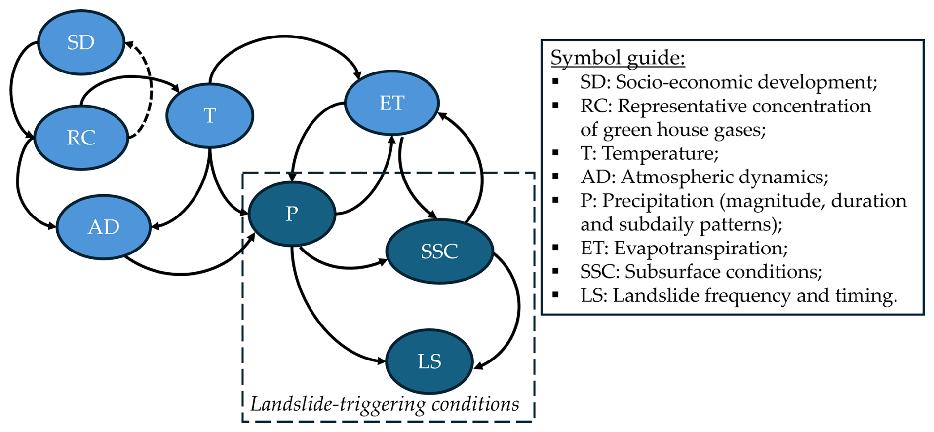
The meteorological forcing (P and ET) plays a central role, acting as the primary external driver of landslide-triggering conditions. Precipitation frequency, magnitude, duration, and sub-daily distribution determine the temporal evolution of subsurface conditions (SSC), such as soil moisture and pore water pressure. These conditions are critical in setting the proneness of a slope to failure. Simultaneously, ET regulates water loss from the soil–plant–atmosphere system, modulating SSC and influencing the balance between infiltration and drainage. Ultimately, landslide frequency and timing (LS) emerge as the response variable of this coupled system, reflecting the combined effects of precipitation forcing and antecedent subsurface conditions. Rainfall infiltration and slope stability were simulated with a physical based numerical model (see Sect. 2.2). While the bidirectional relationship between temperature (T) and evapotranspiration (ET) is fundamental to the surface energy balance, T is treated here as an external forcing to compute ET unidirectionally.

2.1 Study area

This study investigates a ∼ 170 km² landslide-prone area within the Partenio Massif, Campania Region, southern Italy (Fig. 2). Located in the southern Apennines, this geomorphologically homogeneous subregion is prone to shallow landslides and debris flows.

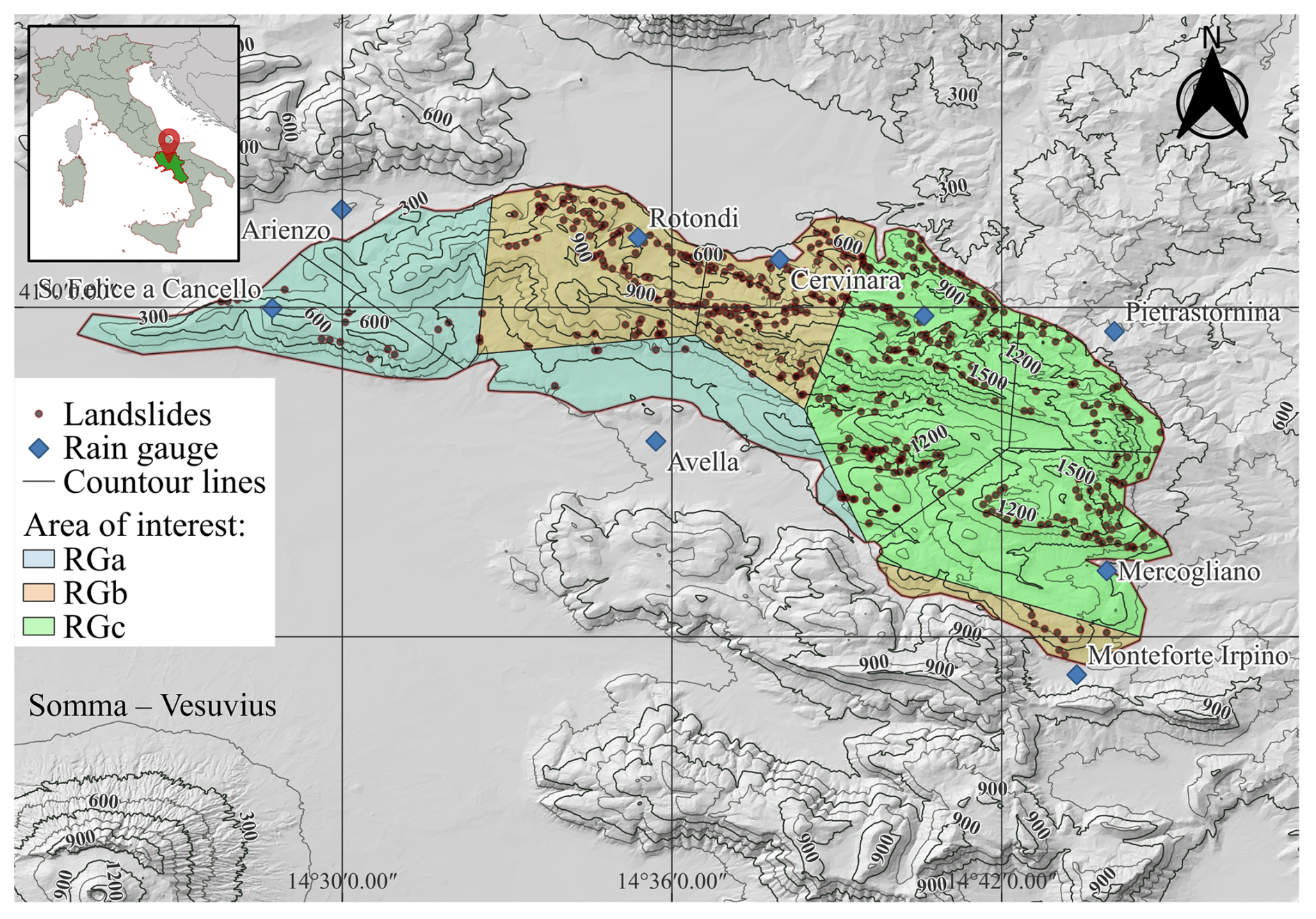
Figure 2 Landslide-prone area in the Partenio Mountains, Campania Region, southern Italy, and the three subregional groups RGa (blue), RGb (orange), and RGc (green), characterized by similar precipitation characteristics. Landslide data are taken from the Inventario dei Fenomeni Franosi d'Italia (Iadanza et al., 2021).

The area has a typical Mediterranean climate, with average annual precipitation ranging between 1000 and 2000 mm. Total potential evapotranspiration ranges from 700 to 800 mm (at 400–750 m a.s.l.), and mean daily temperatures vary from approximately −4.0 °C in the cold season to 30 °C in the warm season.

The area is monitored by a network of nine meteorological stations managed by the Italian Civil Protection Agency. These stations, operational since 2003–2004, are equipped with rain gauges providing observed sub daily rainfall data, which was used in the present study. The geographical representation, constructed with Voronoi polygons, represent areas where rainfall events are statistically similar.

The rainfall stations were categorized into three distinct sub-regional groups (RGa, RGb and RGc) based on both their spatial distribution and the statistical similarity of the rainfall events. Pairwise Kolmogorov–Smirnov (KS) tests were conducted at a 5 % significance level (α=0.05).

In fact, according to observed rainfall, mean annual rainfall increases from the least rainy group, RGa (∼ 1050 mm yr⁻¹), to the intermediate group, RGb (∼ 1600 mm yr⁻¹), and finally to the rainiest group, RGc (∼ 1820 mm yr⁻¹).

Geomorphologically, the Partenio Mountains feature steep slopes covered by a thin mantle of coarse-grained volcanic soils (pyroclastic deposits), ranging from less than 1 m on steep parts to over 6 m in flatter areas (Del Soldato et al., 2018; De Vita and Nappi, 2013). These soils overlie a fractured and karstic limestone bedrock. Due to their gentle airfall deposition, the soils have high porosities (up to 0.7), making them highly permeable in saturated conditions, yet they maintain a high shear strength with friction angles around 38° (Picarelli et al., 2006).

This combination of pyroclastic deposits and fractured limestone creates a hydrogeological setting contributing to rapid pore pressure responses. The uppermost highly weathered part of the limestone bedrock, known as epikarst (Celico et al., 2010; Williams, 2008), hosts a perched aquifer during wet seasons. This aquifer exchanges water with the unsaturated soil mantle, a process that becomes evident in mid-winter when several ephemeral springs feed local streams (Roman Quintero et al., 2023).

Previous investigations have shown that while the landslide-prone area is relatively uniform, landslide initiation is highly sensitive to specific rainfall thresholds and pre-existing soil wetness states. This highlights the importance of integrating both short-term rainfall events and long-term hydrological conditions in modeling frameworks (Marino et al., 2020a; Picarelli et al., 2006; Roman Quintero et al., 2025; Del Soldato et al., 2018; De Vita and Nappi, 2013).

2.2 Numerical Simulation of Hillslope Hydrological Processes and Stability Analysis

The hydrological processes governing the water storing in the sloping pyroclastic soil deposits, despite the rainfall itself, have been proved to be linked to the infiltration capacity of the soil (Greco et al., 2023; Roman Quintero et al., 2023). Figure 3 represents the main physical processes affecting the water balance of slopes in the area, including shallow surface processes as rainfall infiltration and evapotranspiration, and deeper ones as water leakage to the perched aquifer and drainage to deeper systems.

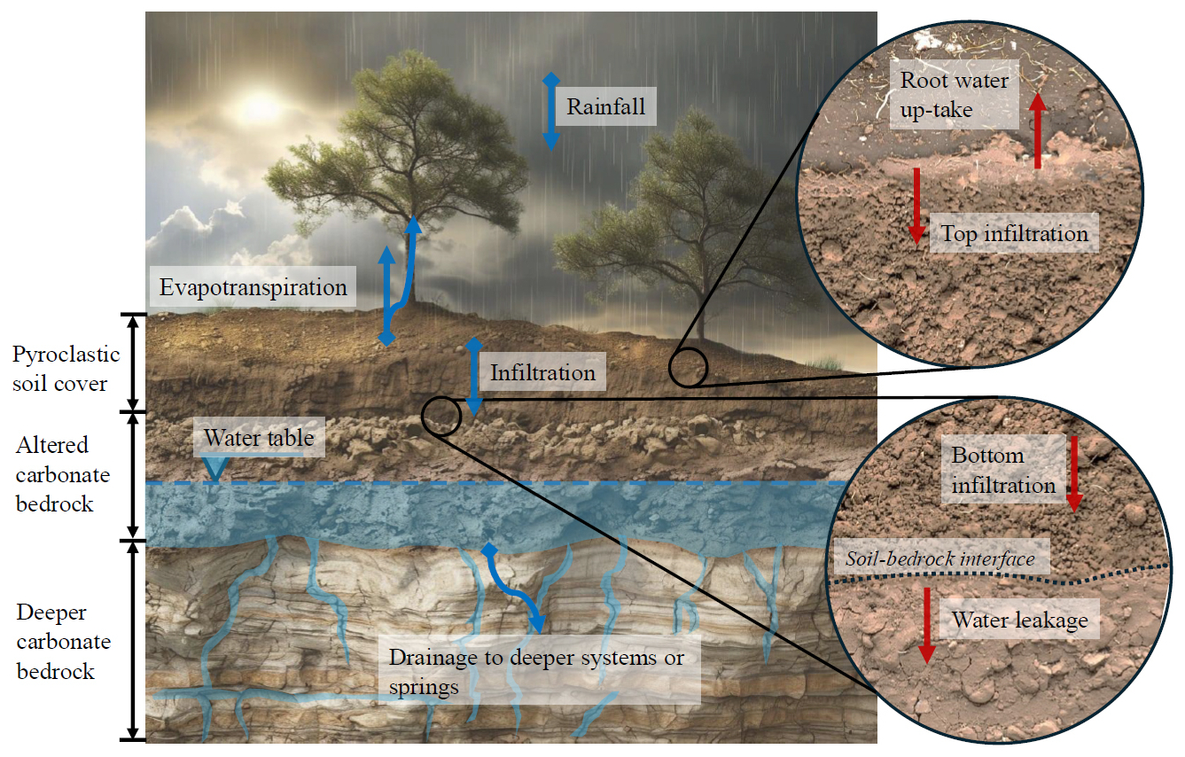
Figure 3 Main hydrological processes affecting the water cycle and water stored in the pyroclastic soil cover affecting slope stability in the landslide-prone study area.

A previously developed and validated physically based model incorporating dominant hydrological processes at the hillslope scale was implemented to characterize the transient water dynamics in landslide-prone slopes within the study area (Greco et al., 2013, 2018; Marino et al., 2021, 2020a; Roman Quintero, et al., 2024b). The modeling framework numerically solves the 1D Richards equation for unsaturated flow through the pyroclastic soil matrix, coupled with a bucket-type groundwater representation of the Epikarst aquifer, connected to the soil deposits through its lower boundary condition.

The pyroclastic soils of the area exhibit high porosity (θ∼ 0.65–0.7), resulting in saturated hydraulic conductivity values ranging between about 10⁴ and 10⁵ m s⁻¹. These hydraulic properties renders very unlikely the overland runoff generation, when compared with the observed maximum hourly rainfall intensities, always less than 70 mm h⁻¹, justifying its exclusion from the simulations (Picarelli et al., 2020; Roman Quintero et al., 2025).

Simulations were conducted by running the model across different rainfall time series. While the meteorological forcing imposed by rainfall will be explained in detail later, we used both time series representing climate change scenarios and current climate conditions. In turn, the potential evapotranspiration (PET) was assumed to variate on a monthly basis and was estimated with the Thornthwaite formula (Marino et al., 2020b).

For simplicity, under all projected conditions, PET was assumed to be equivalent to that of the observed period, ranging between 4–5 mm d⁻¹ in summer and less than 1 mm d⁻¹ in winter. This assumption is supported by two main reasons. First, although evapotranspiration influences soil moisture seasonally, its role in slope instability is likely minor because rainfall-triggered landslides typically occur during wet and cold periods when PET is only 0–2 mm d⁻¹ compared with the ∼ 300 mm over 2–3 d of triggering rainfall (Greco et al., 2021). Furthermore, while PET is projected to increase slightly (mainly in summer and only marginally in winter) its relevance for slope stability remains limited, especially because actual ET is constrained by soil-water availability and no major vegetation changes are expected that would enhance ET in proportion to PET.

Landslide-prone slopes associated with the most impactful landslides in the study area share similar geomorphological characteristics: a sandy size pyroclastic soil cover of approximately 2 m deep, where typically encounters a limestone bedrock, laying on slopes with inclinations of about 40° (Greco et al., 2021). These particular conditions were used to calculate the Factor of Safety (FS), considering them as a proxy simulating the slope stability of such representative landslide-prone slope classes. The FS was simulated in an hourly scale along with the hydrological simulations, considering the failure surface at 2 m depth and accounting for unsaturated material conditions. The detailed property values and further model details can be found in Roman Quintero et al. (2025).

In synthesis, the numerical simulations were applied to nine rainfall time series representative of the locations shown in Fig. 2.

2.3 Projected rainfall under current and climate change conditions

This study uses rainfall projections to define three data ensembles representing both current and climate change conditions. For the currently observed climate, the Neyman–Scott Rectangular Pulse (NSRP) stochastic rainfall model was used to generate nine synthetic hourly precipitation time series at each observation point (rain gauges), each spanning 65 years and based on observed data, resulting in a total of 81 time series. This ensemble, referred to here as CTRL, covers the simulated period from 2006 to 2070 and serves as the reference for comparison.

Specifically, The NSRP model conceptualizes rainfall as a sequence of storm clusters, each composed of rectangular pulse cells with randomly distributed start times (Rodriguez-Iturbe et al., 1987; Cowpertwait et al., 1996). In this way, the duration of each pulse represents the lifetime of a rain cell, while the pulse height corresponds to rainfall intensity. When multiple cells overlap in time, their intensities are cumulatively summed to determine the total precipitation rate. Calibration of the NSRP model for the study area has been presented in previous studies and was performed using the method of moments (Peres and Cancelliere, 2014; Roman Quintero et al., 2023).

Climate change rainfall projections were extracted from regional climate studies from two sources: the EURO-CORDEX initiative, produced by several multinational climate modeling centers, and the Very High Resolution Climate Projections for Italy (VHR-PRO_IT), produced by the Euro-Mediterranean Center on Climate Change (CMCC Foundation). In both cases, the climate projection simulations start from 2006, but the CORDEX has projected data until 2100 while the VHR-PRO_IT until 2070. The CORDEX initiative represents a set of experiments developed under an international framework involving 26 climate modeling centers worldwide, contributing 11 regional climate model simulations. The data used in this study correspond to downscaled CMIP5 global simulations (at ∼ 12.5 km horizontal resolution, with 3 h temporal resolution), incorporating Representative Concentration Pathways (RCPs) (Moss et al., 2010; Taylor et al., 2012; van Vuuren et al., 2011). RCPs are a set of scenarios that integrate greenhouse gas emissions, concentrations, and land-use trajectories with socio-economic developments. Here, two scenarios were analyzed: RCP4.5 (including mitigation measures) and RCP8.5 (very high emissions, often termed “business as usual”) (van Vuuren et al., 2011). A total of 8 ensemble members were used here for RCP4.5 and 8 for RCP8.5 scenarios.

The second source consists of the VHR-PRO_IT dataset, which provides an additional ensemble member produced with the COSMO-CLM model at ∼ 2.2 km horizontal resolution and hourly temporal resolution. This initiative largely follows the CORDEX framework (from data management to experimental design), making it suitable for inclusion in the analysis. Specifically, VHR-PRO_IT downscales an existing regional dataset for Italy (Italy8km-CM; Bucchignani et al., 2016), which itself downscales the global forcing from CMIP5 simulations from different RCP scenarios.

In summary, we used a total of 9 ensemble members for RCP4.5 and 9 for RCP8.5 climate change scenarios, resulting in 81 study units (time series) at the observation points (rain gauge locations). Temperature projections from the same scenarios were also displayed to illustrate the co-evolution of the studied variables with temperature rise, although they were not directly used in subsequent calculations. Rainfall data from both sources were further spatially downscaled and bias corrected. The selected temporal resolution was 3 h, constrained by the EURO-CORDEX dataset. Simulations of hillslope hydrological processes and slope stability were then performed from 2006 (the standard baseline year for climate change projections) to 2070, limited by data availability in the VHR-PRO_IT dataset.

2.3.1 Statistical Bias Correction of rainfall projections

Since this study focuses on a local area in Partenio mountains of southern Italy, and the studied process is affected by extreme rainfall, we applied the Quantile Matching for Extremes (QME) method to further downscale rainfall to the observation points (rain gauge locations), and bias-correct climate model projections against observed data. The method was applied with data recorded from the stations between 2006 and 2023.

QME is widely used in meteorological applications and is particularly well-suited for studies where extreme rainfall events are a key focus (Peter et al., 2024). The procedure utilized here is fundamentally based on bias-correction procedure proposed by Dowdy (2023), enhanced by adding a previous correction step matching the number of rainy cells of modeled rainfall data, with the observed values. For a detailed view of the algorithm, visit the repository accompanying this study (Roman Quintero, 2025).

Before applying QME, the model and observed rainfall data were scaled to make them directly comparable. This normalization step ensures that both datasets share a common reference range, accounting for the rain gauge resolution (0.2 mm) and the maximum observed or simulated rainfall values for each case.

The bias correction was then carried out quantile by quantile. First, we estimated the empirical cumulative distribution functions (CDFs) of both the observed and modeled rainfall data. Each modeled quantile was then matched to its corresponding observed quantile, using both forward and backward scans to minimize mismatches. The final bias-corrected value for each quantile was obtained by averaging the results from these two scans.

To better capture the behavior of extreme events (a key objective of this study) an additional correction was applied to the upper tail of the rainfall distribution (above the 95th percentile). For this step, we compared the mean rainfall values of the observed and modeled datasets in this extreme range and adjusted the modeled values accordingly. When the extreme-value correction produced a larger adjustment than the standard quantile matching, the extreme correction was retained.

Finally, the resulting bias-correction values were applied to the scaled model rainfall data, producing a dataset with magnitudes statistically consistent with local observations while preserving the distribution of extreme events.

The bias-corrected rainfall projections were aggregated into discrete rainfall events. An event was defined as a period with at least 2 mm rainfall, preceded and followed by at least 24 consecutive hours of not exceeding 2 mm of cumulative rainfall. This event definition enables isolation of individual storm impacts on hydrological response interesting landslide events, particularly in the uppermost part of the pyroclastic soil cover (Roman Quintero et al., 2023).

Event separation served two primary purposes: (1) to delineate distinct wet and dry periods within the analysis timeframe; and (2) to enable characterization of event-specific properties (magnitude, intensity and discretization of extreme rainfall events) and their impacts on slope stability. Figure 4 show the complete data distributions of rainfall events in both modeled and observed datasets for Cervinara station. Figure 4a and b present the model data distribution before and after applying the bias correction, respectively. While Fig. 4 illustrates the overall improvement in the frequency distribution, the specific performance of the bias correction for extreme events (exceeding 150 mm) is further detailed in the Supplement (Fig. S1). This high-resolution view of the distribution's right tail confirms that the procedure successfully aligns modeled extreme rainfall frequencies with observed data, accurately capturing high-accumulation events that are critical for landslide triggering.

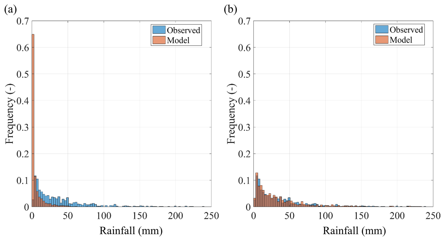
Figure 4 Frequency data distributions of the Observed and Modeled Rainfall Events from the VHR-PRO_IT dataset for the Cervinara station in the observation period: (a) before the application of the bias correction procedure and (b) after the application of the bias correction procedure.

2.3.2 Trend analysis of projected magnitudes

Trend analysis was conducted in two stages: (1) exploring overall changes in rainfall and subsurface characteristics without distinguishing between landslide-triggering and non-triggering events, and (2) analyzing only landslide-triggering events.

Rainfall magnitude, duration, event temporal patterns, and volumetric water content prior to each rainfall event were analyzed on a seasonal basis to identify trends during critical months that contribute to landslide-prone soil conditions. Specifically, mean seasonal projected quantities, along with their standard errors, were analyzed for different periods to capture typical seasonal conditions: Autumn from September to October (SON), marking the onset of the hydrological year; Winter from December to February (DJF), representing an intermediate wet and cold period; Spring conditions from March to May (MAM), preceding the onset of dryer conditions; and (d) Summer from June to August (JJA), indicating the warmest and dryest conditions before the end of the hydrological year.

For the trend analysis we applied a time series decomposition to the projected rainfall data from each climate model at every rain gauge observation point. For this purpose, we used Singular Spectrum Analysis (SSA), a non-parametric technique that separates a time series into meaningful components without assuming a predefined functional form (Golyandina and Zhigljavsky, 2013).

The SSA process begins by reconstructing each rainfall time series into a form that preserves its temporal structure while enabling a detailed examination of its underlying patterns. A 30-year sliding time window was used to capture long-term variability. This transformation allows the data to be expressed as a combination of components that represent different sources of variability.

The transformed data were then analyzed to identify the most important components, i.e. those that contribute most strongly to the overall variability of the series. The leading components, which describe slow and persistent changes, were interpreted as the trend signal. Their selection was guided by their dominant contribution to the total variability and their smooth, monotonic evolution over time. Each identified trend was cross-checked against expectations for long-term variability within the original time series to ensure consistency. The remaining components, which represent progressively smaller contributions, typically correspond to oscillatory patterns (such as seasonal or interannual cycles) or high-frequency noise. Since this study focuses on long-term rainfall changes, these shorter-term fluctuations were not analyzed further. Finally, the selected components were transformed back into the time domain to produce a smoothed representation of the underlying trend. This approach is robust to noise and missing data, making it particularly well suited for detecting long-term signals in climate projections.

Rainfall distribution over time, commonly represented through hyetographs, is known to be related to slope instabilities (D'Odorico et al., 2005). Slope stability is sensitive to both internal and external factors, particularly the soil moisture state prior to a rainfall event (Marino et al., 2020b). However, recent studies indicate that regarding landslide-triggering events, the temporal distribution of rainfall can play an important role, affecting the ground conditions before the onset of the triggering rain event (Natalia and Yang, 2026). Specifically, the effect of rainfall event temporal patterns was assessed by classifying rain events according to their maximum peak intensity (Wu et al., 2006). Figure 5 presents a schematic view of this rainfall-type characterization, according to hyetograph shape. Type 1 (“early-peak”) events concentrate most of the rainfall during the initial phase of the event, with the cumulative total reaching 50 % of the event rainfall within the first 40 % of its duration. Type 2 (“mid-peak”) events exhibit a near-uniform or Gaussian temporal distribution, with cumulative rainfall reaching 50 % approximately midway through the event (between 40 % and 60 % of its duration). Type 3 (“late-peak”) events release most of the rainfall toward the end of the event, with cumulative rainfall reaching 50 % only after 60 % of the duration has elapsed. This classification helps describe the internal temporal structure of rainfall events beyond total depth and duration. More specifically, hyetographs are analyzed for both the triggering rainfall event and the antecedent rainfall event; that is, the one occurring immediately before the triggering event.

In this study, rainfall types are defined as antecedent (${\mathrm{\Phi }}_{\mathrm{a}}^{\mathrm{LS}}$), the event preceding the triggering rainfall, and triggering (Φ^LS). The subscripts 1, 2, and 3 denote the temporal distribution of the rainfall: (1) early peak, (2) mid-peak, and (3) late peak.

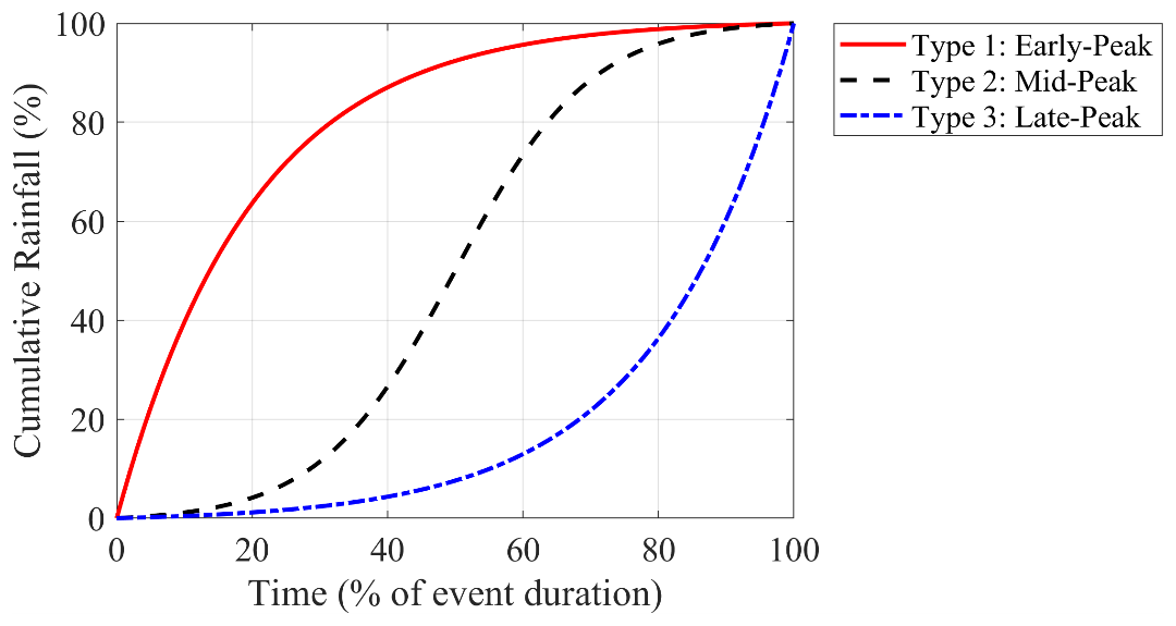
Figure 5 Schematic representation of rainfall event types based on the temporal distribution of cumulative rainfall. The x-axis represents the percentage of event duration, while the y-axis indicates the cumulative percentage of rainfall.

2.4 Analysis of the influence of future climate scenarios on landslide occurrence

Landslide events were identified within the simulations by tracking when the Factor of Safety (FS) drops from a stable state (FS>1.1 to a critical state (FS≤1.1), specifically accounting for the physical delay in how water moves through the soil, similarly as described in Roman Quintero et al. (2025). To ensure statistical accuracy, multiple failures occurring at the same time are treated as a single event unless the slope fully recovers its stability before failing again. This logic categorizes triggers based on their relationship to rainfall: failures during post-storm dry spells are attributed to the “lag” of previous rain (Case 1), failures during active rainfall are tied to the current storm (Case 2), and new rain hitting a slope that is already in a critical state is ignored to avoid redundant counting (Case 3).

The landslide occurrence was studied using two metrics. First, the yearly ensemble landslide frequency λ_LS, defined in Eq. (1).

$$\begin{array}{}\text{(1)}& {\mathit{\lambda }}_{\mathrm{LS}}\left(t\right)={\displaystyle \frac{\mathrm{1}}{N_{\mathrm{EM}}}}\sum _{i=\mathrm{1}}^{N_{\mathrm{EM}}}{N}_{\mathrm{LS},i}\left(t\right)\end{array}$$

where N_LS,i(t) is the number of landslides identified in year t for ensemble member i, and N_EM is the number of ensemble members.

λ_LS was further analyzed in terms of anomalies (Δλ_LS), defined as the difference between the yearly Δλ_LS values and the value at the beginning of the study period (i.e., 2006).

Second, the rainfall-triggered landslide marginal probability (P_LS) was estimated as the number of landslide events divided by the number of rain events, both occurring over a 20-year period at each rain gauge station, and computed as:

$$\begin{array}{}\text{(2)}& P_{\mathrm{LS}}={\displaystyle \frac{N_{\mathrm{LS},\mathrm{20}\mathrm{yr}}}{N_{\mathrm{RE},\mathrm{20}\mathrm{yr}}}}\end{array}$$

where N_LS,20yr is the number of landslides identified over a 20-year period, and N_RE,20yr is the number of rainfall events within the same period. In this study, P_LS was evaluated for the periods 2006–2026 and 2050–2070.

P_LS was further analyzed in terms of the relative change in landslide probability (δP_LS) during 2050–2070 with respect to 2006–2026.

Therefore, the proposed experimental procedure investigates changes in landslide occurrence by accounting for two critical factors influencing the incidence of rainfall-triggered landslides: (i) the effects of rainfall changes projected under different climate scenarios, and (ii) the local rainfall variability within the study area.

The experiment was structured as a 3×3 factorial design combining three climate projection scenarios (RCP 8.5, RCP 4.5, and CTRL) with three groups of rain gauges representing distinct spatial sectors of the study area. Each combination included 27 study units, corresponding to landslide time series derived from the climate ensembles, ensuring statistically consistent results with a test power ≥0.9 (Erdfelder et al., 2009).

The resulting data were analyzed using the Analysis of Variance of Aligned Rank Transformation (ANOVA-ART; Wobbrock et al., 2011) to evaluate the influence of climate change and the spatial and temporal variability of rainfall projections on landslide occurrence. When the ANOVA-ART indicated statistically significant results, post-hoc tests of Estimated Marginal Means (EMMs) were performed to identify significant pairwise differences between climate scenarios and spatial rainfall groups (Lenth, 2025; Searle et al., 1980).

3 Results

3.1 Projected changes in rainfall and soil antecedent conditions

Figure 6 presents the seasonal median values of the trend components for total rainfall, duration, and antecedent volumetric water content, respectively for the different scenarios. Figure 6a presents the time series of anomalies for total rainfall per event during SON, showing opposite trends: negative for the RCP4.5 scenario and positive for the RCP8.5 scenario. Figure 6d shows a positive trend for RCP8.5, while conditions remain relatively stable under RCP4.5 during DJF. Figure 6g shows a slightly negative trend in both scenarios during MAM, similar to Fig. 6j during JJA. In all cases, CTRL exhibits relatively stable conditions.

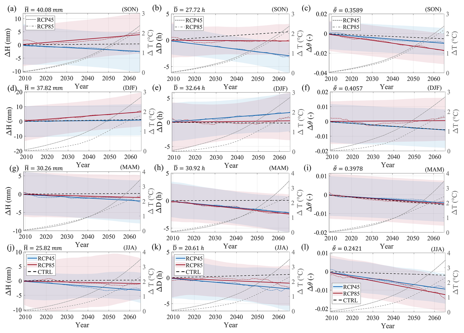
Figure 6 Anomalies in the trend of investigated quantities (dashed lines) and its linear interpolation (solid lines) for: (a, d, g, j) total event rainfall (ΔH), (b, e, h, k) duration (ΔD), and antecedent volumetric water content (Δθ), along with projected temperature shift (ΔT) in the study area on a seasonal basis: (a–c) September, October, November (ON); (d–f) December, January, February (DJF); (g–i) March, April, May (MAM); (j–l) June, July, August (JJA). The shaded regions signify the standard deviation across the climate change ensembles for the RCP4.5 (blue) and RCP8.5 (red) scenarios. Average magnitudes at the beginning of the period 436 are reported in the top-left corner as reference.

Similarly, Fig. 6b presents the anomalies for rainfall event duration, showing a negative trend for RCP4.5 and stable conditions for RCP8.5 in SON. Figure 6e shows stable conditions for RCP8.5, but a positive trend for RCP4.5. Figure 6h, k show a negative trend for both scenarios during MAM and JJA, respectively. In contrast, CTRL exhibits relatively stable conditions, excepting SON.

Likewise, Fig. 6c displays a negative trend in anomalies on volumetric water content prior to rainfall initiation under both the RCP4.5 and RCP8.5 scenarios during SON. Figure 6f shows stable conditions for RCP8.5 but a negative trend for RCP4.5 during DJF. Figure 6i, l show a negative trend in both climate change scenarios. In this case, CTRL also shows a negative trend, although it is generally less pronounced.

Minor trends observed within the CTRL scenario – such as fluctuations in storm duration or soil water content – arise from stochastic variability inherent in the rainfall generation process, exacerbated by the relatively short study period. These fluctuations represent baseline natural noise. While most are significantly less pronounced than the climate change forcing, some stochastic trends occasionally approach the magnitude of climate-driven shifts. This raises a critical question: are the emerging landslide patterns under climate change fundamentally unique, or simply amplified manifestations of this internal variability? Section “Testing the significance of projected landslide changes” investigates this divergence, evaluating whether climate-driven failures represent a statistically significant departure from baseline conditions.

Figure 7 presents a map dividing the area according to the three groups established in Sect. 2.4: Group a – RGa, Group b – RGb and Group c – RGc. Moreover, in the inner tables of the same figure, it displays the direction of the trend in scenarios RCP4.5 and RCP8.5 and the percentage of agreement amongst the ensemble members in brackets (e.g. +(81 %) for total rainfall trend in SON, for group b). These percentages indicate the consensus regarding the sign of the trend; as trends are categorized solely by their direction (positive or negative) without a significance threshold, the remaining percentage inherently represents the proportion of ensemble members projecting a trend in the opposite direction.

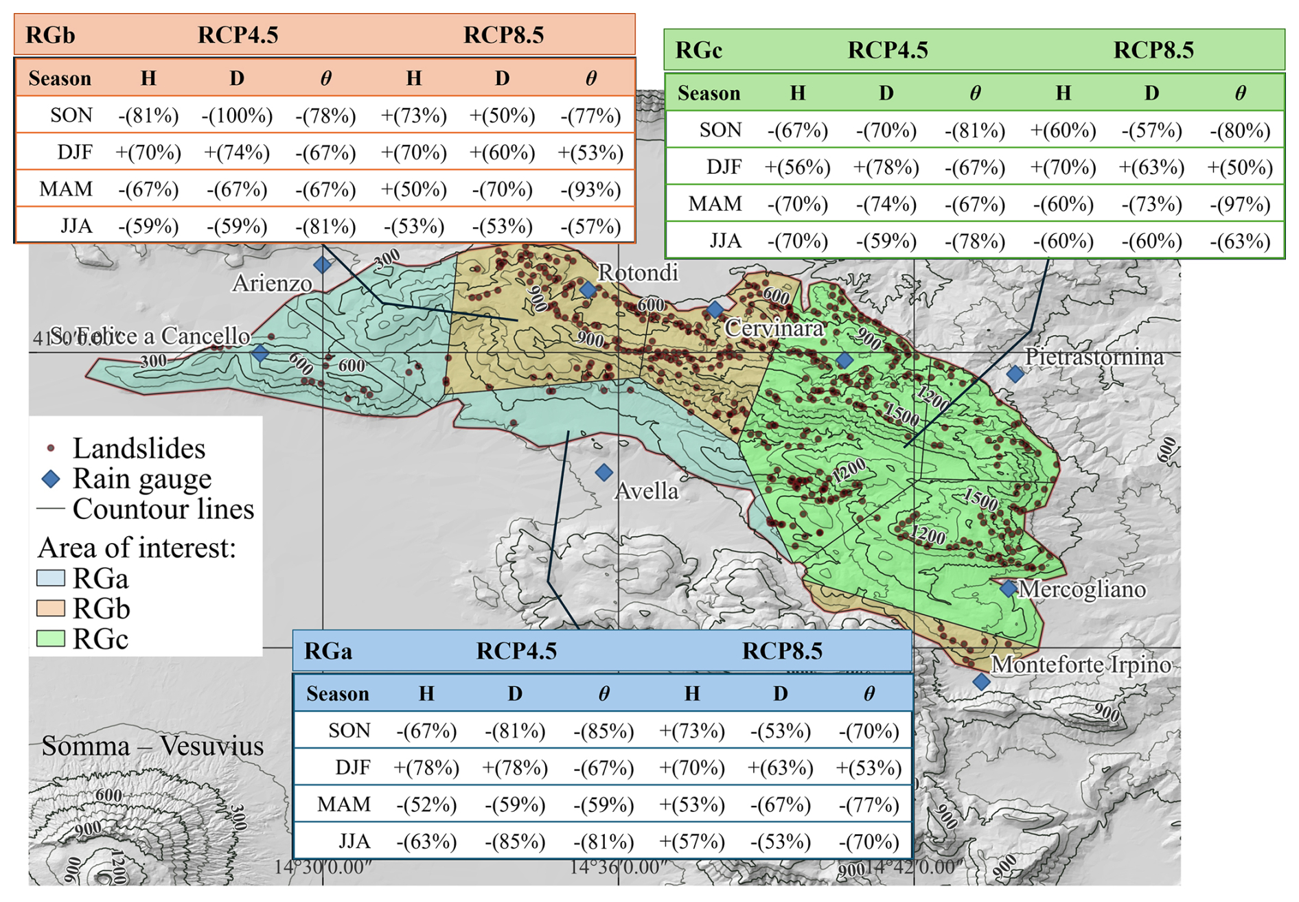
Figure 7 ubregional trend (positive “+” or negative “−”) and percentage of agreement (in brackets) of the ensemble members on rainfall (H), intensity (D) and antecedent volumetric water content (θ), according to RCP4.5 and RCP8.5 climate change scenarios.

Furthermore, Fig. 7 shows the climate change trends and their interaction with spatial variability across the study area, together with model spread among ensemble members. Overall, the entire area exhibits a projected tendency toward smaller and shorter rain events and drier antecedent conditions, reflected in negative trends for event rainfall, duration, and antecedent volumetric water content.

However, both climate change scenarios indicate wetter conditions in DJF, with increases in H and D. Projected trends highlight a marked seasonal contrast, with wetter winters (DJF) and progressively drier spring–summer periods (MAM–JJA). Under RCP4.5, H and D generally decrease in SON, MAM, and JJA but increase in DJF, while θ consistently declines across all seasons. RCP8.5 amplifies these patterns, producing stronger wetting in SON and DJF (up to +73 % agreement for H) and more severe drying in MAM (θ down to −97 %) and JJA. Spatially, Group c exhibits the strongest wetting signal in SON and DJF, whereas Groups a and b show more pronounced drying in MAM. These results suggest an intensification of seasonal contrasts, with stronger storms entering the hydrological year, wetter soils but becoming progressively drier toward summer.

3.2 Projected changes in landslide occurrence

The forthcoming analysis focuses on landslide-triggering rainfall events. Figure 8 shows the trends of temperature anomalies (ΔT) and the ensemble landslide frequency (λ_LS). The figure depicts the co-evolution of climate warming and slope instability under the RCP4.5 and RCP8.5 scenarios. The trend component of the CTRL scenario time series is also shown as a benchmark with current climate conditions. The variability of the variables shown in Fig. 8 is presented in Fig. S2 of the Supplement.

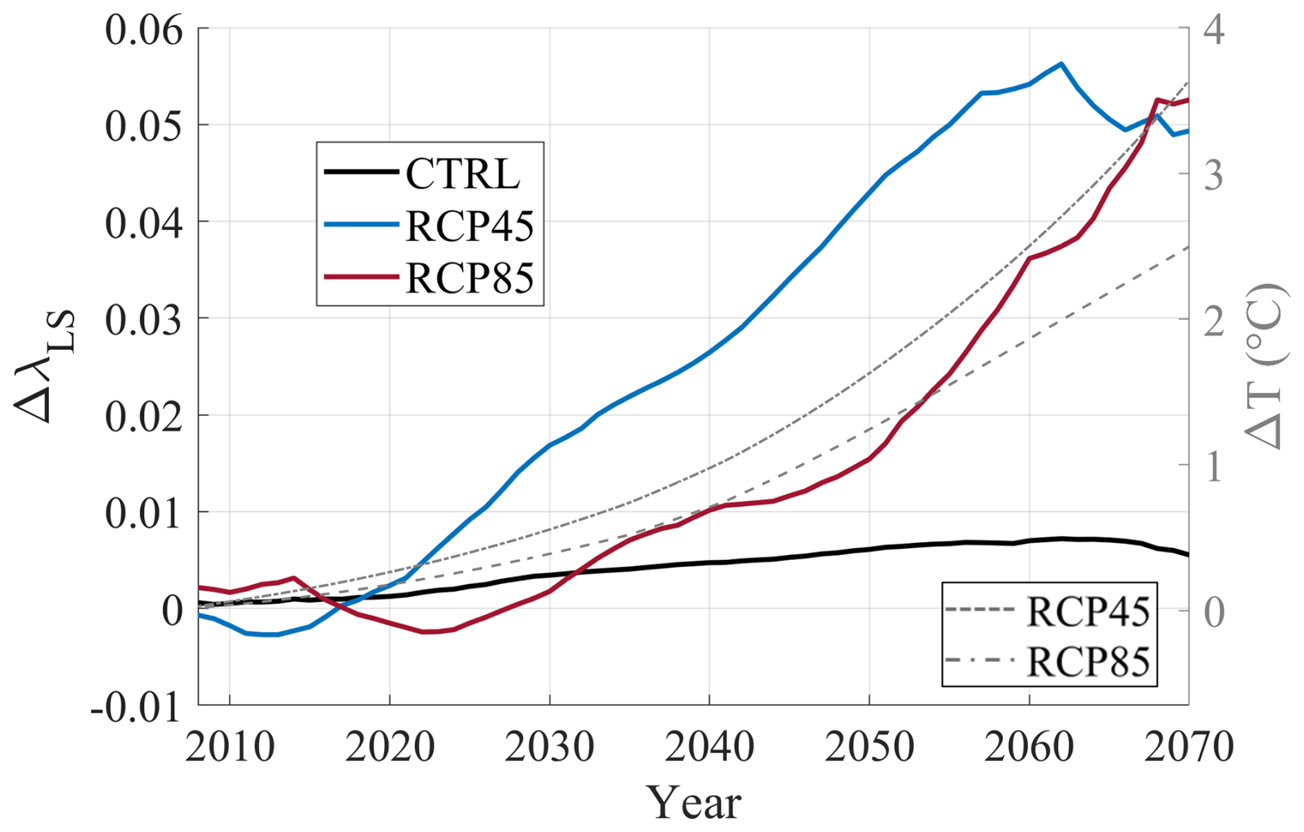
Figure 8 Anomalies on the trend component of the time series of temperature (ΔT) and landslide frequency trend (Δλ_LS) in the study period under RCP4.5 (blue) and RCP8.5 (red) scenarios, based on climate model ensemble simulations. Temperature change (ΔT) represents the anomaly relative to the 2006 baseline.

Figure 9 shows the trend component of λ_LS anomalies relative to the 2006 baseline for each climate change scenario, with dashed lines indicating the ensemble trend and solid lines the linear interpolation for SON (Fig. 9a), DJF (Fig. 9b), and MAM (Fig. 9c). It seems clear that landslide frequency may increase specifically during DJF and MAM periods. In turn, Fig. 10 presents the trends in anomalies of antecedent rainfall type (Fig. 10a, d, g), triggering rainfall type (Fig. 10b, e, h), and total rainfall amount (Fig. 10c, f, i) during landslide-triggering events for the same periods. In both figures mean baseline values are reported on top left side as reference. The variability of the variables shown in Fig. 9 is presented in Fig. S3 of the Supplement.

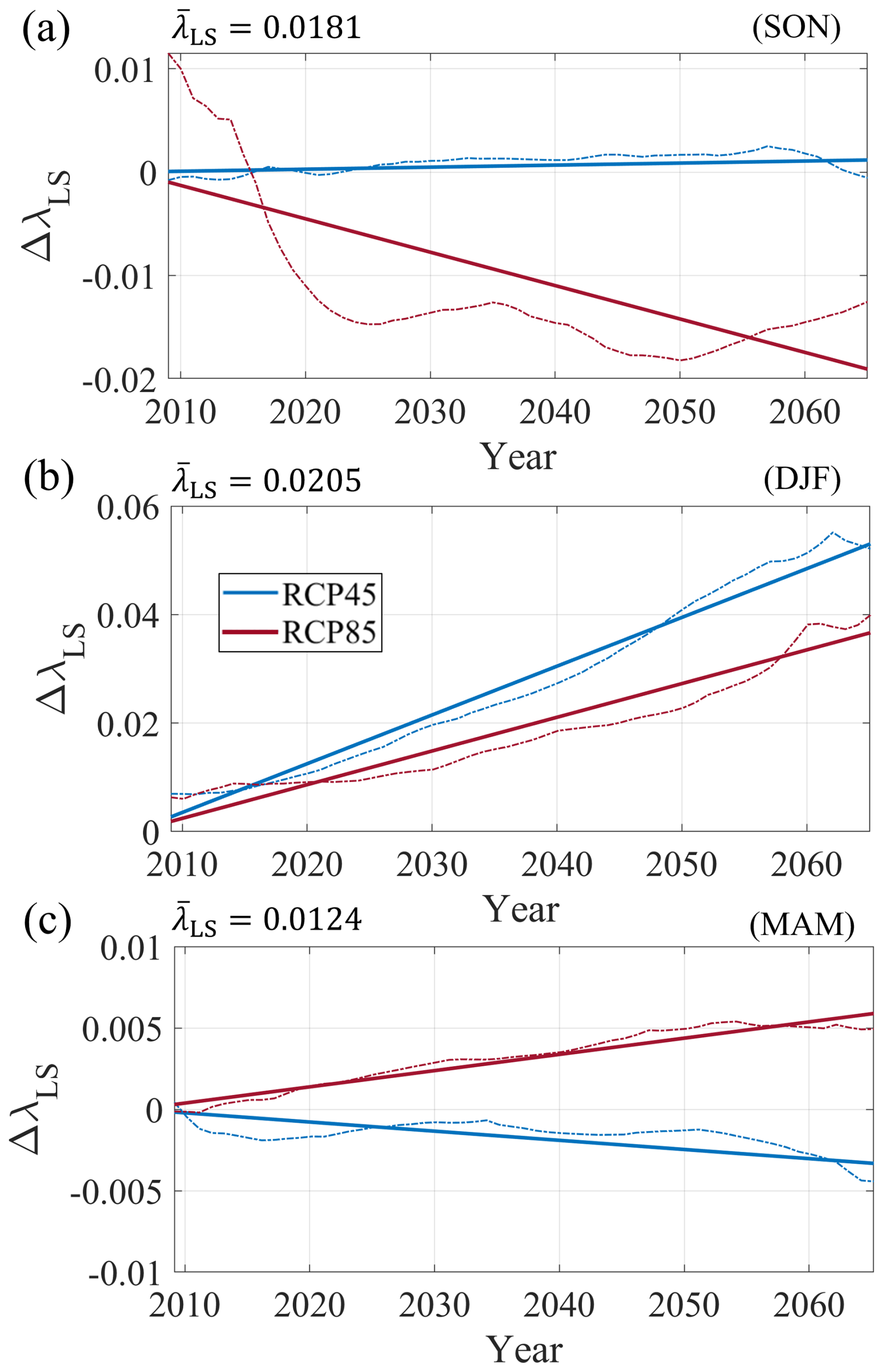
Figure 9 Anomalies on ensemble landslide frequency (Δλ_LS) for the three climate scenarios during the projected period. Panels (a–c) show seasonal trends for ON (a), DJF (b), and MAM (c), comparing RCP4.5 (blue) and RCP8.5 (red). Average landslide frequency (${\stackrel{\mathrm{‾}}{\mathit{\lambda }}}_{\mathrm{LS}}$) at the start of the projected period is presented on top left side of each panel as reference.

From Figs. 9 and 10, it can be seen that under the RCP8.5 scenario there is an increase in λ_LS during DJF and MAM, driven by higher triggering rainfall events, while during DJF the RCP4.5 scenario shows an even stronger increase in λ_LS. In this case, the trend appears to coincide with an increase in antecedent rainfall type 3 and triggering rainfall type 1. Although explored in more detail later, the evolution of landslide occurrences, represented by the rate of change in λ_LS per year, naturally shows spatial variations related to both climate projections and rainfall spatial variability. However, the overall trend is preserved.

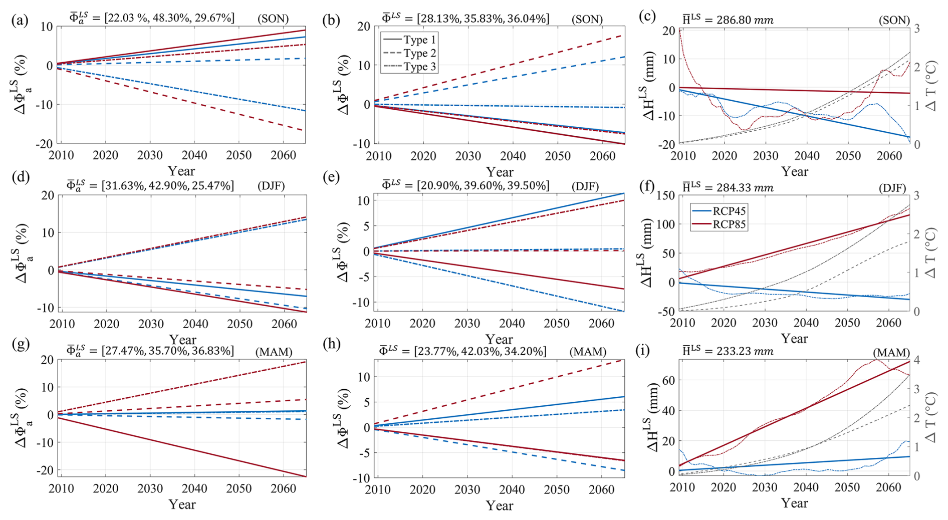
Figure 10 Trend component and linear interpolation of anomalies of: (a, d, g) antecedent rainfall type ($\mathrm{\Delta }{\mathrm{\Phi }}_{\mathrm{a}}^{\mathrm{LS}}$), (b, e, h) triggering rainfall type (ΔΦ^LS), and (c, f, i) total rainfall during landslide triggering events (ΔH^LS) in ON (a–c), DJF (d–f), and MAM (g–h). In (c), (f) and (i) dashed lines represent the trend component values, while solid lines are their linear interpolation. In all other cases lines represent only the linear interpolation of the trend for each rainfall type. Average magnitudes at the beginning of the period are presented on top-left side of each panel as a baseline reference for antecedent rainfall type ${\mathrm{\Phi }}_{\mathrm{a}}^{\mathrm{LS}}=\left[{\mathrm{\Phi }}_{{\mathrm{a}}_{\mathrm{1}}}^{\mathrm{LS}},{\mathrm{\Phi }}_{{\mathrm{a}}_{\mathrm{2}}}^{\mathrm{LS}},{\mathrm{\Phi }}_{{\mathrm{a}}_{\mathrm{3}}}^{\mathrm{LS}}\right]$, triggering rainfall type ${\stackrel{\mathrm{‾}}{\mathrm{\Phi }}}^{\mathrm{LS}}=\left[{\mathrm{\Phi }}_{\mathrm{1}}^{\mathrm{LS}},{\mathrm{\Phi }}_{\mathrm{2}}^{\mathrm{LS}},{\mathrm{\Phi }}_{\mathrm{3}}^{\mathrm{LS}}\right]$, and total triggering rainfall ${\stackrel{\mathrm{‾}}{H}}^{\mathrm{LS}}$.

Figure 11 shows the correlation coefficient between anomalies in trends of landslide frequency and antecedent rainfall types (${\mathrm{\Phi }}_{\mathrm{a}}^{\mathrm{LS}}$), triggering rainfall types (Φ^LS) and total triggering rainfall (H^LS). Direct relationships are indicated by positive correlations in red cells. On the contrary, inverse relationships are indicated by negative correlations in blue cells. Clear direct relationships can be seen with ΔH^LS for RCP8.5 scenario in DJF and MAM. Interestingly, significative increases in landslide frequency coincide with positive correlations with increasing $\mathrm{\Delta }{\mathrm{\Phi }}_{{\mathrm{a}}_{\mathrm{3}}}^{\mathrm{LS}}$ and $\mathrm{\Delta }{\mathrm{\Phi }}_{\mathrm{1}}^{\mathrm{LS}}$. This condition occurs in RCP4.5 scenario during the DJF period.

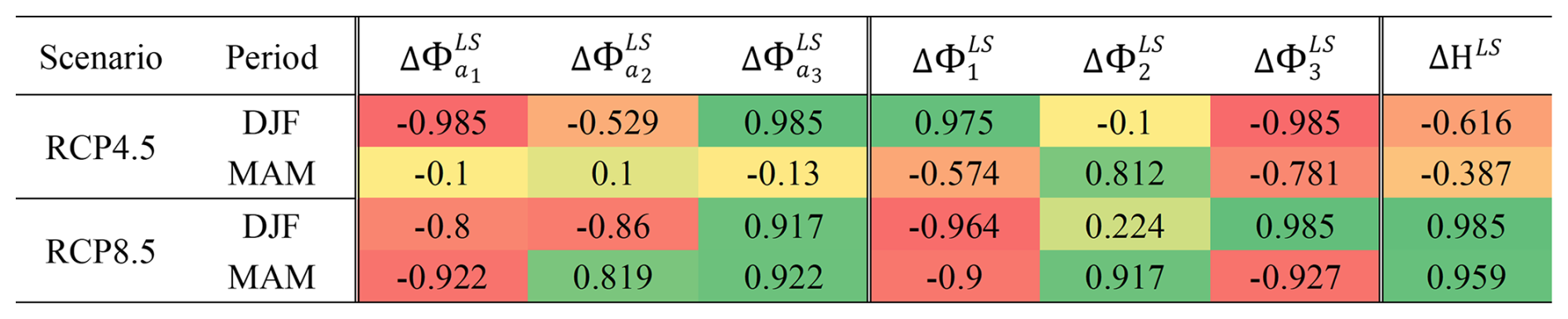
Figure 11 Linear correlation coefficients from the correlations between anomalies in landslide frequency (Δλ_LS) and the anomalies in antecedent rainfall types ($\mathrm{\Delta }{\mathrm{\Phi }}_{a_{\mathrm{1},\mathrm{2},\mathrm{3}}}^{\mathrm{LS}}$), triggering rainfall types ($\mathrm{\Delta }{\mathrm{\Phi }}_{\mathrm{1},\mathrm{2},\mathrm{3}}^{\mathrm{LS}}$) and rainfall (ΔH) during triggering events for the DJF and MAM periods under RCP 4.5, RCP 8.5, and CTRL scenarios. Negative values (blue cells) indicate inverse relationships, while positive values (red cells) indicate direct relationships.

Figure 12 shows the anomalies in antecedent volumetric water content for landslide-triggering events (θ^LS) during the DJF and MAM periods. Specifically, while Fig. 12b shows very subtle changes in θ^LS, Fig. 12a indicates an increasing trend in θ^LS in DJF. This coincides with the absence of a clear correlation (or even an inverse relationship) between Δλ_LS and ΔH^LS, particularly for RCP4.5 during DJF. Under such conditions, less rainfall may be required to trigger landslides as the antecedent wetting front just sets the landslide prone conditions when the triggering rainfall hit the slope. The variability of the variables shown in Fig. 12 is presented in Fig. S4 of the Supplement.

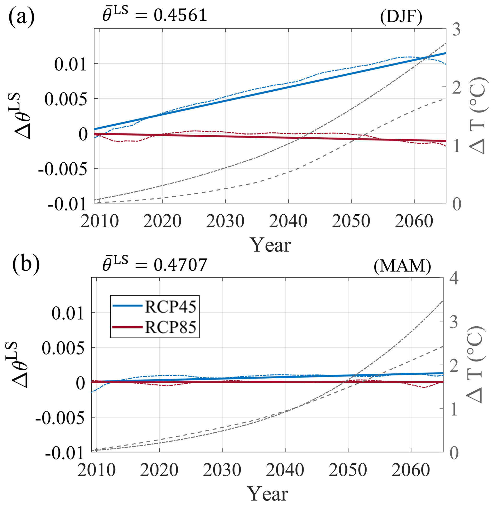
Figure 12 Anomalies of antecedent volumetric water content (Δλ^LS) one hour before the onset of triggering rainfall events in DJF (a) and MAM (b).

Testing the significance of projected landslide changes

As the analyses shown above are tied to the variability expected from subregional spatial rainfall variations and climate modeling, Table 1 presents the results of an Analysis of Variance with Aligned Rank Transformed Data (ANOVA–ART) to statistically validate the findings. Using the number of landslides obtained from the simulations of each ensemble member for the period 2050–2070, the analysis considered three factors: the projected scenario (RCP4.5, RCP8.5 and CTRL), the location within the study area (RGa, RGb and RGc), and their interaction.

Table 1 Analysis of Variance with Aligned Rank Transformed Data (ANOVA-ART) of the projected number of landslides between 2050 and 2070, for each projected climate scenario and geographical position within the subregion. Levels of significance: (iii) α<0.001 (ii) α<0.01 (i) α<0.05.

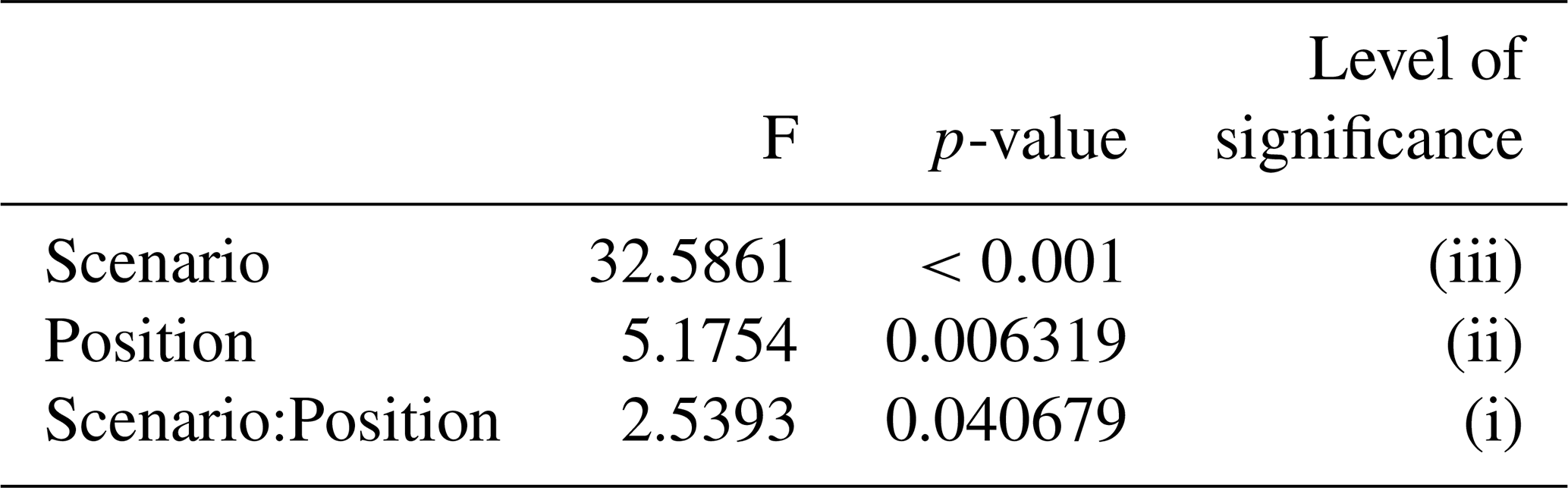
All factors show statistical significance, with the strongest effect confirming that the number of landslides toward the end of the period is primarily influenced by climate change scenarios. This is followed by location, which shows significant spatial differences within the study area. Finally, significant effects are also observed from the interaction between climate scenario and location.

Given the statistical significance of the ANOVA–ART test, the Estimated Marginal Means (EMMs) method was applied as a post-hoc test to explore what are the climate scenarios and geographical positions showing sufficient statistical differences in triggering landslides at the end of the projected period. Table 2 shows the p-values associated with the test and the pairwise comparison between climate scenarios and different geographical positions characterized by the rain gauge group (i.e. RGa, RGb and RGc).

Table 2 p-values from the statistical comparison of the projected number of landslides between 2050 and 2070 across different climate scenarios and geographical positions, using the Estimated Marginal Means (EMMs) method.

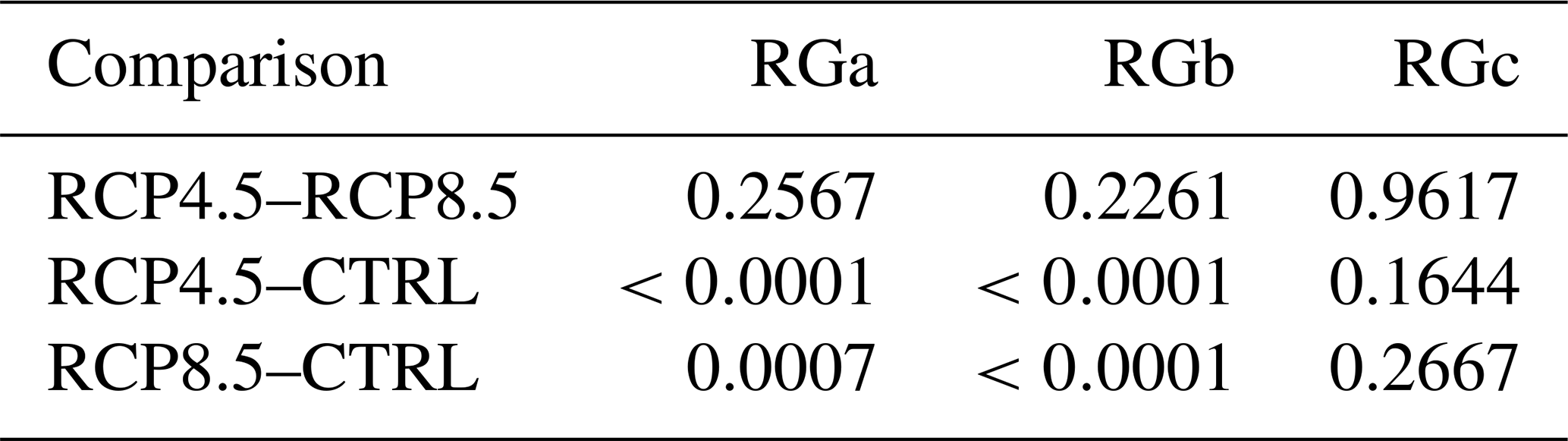
The results from Table 2 indicate that scenarios considering climate change conditions (i.e. RCP4.5 and RCP8.5) produce statistically significant differences in the number of landslides at the end of the studied period when compared with the CTRL scenario. However, the direct comparison between RCP4.5 and RCP8.5 does not reveal any statistically significant differences by the end of the projected period (p>0.22 for all rain gauge groups).

Interestingly, rainfall spatial variability plays a key role in some cases. For rain gauge groups RGa and RGb, both RCP4.5–CTRL and RCP8.5–CTRL comparisons yield highly significant results (p<0.001), confirming that climate change conditions are likely to increase landslide occurrence in these regions. In contrast, RGc shows no statistically significant differences under either climate scenario (p>0.16), suggesting lower sensitivity to projected climate change in that sub-region.

This pattern is consistent with the marginal landslide probability (P_LS) across the area for both RCP4.5 and RCP8.5. The maximum P_LS is $\sim \mathrm{7}\times {\mathrm{10}}^{-\mathrm{4}}$ in RGa, ∼0.01 in RGb, and ∼0.023 in RGc. As shown in Fig. 13, RGa contains the fewest landslides (22 units), followed by RGb (207 units) and RGc (238 units). This spatial pattern mirrors mean rainfall per event, as rain events in RGa have on average ∼22 mm per event, RGb ∼30 mm per event, and RGc ∼37 mm per event. However, Fig. 13 also highlights that the relative increase in landslide probability (δP_LS) between 2006–2026 and 2050–2070 (considering both climate change scenarios) is highest in RGa and lowest in RGc, indicating a proportionally stronger climate change signal in the less-affected western sector, than in the eastern sector. Figure 13 displays the maximum shift in P_LS within each group.

4 Discussion

Projected changes in rainfall and subsurface conditions indicate that, overall, the area is trending toward drier soil conditions, particularly in autumn, spring and summer. These findings, consistent with previous studies conducted at larger scales, suggest that even at local and subregional scales the area tends towards aridity, but accompanied by significant rainfall variability driven by changes in atmospheric conditions and its dynamics (Raffa et al., 2023; Rajczak and Schär, 2017). The analysis of projected rainfall events at the nine rain gauge stations in the area clearly indicates that, even if the rainfall proportion remains (i.e. Rainfall in RGc is greater than rainfall in RGb and greater than rainfall in RGa), change signals may be stronger in some subregions than in others. However, the resolution of most existing regional climate simulations in the analyzed ensemble members is relatively coarse (∼ 12.5 km), imposing a limitation to these results, particularly for convective-scale rainstorms (∼ 2–3 km), a capability that would be desirable for detailed studies supporting landslide-scale hazard assessments.

Nonetheless, the assessment of climate change impacts on rainfall-triggered shallow landslides in the area shows that, despite the trend toward drier conditions, a projected increase in landslide occurrence is expected. In this study, future projections indicate a stronger increase in landslide frequency under the RCP4.5 scenario compared to the RCP8.5 scenario. Similarly, a notable study focusing on the nearby region of Calabria (southern Italy) projects a regional increase in the number of landslides, with a stronger rise under RCP4.5 than under RCP8.5 for the period 2036–2065 (Gariano et al., 2017).

As seen in the results, changes in landslide occurrence are closely linked to changes in rainfall patterns. These conditions, which affect both triggering and antecedent rainfall events, drive variations in meteorological landslide triggering mechanisms. Under RCP8.5 conditions, landslide-triggering events are associated with a direct increase in triggering rainfall. In contrast, the RCP4.5 scenario reveals a more complex “perfect storm” mechanism: a combination of Type 3 antecedent rainfall (late-peak) and Type 1 triggering rainfall (early-peak). This alignment is physically significant: late-peak antecedent events ensure that soil moisture remains at near-saturation levels immediately before the onset of the next storm, while early-peak triggering events deliver maximum intensity when the slope is at its most vulnerable. This specific interaction between hyetograph shape and slope stability has been observed in laboratory settings and back-analyses of historical failures, where advanced (early-peak) rainfall patterns were found to reduce the factor of safety more rapidly than delayed patterns (Jayakodi et al., 2023; Ng et al., 2001).

Regarding triggering conditions, clear changes are evident even in landslide records. While total annual rainfall may show mixed signals, recent observational studies have begun to detect subtle shifts in sub-daily rainfall distributions, with a tendency toward more “pulsing” or “peaked” events in Mediterranean and subtropical climates (Natalia and Yang, 2026). Historical data show a reduction in the average and maximum cumulative event rainfall required to initiate landslides in nearby regions (Gariano et al., 2015). This suggests that slopes are becoming more sensitive to instability, as shown in this study, due to progressively worsening predisposing conditions. As a result, rainfall patterns appear to be evolving in a way that is more conducive to triggering, regardless of total rainfall magnitude. Notably, these rainfall patterns are captured here in the RCP4.5 ensemble.

A key role is played by antecedent soil moisture conditions. Our findings suggest that the strong correlation between landslide frequency and rainfall timing (Fig. 11) is mediated by the soil's hydrological state. Although changes in rainfall magnitudes and intensities have been demonstrated, critical antecedent soil conditions are linked to relatively stable geomorphological settings. However, the shift toward Type 3 (late-peak) antecedent rainfall effectively “primes” these settings by maximizing infiltration just before the triggering event begins. Studies in southern Italy have shown that soil water content, relative to field capacity, controls infiltration processes and landslide triggering mechanisms (Roman Quintero et al., 2023, 2025). The synergy between rainfall timing and soil moisture – where the internal structure of the rain event compensates for a decrease in total volume – is a critical finding that aligns with recent high-resolution climate modeling suggesting that the “inter-arrival” time and internal timing of storms are becoming more influential than total seasonal depth (Semnani et al., 2025). Preliminary analyses of rainfall intensity–duration thresholds for shallow landslides in Basilicata (Southern Italy) further indicate that, in some cases, soil moisture exerts a strong control on triggering, supporting this hypothesis (Lazzari et al., 2018). However, establishing critical soil moisture conditions must rely on a physically based rationale, which is more likely to be achieved in relatively well-characterized geological and morphological settings, such as the study area presented here (Bezak et al., 2021; Marino et al., 2020b; Roman Quintero et al., 2025).

Overall, the evidence points toward an increased future landslide risk in the study area, driven by either a projected rise in triggering rainfall or changes in the rainfall conditions required for triggering. However, recent studies using climate projections highlight uncertainties arising from variability within projected ensemble members (Buonacera et al., 2025; Semnani et al., 2025). This study shows that, despite ensemble variability, trends consistently indicate an increase in landslide occurrence under future climate projections, supported by strong statistical evidence demonstrating significant differences between current observed climate conditions (CTRL) and climate change scenarios (RCP4.5 and RCP8.5) when analyzing the landslides occurring at the end of the study period (2050–2070). These results also extend to rainfall spatial variability at the subregional scale, with particularly pronounced changes in areas historically less affected by landslides (i.e., RGa), but weaker signals in areas already prone to landslides and characterized by the highest recorded and projected rainfall amounts in the region (i.e., RGc). However, although a faster rise in landslide frequency is observed under RCP4.5 compared to RCP8.5, there is no statistical evidence that this difference remains significant by the end of the study period.

5 Conclusions

We examined landslide occurrence in the Partenio Mountains (southern Italy) for 2006–2070 using EURO-CORDEX rainfall projections under RCP4.5 and RCP8.5, downscaled and bias corrected with observations from nine rain gauges (2006–2023). Landslide triggering was analyzed with a calibrated 1D Richards infiltration model and stepwise stability assessment. The same procedure was applied to a synthetic rainfall dataset (CTRL) generated with a stochastic model reproducing observed rainfall conditions.

We conclude that projected rainfall and subsurface changes indicate a general trend toward drier soil conditions, particularly in autumn, spring, and summer, yet accompanied by significant spatial variability at the subregional scale. Despite this drying trend, landslide occurrence is projected to increase, with RCP4.5 showing a stronger rise in frequency than RCP8.5 up to mid-century, although differences between the scenarios are not statistically significant by 2050–2070, both scenarios showed significant differences with the CTRL scenario, representing currently observed conditions.

A further analysis of meteorological triggering mechanisms shows that, under RCP8.5, landslides are mainly associated with direct increases in total event rainfall. Under RCP4.5, however, the combination of wetter antecedent conditions, driven by delayed seasonal rainfall peaks, and earlier triggering rainfall peaks produces stronger destabilizing effects. Antecedent soil moisture therefore remains a critical control on landslide initiation, often exceeding the influence of total rainfall changes. As rainfall patterns shift, slopes become increasingly sensitive, with failures potentially triggered by smaller rainfall amounts due to elevated antecedent soil moisture. Consequently, projected changes in precipitation patterns cannot be always directly extrapolated to landslide occurrence: shifts in the return period of extreme rainfall events do not necessarily translate into equivalent changes in landslide return periods.

Taken together, these findings demonstrate that the interaction between climate change and slope hydrological processes can alter slope instability signal even under an overall drying trend, primarily through shifts in rainfall timing and intensity that alter antecedent soil conditions, specifically in extreme events. The consistent increase in projected landslide occurrence across scenarios and subregions highlights the sensitivity of the landscape to evolving hydrometeorological dynamics. This study therefore provides quantitative and process-based evidence that future landslide hazard may intensify not simply because of how much it rains, but because of when and how rainfall occurs. The results align with recent investigations in nearby regions, strengthening the emerging consensus that changes in rainfall patterning, rather than totals alone, will play a decisive role in shaping slope stability under future climate conditions. These insights underscore the need for climate-resilient risk management strategies that explicitly account for rainfall pattern variability and antecedent moisture dynamics in landslide-prone areas.