Deep Learning Emulation of Multivariate Climate Indices: A Case Study of the Fire Weather Index in the Iberian Peninsula

The Fire Weather Index (FWI) is an essential multivariate climate index for assessing wildfire risk and the associated impacts of climate change, as it provides a quantitative measure of wildfire danger by integrating different critical near-surface fire-weather variables, namely air temperature, relative humidity, wind speed, and precipitation. FWI calculation depends on instantaneous data representing noon local standard times, which are often unavailable in many climate data repositories – particularly in climate projections. In these instances, a “Proxy” of actual FWI is often used, applying the same FWI formulation to daily aggregated values (mean, max, or min), despite known limitations in capturing extremes and temporal dynamics.

This study investigates the use of deep learning (DL) models to emulate the reference FWI over the Iberian Peninsula – a predominantly Mediterranean and fire-prone region – using only daily inputs. The emulators are trained and evaluated using ERA5-Land data, which, while not observational ground truth, provides a consistent and high-resolution dataset suitable for controlled inter-comparison. The focus is not on validating FWI against observations, but on assessing the ability of DL models to reproduce the reference FWI more accurately than traditional proxy approaches, using the same input data source.

Our results show substantial improvements in spatial accuracy, preservation of temporal sequences, and detection of extreme fire danger events when compared with the corresponding Proxy version. Furthermore, after evaluating different combinations of input variables for DL model training, we find that precipitation can be excluded without substantially affecting accuracy – especially for the upper part of the distribution – an important insight given the challenges climate models face in representing precipitation. These findings highlight the potential of deep learning tools to enhance the usability of FWI in contexts where sub-daily data are unavailable, and set the stage for the emulation of other multivariate climate indices, which are vital for climate impact studies, spatial planning and management, and adaptation decision-making.

1 Introduction

Fire is a global phenomenon that has shaped ecosystems since the emergence of land vegetation, influencing vegetation structure, the carbon cycle, and climate (Bowman et al., 2009). From a human perspective, wildfires can cause severe ecological damage, threaten lives and infrastructure, and degrade air and water quality, with far-reaching social and economic consequences (Bowman et al., 2017; Pausas and Keeley, 2021).

Fire danger indices are essential tools for wildfire risk assessment and climate impact studies. By integrating key atmospheric variables – such as temperature, humidity, wind speed, and precipitation – into a single, physically interpretable indicator (Fugioka et al., 2009; Yu et al., 2023), these indices support fire management agencies in resource allocation and early warning systems (Di Giuseppe et al., 2020). They also help researchers understand how climate change alters fire-weather patterns (Bedia et al., 2015; Jolly et al., 2015; Bento et al., 2023; Santos et al., 2023; Gincheva et al., 2024) informing adaptation strategies and policy decisions in fire-prone regions (Costa et al., 2020; DaCamara et al., 2024).

Among the various fire-weather indices worldwide, the Canadian Fire Weather Index (FWI, van Wagner, 1987) is one of the most widely adopted globally. In Europe, it underpins the European Forest Fire Information System (EFFIS San-Miguel-Ayanz et al., 2013) and has been extensively used for the estimation of fire danger in vulnerable regions (Camia and Amatulli, 2009), such as Iberia (Santos et al., 2023), as well as for the assessment of future climate change scenarios in the Euro-Mediterranean region (Bedia et al., 2014a; Dupuy et al., 2020) and the Iberian Peninsula (Bento et al., 2023).

Although the adoption of the FWI presents clear advantages for effectively characterizing fire danger weather situations, it also poses some hurdles from an implementation point of view. One significant challenge is that the FWI was originally designed for noon local standard time (LST) conditions, representing the highest fire danger time in mid-latitude regions. This means it requires instantaneous noon time input data of near-surface air temperature, relative humidity, 10-m wind speed and last 24 h accumulated precipitation (Lawson and Armitage, 2008). However, such specific noon data are often missing from observational records. Furthermore, climate model databases quite often do not include sub-daily outputs due to the massive storage requirements (e.g. the Earth System Grid Federation –ESGF–, Cinquini et al., 2014), thus preventing the direct calculation of FWI from climate model simulations.

To circumvent the lack of instantaneous data, daily mean aggregated inputs have been commonly used for FWI estimation, in particular to obtain future projections from model simulations. However, the resulting daily mean FWI proxies cannot be reliably transformed to match their instantaneous counterparts, leading to inconsistent future projections (Herrera et al., 2013). Consequently, approximations are often employed to minimize FWI distortion. One of the pioneering studies in this area utilized different daily proxy variables for FWI calculation from climate model outputs, comparing various combinations of minimum relative humidity and maximum temperature as surrogates for noon-time outputs. This approach aimed to minimize the distortion of the climate change signal in the reference FWI, using simulations from a regional model for both historical and a moderate future warming scenario (Bedia et al., 2014a). Since then, other studies have adopted proxies to produce more accurate FWI projections (Abatzoglou et al., 2018; Bento et al., 2023; Matteo et al., 2025), as a practical solution given the unavailability of more precise data. Despite all these efforts, the approximate version of the FWI inevitably presents certain deviations from the original version that introduce added uncertainty (Bedia et al., 2014a; Matteo et al., 2025).

Emulation offers a promising alternative in this context. Recent advancements in machine learning techniques, particularly deep learning (DL), across various fields suggest that these sophisticated nonlinear models have the potential to effectively represent and capture the intricate structures and nonlinear dynamics inherent in Earth systems (Duffy et al., 2023), including numerical model climate predictions (Rampal et al., 2024) and applications to downscaling (Baño-Medina et al., 2022; Bushenkova et al., 2024; Li et al., 2025; Johannsen et al., 2024; Soares et al., 2024), among others. In this new framework, the emulation function is determined by the neural network's coefficients, allowing for varying topologies to produce different plausible fields (Baño-Medina et al., 2024). This opens up a broad area of research where various techniques and architectures can be compared to evaluate their suitability for specific problems. It also introduces new challenges related to model interpretability, requiring methods of eXplainable Artificial Intelligence (XAI) that reveal how DL models make decisions. Such approaches play a key role in establishing the credibility of the outcomes among users (Dramsch et al., 2025) and for gaining valuable insights into the most influential variables and the physical interpretation of model's functioning (Yang et al., 2024; Baño-Medina et al., 2025). Among the variety of approaches available, saliency maps emerge as valuable tools aiding in the design and evaluation of DL climate downscaling approaches in general (González-Abad et al., 2023), and have been successfully used to unravel DL-based FWI predictions in previous studies (Mirones et al., 2025).

In this study, we explore the emulation of the Fire Weather Index (FWI) using DL models to approximate the index's behavior as closely as possible with commonly available input variables whose temporal frequency (daily) does not match the definition of the “reference FWI” (based on instantaneous noon local standard times). We build upon the reference FWI and the optimal Proxy FWI version presented in Bedia et al. (2014a), which has been widely used in subsequent studies. We compare the emulation of the reference FWI using different combinations of input variables (hereafter predictor sets), including inadequate (daily mean), incomplete (removing some input variables), or suboptimal temporal frequency inputs (i.e. daily minimum relative humidity), which are more commonly available than the required instantaneous data. We test various DL model architectures and topologies and utilize XAI techniques, such as saliency maps, to provide end users and practitioners with a physical understanding of the emulation process.

Our results indicate that DL emulators outperform the traditional Proxy approach in all validation aspects, including spatial representation, preservation of the temporal sequence, and detection of extreme fire danger conditions. The daily mean inputs, which are most widely available in public repositories, are adequate for accurately emulating the reference FWI using the developed DL methods. Furthermore, our findings suggest that precipitation can be omitted from the predictor set without significantly compromising FWI representation accuracy. Overall, we demonstrate that by leveraging simpler inputs, DL emulators can enhance the accessibility and applicability of FWI in impact studies, facilitating a more efficient and widespread use in climate impact studies and decision-making.

In addition, we present a concise set of preliminary experiments on the emulation of the individual fuel-moisture codes (FFMC, DMC, DC). These initial results confirm that FFMC and DMC can be emulated with high fidelity using daily inputs – even when precipitation is excluded – whereas the DC shows a somewhat stronger sensitivity to the presence of precipitation in the predictor set due to its long-term moisture memory. Nonetheless, given that the primary objective of this first study is the emulation of the FWI itself, which integrates the combined effect of all sub-indices and is the most widely used fire-danger indicator in climate and impact research, we restrict our detailed analysis to the FWI while deferring a comprehensive component-level evaluation to a forthcoming companion work.

2 Data and Methods

2.1 Input Data

All data used in this study were obtained from the ERA5-Land database (Muñoz-Sabater et al., 2021), distributed by the Climate Data Store (CDS) of the Copernicus Climate Change Service (Buontempo et al., 2022). ERA5-Land is a high-resolution reanalysis dataset produced by the European Centre for Medium-Range Weather Forecasts (ECMWF). It offers detailed information on land surface variables, providing a consistent view of their evolution over several decades. ERA5-Land features a finer spatial resolution of approximately 9 km grid spacing, compared to ERA5 (∼25 km Hersbach et al., 2020). It covers data from January 1950 to the present, with an hourly temporal resolution. The dataset includes various land surface parameters (such as soil moisture, soil temperature, snow cover, and surface runoff) to control the simulated land fields, ensuring the data remains accurate and consistent. ERA5-Land uses atmospheric variables from ERA5, like air temperature, wind speed and humidity, and presents hourly temporal resolution, thus providing the necessary input variables for the calculation of both reference and Proxy FWI versions, as well as the different predictor sets used in this study (Sect. 2.3).

2.2 Fire Weather Index calculation

The reference noon LST FWI is calculated from ERA5-Land daily records of four near-surface meteorological variables measured at 12 UTC (∼ noon time in the Iberian Peninsula): 24 h accumulated precipitation, instantaneous wind speed, relative humidity, and temperature. These inputs are processed via a set of empirical equations that yield six intermediate components characterizing fuel moisture dynamics across different fuel layers (van Wagner, 1987; Stocks et al., 1989), the influence of wind on fire spread, and the total fuel available for combustion. These components are then integrated to compute the FWI, a dimensionless index representing potential fire intensity under given meteorological conditions for a reference fuel type (mature pine stands).

Beyond the four meteorological inputs required at noon LST, the Canadian FWI System relies on six sequential sub-indices that describe fuel moisture conditions and potential fire behavior (van Wagner, 1987; Stocks et al., 1989; Lawson and Armitage, 2008). Three of them (FFMC, DMC and DC) represent moisture contents at increasing depths of the forest floor and respond to atmospheric drivers at markedly different timescales.

The Fine Fuel Moisture Code (FFMC) characterizes the moisture content of surface litter and fine fuels, which react on hourly–daily timescales to changes in temperature, relative humidity and wind speed, as well as to even small rainfall amounts due to their limited water-holding capacity. FFMC largely governs ignition likelihood and short-term fluctuations in fire danger.

The Duff Moisture Code (DMC) represents the moisture content of moderately deep organic layers in the upper duff. Its evolution reflects medium-term drying (days to weeks), driven primarily by temperature and relative humidity, and decreases only when precipitation exceeds an effective infiltration threshold. The DMC modulates the potential for sustained fire spread once ignition occurs.

The Drought Code (DC) reflects the long-term moisture content of deep, compact organic horizons that respond over weeks to months. The DC accumulates persistent atmospheric moisture deficits and only decreases when substantial or prolonged precipitation is able to percolate into deeper layers. As such, it is a key indicator of seasonal-scale drought and deep-burning potential. These different memory timescales explain the unequal sensitivity of the moisture codes to the meteorological drivers (Wotton, 2009).

The three moisture codes are combined into two intermediate fire-behavior indices. The Initial Spread Index (ISI) combines FFMC with wind speed to estimate the expected rate of fire spread immediately after ignition. The Buildup Index (BUI) integrates DMC and DC to represent the total amount of fuel available for combustion, accounting for both medium- and long-term moisture deficits. Finally, the Fire Weather Index (FWI) combines ISI and BUI through a nonlinear formulation to estimate potential fire intensity for a standard fuel type.

A practical consideration arises from the different response times and memory effects of these components. While the FWI system uses default initial values, leading to a short spin-up period, this transience is typically negligible during the fire season due to rapid stabilization and the minimal influence of snowmelt on moisture inputs (Bedia et al., 2018).

2.3 Predictors Sets

The reference FWI is computed directly from instantaneous meteorological variables at 12:00 UTC (approximately noon local standard time in Iberia), as defined in the standard FWI formulation (see Sect. 2.2). In contrast, the predictor sets used to train the DL emulators (P0, P1, P2) consist of different temporal aggregations and/or preprocessing of these same meteorological variables. Specifically, the emulators are provided with daily aggregated variables (daily means, daily minima/maxima, together with 24 h accumulated precipitation) rather than instantaneous noon values. This distinction is essential for interpreting emulator performance: the DL models learn to recover a noon-time fire weather signal from daily-aggregated inputs, which is an inherently different (and harder) task than the direct FWI computation. Reported errors reflect this added complexity and should not be interpreted as a simple approximation error.

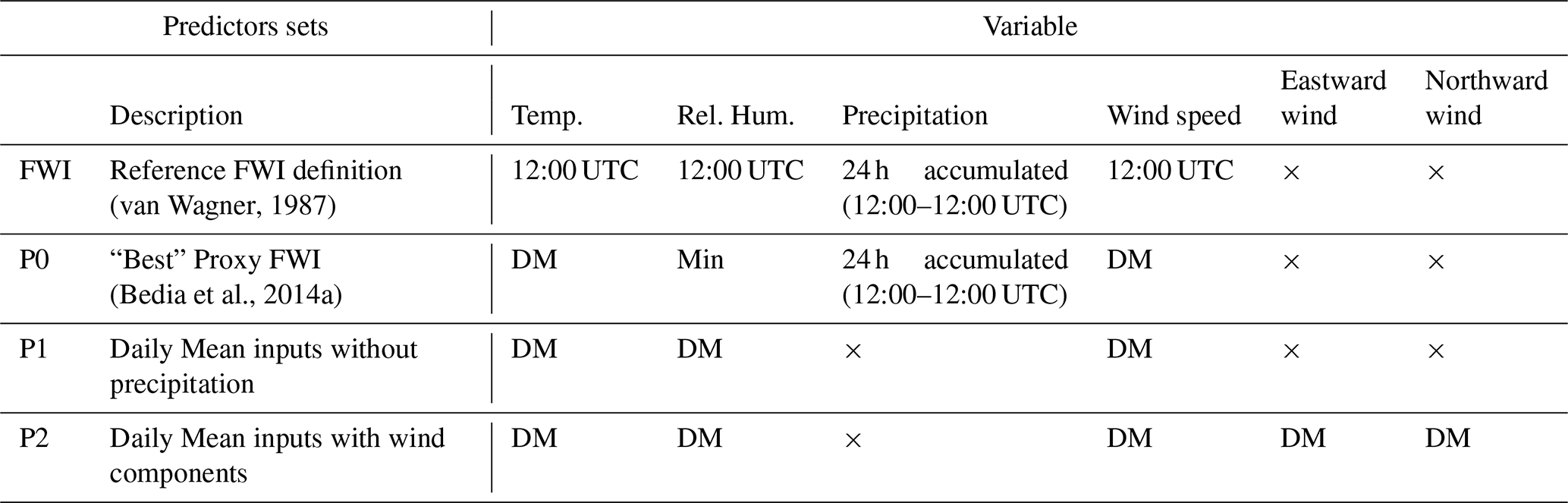
To emulate the reference FWI, we consider several predictor sets derived from ERA5-Land, summarized in Table 1. The initial experiments use P0, which builds on the same set of variables used in the optimal FWI approach from Bedia et al. (2014a) (hereafter Proxy FWI). This allows us to assess whether the DL models can more accurately replicate the FWI transfer function when provided with the same predictors as the Proxy FWI. Accordingly, P0 includes 24 h accumulated precipitation, daily mean air temperature and wind speed, and minimum relative humidity. Proxy FWI is derived from the standard FWI formulation using the latter set of variables. The use of minimum relative humidity in P0 ensures the fairest possible comparison with Proxy FWI. However, in predictor sets P1 and P2, we intentionally replace minimum relative humidity with daily mean relative humidity. This is motivated by the fact that daily mean variables are more consistently provided by climate model outputs and reanalysis datasets, and we wanted to examine the performance of the emulator under such predictor-limited cases. Precipitation poses an additional challenge: it is one of the most difficult variables for climate models and reanalyses to represent reliably, due to its strong spatial and temporal variability, its dependence on complex physical processes, and the influence of multiple interacting factors. To examine whether robust performance can still be achieved in its absence, we exclude precipitation from predictor sets P1 and P2. Finally, in P2 we tried measuring the impact of using wind speed module versus wind speed zonal components, which could be relevant when determining fire danger. Other predictors sets have been tested, such as P1 using minimum relative humidity instead daily mean relative humidity or P0 including the 24 h precipitation, without any added value compared to the configurations mentioned in the manuscript. These experiment results are shown in Fig. D2.

(van Wagner, 1987)(Bedia et al., 2014a)

Table 1 Summary of the predictor sets assessed in this study. 12:00 UTC correspond to instantaneous model outputs verifying at that time. DM corresponds to Daily Mean values, and Max/Min to Daily Maximum/Minimum values. Precipitation is the daily (last 24 h) accumulated value, from 12:00 to 12:00 UTC. Cells marked with × indicate that the variable is not included in the corresponding predictor set. The “FWI” row indicates the instantaneous noon local standard time (LST) variables required by the standard FWI definition. The predictor sets P0, P1, P2 represent temporal aggregations or modifications of the noon LST variables, such as daily means, which are far more widely available across reanalysis and climate datasets. This motivates the emulation approach: rather than requiring instantaneous noon inputs, the emulators allow FWI to be derived directly from these more accessible variable forms.

2.4 Deep Learning Methods

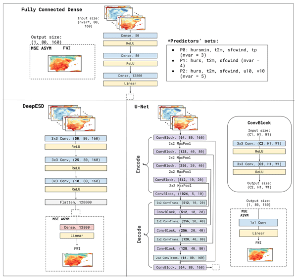
In this section, we briefly describe the DL architectures trained in this study. A visual summary of their topologies is presented in Fig. 1. The selected architectures include the Fully Connected Dense (FCD) model, chosen as benchmark for its relative simplicity, as well as DeepESD and U-Net, which have been recently introduced in the literature for climate downscaling (Baño-Medina et al., 2022; González-Abad et al., 2023; González-Abad and Gutiérrez, 2024). Alternative architectures, such as Convolutional Long Short-Term Memory (ConvLSTM), were also evaluated. However, owing to their inferior performance relative to the selected architectures and their greater computational demands, they are not presented in this manuscript. The DL models are tasked to learn a mapping between different sets of FWI-related input variables (Table 1) and the reference FWI over the Iberian Peninsula as output, by minimizing a loss function (Sect. 2.4.4). The model output is an emulated version of the reference ERA5-Land FWI at the same spatial resolution than its inputs. All models are trained with the same optimization parameters independently of the architecture, using the Adam optimizer with a learning rate set to 0.0001, a batch size of 64 and a maximum of 1000 epochs. An early stopping mechanism is set to prevent overfitting, which stops the training process if there is no improvement in the validation loss after 30 consecutive epochs. Furthermore, the input data are standardized as part of the model preprocessing:

$$\begin{array}{}\text{(1)}& x{{}^{\prime }}_i={\displaystyle \frac{(x_i-{\mathit{\mu }}_i)}{{\mathit{\sigma }}_i}}\end{array}$$

where x^′ represents the standardized value, x represents the raw (unstandardized) value, and μ_i and σ_i represents the mean and standard deviation at gridpoint i. Parameters μ and σ have been computed relative to the training period 1979–2017 (per gridpoint).

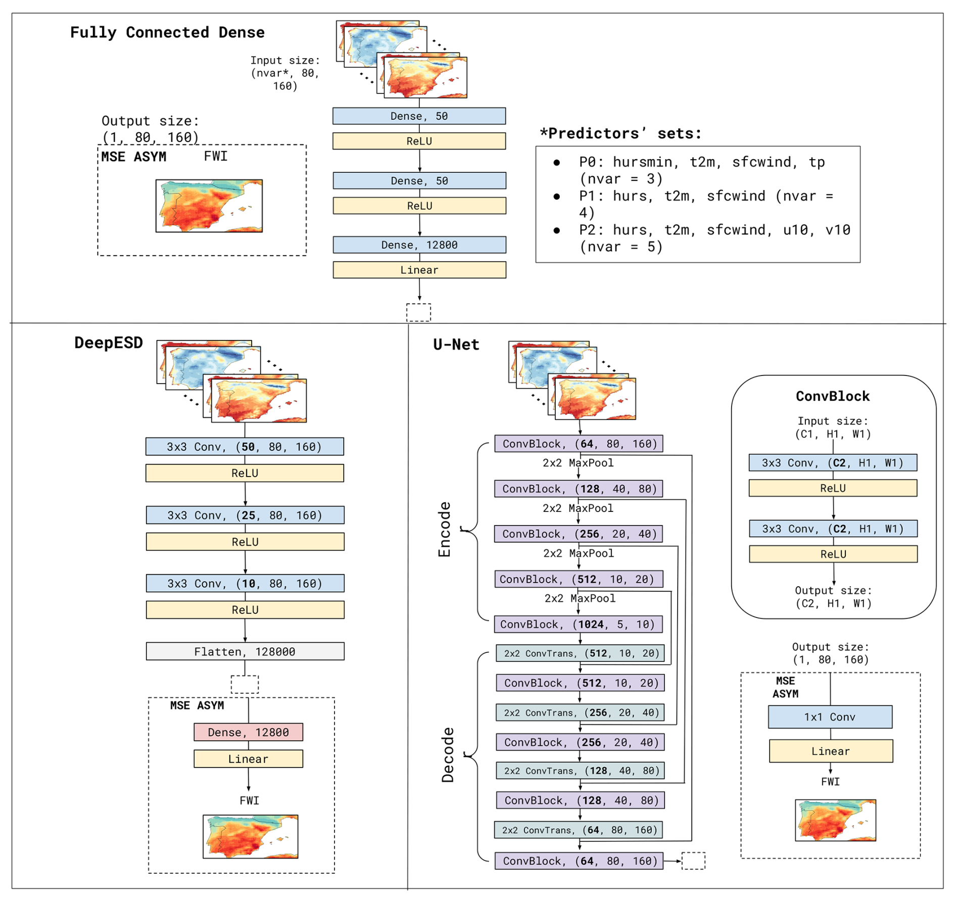
Figure 1 Schematic representation of the DL architectures used in this study, showcasing the different types of layers and their corresponding dimensions. The figure also highlights the distinct sets of predictors used as training inputs.

2.4.1 Fully Connected Dense

The Fully Connected Dense (FCD) model is a DL architecture that relies exclusively on fully connected layers to process spatial input data. The input is first passed through two consecutive dense layers, each containing 50 neurons, with Rectified Linear Unit (ReLU) activation functions (Glorot and Bengio, 2010) applied to introduce non-linearity and enhance feature extraction. Following these hidden layers, the transformed feature representation is fed into a fully connected layer with 12 800 neurons, utilizing a linear activation function to produce the final output. This output is then reshaped to match the dimensions of the predictand, ensuring consistency with the target variable.

2.4.2 DeepESD

The DeepESD model (Baño-Medina et al., 2022) is designed as a combination of convolutional and dense layers envisaged to efficiently process spatial data. It consists of three convolutional layers with 50, 25, and 10 kernels, each using ReLU activation functions (Fig. 1 for more details). After the final convolutional operation, the resulting feature maps are flattened into a one-dimensional vector, which is subsequently passed through a fully connected dense layer comprising 12 800 neurons, reshaping to match the dimensions of the predictand.

2.4.3 U-Net

The U-Net model adopts an encoder-decoder architecture designed for spatial data processing. The encoder progressively extracts hierarchical features through a series of Convolutional Blocks (ConvBlocks), each containing convolutional layers with ReLU activation, followed by 2×2 max pooling operations that reduce spatial dimensions while increasing the number of feature maps. The encoder expands from 64 to 512 channels, while reducing the spatial resolution from (80, 160) to (10, 20). In the decoder, the model reconstructs the original resolution using 2×2 transposed convolutions (deconvolutions) that progressively upsample feature maps (Prince, 2023). This is followed by convolutional layers that refine the output. The final layer consists of a 1×1 convolution, followed by a linear activation function, producing an output of dimensions (1, 80, 160).

2.4.4 Loss functions

The DL models were fitted with two alternative loss functions: the mean squared error (MSE), which serves as a standard loss function, and an asymmetric loss function (ASYM), designed to better capture extreme events, as introduced by Doury et al. (2024). The MSE is defined as the average of the squared differences between observed and predicted values. This metric penalizes larger errors more severely, making it useful for many regression tasks. However, MSE might not adequately emphasize errors associated with extreme events. To address this limitation, we implemented an asymmetric loss function defined as:

$$\begin{array}{}\text{(2)}& L_{\mathit{\theta }}={\displaystyle \frac{\mathrm{1}}{N}}\sum _{i=\mathrm{1}}^N|y_i-{\widehat{y}}_i|+{\mathit{\gamma }}^{\mathrm{2}}\times \max \left(\mathrm{0},y_i-{\widehat{y}}_i\right)\end{array}$$

where γ=G(y), where G is the gamma cumulative distribution function (CDF) fitted to the time series of every grid point in the training dataset. This loss function weights the mean absolute error (MAE) by an amount proportional to the extremity of each value, thus assigning a higher penalty when the model underestimates extreme values. This tailored approach improves the evaluation and prediction of extreme events in the dataset.

2.5 Model evaluation

In this study, the DL models are trained using daily data from the period 1979 to 2017. To evaluate the performance of the model, 20 % of these data is separated and treated as validation samples for model assessment during the training phase. The final results are presented for an independent test period spanning 2018–2021. We also evaluated longer test periods (2012–2021), which required shortening the training phase to 1979–2011. Since these tests produced robust and consistent results comparable to those for 2018–2021, they are not included in the text. To assess the performance of the DL models and the reproducibility of spatial and temporal patterns in the emulated results, several validation indices are used, each focusing on different spatial and temporal aspects of the predicted series (Table 2).

Table 2 Validation indices assessed in the study.

At each grid point, validation indices are computed, and their spatial distributions are depicted in the maps presented in various figures in Sect. 3. These indices span different key characteristics of the predicted series to assess how models emulate FWI, such as the mean FWI and extreme FWI distribution, or the length of spells for extreme FWI events. Instead of using MAE (for FWI and FWI95) or bias (for Max Spell95), we assess relative bias with respect to the frequency of FWI95, given by the following formula:

$$\begin{array}{}\text{(3)}& \text{Relative bias}={\displaystyle \frac{X-\widehat{X}}{X}}\times \mathrm{100}\end{array}$$

where X represents the observed and $\widehat{X}$ the estimated value.

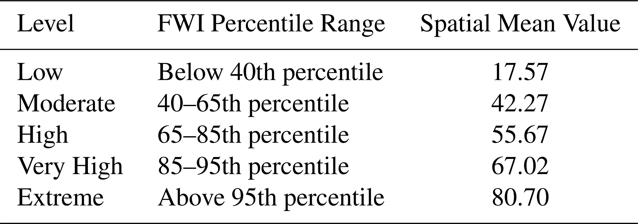
We also analyze the Receiver Operating Characteristic (ROC) curve, and the area Under the Curve (AUC), a graphical tool for evaluating the performance of binary classification models (Hogan and Mason, 2011), in this case applied to assess the DL model's ability to discriminate dangerous FWI events. It plots the true positive rate (sensitivity) against the false positive rate at various decision thresholds and quantifies the overall discriminative ability of the model, with values ranging from 0.5 (random classification) to 1.0 (perfect classification). A higher AUC indicates better model performance in distinguishing between positive and negative cases, making the ROC AUC particularly useful in unbalanced classification problems where traditional accuracy measures may be misleading. In particular, the classification evaluated in the ROC AUC analysis pertains to FWI events classified as “extreme” (see Table 3), defined as those exceeding the 95th percentile of the reference FWI, according to the danger levels established by the Spanish Meteorological Agency (AEMET, https://www.aemet.es/documentos/es/datos_abiertos/Estadisticas/IM_riesgo_incendios/eimri_generalidades.pdf, last access: 17 February 2025), being thus impact-relevant for wildfire risk assessment in the Iberian Peninsula. In addition to the validation indices listed in Table 2, we also use scatter plots the assessment of the emulated FWI 95th percentile against reference FWI climatologies, where the R² coefficient of determination is used.

Table 3 FWI Classes According to AEMET (Based on Percentiles). The right column shows the FWI reference spatial mean per category during the fire season.

2.6 Model explainability

DL models have demonstrated remarkable predictive capabilities across various scientific fields, yet their complex architectures often limit interpretability. This challenge has motivated the growth of eXplainable Artificial Intelligence (XAI), which aims to provide tools for understanding the underlying relationships learned by machine learning models (McGovern et al., 2019). In this work, we apply saliency-based methods to investigate the internal logic behind our DL predictions. Specifically, we employ a variant of the Integrated Gradients (IG) technique (Sundararajan et al., 2017), which has been widely adopted in climate applications (González-Abad et al., 2023; Kondylatos et al., 2022) for its effectiveness and ease of interpretability.

Traditional IG computes feature attributions by integrating the gradients of the model output with respect to the input, along a linear path from a baseline input to the actual input. The method is formally expressed as:

$$\begin{array}{}\text{(4)}& s_i(x_i;x_{\mathrm{b}})=(x_i-x_{\mathrm{b}})\underset{\mathrm{0}}{\overset{\mathrm{1}}{\int }}{\displaystyle \frac{\partial f\left(x_{\mathrm{b}}+t(x_i-x_{\mathrm{b}})\right)}{\partial x_i}}\mathrm{d}t\end{array}$$

where x_i is the feature value, x_b is the baseline (typically zero), and f is the output of the model.

However, in this study we adopt a simplified approximation of IGs, where the integral is omitted and the feature relevance is estimated directly from the gradients at the input point. This results in a computationally simpler, yet informative, saliency map representation. The relevance of each input feature is therefore computed as:

$$\begin{array}{}\text{(5)}& s_i\left(x_i\right)=x_i\cdot {\displaystyle \frac{\partial f\left(x\right)}{\partial x_i}}\end{array}$$

This approach preserves the core idea of attributing the prediction to the input features based on the local sensitivity of the model, while avoiding the computational overhead of path integration. Although this approximation does not fully satisfy all axioms of the original IG method (Sundararajan et al., 2017), it has been shown to yield stable and interpretable attributions in practical applications (Toms et al., 2021).

To address known XAI challenges (Mamalakis et al., 2023), the raw saliency maps are post-processed by: (1) taking the absolute value to focus on magnitude only, (2) zeroing all values below 10 % of the per-sample maximum to suppress gradient noise (Toms et al., 2021), and (3) normalizing each map so its values sum to one, thus yielding relative contributions. These normalized maps are used for all subsequent explainability analyses.

This methodology enables us to quantify the relative importance of each predictor variable in the model’s decision-making process, providing valuable insights into the learned relationships and the adequacy of the different sets of predictors tested, aiding in the underlying physical interpretation of the results.

2.7 Software

Both FWI calculation and emulation are carried out using the R-based climate4R framework (Iturbide et al., 2019). In particular, neural network emulators (Dense, DeepESD, U-Net) are defined and trained using the downscaleR.keras package (Baño-Medina et al., 2022), an extension of the downscaleR package (Bedia et al., 2020) that leverages Keras/TensorFlow.

3 Results and Discussion

Several DL models are evaluated through an intercomparison of different predictor sets (Table 1) and the loss functions optimized during DL model training (Sect. 2.4.4). The results presented in this section focus on the main fire season over the Iberian Peninsula (June to September, JJAS; see e.g. Bedia et al., 2014a) for the test period 2018–2021.

3.1 Proxy FWI validation

Figure 2 presents a multi-panel visualization, where the rows correspond to the validation measures shown in Table 2. From left to right, the first two columns represent the reference FWI and the Proxy FWI climatologies (P0, Table 1). The last column indicates the MAE or bias between both – depending on the evaluated index, Table 2–. The FWI95 frequency for the reference FWI is not shown, because, by construction, each grid point in the reference data records exactly 5 % of days above its local 95th percentile threshold during the season. Therefore, the value in each grid across the spatial map is 0.05. It serves as the observed reference for error calculation: The 95th percentile of reference FWI is used as baseline to compute the frequency of Proxy FWI events exceeding this threshold (as well as emulated FWI in the following section).

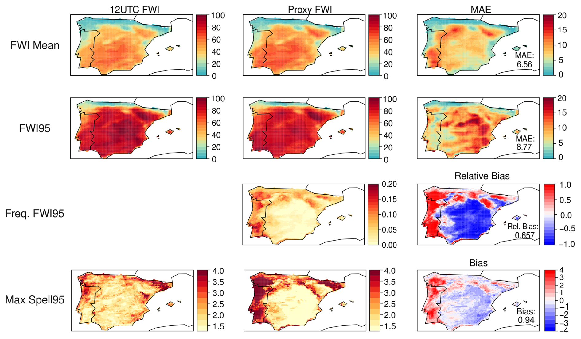
Figure 2 Reference and Proxy Fire Weather Index (FWI) climatologies for the fire season (June–September) during the test period (2018–2021). These include mean FWI, 95th percentile of FWI (FWI95), FWI95 frequency (number of days exceeding the reference FWI95) and the mean maximum annual spell (the number of days exceeding reference FWI95 Max Spell95). The third column displays the mean absolute error (MAE) for the FWI Mean and FWI95, the bias for Max Spell95 and the relative bias for the FWI95 frequency. The spatial averaged values of MAE or absolute (relative) bias are displayed at the bottom right.

Focusing on the differences between the Proxy and the reference FWI, we note that there exists greater MAE in Southern Portugal, North-western Spain and North-Eastern Spain, along the Ebro Valley. Conversely, the lowest MAE values (close to zero) are found along the Cantabrian and Mediterranean coasts, northwestern Portugal, the Pyrenees, and the Balearic Islands. These low-MAE areas generally align with the lowest climatological FWI values (as depicted in first column, first row), except for the Balearic Islands, where climatological JJAS FWI remains relatively high (FWI ≈ 35).

Regarding extreme FWI events (above reference FWI 95th percentile, FWI95), the Proxy FWI95 exhibits the highest MAE in the central-eastern and southeastern continental regions, coincident with very high reference FWI95 climatological values. Although the Proxy FWI95 accurately represents southern Portugal, revealing low MAE values, overall, the most critical FWI95 regions (mostly over Coastal Mediterranean and Central and Iberian Massifs) tend to be underrepresented by the Proxy FWI.

The Proxy FWI exhibits a relatively high bias in the frequency of FWI95 events, over continental and coastal Mediterranean regions (negative) as well as the western atlantic façade (positive). This behavior arises from structural differences between the Proxy formulation (based on daily aggregated variables) and the reference FWI, which depends on instantaneous noon-LST conditions. Because extreme fire-weather situations typically occur near midday, the use of daily means and daily minimum/maximum values smooths the sharp sub-daily variations that drive threshold exceedances, leading to systematic over- or under-counting of FWI95 days. Despite this limitation, the Proxy FWI reproduces the main spatial gradients and climatological patterns of mean FWI, FWI95 and Max Spell95, confirming that it remains a useful and physically consistent baseline against which to assess the added value of the deep-learning emulators. Regarding the temporal sequence of extreme–event occurrences, the relative bias for the FWI95 frequency displays a spatial pattern similar to that of the Max Spell95, with overestimation of FWI95 days in Portugal, north–western Spain (Galicia), the Cantabrian mountain range, the Pyrenees and the Ebro Valley, and substantial underestimation across the rest of the Iberian Peninsula. Consistently, the spatial distribution of Max Spell95 shows that the Proxy FWI overestimates spell lengths in Galicia and Portugal (by up to 4 d) while in the continental interior it tends to underestimate them, remaining close to the reference values over most of south–western Spain.

3.2 Emulated FWI validation

This section presents an intercomparison of the different DL models tested, by evaluating errors relative to the reference FWI and comparing them with the Proxy FWI results described in the previous section, which serves as a benchmark. For brevity, here we present the results using the predictor set P0 as input (Table 1), considering that the overall intercomparison results are consistent regardless of the predictor set tested. Since P0 includes the variables necessary for computing the Proxy FWI using the standard FWI formulation, our goal is to assess whether different DL architectures are able to capture the reference FWI more accurately using the same input information.

3.2.1 Prediction errors

The prediction errors for the Dense, DeepESD, and U-Net models relative to the reference FWI are presented in Fig. 3. The columns correspond to the results of each DL model, and the rows display various validation metrics, including the mean absolute error (MAE) for FWI and FWI95 or the relative bias in the frequency of FWI95. Below the error maps, a scatter plot is displayed per DL model, including the Proxy FWI, comparing the predicted climatological values against the reference FWI95.

Before discussing the performance of the DL models across the validation indices, we first highlight how daily aggregation of the input data affects model performance. Figure D1 in Appendix D presents the results from the Dense, DeepESD, and U-Net models trained using 12:00 UTC input variables (temperature, 24 h accumulated precipitation, relative humidity, and wind speed) to compute the FWI. This sensitivity experiment evaluates the models’ ability to learn the transfer function defining the FWI using inputs at 12:00 UTC, consistent with the temporal resolution of the reference index. This analysis complements our other model configurations by isolating the effect of temporal aggregation. Specifically, we compare performance when models are trained with instantaneous inputs (i.e., values at 12:00 UTC and 24 h precipitation) versus daily mean inputs. This framework allows us to separate the intrinsic biases of each model from the additional error introduced by using daily-aggregated predictors. Figure D1 shows that models trained with instantaneous inputs exhibit lower bias and improved accuracy while maintaining a similar spatial error pattern. This confirms that part of the error observed in experiment P0 (Fig. 3) stems from the mismatch in temporal resolution between the predictors and the reference FWI. However, some regions such as the Mediterranean areas for FWI MAE and the Cantabrian Mountains, the Pyrenees, and the Mediterranean coast for FWI MAE95 exhibit intrinsic errors even when instantaneous inputs are provided to the DL models. Moreover, the U-Net architecture demonstrates the lowest intrinsic bias in emulating the actual FWI function. It consistently shows the smallest biases in FWI and FWI95, as well as in the predicted frequency of FWI95 events and the mean annual maximum duration of FWI95 spells. These results suggest that U-Net offers enhanced generalization capabilities. Its ability to maintain low bias across both instantaneous and aggregated inputs indicates robustness to temporal variability, a key factor in modeling climate indices.

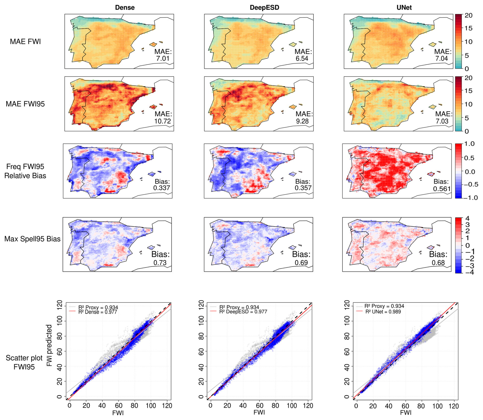
Figure 3 DL model results for various spatial validation indices presented in Fig. 2. The results depict the differences relative to the reference FWI for the fire season (June–September) during the test period (2018–2021). The scatter plots compare climatology values between the Proxy FWI95 (in grey) and the corresponding DL model predictions (in blue), against reference FWI95. Linear fits are shown in grey for the Proxy FWI95 and in red for the DL model, with the corresponding R² values displayed in the top-left corner.

Focusing on the intercomparison of DL models trained with P0, all DL models exhibit similar performance across the validation indices compared to the Proxy FWI output. For each validation index, at least one DL model outperforms the Proxy FWI. While Dense reveals slightly worst mean FWI MAEs (Fig. 3) than the Proxy FWI (Fig. 2), DeepESD and U-Net have comparable performance (6.54 and 6.01 vs. 6.56). However, the DL models provide a smoother spatial distribution of MAE across both continental and coastal Mediterranean regions. In contrast, as discussed in Sect. 2.2, the Proxy FWI exhibits large MAE values in FWI-prone areas, such as the Ebro Valley, the Cantabrian mountain range, and southern Portugal (Fig. 2), which are largely reduced by the DL emulated FWI (Fig. 3).

Regarding FWI95 MAE, the U-Net model improves upon the Proxy FWI results (8.19 vs. 8.77), offering a smoother MAE distribution across the region and particularly low MAE values in some continental areas in Spain, where the Proxy FWI exhibits large errors. Except for Portugal, the Cantabrian and the Mediterranean coast, the U-Net model outperforms the Proxy FWI across Iberia. Meanwhile, the other DL models display considerable MAE values, especially in central and northeastern Portugal and the Cantabrian mountain range, where these errors are larger than those of the Proxy FWI.

For FWI95 frequency, all three DL models outperform the Proxy FWI, with the U-Net model achieving the lowest relative bias. The Dense and DeepESD models generally underestimate FWI95 frequency across the region, except in southeastern Iberia and some localized areas in northern Iberia. Moreover, the U-Net model performs slightly better than the other DL models, overestimating FWI95 frequency across northern Iberia.

To assess the temporal characteristics of the emulated FWI, we evaluate Max Spell95 w.r.t. reference FWI. Here, the U-Net model achieves the best average result, closely followed by DeepESD (bias of 0.64 vs. 0.69). The key difference between these models is that U-Net generally overestimates is some northern areas, with maximum exceedances of 1–2 d, whereas DeepESD tends to overestimate, with discrepancies of up to 1–2 d in specific areas across the south-western of the Iberian Peninsula.

Despite these local problems, overall the scatter plots depict that DL models consistently improve upon the Proxy FWI results, regardless of the specific DL model. In terms of R², the U-Net model achieves the best performance for FWI95, with a value of 0.982, compared to 0.934 for the Proxy FWI. Overall in the FWI95 scatter plots, the Proxy FWI underestimates higher values (above 60 for the reference FWI95), while the U-Net model, in particular, offers a significantly better representation of reference FWI.

Furthermore in Fig. 4, we assess the DL model ability in discriminating extreme fire danger events (i.e., reference FWI values above the 95th percentile) using ROC-AUC histograms, where the Proxy FWI is represented in red and the DL models in blue. Overall, the DL models improve upon the results provided by the Proxy FWI. Regarding extreme event detection, DeepESD demonstrates the best performance, with a median ROC-AUC of 0.734, compared to 0.727 for U-Net and 0.7 for the Dense model, as shown in the histograms (Fig. 4). In this regard, the DL models outperform the Proxy FWI, as indicated by the higher frequency of ROC-AUC values above 0.5 (indicating better-than-random classification). The only exception occurs for ROC-AUC values above 0.9, which correspond to the classification of grid points along the Cantabrian coast, where climatological FWI is the lowest Iberia (Fig. 2) due to generally milder and moist conditions throughout the year, where Proxy FWI exhibits better FWI95 event discrimination than DL models.

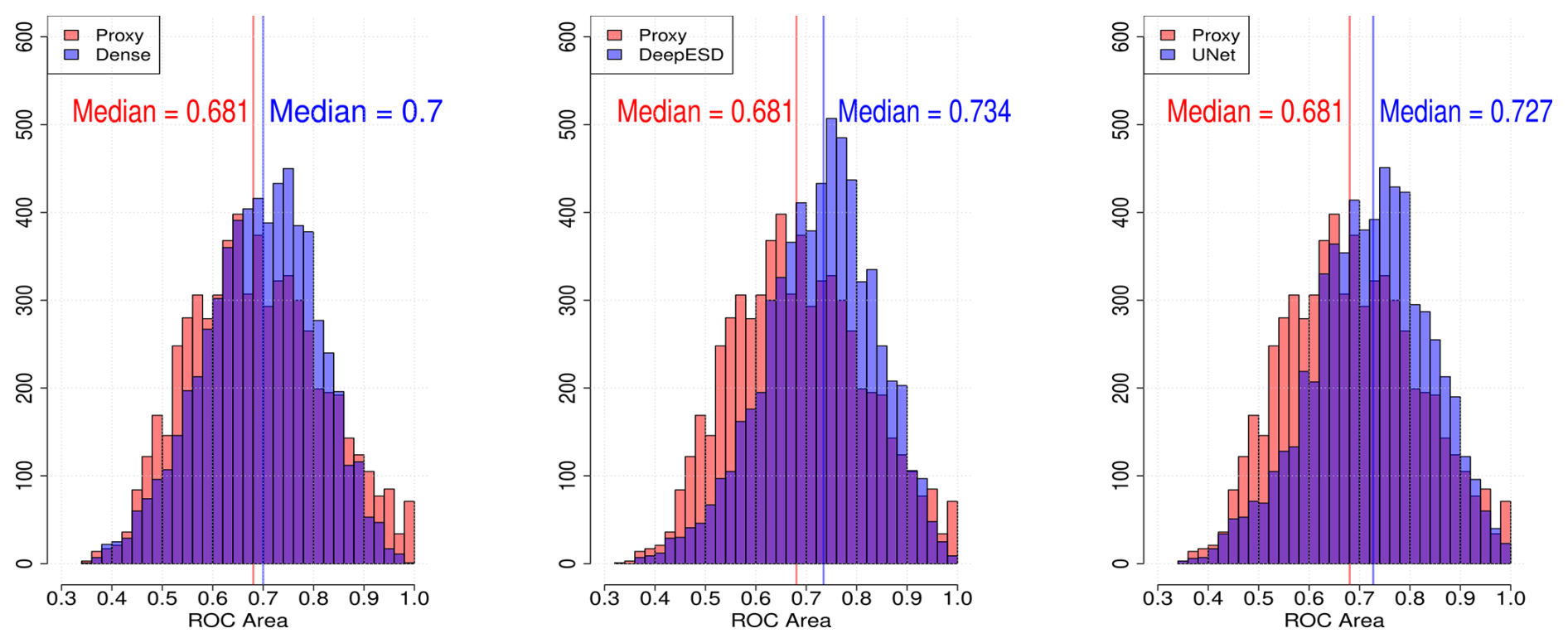
Figure 4 DL prediction results corresponding to the fire season (June–September) for the test period (2018–2021). Histograms compare the Area Under the ROC Curve (AUC)for extreme FWI event classification (above the 95th percentile) at each grid point, between the Proxy FWI (in red) and the corresponding DL model (in blue). The median values of both are also indicated.

In addition to the spatial assessment, we provide an analysis of the monthly boxplots of the Reference FWI, Proxy FWI, and the DL-predicted FWI (Dense, DeepESD, and U-Net) for each climatological region, as shown in Fig. 5. Each boxplot represents the distribution of FWI values for a given month over the 2018–2021 period, capturing both the median and the spread of the values across the climatological regions (ATL, COASM, and CONTM; see Fig. 2). This visualization demonstrates that the DL models not only reproduce the spatial patterns of FWI but also effectively capture the temporal variability across the year and across different regions. The median and interquartile ranges of the DL predictions closely follow the Reference FWI throughout the seasonal cycle, including the high-risk summer months, whereas the traditional Proxy FWI tends to underestimate extremes during peak months (June–September). The results further show that the Proxy FWI departs from the reference, particularly during the summer when values are highest and variability is greatest. In contrast, the DL models consistently produce distributions that are much closer to the Reference FWI, reducing the discrepancies observed with the proxy. This improvement is shown in all three regions, confirming that the advantage of the DL models over the Proxy FWI is robust and not region-specific. The closer alignment of the DL predictions with the reference highlights their capacity to more accurately capture the seasonal dynamics of fire weather conditions without introducing significant seasonal biases.

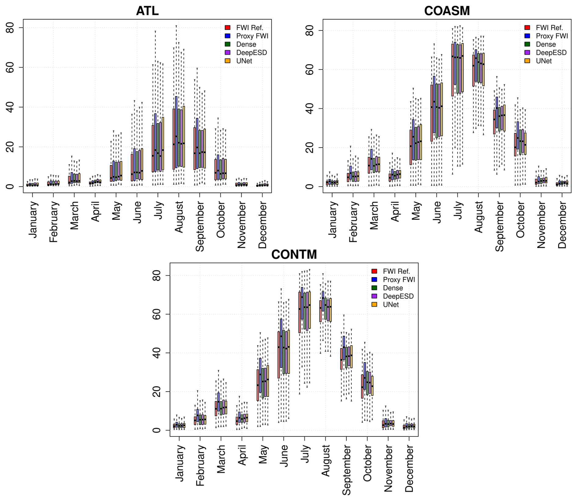
Figure 5 Monthly boxplots for the reference FWI, proxy FWI, and the DL-predicted FWI (Dense, DeepESD, UNet) for CONTM (top-left), COASM (top-right) and ATL (bottom) regions. Each boxplot represents the distribution of FWI values for a given month over the test period, capturing both the median and the spread of the values.

3.3 Emulation Model Explainability

Here, we analyze the saliency attributed to the predictor variables, grouped by the same climatic regions and fire danger categories defined in Appendix A. The overall results indicate no major differences in the saliencies of the different DL models, underpinning their robustness and physical coherence. Therefore, here we present the explainability results of the U-Net model, since it outperforms Proxy FWI and attains similar validation results as DeepESD, while offering greater computational efficiency. To this aim, we compute the saliencies of each variable considering the time events corresponding to the different fire danger categories separately (Fig. 6).

Focusing on the high, very high, and extreme fire danger categories, temperature and relative humidity emerge as the most influential variables in the model’s predictions. The relative importance of these two variables varies across climatic regions. In the Continental Mediterranean region, temperature and relative humidity show similar levels of saliency. For the high fire danger category, relative humidity slightly surpasses temperature, whereas for the very high and extreme categories, temperature becomes more dominant. Wind speed consistently ranks as the third most important variable in these categories, although its relevance diminishes as the fire danger increases. The relatively low saliency of wind speed for the most severe categories reflects both the structure of the training data and the role that wind plays within the Fire Weather Index (FWI) formulation at very high danger levels. In Iberia, extreme fire danger episodes are predominantly associated with persistent heat anomalies, very low relative humidity, and sustained fuel desiccation, rather than with short-lived wind maxima. Once fuels are critically dry, additional increases in wind speed exert a comparatively smaller influence on the final FWI class than thermodynamic controls, which leads the model to rely more strongly on temperature and relative humidity when discriminating between extreme and very extreme conditions. Moreover, wind exhibits higher temporal variability and weaker spatial coherence than the other predictors, particularly when daily aggregated inputs are considered.

This finding is consistent with the definition of the FWI itself, which relies primarily on temperature, relative humidity, and wind speed under dry conditions. The DL model thus reflects the structure and sensitivity of the FWI metric it is trained to emulate. Importantly, this does not mean that precipitation (or other inputs) is irrelevant for real-world fire risk; rather, it highlights that the predictand (FWI) gives limited weight to precipitation in high and extreme danger situations. Moreover, ERA5-Land predictor variables are not independent. Relative humidity, for instance, is derived from temperature and dew point, which are indirectly influenced by precipitation, while precipitation and wind are assimilated forcings. These inter-dependencies likely contribute to the model’s ability to achieve high predictive accuracy even when precipitation and wind receive lower attribution scores.

The Coastal Mediterranean region shows a similar pattern. However, in the high category, temperature becomes more salient than relative humidity. In contrast, for the extreme category, relative humidity overtakes temperature as the most relevant predictor.

Similarly, in the Atlantic region, temperature is the most significant variable for the high and very high categories. For the extreme category, however, relative humidity surpasses temperature. Notably, in this region, the difference in saliency between wind speed and the top-ranked variables is smaller compared to other regions, suggesting a higher reliance on this variable in this region. As with the other regions, the relevance of wind speed decreases with increasing fire danger, and precipitation remains consistently negligible.

For the medium and low fire danger categories, the importance of variables shifts more markedly and shows less consistency across climatic regions. In the Continental and Coastal Mediterranean regions, precipitation becomes the most relevant variable for the low category, followed by relative humidity, wind speed, and temperature. For the medium category, wind speed emerges as the most salient predictor, followed by temperature, relative humidity, and precipitation.

In contrast, in the Atlantic region, relative humidity is the most important variable for the low category, followed by precipitation, wind speed, and temperature. For the medium category, temperature takes the lead, followed by wind speed, relative humidity, and finally precipitation. These results suggest that precipitation is a key variable for low fire danger levels but loses significance as fire danger increases, becoming practically irrelevant in extreme conditions, when temperature and relative humidity gain prominence and become the most critical predictors. This is consistent with numerous studies that highlight the importance of high temperatures and low humidity in contributing to extreme fire danger (Jain et al., 2022).

Given that precipitation has negligible saliency in high percentile fire danger cases, which are precisely the most important from the point of view of impacts, the next section evaluates model performance after removing precipitation from the predictor set. We also examine alternative predictor sets, including replacements for precipitation and wind speed, such as eastward and northward wind components, under the hypothesis that these may carry additional useful information for the emulators.

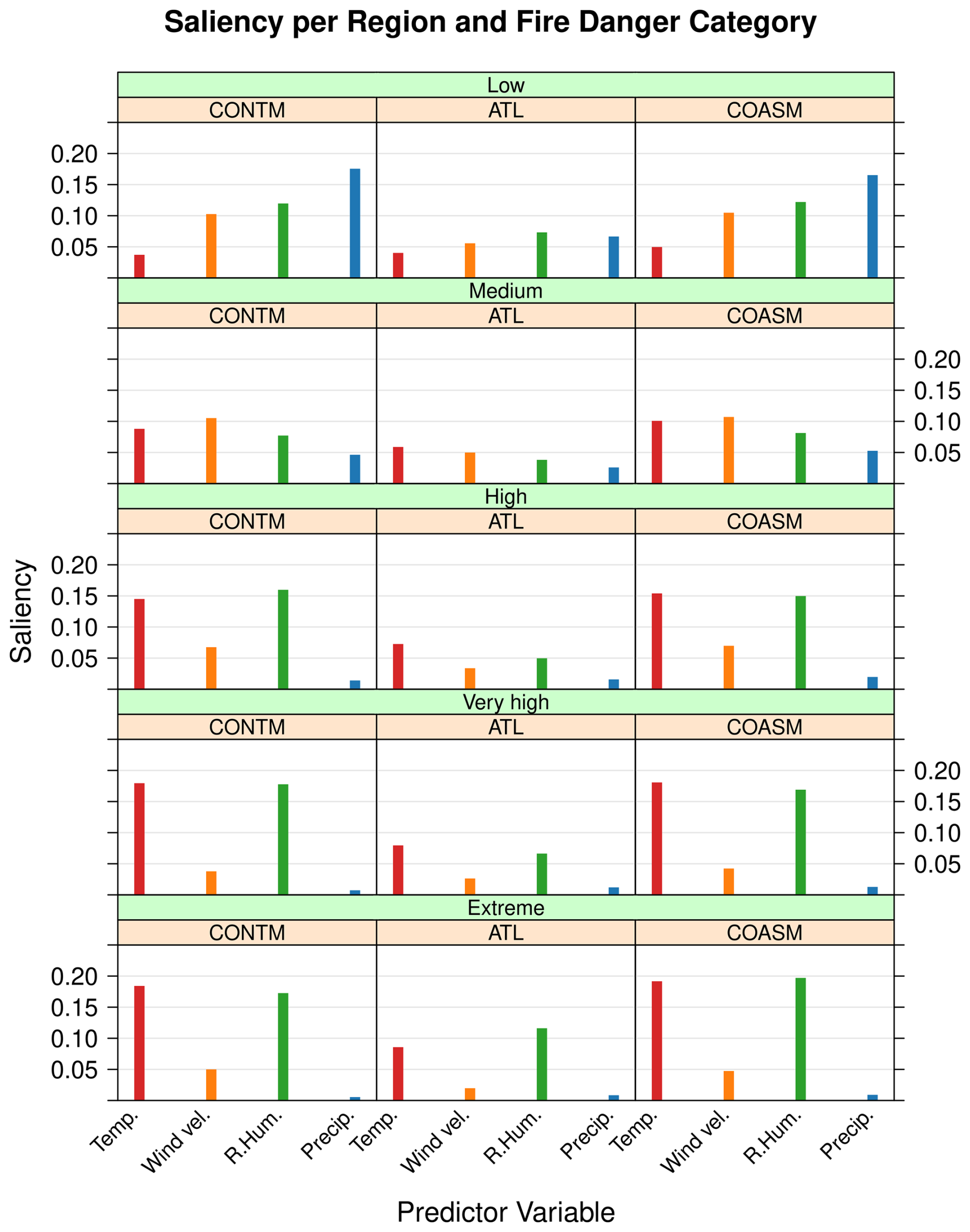
Figure 6 Aggregated saliency of predictor variables by climatic region and fire danger category for the U-Net model. Columns represent the climatic regions defined in Fig. A1, while rows correspond to the fire danger categories described in Sect. 3.2. The displayed saliency values are derived from saliency maps, normalized at each grid point. Results for the JJAS season, test period (2018–2021).

3.4 Predictor set intercomparison

In this section, we intercompare different alternative input predictor sets, summarized in Table 1. For simplicity, we focus on the U-Net DL method as in Sect. 3.3. The U-Net trained with P0 and P1 yields better results than when trained with P2, except for the MAE FWI (Fig. 7, analogous to Fig. 3 for comparability). The difference between U-Net P0, U-Net P1 and U-Net P2 is relatively small, with the most remarkable variations observed in the western Continental region. For the MAE of FWI95 events, U-Net P2 significantly overestimates across the entire domain, whereas U-Net P0 and U-Net P1 present similar MAE spatial distribution, standing P1 as the best approach. However, U-Net P1 shows a greater presence of errors in specific regions, such as north Portugal, the Pyrenees and the Cantabrian mountain ranges. Regarding the frequency of FWI95 events, U-Net P0 tends to overestimation across nearly the entire the north domain, while U-Net P1 tends to overestimate in the mid-south and east of the Peninsula and U-Net P2 exhibit a general underestimation. Among these, U-Net P0 appears to be the most effective in capturing this index. Examining the Max Spell95 results of the different experiments, U-Net P2 performs the worst, with overestimation up to 3 to 4 d in some areas, whereas the largest differences in P0 and P1 range between 2 and 3 d at most. U-Net P1 shows a slight improvement over U-Net P0, displaying more areas of overestimation, while U-Net P0 predominantly underestimates across most of the domain. Finally, the FWI95 scatter plots exhibit a high R² fit for all three predictor sets, outperforming the Proxy FWI. In terms of overall performance, U-Net P1 produces the best results, followed by U-Net P0 and U-Net P2, though the differences among the latter remain relatively small.

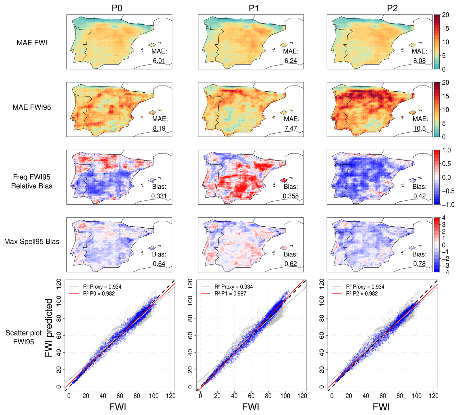
Figure 7 U-Net model results for various spatial validation indices presented in Fig. 2 and different predictors sets assessed (see Table 1). The results depict the differences relative to reference FWI for the fire season (June–September) during the test period (2018–2021). Additionally, scatter plots compare climatology values of the Proxy FWI95 (in grey) and the U-Net model (in blue) against reference FWI95. Linear regression fit lines are shown in grey for the Proxy FWI95 and in red for the U-Net model (to enhance visualization), and the corresponding R² values displayed in the top-left corner.

Overall, in Fig. 8, U-Net P1 yields the best results as classifiers for extreme events. These experiments improve upon the median results of the Proxy FWI, with U-Net P1 emerging as the most effective model in this context.

In summary, the U-Net model demonstrates superior performance over the Proxy FWI, with U-Net P1 generally excelling in overall performance. The inclusion of wind components as additional predictors in P2 has a deleterious effect on the temporal and distributional similarity of emulated and reference FWI. This suggests that, for emulating the FWI index itself, wind speed magnitude already captures the relevant wind-related information, and the addition of directional components introduces redundant or noisy predictors that can hamper model performance, despite the internal feature selection of deep learning methods. Consequently, a prior predictor screening may still be necessary to ensure optimal results. Importantly, as seen through the current section, the scope of this work is restricted to the statistical reconstruction and characterization of fire-weather conditions as represented by the FWI, rather than the analysis of wildfire occurrence, behavior, or impacts. The DL-based results are validated considering the FWI95, FWI95 frequency and the Max Spell95 (Figs. 3 and 4) and the AUC of the ROC curve for extreme fire danger classification as noted in Figs. 7 and 8. With this suite of validation metrics and experiments, we properly assess the ability of the DL-based results to statistically reproduce the most extreme events. Consequently, we do not investigate individual wildfire events or fuel-specific fire behavior, which lie outside the intended scope of this study.

3.5 Loss function assessment

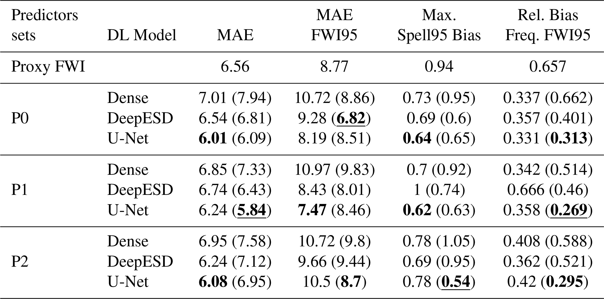
We next present a summary of the validation results, including an intercomparison of alternative MSE and asymmetric loss functions in the DL models (Sect. 2.4.4). Table 4 presents the validation indices for different predictor sets and DL models, comparing their performance against the Proxy FWI baseline, where the ASYM loss function values are indicated in parentheses. For all indices, the DL models exhibit consistent improvements over the Proxy FWI, with at least one model outperforming it in each category.

Regarding the loss function, the ASYM loss generally improves performance in most validation indices. The ASYM-trained models tend to yield lower MAE than ASYM values, particularly for DeepESD in P1 (6.74 vs. 6.43) and P2 (6.24 vs. 7.12), showing better accuracy in estimating FWI. Similarly, in the FWI95 MAE, the ASYM-trained models consistently outperform MSE loss counterparts, as seen with DeepESD in P0 (9.28 vs. 6.82) and P2 (9.66 vs. 9.44). In terms of extreme event prediction, the Max Spell95 Bias shows inconclusive results. While the ASYM loss function improves the bias in some cases, such as U-Net in P2 (0.78 vs. 0.54), in other cases, it worsens bias, as observed with Dense in P2 (0.78 vs. 1.05). This suggests that ASYM does not consistently improve the temporal persistence of extreme events but may still provide benefits in specific cases. For the Relative Bias Frequency of FWI95, ASYM provides substantial benefits in reducing bias. The most notable case is U-Net in P1, where the ASYM-trained model achieves a significantly lower bias (0.358 vs. 0.269) than MSE, reinforcing ASYM's ability to enhance the reliability of extreme event frequency estimations.

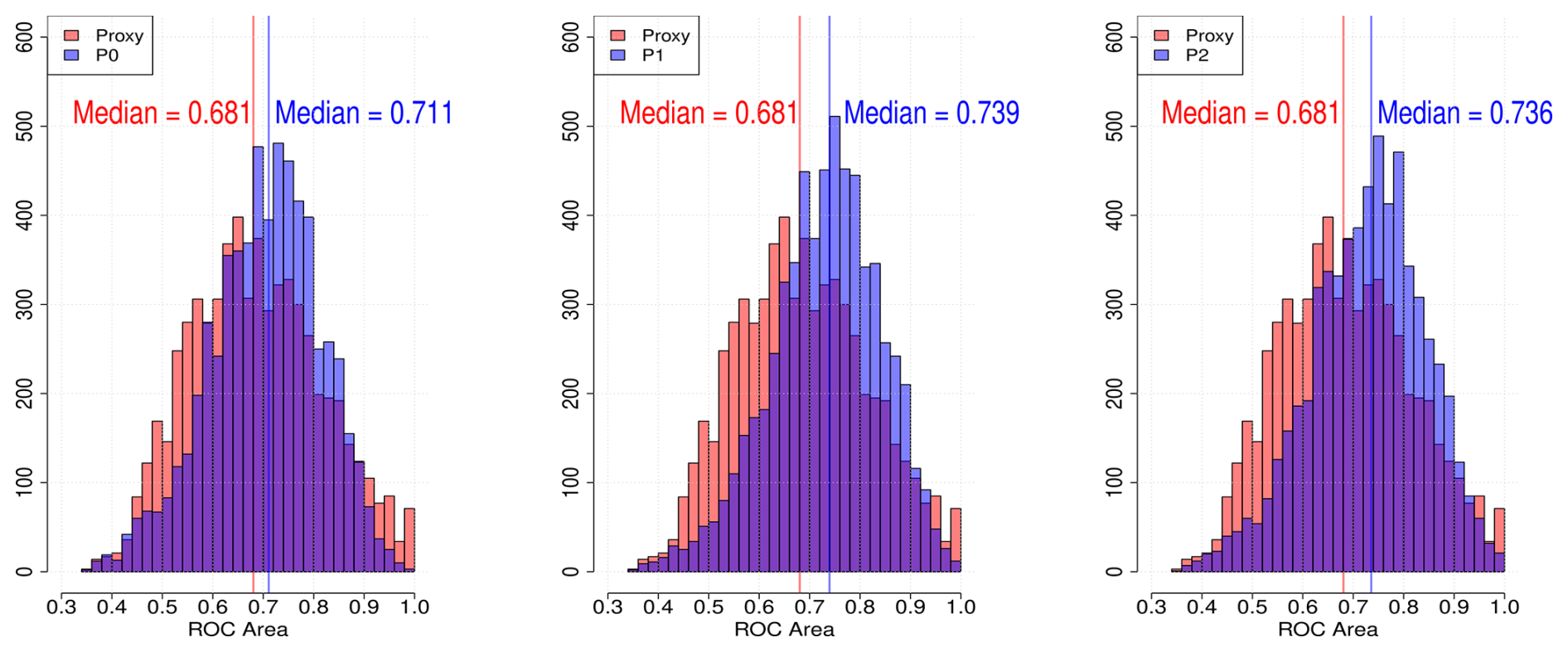
Figure 8 U-Net model histograms results for the fire season (June–September) for the test period (2018–2021). Histograms compare the Area Under the Curve (AUC) of the Receiver Operating Characteristic (ROC) curve for extreme fire danger classification (above the 95th percentile) at each grid point between the Proxy FWI (in red) and the U-Net model (in blue). The median value is indicated for both results.

Overall, ASYM appears to be particularly beneficial in reducing error in FWI estimations (MAE and MAE FWI95) and in improving the classification of extreme fire weather danger, as evidenced by the lower relative bias for FWI95 than MSE. However, its benefits on temporal aspects, such as Max Spell95 Bias, are not consistent. These findings suggest that while ASYM is generally advantageous, its effects are model- and index-dependent, although sometimes overestimates low and moderate values in the distribution (see Fig. C1). Therefore, the ASYM loss function does not compromise the U-Net model performance in the lower quantiles, however for the Dense and DeepESD models low and moderate values for the FWI are worse than using the MSE as loss function. Therefore, the ASYM loss function can compromise the performance of low and moderate levels in some cases, and its selection should be carefully considered depending on the primary objective of the analysis.

Table 4 Validation results of DL FWI emulators for different predictor sets. Values in parentheses are for the ASYM loss function for model training (default values correspond to MSE loss). The first row presents the Proxy FWI results, as benchmark. Bold values highlight the best validation index within each predictor set, while underlined values denote the overall best across all indices.

3.6 Fuel Moisture Code sub-indices Assessment

The Canadian Forest Fire Weather Index System is structured around six interrelated components that describe both fuel moisture conditions and potential fire behavior. In particular, the three fuel moisture codes Fine Fuel Moisture Code (FFMC), Duff Moisture Code (DMC) and Drought Code (DC) represent distinct organic layers with characteristic response times ranging from hours (surface litter) to months (deep compacted layers). These components provide physically interpretable proxies of ignition potential, fire sustainability and drought build-up, and they underpin the behavior of the aggregated FWI. Given their distinct physical meaning and temporal memory, assessing the performance of the deep-learning emulators at the level of the individual moisture codes provides an additional and more stringent evaluation of the modeling framework. To explicitly evaluate rainfall sensitivity and temporal memory across scales, two predictor configurations are considered: P0, which includes precipitation, and P1, which excludes it. This design enables a controlled assessment of the extent to which daily precipitation information contributes to the emulation of fast-, intermediate-, and slow-response fuel layers. Beyond reproducing the aggregated FWI, this analysis examines whether the emulators are able to capture the multi-scale fuel-moisture dynamics embedded in the structure of the system. We emphasize that this analysis should be regarded as preliminary, and that a more comprehensive and detailed assessment is currently under development. Nevertheless, the present evaluation provides an initial characterization of the performance of the DL model originally designed to emulate FWI when the predictand is replaced by its individual fuel moisture components (DC, DMC, or FFMC) instead of the aggregated FWI index.

Table 5 summaries the validation performance of the emulators for DC, DMC and FFMC under the two predictor configurations (P0, including precipitation; P1, excluding precipitation). The evaluation considers some of the validation metrics as the MAE, FWI95 MAE and relative bias in the frequency above the 95th percentile previously depicted in the manuscript. Moreover, we introduce an additional validation metric to explicitly assess the temporal consistency of the predicted subindex relative to the reference subindex. Specifically, we compute the Pearson correlation coefficient between the predicted and reference spatially aggregated time series. Prior to calculating the correlation, the seasonal cycle is removed from both time series to isolate anomalies and avoid inflating the correlation due to the shared annual cycle. To this end, the daily climatology (i.e., one value per Julian day of the year) is subtracted from each daily value in the time series. The daily climatological values are estimated over the full reference period using a centered moving average window of seven days, which smooths high-frequency noise while retaining the intra-seasonal structure of the climatology. This metric provides a domain-integrated measure of the emulator ability to reproduce the large-scale temporal variability of the fuel moisture codes, focusing explicitly on inter-daily to synoptic-scale fluctuations rather than on the mean seasonal evolution. As in the previous sections, these metrics are evaluated for the fire season (JJAS) in the test period (2018–2021), with the exception of the time series correlation, which is computed over the full annual cycle.

Table 5 Validation results of DL emulators for different predictor sets and FMC subindices; DC, DMC and FFMC.

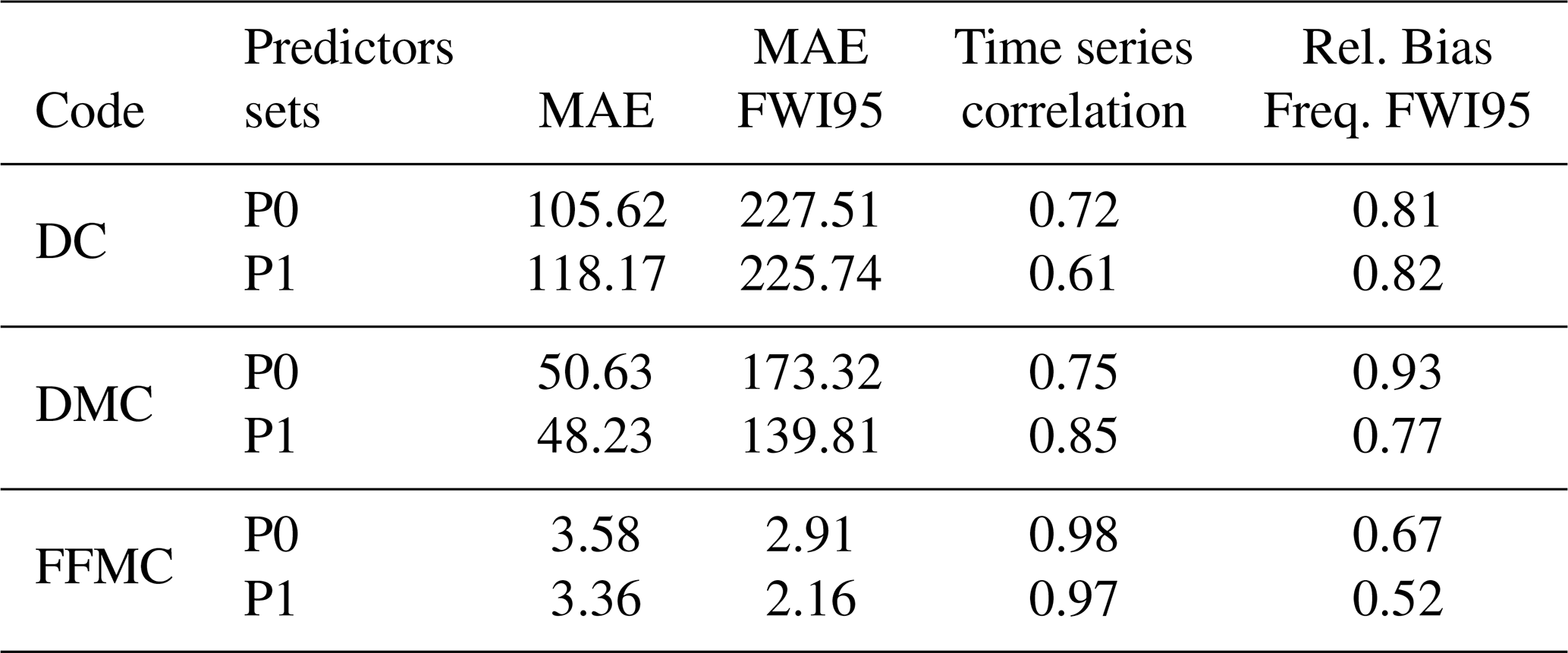
For the DC, which reflects long-term deep fuel moisture and cumulative drought effects, correlations are moderate (0.72 for P0 and 0.61 for P1). This suggests a greater challenge in fully capturing low-frequency variability and long-memory dynamics. Absolute errors are comparatively large in magnitude (MAE ∼ 106–118), which is consistent with the broader dynamic range of the DC. P0 achieves both lower MAE (105.62 vs. 118.17) and comparable performance under extreme conditions (FWI95: 227.51 vs. 225.74 are nearly identical, with a slight advantage for P1 in extremes but a higher overall MAE). The relative bias in high-danger frequency is very similar between predictor sets (0.81–0.82), indicating comparable representation of extreme drought-related conditions despite differences in correlation strength. The modest improvement obtained when precipitation is included is consistent with the DC formulation, where only substantial or sustained rainfall events effectively reduce deep-layer dryness; although such events are infrequent during JJAS, their accumulated impact contributes to improved interannual and low-frequency variability representation.

The temporal evolution shown in Fig. E1 provides additional context for interpreting the DC results. Despite the moderate correlations obtained for both predictor configurations, the DL reconstructions reproduce the main seasonal cycle and the timing of the major multi-month drought episodes throughout the 2018–2021 test period. Moreover, the two predictor sets generate remarkably similar DC trajectories, with only minor differences in amplitude and short-term fluctuations. This behavior is consistent with the validation metrics and indicates that the reduced skill observed for DC cannot be attributed solely to the exclusion of precipitation from the predictor set. Rather, it reflects the intrinsic difficulty of reproducing the long-memory dynamics and low-frequency variability embedded in the DC using architectures that do not explicitly model temporal dependencies, irrespective of whether precipitation is included. This limitation is further quantified in Appendix E, where the analysis of temporal persistence reveals a pronounced underestimation of memory for the DC. Together, these results demonstrate that the challenge lies primarily in the representation of persistence rather than in the availability of predictor variables. We note that this limitation is not intrinsic to the emulation framework itself, but to the specific class of architectures employed. Models explicitly designed to capture temporal dependencies, such as ConvLSTM networks, have been shown to better reproduce long-memory processes in a fire-weather prediction context (Mirones et al., 2025), albeit at a substantially higher computational cost, which limits their applicability in large-domain experiments such as the one presented here.

In the case of the DMC, representing intermediate-depth organic layers with response times of days to weeks, correlations are moderate to high (0.75 for P0 and 0.85 for P1). The removal of precipitation as a predictor in P1 markedly improves temporal correspondence. Overall MAE is slightly lower for P1 (48.23 vs. 50.63), and performance under extreme fire-weather conditions improves substantially (MAE FWI95: 139.81 vs. 173.32). The relative bias in high-danger frequency decreases from 0.93 (P0) to 0.77 (P1), indicating improved prediction of extreme-category occurrence under P1. This behavior indicates that during the Iberian fire season the DMC signal is largely governed by medium-term atmospheric drying driven by temperature and relative humidity, whereas rainfall events exceeding the effective infiltration threshold are comparatively rare at daily scale, thereby limiting the incremental value of explicit precipitation information for seasonal emulation.

Finally, for the FFMC, which governs short-term surface litter moisture and ignition potential, correlations are very high (0.98 for P0 and 0.97 for P1), demonstrating strong skill in reproducing rapid variability. Absolute errors are small (MAE ∼ 3.4–3.6; MAE FWI95: 2.16–2.91), with negligible differences in mean and extreme performance between predictor sets. The relative bias in extreme-day frequency decreases from 0.67 (P0) to 0.52 (P1), indicating improved representation of high-danger occurrences. Given the intrinsic sensitivity of FFMC to even light rainfall, the small differences between P0 and P1 suggest that the deep-learning architecture is able to reconstruct short-term surface moisture variability primarily from thermodynamic and wind predictors at daily scale, while the limited seasonal contribution of precipitation reflects its low frequency during JJAS rather than a lack of physical responsiveness.

In summary, the DL framework shows scale-dependent performance: very strong skill for the fast-response FFMC, moderate-to-high skill for the DMC (particularly under P1), and comparatively lower temporal fidelity for the slow-evolving DC. Despite these differences, biases in extreme-category frequency remain within a relatively narrow range, suggesting that the hierarchical structure of fuel-moisture dynamics is largely preserved. The differential sensitivity observed across predictor configurations is consistent with the physical formulation and temporal memory of each code, reinforcing the internal coherence of the emulation framework across fast, intermediate, and slow fuel-moisture regimes. Future work will also focus on the implementation of the emulator within the context of the PTI-Clima climate-service initiative (https://pti-clima.csic.es/, last access: 24 June 2026), alongside a more exhaustive validation against selected real-world wildfire events.

4 Conclusions

In this study we addressed the challenge of emulating the reference Canadian Fire Weather Index (FWI), which requires instantaneous noon meteorological inputs that are rarely available in observational databases or climate model output. We proposed a deep-learning framework capable of reconstructing the reference FWI from commonly available daily variables and evaluated its performance over the Iberian Peninsula. Our results show that (i) all emulators reproduce the main spatial and temporal characteristics of the reference FWI, including high-percentile behavior (critical for extreme fire danger detection); (ii) they consistently outperform the “traditional” Proxy FWI – as introduced by Bedia et al. (2014a) for regional climate projections–, particularly in the detection of extreme fire-weather events; (iii) daily mean predictors are sufficient to recover the reference FWI signal with high fidelity; (iv) the emulator can approximate the FWI with limited accuracy loss even when precipitation is omitted from the predictors, a result that likely reflects the model's ability to indirectly recover precipitation-related information through covariation with other meteorological variables (temperature, humidity, wind) and learned climatological patterns, rather than indicating that precipitation is physically unimportant for the FWI system; and (v) the U-Net and DeepESD architectures offer the best overall balance across metrics. These findings highlight the potential of DL-based emulators to provide accurate fire-weather information when sub-daily inputs are unavailable, and to circumvent data limitations in applications where certain predictors may be missing or uncertain.

A key methodological distinction should be emphasized for the proper interpretation of these results: the reference FWI is computed from instantaneous noon LST meteorological variables as originally defined in the FWI system, whereas the DL emulators are trained using daily-aggregated predictors (daily means, minima, or accumulated values). The reported emulator skill should therefore be understood as the ability of DL models to recover a noon-time fire-weather signal from daily-aggregated inputs, a practically valuable capability precisely because such inputs are far more widely available than instantaneous noon observations.

Placed in the context of previous work, our results address a well known problem with FWI reconstruction from model outputs (Herrera et al., 2013), that can also be circumvented through the use of FWI-derived indicators (e.g.: Matteo et al., 2025), posing a challenge in future climate impact studies and introducing additional uncertainty in the resulting projections. Our study extends earlier studies that relied on proxy variables to approximate the noon-LST FWI signal (Bedia et al., 2014a), demonstrating that DL methods can recover the nonlinear relationships between daily predictors and instantaneous fire-weather conditions more effectively than proxy formulations. This improvement is particularly relevant for Mediterranean-type climates, where strong diurnal cycles amplify mismatches between daily means and noon conditions, and for climate-change applications relying on coarse temporal resolution model output. The study does, however, have limitations. The emulators were trained solely on ERA5-Land, which is not an observational ground truth; also, for simplicity, the analysis is restricted to the generic JJAS fire season (although the simulations are performed for the entire period), even though the fire season period varies across ecoregions within the Iberian Peninsula (see e.g. Bedia et al., 2014b). Additionally, while the precipitation-free experiments demonstrate the emulator's robustness under the specific conditions of the JJAS season, the results should not be interpreted as evidence that precipitation is physically unimportant for the FWI system. Rather, this finding illustrates how deep learning models can leverage statistical relationships and learned representations to approximate indices in data-sparse contexts, which may be valuable for applications but does not diminish the fundamental role of precipitation in fire-weather dynamics. Finally, the emulators are sensitive to the spatiotemporal characteristics of the training dataset and may require adaptation in environments with different climatic regimes. Our preliminary experiments on the individual fuel-moisture codes (FFMC, DMC, DC) show that FFMC and DMC can be emulated accurately from daily inputs, while the DC exhibits a stronger sensitivity to long-term memory processes, which are more challenging to reproduce with architectures that do not explicitly model temporal dependencies. This limitation could be alleviated by architectures explicitly designed to capture temporal dependencies, although their application at large spatial scales remains computationally demanding (Mirones et al., 2025). As this study focuses on the FWI – the final, integrated index most widely used in climate and impact applications – we leave a full component-level assessment to a companion work. Future research should also assess the practical implications of emulator performance through analyses of specific wildfire episodes, evaluating how accurately reconstructed fire-weather conditions translate into the detection and characterization of documented fire events. Such event-based validation would provide a complementary perspective to the statistical evaluation presented here and help further establish the applicability of the proposed framework in impact-oriented contexts. Ongoing research is extending this framework to other regions and seasons, incorporating additional environmental predictors, and analyzing the physical behavior of the individual FWI components in greater depth.

Appendix A: Climatological regions

Here, we present the division of the Iberian Peninsula into three regions – Atlantic (ATL), Continental Mediterranean (CONTM), and Coastal Mediterranean (COASM) – for the eXplainable Artificial Intelligence (XAI) analysis provided in the main manuscript (Fig. 6).

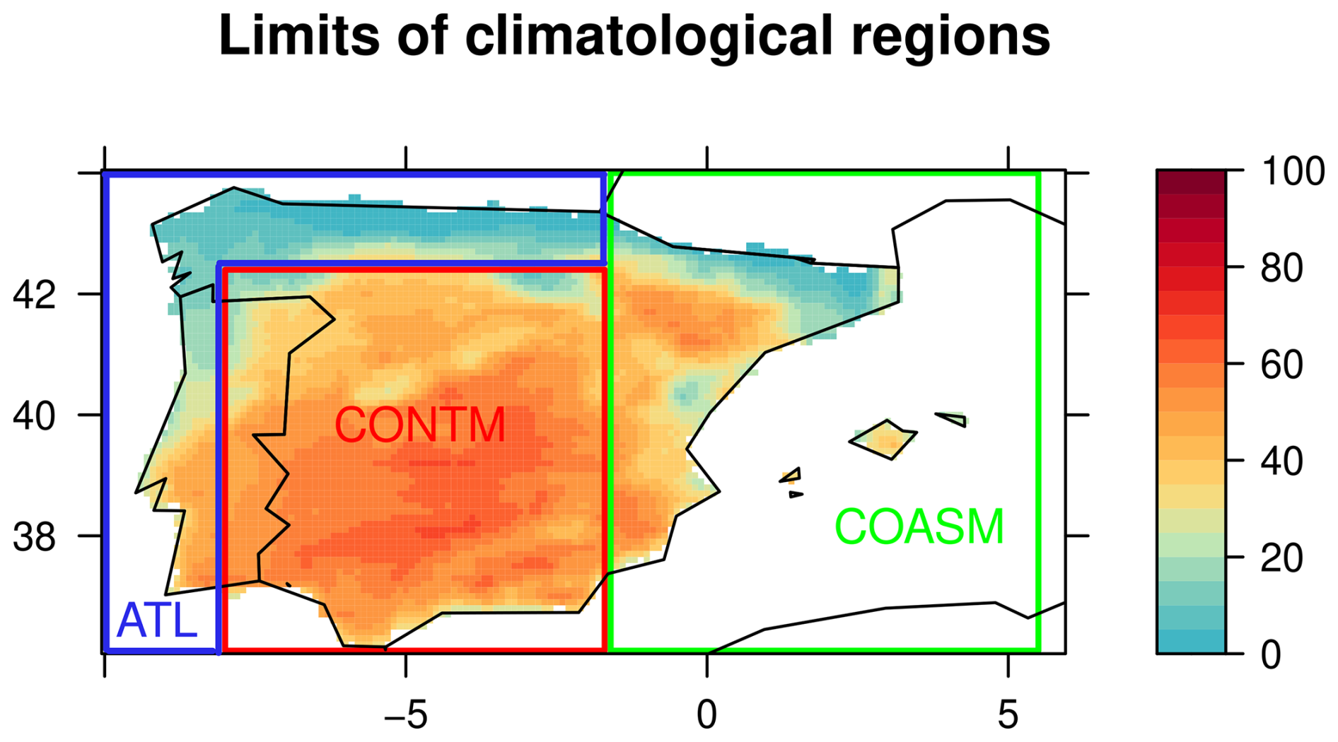
Figure A1 Climatological regions within the Iberian Peninsula used for XAI analysis in Fig. 6. Blue, green and red rectangles indicate ATL (Atlantic), COASM (Coastal Mediterranean), and CONTM (Continental Mediterranean) regions respectively.

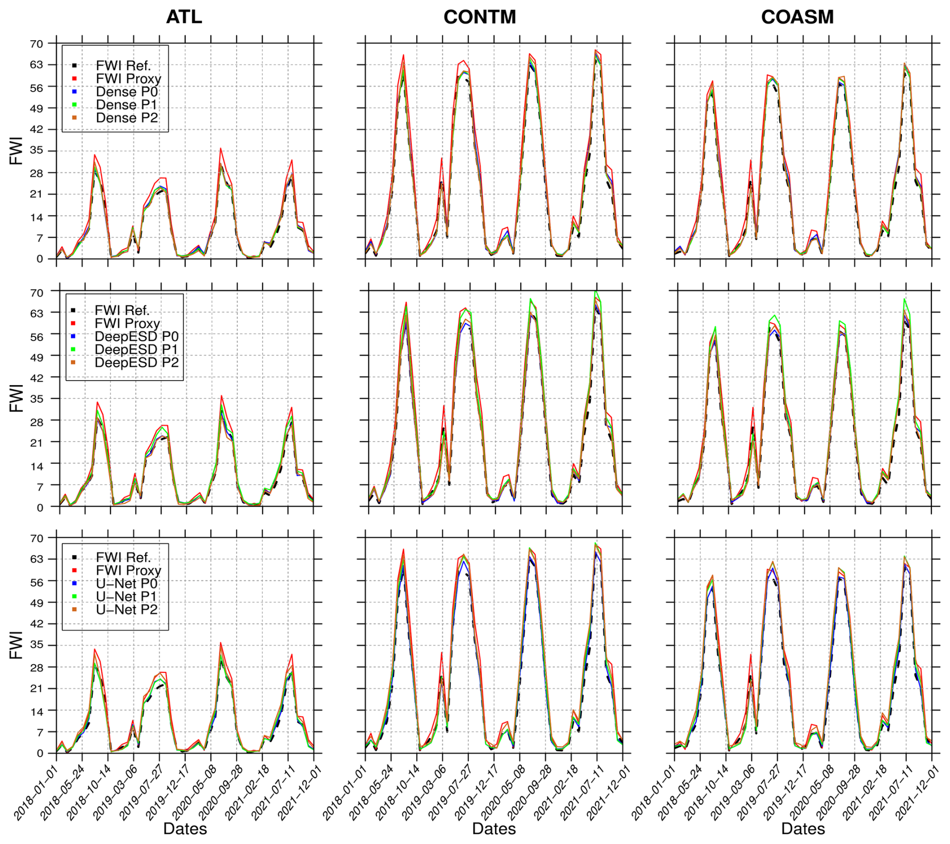
Figure A2 Monthly, spatially aggregated time series by climatological region for the reference FWI, the Proxy FWI, and the DL-based estimates over the 2018–2021 test period. The first, second and third row show the results for the Dense, DeepESD and U-Net models respectively.

Appendix B: ERA5-Land limitations

In this section, we highlight the existent limitations in using ERA5-Land data in our analysis due to the inherited biases in ERA5-Land compared with observation data. ERA5-Land, like other reanalysis products, is subject to inherent biases that arise from the limitations of the numerical models and data assimilation techniques used in its generation. These biases reflect systematic deviations from ground-based observations and can affect the reliability of the dataset for certain applications. Therefore, although ERA5-Land provides a valuable, spatially and temporally consistent climate dataset, its outputs should be used with caution and validated against local observations whenever possible.

In Fig. B1, we illustrate the ERA5-Land biases in some stations in Spain with respect to observation data provided by the Spanish Agency of Meteorology (AEMET).

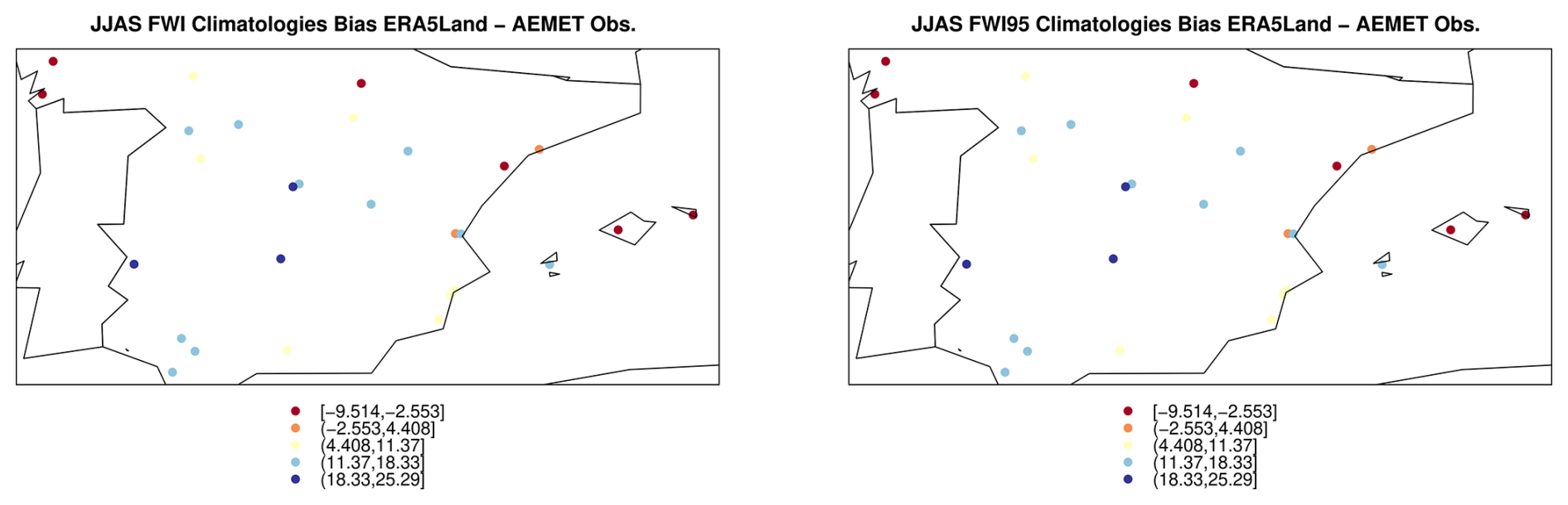
Figure B1 Biases between observational FWI data from the Spanish Agency of Meteorology (AEMET) and the FWI resulting from ERA5-Land computations. Top figure indicates de bias for the mean FWI, while bottom figure indicates it for the FWI95.

Appendix C: QQ-plot assessment

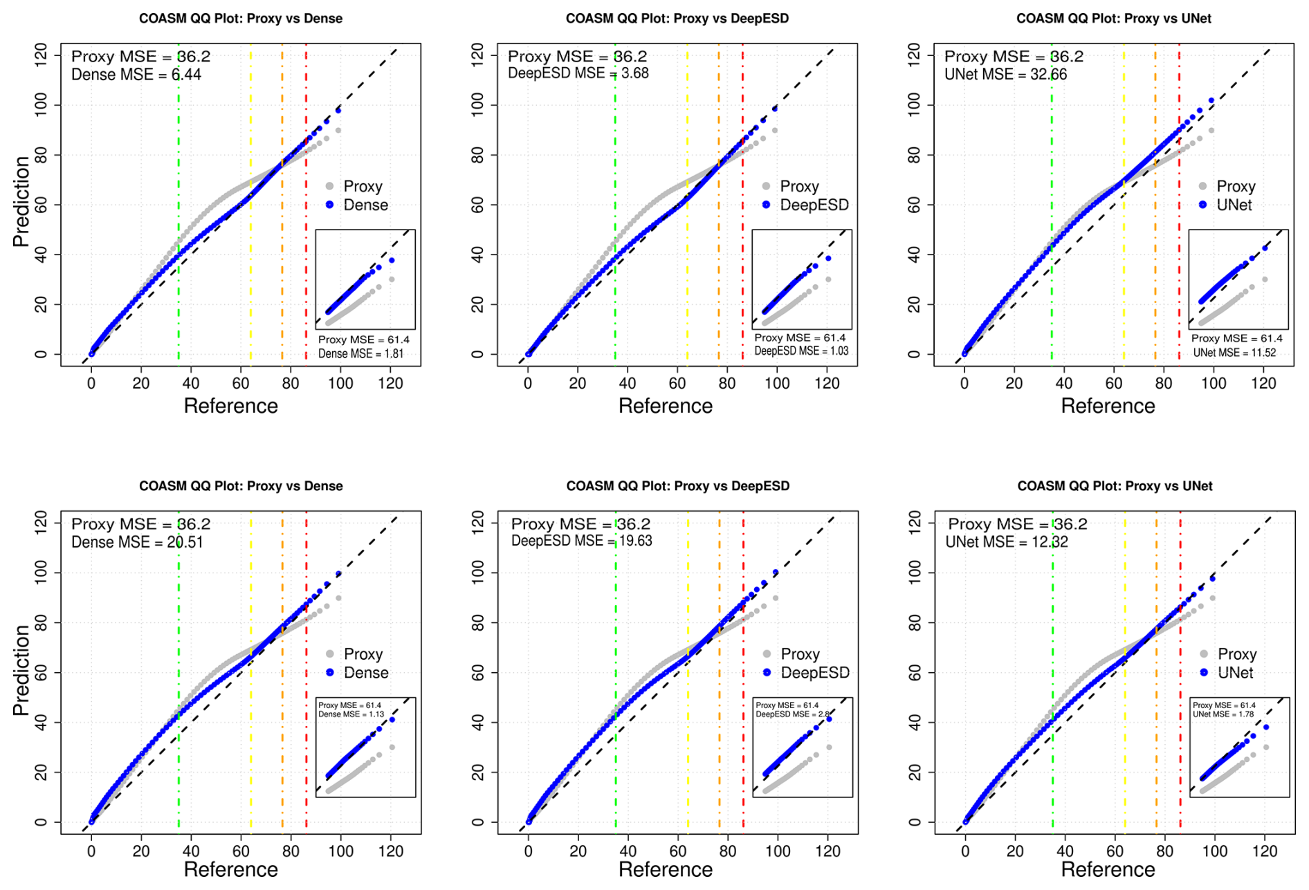
Figure C1 Quantile-Quantile (QQ) plots comparing the Proxy FWI (in grey) and DL model results (in blue). The results for the Coastal Mediterranean (COASM) (Fig. A1 for the subregion boundaries). Dash-dotted vertical lines indicate different fire danger levels established by the Agencia Estatal de Meteorología (AEMET). Fire danger levels are defined as follows: low (below the green line), moderate (between the green and yellow lines), high (between the yellow and orange lines), very high (between the orange and red lines), and extreme (above the red line). The Mean Squared Error (MSE) for both results is displayed in the top right corner. A box in the bottom right provides an amplified view of QQ plot focused on values above the 95th percentile (extreme danger), along with the corresponding MSE values under the box. First row indicates the results for models trained with MSE, and the second provides the models with ASYM as loss function.

Appendix D: Sensitivity analysis of deep learning models and evaluation of other predictors sets

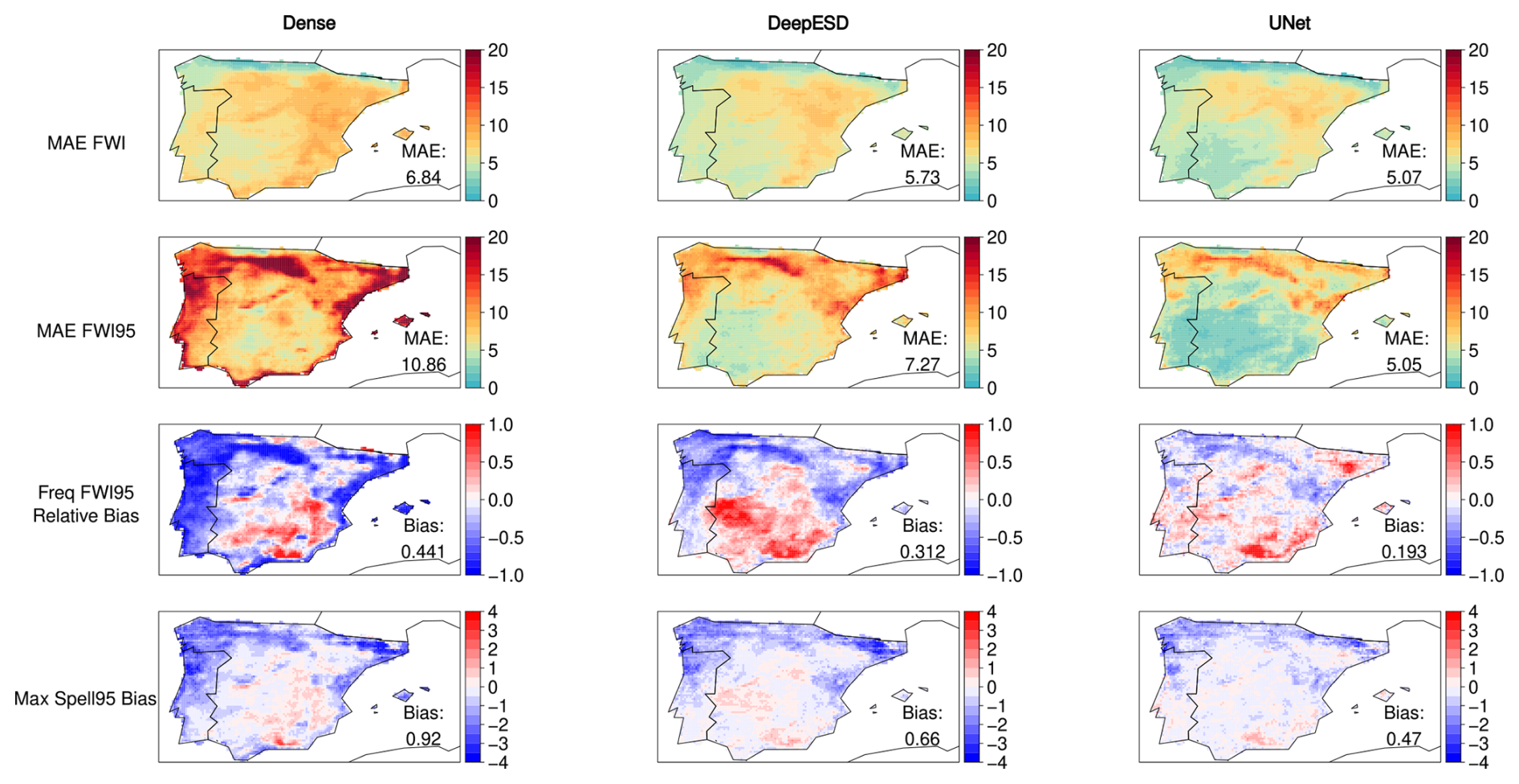
Figure D1 Results from the Dense, DeepESD and U-Net model trained with 12:00 UTC input variables (temperature, 24 h-accumulated precipitation, relative humidity and wind speed). The maps display differences relative to the reference FWI for the fire season (June–September) during the test period (2018–2021) for the validation indices. The MAE value inside the map represents the spatially aggregated mean absolute error of the deep learning predictions with respect to the FWI reference, while Bias denotes the spatially averaged bias in absolute value.

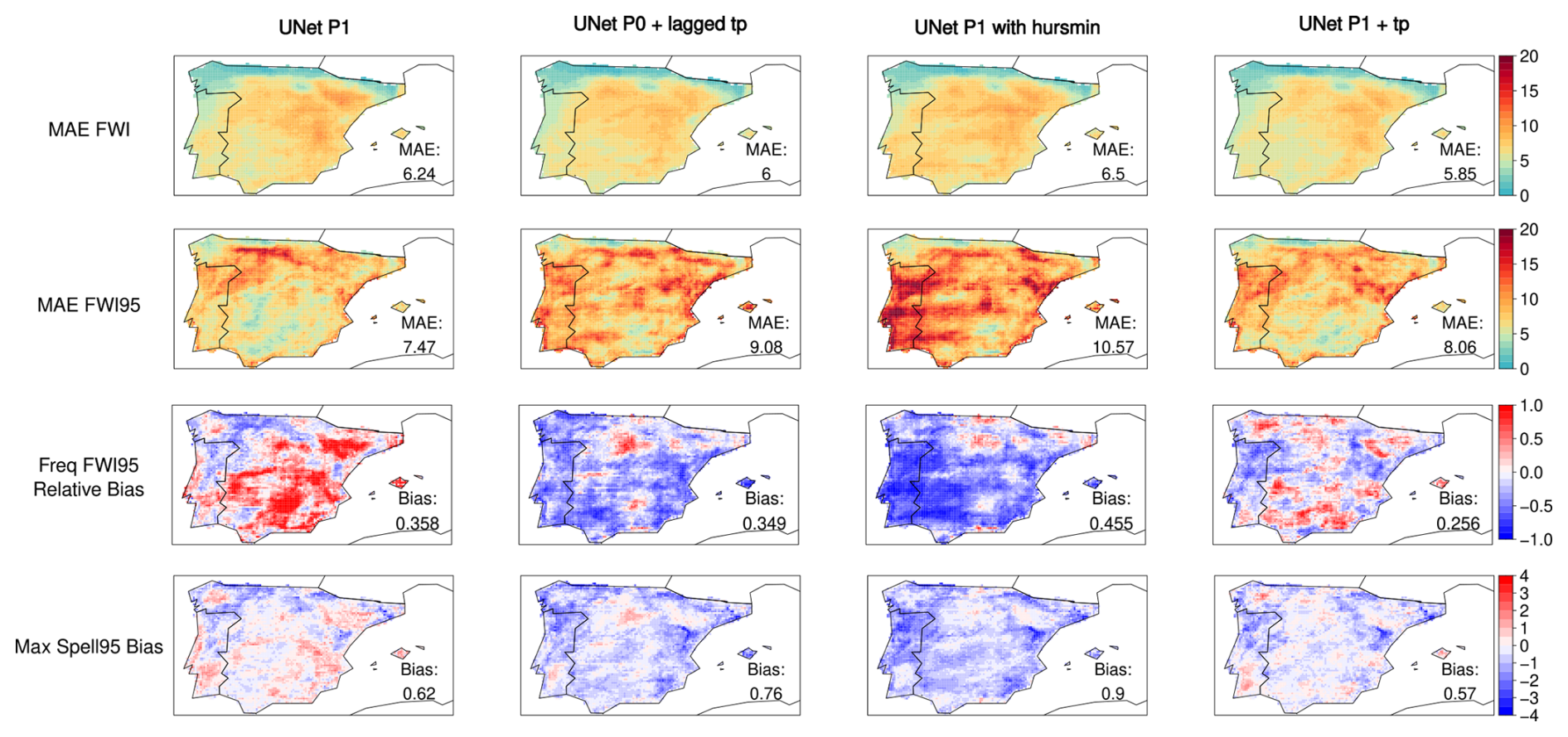
Figure D2 Results from the U-Net model trained with the P1 predictors set (see Table 1), trained with P0 and adding the 24 h lagged precipitation, trained with P1 adding minimum relative humidity instead of daily mean relative humidity and trained with P1 adding precipitation. The maps display differences relative to the reference FWI for the fire season (June–September) during the test period for different validation indices. MAE represents the spatially aggregated mean absolute error of the deep learning predictions with respect to the FWI reference, while Bias denotes the spatially averaged bias in absolute value.

Appendix E: Temporal dynamics and Persistence of Fuel Moisture Codes

Figure E1 highlights the ability of the DL-based emulators to reproduce the temporal evolution of the main fuel moisture codes under different predictor configurations for the CONTM region (see Fig. A1). In this Appendix, we evaluate the CONTM region because it is characterized by persistent and prolonged droughts across the Iberian Peninsula. Furthermore, the results obtained for the other regions exhibit similar behavior, making the CONTM region representative of the overall patterns. A clear scale-dependent behavior emerges, consistent with the intrinsic memory of each component. For the FFMC, which is characterized by short-term dynamics, the emulators show very high fidelity, accurately capturing both the amplitude and high-frequency variability of the reference signal. The DMC, with an intermediate memory, is also reasonably well reproduced, although with some local discrepancies in peak magnitude and timing. In contrast, the DC reveals a more pronounced limitation. While the emulators successfully reproduce the seasonal cycle and overall variability, they exhibit reduced temporal persistence compared to the reference, resulting in noisier time series and a weakened autocorrelation structure. This behavior reflects the difficulty of reproducing long-memory processes using architectures that rely primarily on instantaneous predictor–target mappings. These results suggest that, although the convolutional and dense architectures tested are highly effective for spatial reconstruction and short- to medium-term variability, they are less suited to capture the temporal coherence of slowly evolving indices such as the DC. Alternative architectures explicitly designed to model temporal dependencies, such as ConvLSTM networks (see  Mirones et al., 2025, for an application to FWI downscaling), could potentially alleviate this limitation, although their computational cost remains a constraint in large-domain applications such as the one considered here.

Importantly, this limitation does not appear to be driven by the exclusion of precipitation from the predictor set. Both configurations considered (P0, including precipitation, and P1, excluding it) show a comparable loss of temporal persistence in the DC. This suggests that the reduced autocorrelation structure is not primarily due to missing information, but rather reflects the intrinsic difficulty of capturing long-memory processes with architectures that do not explicitly model temporal dependencies.

To complement this qualitative assessment of the temporal behavior, we next provide a quantitative evaluation of temporal persistence. The integral timescale (τ) is used as a measure of temporal persistence, computed here as the e-folding time of the autocorrelation function of anomaly time series (daily values with the corresponding monthly mean removed), up to a maximum lag of 30 d (τ₃₀). It represents the characteristic time over which the signal remains temporally correlated, with larger values indicating stronger memory and smoother temporal evolution.

Table E1 provides a quantitative assessment of the temporal persistence of the emulated series through the integral timescale τ₃₀. A clear scale-dependent behavior emerges across the different fuel moisture components. For the FFMC, characterized by short memory, the emulators reproduce the temporal structure with high fidelity, showing negligible bias in τ₃₀. In contrast, the DMC exhibits a systematic underestimation of persistence, and this effect becomes particularly pronounced for the DC, where τ₃₀ is strongly underestimated in both predictor configurations. For the DC, the reference value (τ≈16 d) is reduced by more than 50 % in P0 and by nearly 80 % in P1, indicating a substantial loss of long-term memory and an over-responsive temporal behavior. Importantly, this limitation is observed even when precipitation is included in the predictor set (P0), suggesting that it cannot be primarily attributed to missing inputs, but rather to the limited ability of the employed architectures to capture long-memory processes. These results are consistent with the qualitative analysis of the time series (Fig. E1) and confirm that the performance of the DL emulators decreases with the temporal persistence of the target variable. Moreover, the RMSE values shown in Fig. E1 provide a complementary view of model performance. For the DC, errors are substantially larger than for the other components and increase when precipitation is excluded (P1), although they remain high even when precipitation is included (P0). In contrast, DMC and FFMC show much lower RMSE values, with negligible sensitivity to the inclusion of precipitation. This behavior is fully consistent with the persistence analysis based on τ₃₀ and supports the interpretation that the main limitation for DC arises from the representation of long-memory dynamics rather than from missing predictor information.

Table E1 Integral timescale (τ₃₀) and bias by FWI component, considering the test period predictions of the region CONTM.

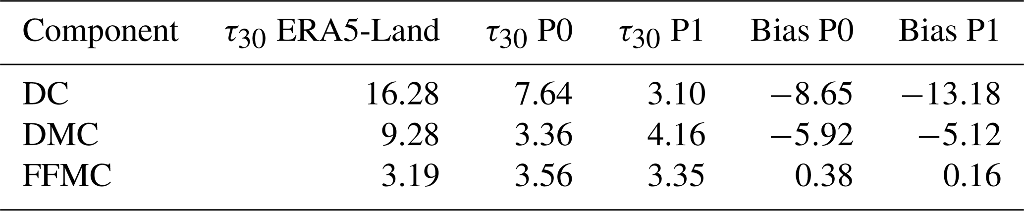
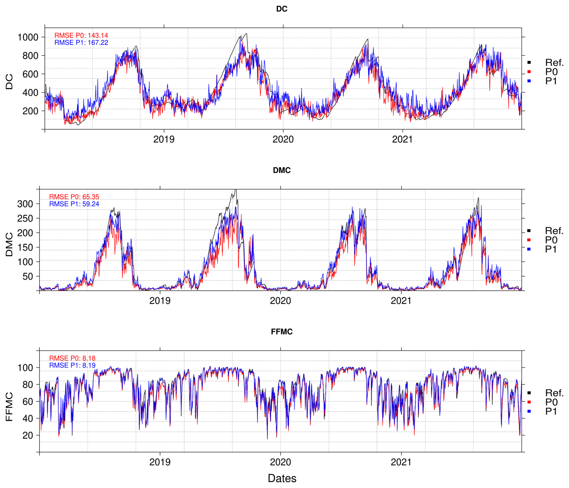
Figure E1 Daily, spatially aggregated time series for the reference, and the DL-based estimates considering the input sets P0 and P1 (see Table 1) over the CONTM region (see Fig. A1) during the 2018–2021 test period. The first, second and third row represents the Drought Code, the Duff Moisture Code and the Fine Fuel Moisture Code respectively.