Beyond the 100-year flood: probabilistic flood hazard assessment for King and Pierce Counties under future climate scenarios

Coastal regions across the globe, including the Salish Sea, are becoming increasingly vulnerable to compound flooding due to the interaction between storm surge, tides, and river outflow. This hazard is anticipated to increase under sea level rise and climate change. This research offers a high-resolution flood hazard mapping approach for King and Pierce Counties of Washington State (United States of America) using the SFINCS (Super-Fast INundation of CoastS) model to facilitate a Continuous Flood Response Modeling (CFRM) framework wherein decades of dynamic coastal and fluvial processes are simulated. By applying a cell-by-cell extreme value analysis, we predict flood areas for return periods of 1 to 100 years and compute the Expected Annual Flooded Area (EAFA) as a probability-weighted indicator of flood exposure. Validation of the model against NOAA and USGS gauge data demonstrated good skill (RMSE: 14–17 cm for coastal water levels; unbiased RMSE: 49–116 cm for river water levels), while comparison with FEMA Special Flood Hazard Areas showed high spatial agreement of flooding (hit rates: 0.75–0.83). The statistical analysis of the historical flooding timing showed that the 28 December 2022, event was primarily responsible for the majority of historical flooding in the region. Climate simulations for today indicate an EAFA range of 56–200 ha in King County and 250–644 ha in Pierce County. Projections of future changes show that the primary driver of increasing flood extent is sea level rise (an increase of 80 %–360 % with 1m SLR), while climate change drivers, such as changes to storm patterns, reduce hazards minimally. A threshold was also identified where there is a substantial increase in the area of land that is flooded when sea levels rise above 100–150 cm. Finally, it was found that simple deterministic flood maps may underrepresent flood hazard by approximately 0.5 m if not all contributing factors are considered. Therefore, these findings provide evidence supporting the use of integrated measures of flood hazard, such as EAFA, to inform more rational and spatially responsive flood risk management.

1 Introduction

Coastal and estuarine communities are increasingly vulnerable to flooding due to the combined effects of sea level rise (SLR), storm surges, high tides, and fluvial discharge. Approximately 600 million people globally live less than 10 m above mean sea level, a number projected to exceed 1 billion by 2050, and accelerating SLR could displace many and incur trillions of dollars in annual flood damages by the end of the century (Barnard et al., 2019). Two of the most populated counties in Pacific Northwest (PNW) in the state of Washington are King County and Pierce County, which contain the major metropolitan areas of Seattle and Tacoma, respectively, and lie adjacent to the Salish Sea, a large transboundary estuary characterized by complex bathymetric features, strong tidal forcing, and variable atmospheric conditions (Grossman et al., 2023). The combined impact of projected sea-level rise along the shorelines and increased river flow can produce compound flooding events that are significantly more destructive than either type of flooding event individually (Ali et al., 2025; Wahl et al., 2015). Further adding to the need to address this problem is the anticipated continued expansion of urban populations and the removal of natural buffers against flooding in low-lying coastal regions (Wing et al., 2022).

Historical analyses of flooding are generally single-event (or deterministic) in their approach and thus fail to model the interrelatedness of and temporal variability in the component drivers of a compound flood event (Green et al., 2025). As such, the research community has increasingly turned toward the application of probabilistic methodologies to assess flood risks through the utilization of copulas to maintain the relationship(s) among flood drivers (Couasnon et al., 2020), the joint probability method for tropical cyclones (Resio and Irish, 2015) and response-based methodologies which utilize the output of simulations to estimate flood probabilities (Gori et al., 2020). Cell-by-cell extreme value analysis has been used in numerous contexts, including global storm surge reanalysis (Muis et al., 2016), mid-Atlantic estuary flooding (Deb et al., 2025), and coastal risk assessment under climate projections (Son et al., 2025).

In particular, continuous simulation (CS) methodologies have been developed as an alternative to event-based flood assessment methods. The CS methodologies provide greater linkage to the physics of the processes involved and eliminate the assumption associated with design conditions (Viviroli et al., 2022). This study combines response-based compound flood modeling with continuous simulation (i.e., decades-long boundary forcing including tides, surge, and river discharge) and is termed here Continuous Flood Response Modeling (CFRM). The main distinction is that flood probabilities are derived empirically from the resulting simulated responses at each location, rather than from driver statistics or pre-selected events. CFRM also enables attribution of controlling drivers (coastal, fluvial, or compound), timing, and relative contributions to extreme water levels and associated flooding risk.

We implement the CFRM framework for assessing compound flood hazard in King and Pierce Counties, Washington, using the Super-Fast INundation of CoastS (SFINCS) model (Leijnse et al., 2021). Our implementation builds on the Coastal Storm Modeling System (CoSMoS; Barnard et al., 2019; O'Neill et al., 2018) and expands the Puget Sound implementation of Nederhoff et al. (2024) by improving the representation of coastal-riverine interactions. This framework provides three advances: (1) over 100 years of continuous boundary forcing to allow for the empirical estimation of return levels without fitting analytical extreme-value distributions; (2) modifications were made to SFINCS to record the timestamp of the maximum water level at each grid cell to enable the spatially explicit attribution of flood hazard; and (3) comparisons were made between the deterministic single-event methodologies and the CFRM methodology to illustrate that differences in compound flood zone can be up to 0.5 m and exhibit systematic spatial patterns that reflect the transition from coastally to fluvially dominated forcing. The modeling system was validated by comparing modeled water levels and flood extent to observed values. In addition, the modeling system was applied to evaluate the current and future flood hazards due to sea level rise (SLR) and climate change. We also compute the Expected Annual Flooded Area (EAFA), a probability-weighted metric that incorporates flood hazard across all return periods to support risk-informed planning.

Figure 1 King and Pierce Counties are located in the Pacific Northwest of the United States of America (A). Panel (B) provides an overview of the area of interest in King County (blue domain) and Pierce County (green domain), Washington, and the SFINCS model domains. Panel (C) provides a detailed view of Pierce County and Panel (D) provides a detailed overview of King County. Note that there are five inflow boundary conditions in total, but due to partial overlap between panels (C) and (D), some boundaries appear duplicated. Two NOAA stations are included 944713 (Seattle) and 9446484 (Tacoma) and 5 USGS stations (12096500, 12101500, 12113000, 12113344, 12113390) – see NOAA (2025) and U.S. Geological Survey (2025) for more information. Background: Esri World Imagery basemap. Sources: Esri, Maxar, GeoEye, i-cubed, USDA FSA, USGS, AEX, Getmapping, Aerogrid, IGN, IGP, swisstopo, and the GIS User Community | Powered by Esri.

2 Study site: King and Pierce County

The Salish Sea is one of the most significant and complex transboundary estuaries in North America. It spans across British Columbia, Canada, and Washington State, USA. It was formed from flooded glacial valleys, and it is composed of several different basins, including the Strait of Georgia, Puget Sound, and the Strait of Juan De Fuca. King County and Pierce County are located in the Puget Sound. The two counties have a total area of over 10 000 km² and contain the cities of Seattle (located in King County) and Tacoma (located in Pierce County), representing dense populations, high levels of urban development, and a great deal of economic and environmental value in the coastal zone (Fig. 1). Land use in King and Pierce County is diverse, from the highly developed urban areas of Seattle and Tacoma to the productive agricultural lands found in the lower elevation areas of the delta and tidal flats that are at risk for flooding (Grossman et al., 2023).

Topography in this area includes elevations ranging from approximately sea level to greater than 4300 m at Mount Rainier. The Cascade glaciers feed numerous streams that produce river systems of steep gradient and high velocity, carrying water and sediment from alpine to marine environments (Sisson et al., 2001). The largest rivers in King County are the Duwamish and Green Rivers, while the largest river in Pierce County is the Puyallup River. All of these rivers drain large watersheds that include agricultural and urban areas before emptying into Puget Sound. At the mouth of each of these rivers is a broad estuary and delta that is susceptible to compound flooding resulting from both coastal and fluvial source floodwaters.

Tides in the Salish Sea follow a mixed semi-diurnal meso-tidal cycle with tidal amplitudes increasing from approximately 2.4 m at the ocean mouth at Neah Bay to 4.4 m further inland (e.g., Olympia) and very fast currents (>1 m s⁻¹) that occur through restricted passages such as Admiralty Inlet (Grossman et al., 2023). Storm surges are a result of low-pressure weather systems that develop over the eastern Pacific Ocean and move onshore between Oregon and Vancouver Island (Yang et al., 2019). Coastal water levels reach their highest during storms when the combination of remote sea level anomaly (SLA) due to changes in atmospheric pressure away from the coast, the inverse barometer effect, and the effects of local winds creates high water levels. Typically, the amplitude of the maximum surge is less than or equal to ∼1 m (Grossman et al., 2023). Wave climates within the Salish Sea vary geographically. Swell waves with long periods (usually greater than or equal to 10 s) dominate the outer coast and the western Strait of Juan de Fuca. However, wind-sea waves with short periods (less than 5 s) and low wave heights (less than 2 m) are the primary waves affecting Puget Sound (Crosby et al., 2023).

Both historical and recent events show that the area is susceptible to compound flooding. A recent “King Tide” event in Seattle's South Park neighborhood on 28 December 2022, reached a 3.8 m+ NAVD88 at NOAA Seattle Gauge #9447130. This event caused extensive flooding due to a combination of snowmelt, a low-pressure system, and runoff from stormwater (Thomas, 2023). Historical flooding occurred along the Nisqually and Green Rivers in December of 1975 (U.S. Army Corps of Engineers, 1977). Flooding also occurred in November of 1990 along the rivers of Pierce County (Hubbard, 1994). Each of these flooding events highlights the need to model compound flood risk and to consider the spatial and temporal variability of the risk in modeling the compound flood risk, especially given projections of more intense rainfall and reduced snowpack and glaciers in the near future, anticipated to drive complex changes in water and sediment runoff (Lee et al., 2016).

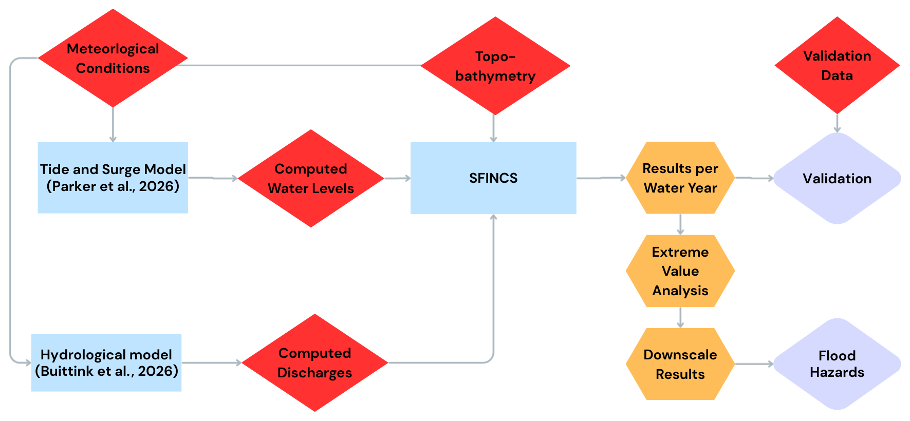
Figure 2 Conceptual workflow of the CoSMoS flood modeling framework. Blue rectangles represent model components, red diamonds indicate input data sources, orange hexagons denote analysis steps, and purple rounded diamonds show the main outputs of the study.

3 Materials and methods

3.1 Overview

The modeling strategy adopted in this study draws upon CoSMoS (Barnard et al., 2014), originally developed for California and later adapted for Washington State (Crosby et al., 2023; Grossman et al., 2023; Nederhoff et al., 2024). Figure 2 displays the conceptual framework as applied here. Overland flooding was simulated using the open-source model SFINCS (Leijnse et al., 2021), which was selected for its computational efficiency and ability to represent dynamic flood processes. Two high-resolution model domains were constructed for King and Pierce Counties, incorporating high-resolution topobathymetric data and land cover (Sect. 3.2.1). Boundary conditions for water levels and river discharges were provided from multi-century climatological datasets (Sect. 3.2.2). The modeling was conducted in two phases: first, the reanalysis period was simulated and validated against observational datasets (Sect. 4.1). Second, future climate conditions were simulated under multiple SLR scenarios. Compound flood outputs from these simulations and extreme value analysis were used to estimate flood frequency and were subsequently downscaled to higher spatial resolution (Sect. 4.2). The following sections describe the input data, model components, numerical methods, and computational framework in greater detail.

3.2 Input data

3.2.1 Static data: topobathymetry and land roughness

Elevation data for the entirety of the coastal regions of King and Pierce Counties were derived from the Coastal National Elevation Database (CoNED) topographic model of Puget Sound (Tyler et al., 2020). The CoNED dataset provides a seamless digital elevation model (DEM) at 1 m resolution, constructed from the latest high-resolution datasets, including light detection and ranging (LiDAR) topography, multibeam and single-beam bathymetry, and other topographic and bathymetric sources. These datasets were merged into a continuous surface to ensure spatial consistency and accuracy. For this study, CoNED data were extracted to create DEMs necessary for running the SFINCS model. The CoNED DEM has a root-mean-square error (RMSE) of 22 cm, which reflects its reliability for this type of coastal hazard analysis.

The subsampled CoNED DEMs were used to characterize the nearshore zone, beach areas, riverine channels, and levees as accurately as possible. Elevation data are the first-order control on flood hazard modelling fidelity, and a high resolution and level of detail are critical for capturing the hydrodynamic processes that govern coastal and riverine flooding. Early model runs, however, revealed inaccuracies in the representation of riverine bathymetry. To address this, additional data were utilized to infer channel bathymetry characteristics for the major river systems. Modified riverine bathymetry was found to improve the representation of channel morphology and flow dynamics within the SFINCS simulations. In particular, a trapezoidal channel shape was imposed along the Green and Puyallup Rivers to replace the hydro-flattened bathymetry, which was too shallow. The channel centerlines were defined by digitizing a line along the thalweg, and cross-sections were deepened to a trapezoidal profile to improve hydraulic connectivity in the model.

The National Land Cover Database (NLCD; Homer et al., 2020) was utilized to define spatially variable roughness over the SFINCS model domain. Comparable translations, as in Nederhoff et al. (2021), were used to convert land cover classes into Manning n friction values. This approach enabled the representation of heterogeneous surface characteristics, with roughness values ranging from 0.020 for open water to 0.15 for forests. Open water friction was set to a constant 0.020 value and was thus not used for calibration. This spatially variable roughness enhances the model's ability to simulate flood behavior across a variety of land cover and hydrologic regimes.

3.2.2 Dynamic forcing conditions: water levels and discharges

Water levels and wave heights were extracted from regional Delft3D FM and SWAN modeling efforts (Parker et al., 2026). Specifically, a Delft3D Flexible Mesh (Delft3D FM) model was used to compute tides and surges across the Salish Sea. The model exhibited high skill in replicating still water levels compared to six National Oceanic and Atmospheric Administration (NOAA) tide stations and seven U.S. Geological Survey (USGS) tide gauges across the 2017–2019 validation period (Fig. 1), with a mean error of approximately 10 cm (Grossman et al., 2023). Still water levels (water levels driven by tides, steric sea level anomalies, and storm surges) were directly extracted from the regional Delft3D FM model at ∼20 m depth and at an approximate alongshore spacing of 500 to 1000 m (see white circles in Fig. 1). Still water levels were imposed as time-varying water level boundary conditions along the open coast of the SFINCS domains. Waves were computed as a sum of locally generated wind waves and the linear transformation of the Pacific Ocean swell. This approach enables quick wave predictions at high spatial resolution, where wave heights are added in quadrature and wave periods are determined by a weighted average, making long-term regional simulations possible, with skills similar to standard SWAN implementations (Crosby et al., 2023). Wave height was converted into wave setup through the 20 % of the wave height approximation commonly used in coastal engineering (e.g., Vousdoukas et al., 2018) and added to the still water levels computed by the Delft3D model. This simplified approach was chosen for efficiency, but could misrepresent run-up in some locations.

Stream inflow discharges were simulated using the wflow hydrological modeling framework (van Verseveld et al., 2024). The wflow model allows for the simulation of key catchment hydrological processes, including precipitation, interception, snow accumulation and melt, evapotranspiration, soil water, surface water, and groundwater recharge, within a fully distributed environment. Discharges were imposed at five locations (1 in King County and 4 in Pierce County), at approximately +20 m NAVD88, which is considered outside the zone of tidal influence (Fig. 1 – blue circles). Discharges were typically within a 20 % error margin of observed flows, based on the calibration/validation of the wflow model in the region (Buitink et al., 2026). For more information on this regional modeling work, one is referred to Buitink et al. (2026).

All model domains were forced using meteorological conditions, including wind speed and mean sea level pressure. These meteorological inputs were applied in the upstream/regional models (e.g., atmospheric forcing for Delft3D FM and wflow), ensuring that storm effects were represented in the boundary water levels and river inflows passed to SFINCS. No direct wind or rain forcing was applied within the SFINCS domains. For the hindcast (validation) period from 1941 to 2022, meteorological inputs were based on ERA5 reanalysis data (Hersbach et al., 2020). For the projection period, conditions were derived from the Coupled Model Intercomparison Project – Phase 6 (CMIP6). An ensemble of 7 CMIP6 models from the High-Resolution Model Intercomparison Project (HighResMIP, Haarsma et al., 2016) was used with the SSP5-8.5 greenhouse gas concentration scenario. Models from the HighResMIP project were selected for their higher spatial resolution (25–50 km), which is expected to improve the representation of coastal storm events that are inadequately resolved by the native resolution of most general circulation models (GCMs; Roberts et al., 2020). As a compromise for higher resolution, models in the HighResMIP project were run for a shorter simulation time (1950–2050) than other CMIP6 models. Therefore, conclusions regarding temporal changes in forcing are limited to this time horizon. More details on the specific CMIP6 model iterations used, and their implementation in the regional framework, can be found in Parker et al. (2026).

To assess the impact of SLR on flooding in King and Pierce Counties, seven SLR scenarios were selected: 0, 0.25, 0.50, 1.00, 1.50, 2.00, and 3.00 m above mean sea level in the year 2005. These scenarios were selected to bracket the potential magnitudes of SLR without consideration of particular time frames so that flexibility is provided for future re-analysis as relative SLR projections are refined. This response aligns with the suite of SLR projections for the U.S. West Coast through the year 2100 presented by Sweet et al. (2022) and previous CoSMoS modeling research (Barnard et al., 2014).

3.3 Validation data

3.3.1 Coastal water levels: NOAA

Time series of observed water levels at NOAA stations (Fig. 1 – red circles with prefix “NOAA” labeling) across the study area were utilized to validate the model. Hourly water levels relative to NAVD88 were obtained from two NOAA stations for the period 1942–2022. The Seattle, WA station (Station ID: 9447130) has a continuous record, while the Tacoma, WA station (Station ID: 9446484) started operating in 1996 (NOAA, 2025).

3.3.2 Riverine water levels USGS

Stream time series of observed water levels from USGS (Fig. 1 – red circles with “USGS” prefix labeling) were used to validate the inland conditions model. River stage data from 2007 to 2022 were collected at five USGS stations. Because the reference level of stage measurements can be non-uniform, all the comparisons were adjusted to make a fair comparison between the model (referenced to NAVD88) and the USGS observed gage heights.

3.3.3 Flood extent: FEMA maps

Federal Emergency Management Agency (FEMA) Special Flood Hazard Areas (SFHAs) were used as reference data for a qualitative benchmark. While SFHAs are modelling products themselves and by no means represent truth, they are important regulatory products and widely used by communities. SFHAs illustrate zones of a 1 % annual chance of flooding (commonly referred to as the “100-year floodplain”) and are the primary regulatory flood zones mapped in FEMA's Flood Insurance Program. These zones are established through site-specific analysis that commonly involves hydrologic and hydraulic modeling, which may vary from simplifying assumptions to complex 1D or 2D simulations depending on local conditions and data availability. In this study, FEMA-provided vector shapefiles of the 1 % Annual Exceedance Probability (AEP) floodplain were used for comparison with simulated flood extents (Federal Emergency Management Agency, 2025). However, there are no detailed metadata available to describe the underlying data, making it nearly impossible to determine the data's age, resolution, or methodology for each jurisdiction. To allow for pixel-based validation, all FEMA shapefiles were rasterized to a 2 m resolution grid and reclassified into three classes: flooded (wet), not flooded (dry), and no data. These raster FEMA maps enabled pixel-by-pixel comparison to our modeled flood extents, from which we computed categorical skill metrics (hit rates, false alarm ratios, etc.) described in Sect. 3.3.

3.4 Numerical method: overland flooding with SFINCS

SFINCS (Leijnse et al., 2021; van Ormondt et al., 2025a) was used to simulate compound flooding processes, encompassing dynamic hydraulic phenomena such as tidal propagation and river runoff while ensuring computational efficiency (e.g., Sebastian et al., 2021). This combination of capabilities made SFINCS an ideal choice for predicting overland flooding in this study. Two computational domains were developed for King and Pierce Counties (refer to Fig. 1 – panels C and D), each constructed at a 50 m resolution, covering an average area of 3000 km². These domains incorporated 1 m resolution CoNED topobathymetric via subgrid tables (which store the elevation at 20 vertical levels) to preserve fine-scale topography within each 50 m cell. All simulations were conducted with advection enabled, turning SFINCS into a solver for the Simplified Shallow Water Equations (SSWE).

No calibration of the SFINCS computations was performed, as simulated regional water levels and riverine inflow discharges were directly imposed, and friction in open water was held constant. Overland flooding was allowed to infiltrate at a constant 2 mm h⁻¹ (representing low-permeability soils, Rawls et al., 1982), to provide a rudimentary representation of drainage and prevent indefinite ponding in flat areas. Rainfall or wind forcing were not directly applied in the model, but these factors were used to derive regional boundary conditions for water levels and discharges.

Simulations were conducted for complete water years (WY; a 12-month period from 1 October through the following 30 September and named for the year in which it ends), preceded by a 7 d initialization period (spin-up period). Key outputs recorded during the simulations included the maximum annual water level, the maximum depth-velocity product (m² s⁻¹), the duration that each cell remained wet using a minimum depth of 10 cm, and the time of maximum water level.

The model results were generated using a slightly modified version of the SFINCS “Dollerup” release from November 2023, which is available as open-source code on GitHub and through Deltares (van Ormondt et al., 2025b; https://github.com/Deltares/SFINCS; last access: 12 May 2026). In particular, we added new output functionality that tracks the moment of high water. These changes have recently been merged into the main trunk of the code on GitHub.

To account for uncertainty in boundary conditions, an additional two simulations were performed with altered “low” and “high” estimates of parameters. The low estimate reduced dynamic coastal water levels by 50 cm, lowered river discharge by 20 %, and increased weir crest elevations by 50 cm to represent a more conservative (lower hazard) scenario. Conversely, for the high estimate, the same parameters were adjusted with the same magnitude but in the opposite direction to simulate a more demanding (higher hazard) boundary condition. These are constructed to simulate a deterministic uncertainty bound, inspired by the 95 % confidence interval, based on normally distributed model residuals and ±2 times the root-mean-square error (RMSE) enclosing the likely range of flood response. A statistically rigorous 95 % confidence interval is not possible in this category of deterministic modelling (for example, DEM uncertainty must be properly propagated). The developed uncertainty bounds allow us to examine the sensitivity of predictions of flood extent to uncertainty in the dominant (hydrodynamic) inputs. Results from these High/Low hazard simulations are used later to define uncertainty ranges.

3.5 Computational framework, simulation period, and computational expense

The modeling framework was structured into three distinct phases: (1) reanalysis (hindcast) validation, (2) current climate projections, and (3) future climate projections.

During the validation phase, the model was validated over an 82-year reanalysis period spanning water years 1941 through 2022. Coastal water levels were validated using observations from two NOAA tide gauge stations (Seattle and Tacoma, WA), while inland water levels were assessed using data from five USGS streamgages distributed across King and Pierce Counties (Fig. 1).

To support extreme value analysis, the model was driven with 82 years of reanalysis boundary conditions (1941–2022) modelled with respective coastal water levels of Parker et al. (2026) and upstream modeled discharges by Buitink et al. (2026). Our approach included the generation of an additional 18 synthetic years with randomized tidal phasing, bringing the total timeseries to 100 years, ensuring adequate sampling of extreme events. Importantly, this method enabled an empirical estimation of 100-year return levels, avoiding the need to fit a theoretical extreme value distribution. In particular, the method from Nederhoff et al. (2024) for a synthetic record was utilized by randomly selecting a yearly non-tidal-residual (NTR) signal from the 82-year record. NTR refers to all non-tidal fluctuations in sea level and includes, for example, contributions from steric sea level anomalies and wind-driven storm surge. A uniform distribution shift from −1 to +1 d was applied to the time axis of the NTR to increase variability. Tides were generated from astronomical components computed from the tide-only regional model results. Discharge and wave conditions were assumed to be completely correlated with NTR, and associated wind and wave conditions are directly used in model forcing.

In the future climate phase, the model was forced using the pseudo-global-warming (PGW) approach (Brogli et al., 2023). The PGW strategy consists of simulating the current conditions with boundary conditions modified by the climate change signal (delta). In this case, the same reanalysis 100-year simulation was re-run with all boundary conditions (water levels and riverine discharges) modified by a calculated climate change signal. The utilized delta was calculated by running the regional models (both water level and streamflow), forced by an ensemble of CMIP6 models. The CMIP6 forced ensemble was run for both a historical and future period, with the change (the delta in the PGW method) then calculated at all boundary forcing points used in this study. The delta was calculated by computing the difference between the future and historical cumulative distribution function (CDF) at all quantiles in the CDF, allowing a variable delta across the CDF. This approach allows flexibility in how water levels might change, for example, extremes increasing while the average water level stays the same. In essence, this applies a quantile-dependent shift to every time step of the historical boundary conditions so that their statistical distribution matches that projected for mid-century climate. To allow for seasonal differences in the climate change signal, this delta was calculated for each month of the year. The full ensemble of calculated deltas (7 climate models, 12 months, all quantiles) was reduced by taking the average across the CMIP6 ensemble members, with averaging used to reduce individual CMIP6 bias and improve robustness of the resulting calculated delta signal. This delta was then applied to the full timeseries of the current climate projections period to produce a new boundary forcing PGW timeseries representing the future period. Simulations using this PGW future climate were then conducted for multiple SLR scenarios to evaluate the sensitivity of flood hazards to different future climate trajectories. In this way, future changes to flood hazards are segmented into 2 signals: a climate change forcing signal (provided using the PGW method) and an SLR signal (implemented as a change to mean sea level). The PGW approach was chosen to minimize the effects of bias in the individual GCMs. The reanalysis timeseries represents the best possible basis for hazard characterization, with data assimilation enforcing dynamic consistency in the study region as well as at larger scales. The PGW method seeks to leverage this robust timeseries basis, but with changes into the future included (via the delta method, which limits bias from individual CMIP6 models). The drawback of this method is that only changes in the magnitude of forcing are modelled, not in frequency or timing.

Flood hazards are often defined by wet areas based on a specific flood depth threshold, typically 10 or 15 cm (e.g., Wing et al., 2017). In this paper, we apply three classes of flood severity: nuisance flooding (depth >10 cm), hazardous flooding (depth >30 cm), and severe flooding (depth >100 cm). The flood hazards were analysed over a full range of return periods from 1 to 100 years. We also computed the Expected Annual Flooded Area (EAFA), as a probability-weighted sum of flood extents for all return periods, and computed this for each severity class separately (Vousdoukas et al., 2023). To focus on event-driven flooding, grid cells that flood during regular daily tidal conditions were not included in these calculations.

All the simulations were executed on the USGS Hovenweep platform (Falgout et al., 2025). A single simulation run (one water year) required approximately 36 h to finish. We simulated the current climate scenario at mean sea level (0 m SLR) and at one elevated SLR level (1.0 m) to isolate SLR-only effects. Under future climate (PGW conditions), we ran the full set of seven SLR scenarios (0 through 3 m). In total, 5400 yearly simulations (7× SLR scenarios with future climate and 2× SLR for current climate, 3 uncertainty layers, and 2 domains) were conducted, totaling a computational effort of approximately 194 400 h. However, the actual computational burden was an order of magnitude higher due to additional sensitivity tests, calibration runs, and model refinements in an iterative stakeholder process. In order to quantify uncertainty in SLR projections, each scenario was rerun with both high and low estimates, totalling 2700 simulations. This extensive simulation effort offers robust statistical analysis, multiple scenarios to address the requirements of stakeholders, and testing to address both past and future flood conditions.

3.6 Model skill

To quantify the skill of the model to reproduce water levels of the current climate, several accuracy metrics were calculated: model bias, mean-absolute-error (MAE; Eq. 1), root-mean-square-error (RMSE; Eq. 2), and unbiased RMSE (uRMSE; RMSE with bias removed from the predicted value)

$$\begin{array}{}\text{(1)}& {\displaystyle }\mathrm{MAE}={\displaystyle \frac{\mathrm{1}}{N}}\sum \left(\left|y_i-x_i\right|\right)\text{(2)}& {\displaystyle }\mathrm{RMSE}=\sqrt{{\displaystyle \frac{\mathrm{1}}{N}}\sum (y_i-x_i{)}^{\mathrm{2}}}\end{array}$$

where N is the number of data points, y_i is the ith predicted (modeled) value, and x_i is the ith measurement. For stations without a reference level, we computed the unbiased RMSE and MAE, also referred to as uRSME and uMAE. Lastly, we compute the scatter index (SCI), which is a metric to express RMSE in a relative sense as a fraction of the RMS magnitude of the signal.

In addition to these continuous metrics, a binary skill classification was used to evaluate the model's ability to correctly predict wet and dry conditions (Wing et al., 2017). For this classification, model predictions were compared to observations using a contingency table with the following categories:

• True Positives (TP): Correctly predicted wet cells (M1B1)

• True Negatives (TN): Correctly predicted dry cells (M0B0)

• False Positives (FP): Predicted wet but dry benchmark cells (M1B0)

• False Negatives (FN): Predicted dry but wet benchmark cells (M0B1)

From this classification, the following skill metrics were derived:

$$\begin{array}{}\text{(3)}& {\displaystyle }\text{Hit\hspace{0.17em} rate\hspace{0.17em} index}\left(\mathrm{H}\right)={\displaystyle \frac{\mathrm{TP}}{\mathrm{TP}+\mathrm{FN}}}\text{(4)}& {\displaystyle }\text{False\hspace{0.17em} ratio\hspace{0.17em} index}\left(\mathrm{F}\right)={\displaystyle \frac{\mathrm{FP}}{\mathrm{TP}+\mathrm{FP}}}\text{(5)}& {\displaystyle }\text{Critical\hspace{0.17em} success\hspace{0.17em} index}\left(\mathrm{C}\right)={\displaystyle \frac{\mathrm{TP}}{\mathrm{TP}+\mathrm{FP}+\mathrm{FN}}}\text{(6)}& {\displaystyle }\text{Error\hspace{0.17em} bias\hspace{0.17em} index}\left(\mathrm{E}\right)={\displaystyle \frac{\mathrm{FP}}{\mathrm{FN}}}\end{array}$$

These binary skill metrics complement the continuous accuracy measures and provide a comprehensive evaluation of the model's performance, particularly for assessing its capability to predict flooding extents.

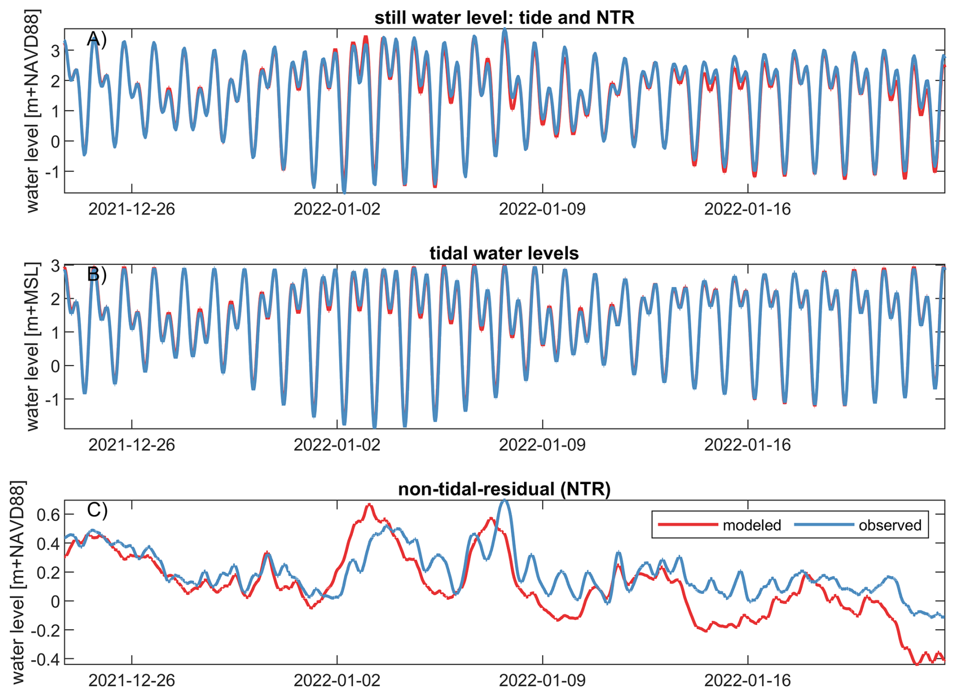
Figure 3 Comparison of coastal water levels at Seattle, WA (NOAA station #9447130): Comparison of modeled and observed still water levels for 1 month, including the decomposition into tidal (tide) and non-tidal residual (NTR) components. Panel (A) shows the observed and modeled still water levels, panel (B) highlights the modeled and observed tidal contribution, and panel (C) presents the NTR. Determination of the tidal signal was done in the same manner for both the modeled and observed signals.

4 Results

4.1 Validation

4.1.1 Coastal water levels

Modeled still water levels from WY1942 until WY2022 were validated against gauge data. An example time series of 1 month of water level at the tide gauge station Seattle, WA (NOAA station #9447130), including the decomposition in tide and NTR, is shown in Fig. 3. Table 1 contains a summary of skill scores for still water level and tide of 2 NOAA gauges for 82 years of modeled water years in terms of RMSE, SCI, MAE, and bias. We estimate an RMSE of 14.0 to 17.1 cm and an SCI of 7.9 % to 10.3 %. Errors are driven by a combination of the modeled tide and NTR. Tides are reproduced with an RMSE of 8.4 to 8.5 cm, indicating a contribution of approximately half of the error. While tides are generally more deterministic and “easier” to model, the tide signal is also much larger than NTR, so, unsurprisingly, it contributes a large fraction of the error. Sources of overall water level discrepancy are driven by offsets in NTR (remote SLA and locally generated wind-driven surge; notice panel C in Fig. 3), inaccuracies in bathymetry and/or frictional effects, or local baroclinic effects that are unaccounted for in a depth-averaged model without density differences driven by temperature and salinity.

Table 1 Comparison of skill scores for modeled water levels at Tacoma (NOAA station #9446484) and Seattle (NOAA station #9447130; also shown in Fig. 3 and indicated here with a ^*): Summary of skill metrics for still water levels and tide-only components at Tacoma and Seattle tide gauge stations. Metrics include Root Mean Square Error (RMSE), Scatter Index (SCI), Mean Absolute Error (MAE), and bias.

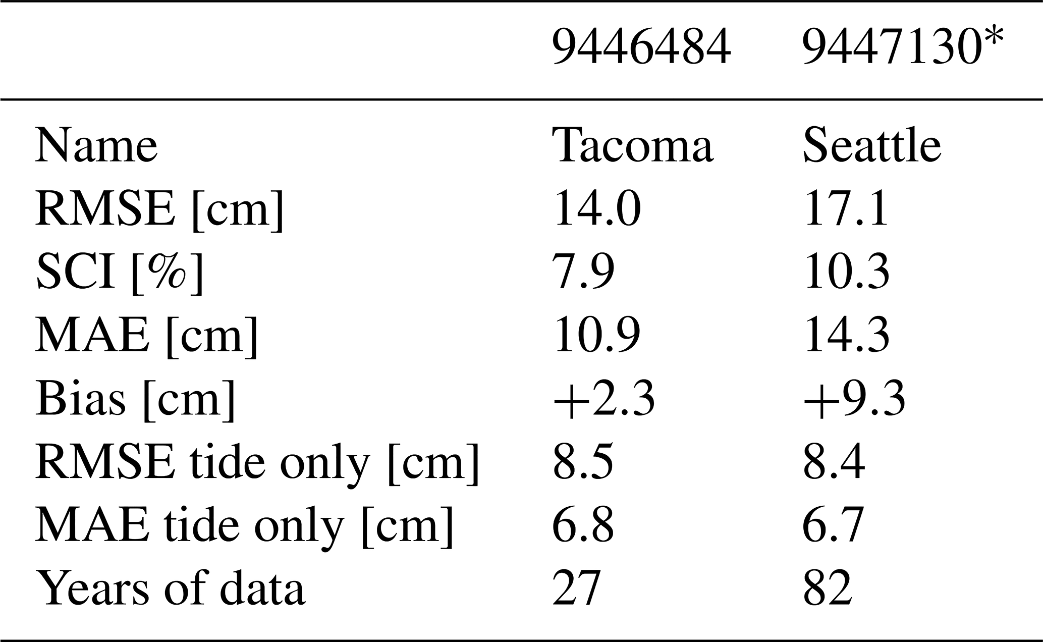
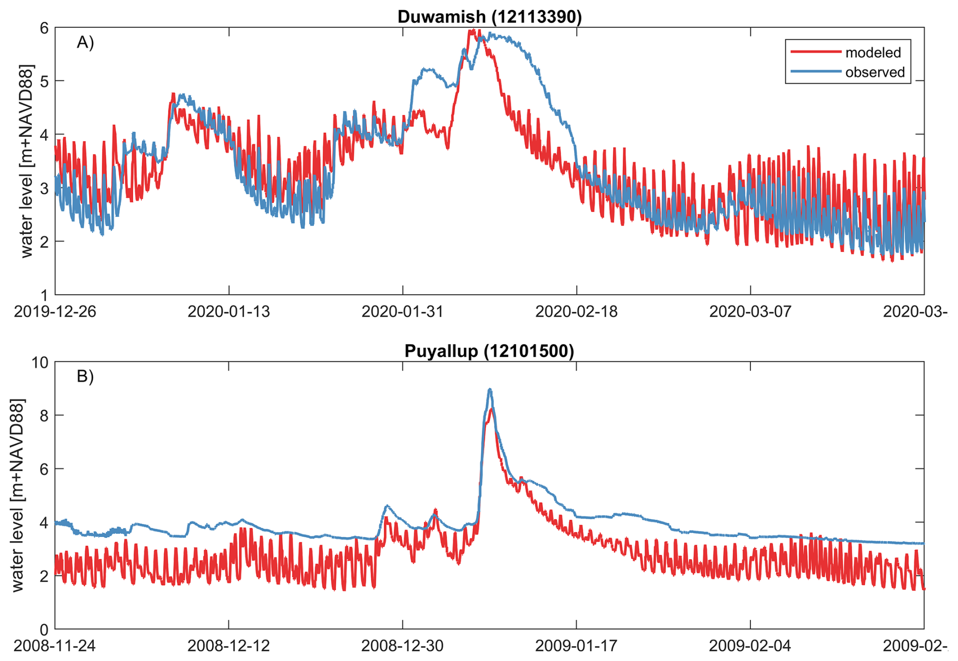
Figure 4 Modeled and observed inland water levels: Panel (A) shows water levels at a streamgage on the Duwamish River (USGS station 12113390), while Panel (B) presents water levels at a streamgage on the Puyallup River (USGS station 12101500; U.S. Geological Survey, 2025).

4.1.2 Inland water levels

Model water levels for October 2007 to the end of WY2022 were validated against gauge data. Two sample time series, each three months long, plot water levels at a streamgage on the Duwamish River (USGS station 12113390; U.S. Geological Survey, 2025) and on the Puyallup River (USGS station 12101500, Fig. 4). Table 2 presents skill scores for five inland water levels across USGS streamgages for which records extended as far back as 15 years. Errors in the model result from a combination of tidal and riverine inflow. The influence of tides appears to be overestimated at both the Duwamish (Fig. 4 – panel A) and the Puyallup (Fig. 4 – panel B) stations. This overestimation is most likely a result of errors in riverine bathymetry, which allow tidal propagation too far upstream. This is apparent from modeling results, where at the Duwamish River USGS station (12113390) tidal oscillations are observed, but their modeled amplitudes are too large. Conversely, at the Puyallup River (USGS station 12101500), tidal effects are not observed, but the model simulates some tidal oscillation. Despite these disparities, the model captures the timing of heightened riverine discharges and associated stage increases. For the Duwamish River (USGS station 12113390), the peak flows are a day early in the model versus observations, while timing at the Puyallup River (USGS station 12101500) is well captured. Errors derived using the uMAE for the gauges range from 37 to 87 cm and represent the combined influence of tidal and riverine error components.

Table 2 Comparison of skill scores for modeled inland water levels at five USGS stations (U.S. Geological Survey, 2025): Performance metrics for modeled water levels are provided for five gauges across the Puyallup and Duwamish watersheds. The number of years of available data for validation is also listed. Stations marked with an asterisk (^*) are reference locations discussed in Fig. 4.

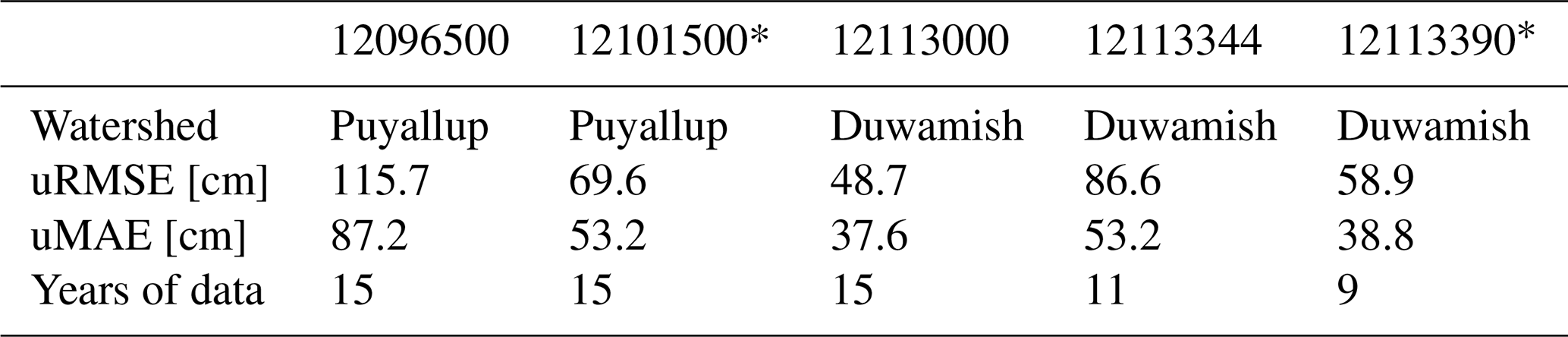
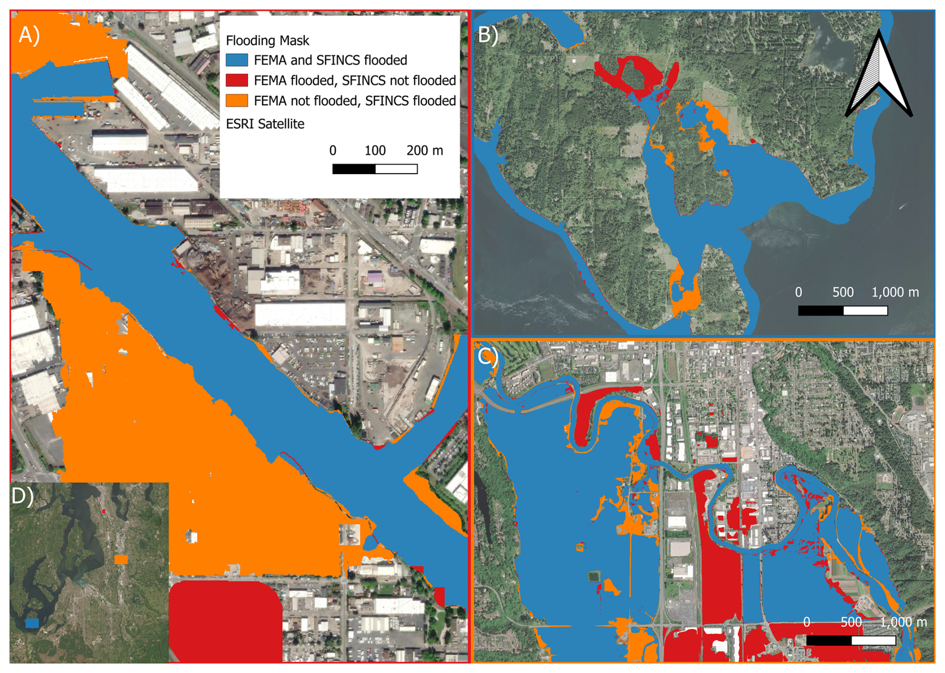
Figure 5 Comparison of 100-year modeled flood extent by SFINCS with FEMA Special Flood Hazard Areas (SFHA) in selected locations across King and Pierce Counties, Washington. Colors represent flood agreement classification: blue for hits (both SFINCS and FEMA indicate flooding), red for misses (flooding observed by FEMA but not captured by SFINCS), and orange for false alarms (SFINCS predicts flooding not identified in FEMA maps). Panel (A) South Park neighborhood in Seattle, WA, adjacent to the Duwamish Waterway. Panel (B) Oro Bay on Anderson Island, WA, illustrates a coastal setting. Panel (C) A reach of the Green/Duwamish River near Kent, WA. Panel (D) overview image. Background: ESRI Satellite Imagery. Sources: Esri, Maxar, GeoEye, i-cubed, USDA FSA, USGS, AEX, Getmapping, Aerogrid, IGN, IGP, swisstopo, and the GIS User Community | Powered by Esri.

4.1.3 Flood extents

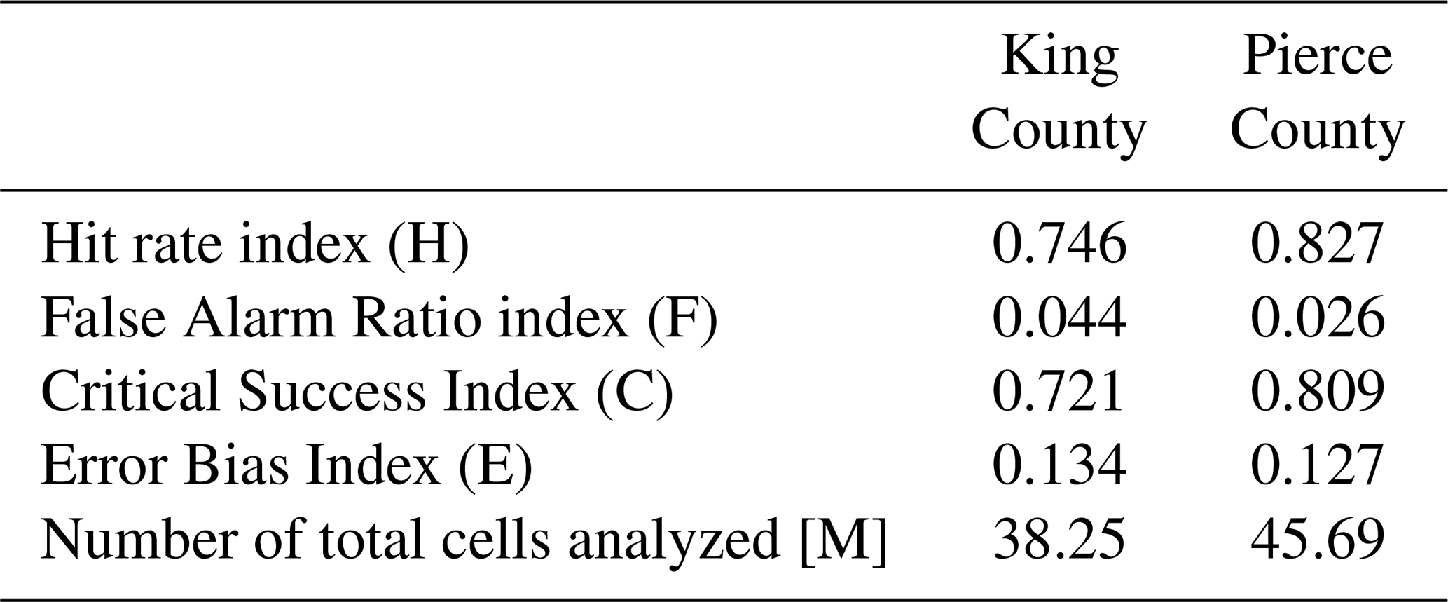
The 2 m resolution flood model was used to determine the 100-year flood extent (1 % AEP) in King and Pierce Counties. The model was compared to FEMA's SFHA, examining 38.25 million grid cells for King County and 45.69 million for Pierce County. The Hit Rate Index (H) was 0.746 for King County and 0.827 for Pierce County, indicating that roughly 80 % of FEMA-mapped flood areas were also identified by the model (Table 3). The Critical Success Index (C), with weight for correct predictions but also weighing misses and false alarms, was narrowly lower (0.721 and 0.809, respectively), indicating minimal false alarms. In particular, the False Alarm Ratio (F) is minimal for each of the counties (0.044 for King and 0.026 for Pierce). The small Error Bias Index reveals that the model underestimates the extent of flooding relative to FEMA maps. Overall, some discrepancies between these two products are expected because the methodologies differ substantially.

Figure 5 demonstrates this performance spatially and highlights the mixed agreement between SFINCS-modeled and FEMA-reported flood extents. Panel A highlights the South Park neighborhood in Seattle, WA, where model results show extensive flooding along the Duwamish Waterway while FEMA maps suggest no flooding despite its history of inundation (refer to Sect. 2 “Study Site”). Panel B shows the Oro Bay coastal region on Anderson Island, WA, where the model and FEMA alignment are mixed, with both areas flooded by SFINCS and not by FEMA, and vice versa. Panel C presents an upstream portion of the Green and Duwamish Rivers near Kent, WA, where both the model and FEMA show strong agreement across a broad river floodplain.

Table 3 Summary of flood extent validation metrics comparing modeled 100-year flood extents with FEMA Special Flood Hazard Areas (SFHA) for King and Pierce Counties. Metrics include the Hit Rate Index (H), False Alarm Ratio (F), Critical Success Index (C), and Error Bias Index (E), based on pixel-level agreement.

4.1.4 Moment of flooding

Unlike traditional flood hazard assessments that rely on predefined design events (e.g., the “100-year flood”), our approach uses the CFRM framework. Both coastal and riverine processes over decades of climate forcing resolve extremes on a grid-cell basis rather than from a single event. Although this approach can complicate communication with stakeholders who are used to the FEMA event-based framework, it provides substantially more robust information about flooding. Retrieval of the exact date and time when peak flooding occurred across space supports validation and analysis of the spatially varying forcing causing the extremes. This approach also provides a spatially robust characterization of extremes. The forcing (and type of event) that causes extremes varies spatially across regions and can be deconstructed. The most natural example of this is the transition from coastally driven to compound to fluvially driven forcing while moving up a river. A single “design storm” modelling approach does not capture this spatial transition in what events are causing extremes.

To support an in-depth analysis of the moment of flooding, a new output variable was introduced into the SFINCS model that records the timestamp of the maximum water level for each grid cell. This new variable enables a spatially explicit assessment of the dominant flood-generating event across the landscape. The resulting analysis is shown in Fig. 6, which maps the peak water levels to specific historical flood events and is summarized in Table 4.

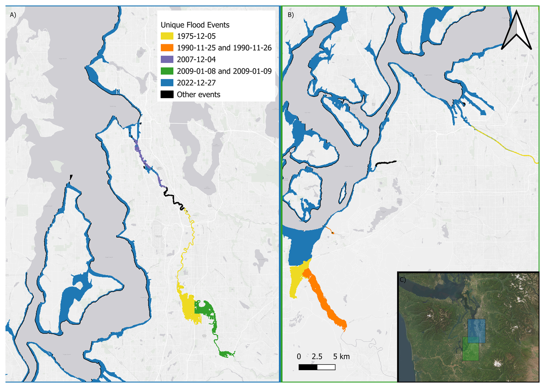
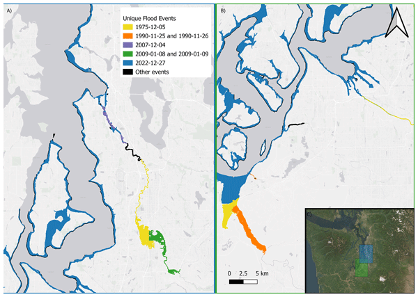
Figure 6 Spatial pattern of individual flood extents as simulated by SFINCS associated with specific historical events in King (A) and Pierce Counties (B), as simulated by SFINCS, and includes an overview map (C). The colors represent the dominant flood event at each location, determined by the peak modeled flood depth timing. The map illustrates the temporal and spatial heterogeneity of flood-generating mechanisms in the region. Background: Esri Gray Canvas basemap. Sources: Esri, HERE, Garmin, FAO, NOAA, USGS, EPA, NPS, and the GIS User Community | Powered by Esri.

An event on 28 December 2022, caused the most widespread flooding in the area. The occurrence was driven by the combined effects of high coastal water levels and high discharge and is colloquially referred to as a “King Tide” event. This King Tide event produced the highest water level for the hindcast period in 78.5 % of King County grid cells and 83.9 % of Pierce County grid cells (blue areas of Fig. 6). One of the most substantial impacts successfully duplicated by the model was on the Duwamish River in Seattle's South Park neighborhood, where business and urban areas were flooded. NOAA tide gauge #9447130 in Seattle recorded water at 3.88 m NAVD88 at 17:00 on 27 December, while SFINCS simulated a high of 4.03 m NAVD88 at 16:20, indicating a close match in amplitude and time. The model also captured other critical events. For example, the event on 8–9 January 2009, led to significant riverine flooding along the Green River, reached a maximum water level in 7.2 % of King County grid cells, and was preceded by warnings of flooding that said the City of Carnation might become an island (KOMO, 2020). There was a local urban flooding incident on 4 December 2007, along the lower Duwamish River, which contributed to 2 % of peak modeled extents in King County. Maximum flooding in 7 % of cells, particularly in the Nisqually River region, occurred during the flood of 25–26 November 1990, in Pierce County. The event, which took place over Thanksgiving week, resulted in two fatalities and involved large-scale evacuations (Hubbard, 1994). The second largest event in the record, based on the number of cells reaching their maximum extent on this date, occurred on 5 December 1975, as a severe winter storm with heavy rain and snowmelt, resulting in widespread riverine flooding within the Green, Nisqually, and Puyallup River systems (STARR, 2015). This 1975 event contributed 10.2 % to the highest modeled water levels in King County and 6.7 % in Pierce County. These events, although less dominant than the 2022 “King Tide” event, demonstrate the diverse mechanisms and regional variation of historical flood drivers in the Pacific Northwest.

Table 4 Summary of the most influential flood-generating events and their areal contribution to peak flood limits in King and Pierce Counties. Percentages refer to the proportion of the total area flooded to which the respective event attained the highest modeled water level. The 28 December 2022, coastal flood event caused the majority of flood extents in both counties, and other events – such as the 1975 Green and Nisqually Rivers flood, and the 2009 upper Green River flood – were more restricted in effect. The rest of the extent was influenced by other, less common events (not shown).

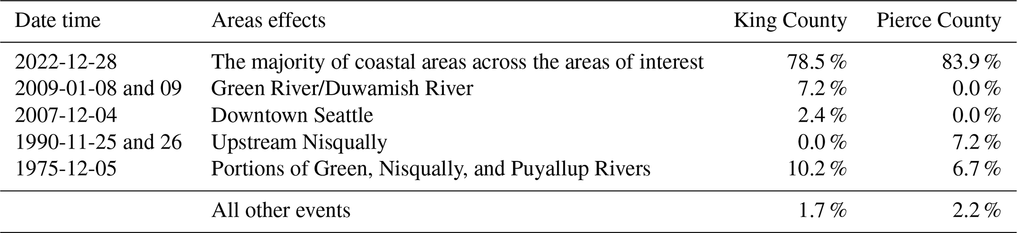
Figure 7 Flooded area (in ha) as a function of return period for three flood severity levels in King County (A) and Pierce County (B) under current climate conditions. Flood severity is classified as severe (red), hazardous (orange), and nuisance (blue). Return periods range from 1 to 100 years, with the final bar labeled EAFA representing the Expected Annual Flooded Area, a probability-weighted integration of flood extents across all return periods. Grid cells that are flooded during daily tidal conditions are removed.

4.2 Flood hazards

4.2.1 Current climate conditions

Flood extents increase consistently with return period in both King County (Fig. 7, panel A) and Pierce County (panel B), illustrating the growing impact of rarer and more intense flood events. In King County, flood extents grow gradually for lower return periods (1 to 10 years), particularly in the severe (red, >1 m depth) and hazardous (orange, >30 cm) categories. For example, severe flooding increases from 9 ha at the 1-year event to 656 ha at 10 years. However, the growth becomes more substantial for higher return periods, especially for nuisance flooding (blue, >10 cm), which reaches 1150 ha at the 100-year event. In Pierce County, total flooded areas are generally larger across all severity levels. Nuisance flooding, for instance, increases from 24 ha (1 year) to 1493 ha (100 years), while severe flooding grows from 13 ha to 931 ha over the same range. The rate of increase slows after moderate events (10–20-year return periods), but flood extent continues to grow with larger return periods, indicating that flood-prone areas are not yet fully saturated.

The final bar in each panel represents the EAFA, a probability-weighted average integrated across return periods from 1 to 100 years. EAFA provides a more holistic and policy-relevant measure of flood hazard, accounting for both event frequency and severity, and is comparable to translating damages to flood risk with the Expected Annual Damages (EAD, Rosbjerg, 2024). In King County, EAFA is estimated at 56 ha for severe flooding, 160 ha for hazardous flooding, and 200 ha for nuisance flooding. In Pierce County, EAFA values are higher with 250, 531, and 644 ha for severe, hazardous, and nuisance flooding, respectively.

The results provided in this subsection so far were computed using the CFRM approach. However, deterministic design events are often used in practice. An example is the simulation of the 10-year flood based on historical storm records. At Seattle (station #9447130), the 5 December 1967, event produced a height of 3.62 m NAVD88 and can be considered the 10-year event based on the Weibull plotting position (Weibull, 1939). When we ran this event through our model and compared the results with the CFRM-based estimate for 10 years, we determined that coastal-zone differences were moderate (simulated high water level at Seattle of 3.72 m NAVD88), giving similar local flood areas. However, further inland along the coastal–riverine boundary, differences grew significantly. Under the deterministic single-event design approach, peak water levels were up to 0.5 m higher in the Duwamish River, flooding a much larger area than under the CFRM method. The mean absolute difference between the two methods was 19 cm and 15 cm, respectively, in King and Pierce Counties. These results demonstrate the importance of the selection of the statistical approach in determining extreme-water-level estimates and, by extension, the spatial extent of flood inundation.

4.2.2 Future climate conditions: sea level rise versus climate change

To evaluate how SLR and future climate conditions influence hazardous flooding (≥30 cm water depth), we analyzed four scenarios: (1) current climate with no SLR, (2) current climate with 1.0 m SLR, (3) future climate with no SLR, and (4) future climate with 1.0 m SLR (Fig. 8). This approach allows isolation of SLR effects vs. climate-change effects. Results are analyzed using the same return periods and the EAFA as in Sect. 4.2.1.

The results indicate that SLR is the dominant driver of increased hazardous flooding. In King County, EAFA increases from 161 ha for the current situation to 787 ha due to 1.0 m of SLR. Similarly, Pierce County shows an increase from 529 to 931 ha. These increases are similar for the 10-year event, which nearly increases fivefold in King County (from 234 to 1241 ha) and increases by more than 50 % in Pierce County (from 913 to 1353 ha). The absolute influence of SLR is particularly pronounced at higher return periods, while the relative increase is largest at lower return periods.

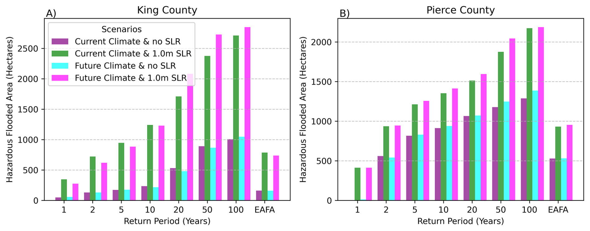
Figure 8 Flooded area (in ha) as a function of return period in King County (A) and Pierce County (B) under 4 different climate and sea level scenarios. Return periods range from 1 to 100 years, with the final bar labeled EAFA representing the Expected Annual Flooded Area – a probability-weighted integration of flood extents across all return periods.

In contrast, future climate forcing alone results in negligible to slightly negative changes in hazardous areas. In both counties, EAFA values stay approximately the same (161 to 160 ha for King County and 529 to 531 ha for Pierce County for current versus future climate, respectively). Moreover, in King County, the 20-year return period hazardous area decreases from 531 to 481 ha (−9 %), while in Pierce County, it increases from 1065 to 1071 ha (+1 %). These results suggest that the future climate conditions modeled (up to 2050) do not intensify but rather slightly reduce flooding. This is an important reminder that climate change (unlike SLR) does not always mean higher flood risk.

When combining both SLR and future climate (Scenario 4, magenta color in Fig. 8), results show only marginal differences from SLR alone (Scenario 2, green color in Fig. 8), reinforcing that SLR is the overwhelming driver of increased hazardous flooding. In King County (Fig. 8A), the EAFA in Scenario 4 is 787 ha, ∼7 % below the EAFA for Scenario 2, which resulted in 738 ha. In Pierce County (Fig. 8B), EAFA increases by ∼2 % (931 ha vs. 954 ha for Scenarios 2 and 4, respectively). Across all modeled return periods, King County shows decreases at lower return periods (−21 % to −1 % for 1–10 years) but increases at higher return periods (+22 % at 20 years and +15 % at 50 years), while Pierce County consistently shows small increases of up to ∼9 %.

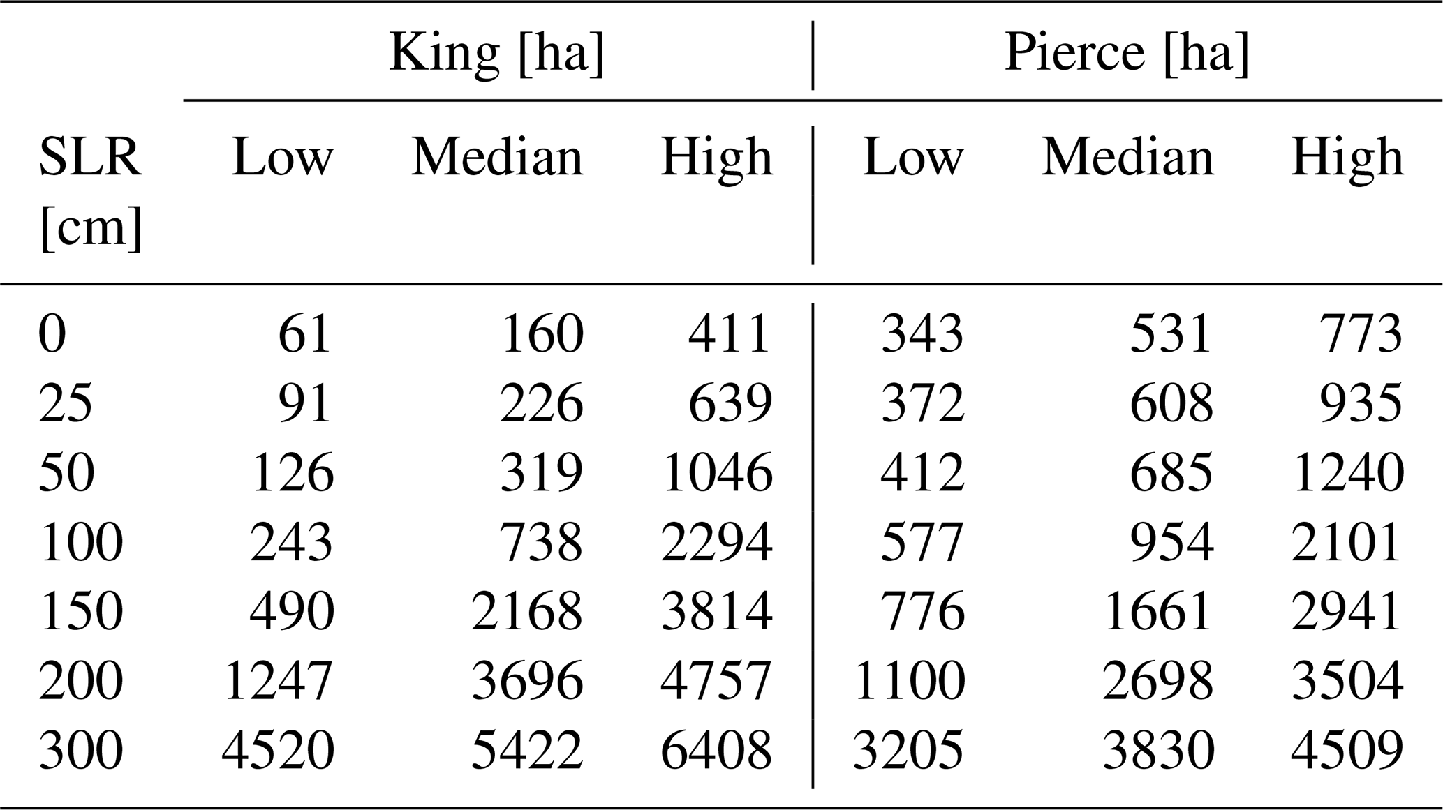
We computed EAFA focused on the hazardous severity class (>30 cm flooding) for King and Pierce Counties as a function of 7 SLR scenarios and accounting for model uncertainty (Table 5). Analysis reveals a threshold in EAFA hazards between roughly 100 and 150 cm of SLR, with median hazards increasing by roughly 13-fold in King County and 3-fold in Pierce County relative to the present-day. This suggests that SLRs exceeding ∼1 m, large new areas of low-lying land (e.g., currently just above the present flood zone) become vulnerable, especially in King County. Hazard increase is gradual below this threshold, but above this threshold, absolute values for EAFA increase steeply. For example, by 300 cm, EAFA ranges from 4520 to 6408 ha in King County and 3205 to 4509 ha in Pierce County. Uncertainty ranges are largest, in absolute terms, at 200 cm SLR for both King and Pierce Counties, while proportionally they peak at 100 cm in King County and 50 cm in Pierce County. These findings demonstrate the model's sensitivity to thresholds. However, at SLR larger than 200 cm, when in absolute terms, uncertainty is large, the proportional spread diminishes, indicating consensus among model scenarios.

Table 5 Hazardous flooding class (>30 cm water depth) Expected Annual Flooded Area (EAFA) for King and Pierce Counties under seven sea level rise (SLR) scenarios. SLR is expressed relative to the mean sea level in 2005 (cm). All EAFA values are in ha (ha). “Low” and “High” represent the lower- and upper-bound estimates from the Low hazard and High hazard uncertainty simulations (refer to Sect. 3.2.2), respectively, while “Median” refers to the central estimate.

5 Discussion

To facilitate reading and ease of understanding, the discussion is divided into five subsections: (1) model performance and validation, (2) benefits of Continuous Flood Response Modeling (CFRM) in determining extremes versus traditional design-event methods; (3) computational trade-offs and limitations; (4) the utility of the Expected Annual Flooded Area (EAFA) metric in planning and risk-informed decision-making; and (5) future directions and adaptation research implications. This organization allows both the methodological improvements and practical applicability of the proposed modeling framework to be considered clearly.

5.1 Model performance and validation

The validation results clearly show that the presented workflow skillfully reproduces coastal water levels (Sect. 4.1.1), inland water levels (Sect. 4.1.2), flood extent (Sect. 4.1.3), and timing of flooding (Sect. 4.1.4). The RMSE errors associated with coastal water levels (14–17 cm) are equivalent to those seen in other regional model studies (Grossman et al., 2023; Nederhoff et al., 2024) and the RMSE error values are greater inland (49–116 cm), primarily due to uncertainty in the riverine bathymetry and an overestimation of tidal propagation, the two limitations of DEMs as they have been hydro-flattened and do not include detailed information about channels. These inaccuracies were further compounded due to sediment accumulation. For example, Czuba et al. (2010) reported sediment accumulation of up to 2.3 m in the lower Puyallup River between 1984 and 2009, with annualized sediment accumulation rates of approximately 13 cm yr⁻¹ in the Nisqually River. As a result, the stage-discharge relationships of streams are inherently non-stationary; therefore, the uncertainty introduced by the stage-discharge relationship when validating model predictions using water levels is independent of model accuracy. This is a common issue with hydrologic modelling, and most regional approaches are validated on discharge rather than water level, as it obscures the lack of information on channel geometry. The primary goal of the framework developed here was to characterize flood hazards, not to reproduce instantaneous water levels, and the high accuracy of the FEMA flood extent maps (hit rates 0.75–0.83) indicates that it is reliable for characterizing flood hazards. Strong model performance is attributable to (1) the nesting of the overland flow domains within large-scale coastal and inland models that provide reliable boundary conditions and (2) the inclusion of relevant bathymetric features. Computational efficiency was a key design consideration to enable the usage of the CFRM framework and simulation of thousands of years (i.e., 7+2 SLR scenarios, 3 uncertainty layers, 2 domains, 100 years =5400 simulations) of hydrodynamic processes. However, this consideration came with trade-offs: the model resolution was constrained to 50×50 m, with fine-scale flood features resolved using subgrid lookup tables based on a 1 m DEM. We acknowledge that this tradeoff sacrifices, to some degree, the accuracy with which water levels are simulated (as gauged in the validation) for better fidelity in extremes and compound events. For example, one week of simulation at very high resolution and with a full physics model would produce better validation statistics, but at the cost of requiring an event-based strategy that sacrifices fidelity in description of the extremes. This loss of accuracy (decreased power to statistically capture extremes) is harder to quantify but must be considered in the choice of a specific workflow. Additionally, the explicit quantification of uncertainty through low and high boundary condition simulations (Sect. 3.4) provides stakeholders with a realistic envelope of potential flood outcomes.

5.2 Benefits of Continuous Flood Response Modeling (CFRM) for extreme events

From an extreme value analysis (EVA) perspective, the chosen approach provides important advantages. The first is that a continuous 100-year simulation approach enables a cell-by-cell empirical EVA without requiring the fitting of statistical distributions. Fitting of an EVA statistical model adds significant uncertainty to predicted extremes, and an EVA model (statistical in nature) will underperform relative to a physics-informed model at constraining extremes. Second, abandoning the traditional application of a single, one-off “100-year” design event is particularly warranted in dynamic coast–riverine settings where diverse combinations of drivers can produce equally hazardous, yet spatially distinct, flood effects. As shown in Fig. 6, a succession of diverse storms contributed importantly to the historical flood record, so a single, representative “100-year event” might mistakenly identify vulnerable areas. Our comparison in Sect. 4.2.1 also makes the point that deterministic 10-year design events produced local flood levels that were locally as much as 0.5 m higher than the CFRM-derived 10-year estimate, demonstrating how extreme water levels and flood extents depend on the method used to derive them. Finally, the continuous time-series approach naturally captures compound extreme events where coastal and river forcings are phase-lagged or decoupled, for example, a coastal surge with a peak days apart from a river flood would most likely be underestimated by one design storm. As a result, CFRM provides a robust and spatially representative basis for flood hazard assessment and planning.

Secondly, traditional design events, typically represented by a single, static, deterministic “100-year” scenario, may not effectively model dynamic coastal–riverine systems where multiple drivers can produce diverse flood outcomes. As illustrated in Fig. 6, several distinct storms contributed significantly to the historical flood record. Modeling the region with a single design event would therefore underpredict extremes at some locations where the incorrect 100-year storm is being modeled. In particular, the difference between the CFRM and the deterministic 10-year design event revealed a MAE of ∼19 cm with local differences as high as 0.5 m (Sect. 4.2.1). Additionally, a continuous time-series approach improves consideration of compound extreme events where fluvial and coastal side forcing may be phase-lagged or even decoupled.

5.3 Limitations and computational trade-offs

The chosen model configuration reproduces flooding well across most of the domain, achieving high spatial agreement with FEMA flood extents (hit rates: 0.75–0.83). However, in narrow rivers, the model introduces localized edge effects that result in overestimation of the river footprint. These effects are driven by the relatively coarse modeling resolution in combination with the usage of weirs. However, these limitations are consistent with other subgrid modeling approaches (e.g., van Ormondt et al., 2025a). Incorporating subgrid bathymetry is rapidly becoming the new standard because it allows the user to account for more information per grid cell and therefore improves the accuracy of the simulation. Subgrid bathymetry refers to storing and using high-resolution elevation information (e.g., 1 m DEM data) inside each larger model grid cell (e.g., 50 m) and allows the user to simulate on coarser resolutions without significant loss of accuracy. Coastal boundary mismatches are within the range of previous efforts (e.g., Nederhoff et al., 2024), driven by both differences in tides and the NTR. The persistent bias at Seattle (#9447130) is notable and is hypothesized to result from steric density-driven effects that are not accurately captured by the regional model (Parker et al., 2026). Inland water level offsets stem from uncertainties in total inflow estimates (Buitink et al., 2026) and inaccurate riverine bathymetry. In some cases, bathymetry was manually deepened to improve hydraulic connectivity (refer to Sect. 3.2). Good-quality bathymetric data at the riverine–coastal interface remains a challenge over much of the globe, despite this interface being one of the most vulnerable regions to SLR and climate-driven change.

Simplifications in the model and assumptions were required by computational and scale constraints. The SFINCS model used in this study has no stationary wave solver, infragravity waves, rainfall-runoff processes, sediment transport, or morphological change. Also, the SFINCS domains were not calibrated; default parameter values were used throughout. Future calibration of parameters such as bottom friction could improve model accuracy. Wave setup was prescribed at the offshore boundary using a simple estimate of 20 % of the wave height, similar to Vousdoukas et al. (2018). Sensitivity testing of different values to translate wave height to sustained setup from 0 % to 20 % (e.g., Feng et al., 2011; Yamanaka et al., 2020) demonstrates limited influence on flood extents. In particular, using a constant value 5 % instead of 20 % decreased the EAFA for hazardous flooding for King and Pierce County, from 160 and 644 to 91 and 400 ha, respectively (84 %–14 % change). Observations of wave setup in low wave energy environments are sparse, and a case study with more comprehensive data at the exposed shoreline could provide further insights. High-fidelity wave-resolving modeling of overtopping and runup was deemed too computationally expensive, especially with the inherent uncertainties of wave processes in the Puget Sound environment. The absence of these processes, as well as detailed rainfall runoff modeling, likely leads to the underestimation of flood hazards in both coastal and inland zones. A comparison with FEMA 100-year flood maps yielded hit rates between 0.75 and 0.83, though the bias index (0.13) indicates a tendency to underpredict flood extent.

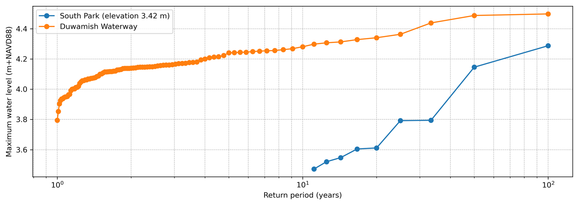
Figure 9 Empirical return period curves for the Duwamish Waterway (channel) and South Park (floodplain). Channel water levels follow smooth extreme value behavior suitable for distribution fitting, while floodplain response exhibits threshold-dependent activation. The different curve shapes and offsets demonstrate limitations of extrapolating fitted channel distributions to predict overland flood hazard.

While the CFRM approach was chosen for its multiple advantages, it is important to note that we simulated only 100 years of hydrodynamic forcing; therefore, by definition, the maximum flood extent observed corresponds to the 100-year event. This relatively low number of simulated years restricts the statistical confidence within the higher end of the extreme value frequency and does not identify rarer combinations. However, the usage of the Weibull plotting position eliminates the need to fit a distribution and results in a more robust extreme value estimate. For example, Fig. 9 presents the model output at the Duwamish Waterway, which has a smoothly shaped empirical distribution that can be fitted with either a GEV or GPD model. However, the flood response of the floodplain at South Park has threshold-dependent characteristics and is only flooded when T exceeds ∼10 years. Extreme Value Analysis requires maxima from a stationary distribution, and the changing elevation difference between the water level in the channel and on land, plus fundamentally different shape characteristics, violate this assumption. With the statistical underpinnings of EVA undermined, it is challenging to have confidence in predictions of overland flood hazards based on extrapolations from channel gauge readings. CFRM maintains the physical discontinuities in levee overtopping thresholds and backwater effects, which would be smoothed out by parametric distributions. Extending the length of the simulation would reduce the uncertainty of the higher return period estimates and allow for a more comprehensive sampling of tidal and storm interactions. The length of the simulation was not increased in the present study due to computational cost constraints, which remain a limit on long-duration, high-resolution flood simulation. However, this framework permits temporal analysis of flooding, which can be used for validation (Sect. 4.1.4) and planning.

5.4 Expected Annual Flooded Area (EAFA) and planning relevance

Expected Annual Flooded Area (EAFA), or “probability-weighted” flooded area, is an improved metric to assess the contribution of floods through all possible return periods. EAFA is a superior metric for planners than a fixed frequency flooded area since it represents a scalable and continuous measure of flood hazard. Further, there is a growing agreement that deterministic flood maps, although useful for regulatory purposes, are insufficient for climate-informed planning (Wing et al., 2022). Binary discretised results (flooded or not flooded) for a single storm do not portray the gradient of risk over return periods or the probabilistic nature of flooding. EAFA avoids these restrictions by providing a scalable, continuous depiction of flood hazard that is better adapted for cost-benefit analysis and resilience planning.

Use of EAFA to estimate spatial flood extent is conceptually equivalent to the Expected Annual Damage (EAD) used in economic risk assessment by agencies such as FEMA (Rosbjerg, 2024) to estimate financial damages and is starting to be used more frequently (e.g., Vousdoukas et al., 2023). However, by merging EAFA with exposure layers, spatial patterns of expected annual impact can be estimated. This synthesis can enable agencies and municipalities to identify high-hazard areas, rank adaptation investments, and evaluate the performance of proposed interventions over time. EAFA is not meant to substitute but to supplement and enrich the planning and readiness of the community. Incorporation of EAFA in long-term planning reports, climate change adaptation plans, and capital investment plans can transform flood management from event-based, static models to response-based, dynamic risk management.

5.5 Future research and adaptation implications

Although this paper considers future flood risk due to climate change and sea level rise (SLR) scenarios, it does not consider morphological change (e.g., shoreline and bluff retreat) or societal growth (e.g., increased population, new infrastructure). Both systems are likely to evolve dynamically in response to these drivers. For example, shoreline and bluff retreat are projected to occur in many locations under increasing sea levels (Vitousek et al., 2017). Similarly, the built environment will also adapt to changing hazards, and therefore, the likelihood of repeated flooding will be influenced by the adaptive measures implemented by communities responding to the evolving natural system.

Our findings indicate that SLR is a much more significant driver of future flood hazard in King and Pierce Counties than other climate change-related factors, such as changes in storm patterns, for the period assessed (through 2050 using the HighResMIP climate ensemble). Somewhat counterintuitively, the simulations show reduced flooding under future climate forcing alone without SLR. For this study, projected climate changes were derived using a cumulative distribution function (CDF) correction applied to the ensemble mean of 7 high-resolution CMIP6 models, following Parker et al. (2026). The relatively subdued or even negative storminess-driven changes in EAFA and return period flood extent under future climate forcing (in the absence of SLR) must be interpreted in the context of both methodological and climate-signal considerations. Similar patterns were observed when assessing projected changes in storm surge and wave climate around the Salish Sea using the same seven-member HighResMIP CMIP6 ensemble (Parker et al., 2026). High spread among individual CMIP6 members was noted, with several models producing consistently smaller changes than the others; when averaged, these model results weakened the ensemble-mean signal. This high model variability suggests that the ensemble mean may underestimate potential changes captured by some members. A second important point is the time-horizon mismatch between the climate-change and SLR scenarios used here. The HighResMIP CMIP6 simulations represent potential effects until 2050, whereas our SLR scenarios may represent longer-term futures. As a consequence, the relative magnitude of storminess change and SLR is not directly comparable. These findings underscore the importance of caution in interpreting ensemble-mean climate change effects on extremes in the Salish Sea, at least when confined to mid-century time frames. Longer-term, high-resolution climate forcing data sets – considering both hydrologic and oceanographic inputs – would be required to directly compare century-scale SLR projections with storminess change on the same time scales.

Further modelling efforts could include physical processes not simulated here, such as wave runup and rainfall-runoff routing. Higher spatial resolution and more accurate representation of hydrologic and land-sea interaction processes could enhance model fidelity, particularly in compound flood settings. A more detailed representation of urban drainage infrastructure and dynamic groundwater-surface water interactions would be needed for more complete inland flood simulations. Finally, combining EAFA or other hazard metrics with dynamic exposure layers (population, assets, critical infrastructure, etc.) would aid in the development of actionable, risk-based adaptation plans.

6 Conclusions

This study addressed growing flood risk in a relatively steep coastal estuarine system in the Pacific Northwest, where sea level rise and changing storm systems threaten coastal and riverine communities and regionally important infrastructure. Traditional flood estimations with design events (e.g., FEMA's 100-year flood) are challenged to accurately represent the compound and spatially varying nature of extreme water levels. In an attempt to overcome this limitation, we utilized a Continuous Flood Response Modeling (CFRM) approach to simulate overland flooding in Pierce and King Counties using high-resolution SFINCS models. The approach incorporated many decades' worth of dynamic boundary forcing data (coastal water levels and riverine inflow), and spatially variable friction, bathymetry, land cover, and topography to simulate dynamic flood processes. This approach enabled empirical determination of extreme recurrence at per-cell resolution sensitive to the combined effect of coastal and fluvial forcing and independent of statistical assumptions. Furthermore, the inclusion of a new innovative variable in SFINCS allowed accurate tracing of the timing of peak water levels, offering insights into dominant flood-generating events both spatially and temporally, and offering additional opportunities for validation.

Validation showed model performance of simulating coastal water levels with errors of 14 to 17 cm at two NOAA gauges and inland water levels with RMSEs of 49–116 cm at five USGS streamgages. Agreement with FEMA flood maps was high (hit rate indices of 0.75 in King County, 0.83 in Pierce County) with a slight underestimation bias (error bias index ≈ 0.13).

Under current climate conditions, the model predicted substantial spatial variation in flood hazards. The Expected Annual Flooded Area (EAFA), a probability-weighted sum of all return periods, ranged from 56 to 200 ha in King County and 250 to 644 ha in Pierce County based on flood severity. Modeled future climate conditions showed that SLR is the dominant variable causing increased flood extent, while simulated climate forcing changes without SLR had negligible or even slightly negative effects on the area flooded. One important observation in these runs is the presence of a threshold in the relationship between SLR and flood risk. Particularly, we detected the largest increases in flood risk between 100 and 150 cm SLR. The analysis also revealed that accounting for all relevant drivers (tide, surge, discharge) is essential for accurately predicting flood risk. A simplified, deterministic mapping approach based on a 10-year design flood resulted in flood depth errors of up to 0.5 m and significantly different spatial extents.

These findings demonstrate the utility of CFRM in flood risk estimation. Furthermore, EAFA provides a quantitative and informative index to planners and policymakers, offering a more complete evaluation of flood risk, including probability, than traditional single–return-period flood maps. Future research could incorporate other drivers, such as direct rainfall and wave behavior, and integrate flood hazard projections with exposure and vulnerability data to fully express risk.