Predicting spatio-temporal wildfire propagation with dynamic firebreaks

Wildfire management strategies increasingly demand accurate predictive models that integrate real-time intervention measures. Despite advances in machine learning (ML) for wildfire modelling, existing approaches largely overlook the role of firebreak placement. In this work, we present the first deep learning-based predictive model for simulating spatio-temporal wildfire propagation with dynamic firebreaks. Utilizing a Convolutional Long Short-Term Memory (ConvLSTM) architecture, the model captures both the spatial and temporal complexities of wildfire spread while incorporating data on firebreak positioning and effectiveness. Our training dataset, derived from Cellular Automata (CA) simulations, integrates key geophysical parameters and human intervention strategies, including temporary and permanent firebreaks. Model validation across three major wildfire events in California demonstrates robust performance, with significant accuracy gains in scenarios involving strategic firebreak placement. This integration of movable firebreak placement into a wildfire spread model provides a tool for improving real-time wildfire management efforts.

1 Introduction

In recent years, extreme fires have become more frequent, driven by ongoing climate change (UNEP, 2023; Cunningham et al., 2024). There is a growing literature on management strategies to prevent or minimise fires (Spadoni et al., 2023; Oliveras et al., 2025; Neidermeier et al., 2023). However, it is also important to develop effective strategies to reduce the impact of fires when they occur. One measure that is frequently used is the creation of temporary firebreaks, through the use of fire retardants (Gimenez et al., 2004; Altamimi et al., 2022; Goldberg, 2022). The effectiveness of such a measure is substantially affected by uncertainties in the propagation of an individual fire caused by short-term variability in both meteorological conditions and fire behaviour (Hilton et al., 2015). Thus, the accurate prediction of fire spread in near-real time and how this would be affected by potential management actions would be a useful tool for proactive fire reduction.

In recent years, machine learning (ML) techniques have gained significant attention in the analysis of dynamic systems, particularly in wildfire prediction (Jain et al., 2020; Xu et al., 2025). These techniques are recognized as invaluable tools for spatio-temporal forecasting due to their ability to efficiently process large datasets and uncover complex patterns within historical data. Various approaches have been explored in wildfire modelling, such as convolutional autoencoders (Huot et al., 2022; Cheng et al., 2022a), recurrent neural networks (RNNs) (Natekar et al., 2021; Cheng et al., 2022b), and, more recently, transformer-based models (Miao et al., 2023; Masrur et al., 2024). Given the inherent temporal dynamics of wildfire spread, Long Short-Term Memory (LSTM) networks – an advanced form of RNN designed to capture time-sequential patterns – have been widely used to model the progression of fire over time (Cheng et al., 2022b; Liu et al., 2022; Liang et al., 2019; Natekar et al., 2021). In particular, Kondylatos et al. (2022) have shown that deep learning (DL) techniques, including LSTM and Convolutional Long Short-Term Memory (ConvLSTM), are more effective than shallow ML methods like Random Forest and XGBoost in predicting wildfires in the Mediterranean region. While incorporating advanced RNN architectures significantly enhances predictive accuracy in wildfire modelling, the integration of human actions in these models requires further exploration.

Despite significant advances in ML models and the availability of numerous open-access benchmarking datasets (Huot et al., 2022; Kondylatos et al., 2023; Singla et al., 2021) for performance evaluation, no existing ML predictive or surrogate model explicitly addresses the impact of real-time firebreak placement. Mutthulakshmi et al. (2020) outline two main firefighting strategies: temporary holding firebreaks (e.g., water or chemical firebreaks deployed by aircraft) and permanent firebreaks (e.g., cleared or fuel-poor areas constructed using machinery) and emphasizes that the strategic positioning and selection of firebreaks can optimize the management of the burning area. Experimental findings from Alexandridis et al. (2011) show that the number of burning cells can be decreased by 56 % with adequate resources. However, simulating fire propagation with suppression, given the complexity of geophysical parameters, presents a substantial computational challenge. The high computational costs often prevent real-time prediction, which is essential for timely intervention. The Mutthulakshmi et al. (2020) fire-suppression model using Cellular Automata (CA), for example, simulates fire spread with human interventions but has significant memory and time demands – especially for large areas – which limits its usefulness. Similarly, the Discrete Event System Specification (DEVS) (Ntaimo et al., 2004) struggles to meet real-time requirements when updating fire parameters based on previous states. Recent work (e.g., Murray et al., 2024; Altamimi et al., 2022) has used reinforcement learning for optimal firebreak placement. Pan et al. (2024) presents a framework that integrates convex neural network-based fire spread prediction with optimization methods to coordinate drone swarms for active wildfire suppression. Meng et al. (2023) introduces a 3D visualization approach based on CA for simulating fire spread with the inclusion of temporal firebreaks. However, the forward predictive models in these approaches are often simulation-based, which limits them to somewhat simplified wildfire scenarios due to computational costs.

In this paper, we develop a computationally efficient fire propagation surrogate model that accounts for both permanent and temporary firebreaks. Using a CA framework, we simulate fire dynamics under various environmental conditions across three wildfire-affected locations. The model incorporates firebreak data along with local geophysical parameters such as vegetation, slope, and wind speed. We then train a DL surrogate model based on the ConvLSTM algorithm to predict fire spread. The model is validated using test data from the CA simulations. It is important to emphasize that the present study is intended as a proof of concept demonstrating that a ConvLSTM-based surrogate model can successfully learn wildfire spread dynamics with dynamic firebreak deployment. The objective is methodological validation rather than the development of a fully operational forecasting system. While wind and landscape variability are critical drivers of real wildfire behaviour, incorporating fully dynamic, high-resolution environmental forcing would substantially increase the dimensionality of the training space and require the generation of a significantly larger number of CA simulations. The proposed framework is flexible and can be extended in future work by enriching the training dataset with diverse wind directions, gust dynamics, and additional environmental drivers, thereby enabling the model to learn sensitivity to these factors and improving its applicability to more realistic operational settings.

2 Data and Methods

Maps for each of the study areas were processed using remote sensing images of the Moderate Resolution Imaging Spectroradiometer (MODIS) and Visible Infrared Imaging Radiometer Suite (VIIRS) satellite which are available at the Interagency Fuel Treatment Decision Support System (IFTDSS) (Drury et al., 2016). We used three wildfire events in California: the “Chimney” fire in 2016 (Chimney 2016)¹, the “Ferguson” fire in 2018 (Ferguson 2018)², and the “Bear” fire in 2020 (Bear 2020)³ (Fig. 1).

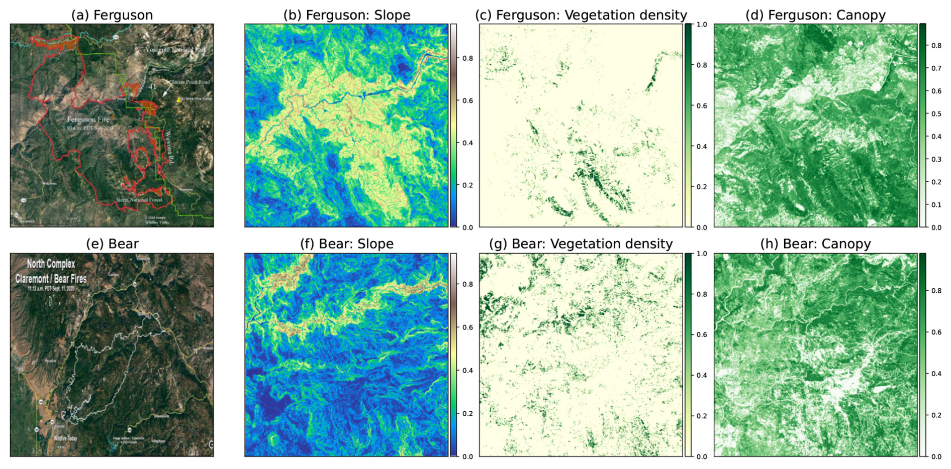
Figure 1 The Ferguson 2018 fire landscape presents normalized data in slope, vegetation density, and canopy cover (a, b, c, d). Similarly, the Bear 2020 fire depicts distinct topographical and ecological normalized data, including slope, vegetation density, and canopy distribution (e, f, g, h). Panel (a) shows the perimeter of the Ferguson Fire at 01:30 PDT on 4 August 2018. Map data ©2018 Google; reproduced from Wildfire Today (2018). Panel (e) shows North Complex Claremont/Bear fires at 11:12 PDT on 11 September 2020. Image Landsat/Copernicus; map data ©2020 Google; reproduced from Wildfire Today (2020).

Figure 2 provides an overview of the data generation, model training, and prediction workflow used in this study. First, a CA simulator is employed to generate spatio-temporal wildfire propagation data under various environmental conditions and firebreak deployment scenarios. These CA-generated fire spread sequences, together with firebreak information, are then used to train a ConvLSTM-based surrogate model. During inference, the trained ConvLSTM model takes a sequence of previous fire states as input and predicts subsequent wildfire evolution with significantly reduced computational cost. This workflow illustrates the relationship between the physics-inspired CA simulator and the data-driven ConvLSTM model, and clarifies how the two components are integrated in the proposed framework.

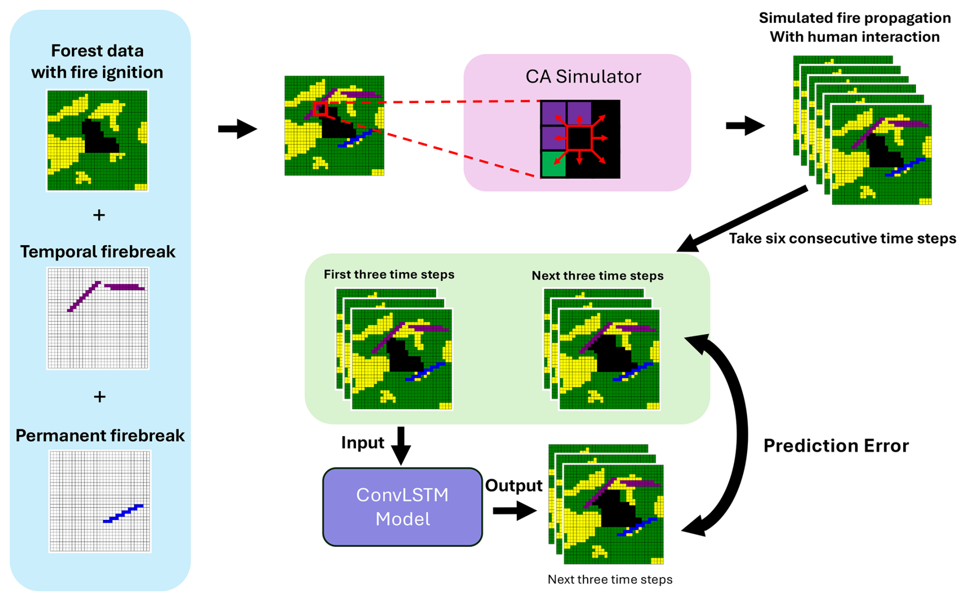
Figure 2 Workflow of the proposed framework, illustrating CA-based data generation, ConvLSTM model training, and surrogate wildfire prediction.

2.1 Cellular Automata Fire Simulation

We build upon the CA model that was validated through the simulation of the Spetses wildfire in Greece in 1990 (Alexandridis et al., 2008), to generate the data sets used for training and testing our DL surrogate model. This CA model utilizes square meshes to simulate the stochastic spatial spread of wildfires in a computationally efficient way. By dividing a two-dimensional terrain into 3 × 3 grids, the model allows fire propagation in eight possible directions determined by evaluating the state of a central cell based on the states of its neighbouring cells (Alexandridis et al., 2011). The accuracy of the model when fire suppression strategies were included was validated by using the 2014 Dumai forest fire over a 14 d period (Mutthulakshmi et al., 2020).

Our CA model incorporates local environmental parameters such as forest information, vegetation density, slope, and meteorological data such as wind speed and wind direction to simulate fire dynamics. Training datasets were derived from three recent fires in California. Various firebreak placement scenarios were evaluated to assess their impact on fire spread. Specifically, we implemented new states in the CA model to represent permanent and temporary firebreaks. For temporary firebreaks, we developed an approach that encodes their remaining duration, allowing the model to track their effectiveness over time. The states of each cell within the grid evolve through discrete time steps as follows:

• State 1. The cell contains no fuel and cannot burn.

• State 2. The cell contains fuel but has not yet ignited.

• State 3. The cell contains fuel and is actively burning.

• State 4. The cell has burned out and can no longer ignite.

• State 5. The cell is part of a permanent firebreak.

• States 15 → 6. The cell is part of a temporary firebreak that will transit from state 15 to state 6 over 10 time steps, before reverting to its original state.

The transition between CA states evolves over time (Fig. 3), and the cells that are either non-burnable (State 1) or have already burned (State 4) do not change state. Burnable cells (State 2) have a probability P_burn of igniting if one or more of their neighbouring cells are burning. Fire spreads to adjacent cells through stochastic transitions from State 2 to State 3, with the ignition probability determined by a probabilistic rule defined in Eq. (1):

$$\begin{array}{}\text{(1)}& P_{\mathrm{burn}}=p_h\left(\mathrm{1}+p_{\mathrm{veg}}\right)\left(\mathrm{1}+p_{\mathrm{den}}\right)p_{\mathrm{s}}{p}_{\mathrm{w}},\end{array}$$

where p_h denotes the base burning probability, while p_veg, p_den, p_s, and p_w correspond to local environmental factors such as vegetation density, canopy cover, slope, wind speed and wind direction, respectively. These parameters are sourced from the IFTDSS (Drury et al., 2016). The influence of slope on fire spread is modelled following Weise and Biging (1997), with the slope effect p_s given as:

$$\begin{array}{}\text{(2)}& p_{\mathrm{s}}=\exp \left(a{\mathit{\theta }}_{\mathrm{s}}\right),\end{array}$$

where a is a dimensionless constant, and the slope angle θ_s is calculated using the following expressions:

$$\begin{array}{}\text{(3)}& {\mathit{\theta }}_{\mathrm{s}}=\left\{\begin{array}{ll}{\tan }^{-\mathrm{1}}\left(\frac{E_{\mathrm{1}}-E_{\mathrm{2}}}{l}\right),& \text{for adjacent cells}\\ {\tan }^{-\mathrm{1}}\left({\displaystyle \frac{E_{\mathrm{1}}-E_{\mathrm{2}}}{\sqrt{\mathrm{2}}l}}\right),& \text{for diagonal cells}\end{array}\right.\end{array}$$

Here, E₁ and E₂ denote the elevations of the respective cells, and l represents the cell length. The wind effect is modelled following the method proposed in Alexandridis et al. (2008), where:

$$\begin{array}{}\text{(4)}& p_{\mathrm{w}}=\exp \left(c_{\mathrm{1}}{V}_{\mathrm{w}}\right)\exp \left(V_{\mathrm{w}}{c}_{\mathrm{2}}\left(\cos \left({\mathit{\theta }}_{\mathrm{w}}\right)-\mathrm{1}\right)\right).\end{array}$$

V_w represents the wind speed in meters per second, and θ_w is the angle between the wind direction and the potential fire spread direction (Eq. 4). The coefficients c₁ and c₂ are tunable parameters that modulate the wind's effect on fire propagation (Alexandridis et al., 2008). Wind data, including both speed and direction, were taken from Hersbach et al. (2020). Wind conditions were assumed to be spatially constant over a 27 km × 27 km grid, and the burned area state were resized to 128 × 128 pixels. Each CA simulation time step corresponds to approximately 6 h (Cheng et al., 2022b). This simplification was adopted to constrain the dimensionality of the training space in this proof-of-concept study.

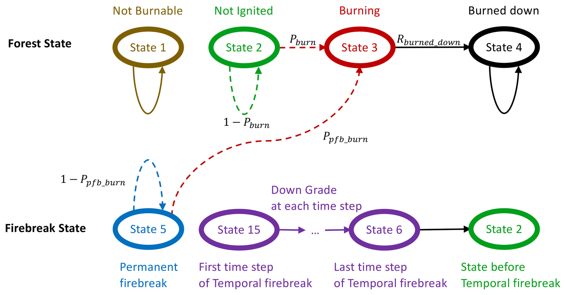
Figure 3 State transition pipeline of the CA model when a neighbouring cell is burning. Solid arrows denote deterministic state transitions, while dotted arrows indicate probabilistic transitions, with the associated probabilities shown next to each arrow. Non-burnable cells (State 1) remain unchanged. Burnable but unignited cells (State 2) ignite with probability P_burn and transition to the burning state (State 3) when one or more neighbouring cells are burning. Burning cells (State 3) transition to the burned-out state (State 4) with probability R_{burned_down}. Cells within permanent firebreaks (State 5) may still ignite with probability P_{pfb_burn}. Temporary firebreaks are initialized at State 15 upon deployment and deterministically degrade by one state at each subsequent time step, transitioning from State 15 to State 6 over 10 time steps, after which the cell reverts to its original pre-firebreak state.

The operational parameters p_h, a, c₁, and c₂ significantly influence fire spread predictions. In Alexandridis et al. (2008), these values are calibrated as follows:

$$p_h=\mathrm{0.58},a=\mathrm{0.078},c_{\mathrm{1}}=\mathrm{0.045},c_{\mathrm{2}}=\mathrm{0.131}.$$

These values are derived by minimizing a cost function that fits observed fire spread data from specific wildfire events, and are used as initial values in the parameter identification process. Finally, burning cells (State 3) transit to a burned state (State 4) with a fixed probability R_{burned_down} = 0.4 throughout the entire simulation.

Our CA model incorporates both temporary and permanent firebreaks. Temporary firebreaks are flexible in their placement and provide complete fire suppression for a limited duration of 10 time steps, equivalent to approximately 3 d (with each time step representing 6 h in real time). In contrast, permanent firebreaks require a minimum distance of 1 km (equivalent to 5 pixels in the CA model) from the fire front and offer a suppression rate of about 90 % (Plucinski et al., 2007). Both types of firebreaks are subject to resource constraints, limiting their maximum extent (in our model that is limited to 50 pixels for each type of firebreak).

For cells affected by a permanent firebreak (State 5), the suppression rate (R_pfb) is 90 %. The probability that a cell under the influence of a permanent firebreak will still burn, P_{pfb_burn}, is given by:

$$\begin{array}{}\text{(5)}& P_{\mathrm{pfb}\mathrm{\_}\mathrm{burn}}=\left(\mathrm{1}-R_{\mathrm{pfb}}\right)P_{\mathrm{burn}},\end{array}$$

where P_burn is the standard burning probability, calculated using Eq. (1).

Temporary firebreaks (States 15 to 6) are assumed to provide 100 % fire suppression for an effective period of approximately 3 d. In the CA simulator, these temporary firebreaks provide complete (100 %) suppression throughout their effective duration of 10 time steps, after which they revert to their original state, allowing fire spread to resume if conditions permit.

The training data set generated by the CA simulator (Fig. 4) uses data from each landscape: “Chimney 2016”, “Ferguson 2018”, and “Bear 2020”. Each dataset was generated with random wind directions, randomly positioned fire ignition field, three temporal firebreaks and one permanent firebreak positioned around the ignition field and the CA model simulates fire propagation for 26 time steps, approximately 7 d in real time. Firefighting strategies typically involve placing firebreaks along the active fire front to slow or stop the spread. However, due to the unpredictable and often rapid progression of wildfires, it is not always possible to deploy firebreaks in optimal locations. In our study, we used randomly positioned firebreaks to evaluate whether the DL model can still accurately predict fire propagation under less controlled conditions.

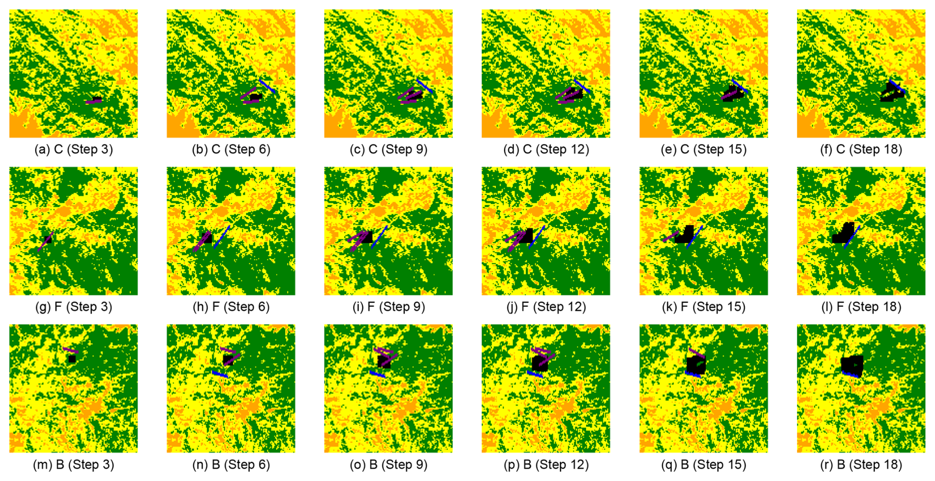
Figure 4 The fire propagation simulation of 16 time steps using CA on C (“Chimney 2016”), F (“Ferguson 2018”) and B (“Bear 2020”) with three temporary firebreaks (purple) and one permanent firebreak (blue). A cropped and zoomed-in version is provided in Appendix C (Fig. C1), where the background is neutralized to emphasize the active fire scene and associated fire spread patterns.

2.2 ConvLSTM Model

We construct a DL surrogate model trained exclusively on datasets generated by the CA simulations. By learning from the CA model's outputs, the DL model captures the underlying spatio-temporal dynamics and serves as a data-driven approximation of the CA-based wildfire propagation process with significantly improved computational efficiency by leveraging GPU acceleration.

RNNs, a subclass of DL models, are highly suitable for capturing complex temporal patterns. However, encoding inputs into low-dimensional representations could distort essential spatial details. The ConvLSTM architecture, introduced by Shi et al. (2015), addresses this by integrating Convolutional Neural Network and LSTM components into a unified model, and thus effectively retaining spatial information while simultaneously modelling temporal dynamics. This design optimizes computational efficiency by leveraging parameter sharing and sparse connectivity.

In the ConvLSTM framework, the input, forget, and output gates, as well as the cell states, are represented as 3-dimensional tensors. The state update mechanism employs convolution operations, thereby maintaining the spatial structure of the data. The equations governing these processes are:

$$\begin{array}{}\text{(6)}& \begin{array}{rl}{\displaystyle }{\mathit{i}}_t& {\displaystyle }=\mathit{\sigma }\left({\mathbf{W}}_{x\mathrm{i}}\otimes {\mathit{x}}_t+{\mathbf{W}}_{\mathrm{hi}}\otimes {\mathit{z}}_t+{\mathit{b}}_{\mathrm{i}}\right),\\ {\displaystyle }{\mathit{f}}_t& {\displaystyle }=\mathit{\sigma }\left({\mathbf{W}}_{x\mathrm{f}}\otimes {\mathit{x}}_t+{\mathbf{W}}_{\mathrm{hf}}\otimes {\mathit{z}}_t+{\mathit{b}}_f\right),\\ {\displaystyle }{\mathit{o}}_t& {\displaystyle }=\mathit{\sigma }\left({\mathbf{W}}_{x\mathrm{o}}\otimes {\mathit{x}}_t+{\mathbf{W}}_{\mathrm{ho}}\otimes {\mathit{z}}_t+{\mathit{b}}_o\right),\\ {\displaystyle }{\stackrel{\mathrm{̃}}{\mathit{C}}}_t& {\displaystyle }=\tanh \left({\mathbf{W}}_{x\mathrm{s}}\otimes {\mathit{x}}_t+{\mathbf{W}}_{\mathrm{hs}}\otimes {\mathit{z}}_t+{\mathit{b}}_{\mathrm{s}}\right),\\ {\displaystyle }{\mathit{C}}_{t+\mathrm{1}}& {\displaystyle }={\mathit{f}}_t\odot {\mathit{C}}_t+{\mathit{i}}_t\odot {\stackrel{\mathrm{̃}}{\mathit{C}}}_t,\\ {\displaystyle }{\mathit{z}}_{t+\mathrm{1}}& {\displaystyle }={\mathit{o}}_t\odot \tanh \left({\mathit{C}}_{t+\mathrm{1}}\right),\end{array}\end{array}$$

where ${\mathit{x}}_t\in {\mathbb{R}}^{N\times M}$ denotes burnt area at time t that is generated by the CA simulator and used as the model input. This image represents a wildfire-affected area in an N × M grid format, enhanced with data from human interactions. Each pixel in x_t can assume any value from the set S. ${\mathit{z}}_{t+\mathrm{1}}\in {\mathbb{R}}^{N\times M}$ represents the model's output at time t+1, serving as a hidden state feature matrix that predicts the next frame of wildfire progression. Similar to x_t, each pixel of z_t+1 can assume any value from the set S. ⊗ denotes the convolution operation, σ denotes the sigmoid activation function, and tanh is the hyperbolic tangent function. The variables i_t, f_t, and o_t correspond to the input, forget, and output gates, respectively, which regulate the information flow within the memory cell. The term ${\stackrel{\mathrm{̃}}{\mathit{C}}}_t$ represents the candidate cell state, C_t is the current cell state, and z_t is the hidden state or output of the ConvLSTM cell. Convolutional kernels W_xi, W_xf, W_xo, and W_xs are applied to the input feature landscape x_t, while kernels W_hi, W_hf, W_ho, and W_hs are applied to the previous hidden state z_t. The bias terms b_i, b_f, b_o, and b_s are associated with the input, forget, output gates, and cell state candidate, respectively. For brevity, the prediction length is set to one time step in Eq. (6).

Algorithm 1 ConvLSTM Model Training.

1:

Hyperparameters:

2:

Learning rate: $\mathit{\alpha }=\mathrm{3}{e}^{-\mathrm{4}}$

3:

Number of iterations: Iter=5

4:

Batch size: b=16

5:

Sequence length: l=3

6:

Channel set: $S=\mathit{\{}\mathrm{0},\mathrm{1},\mathrm{2},\mathrm{\dots },\mathrm{12}\mathit{\}}$

7:

Size of each frame: N × M = 128 × 128

8:

ConvLSTM model with parameters θ: $f_{\mathit{\theta }}^{\text{ConvLSTM}}$

9:

Training Procedure:

10:

Initialize ConvLSTM model parameters θ

11:

iter←0

12:

while iter<Iter do

13:

for $k=\mathrm{1},\mathrm{\dots },\text{epochs}$ do

14:

$\mathit{\{}{\mathit{x}}_{t-\mathrm{3}},{\mathit{x}}_{t-\mathrm{2}},{\mathit{x}}_{t-\mathrm{1}},{\mathit{x}}_t,{\mathit{x}}_{t+\mathrm{1}},{\mathit{x}}_{t+\mathrm{2}}\mathit{\}}$ {Sample from the training dataset}

15:

input $\leftarrow \mathit{\{}{\mathit{x}}_{t-\mathrm{3}},{\mathit{x}}_{t-\mathrm{2}},{\mathit{x}}_{t-\mathrm{1}}\mathit{\}}$ {Use first 3 time steps as input}

16:

target $\leftarrow \mathit{\{}{\mathit{x}}_t,{\mathit{x}}_{t+\mathrm{1}},{\mathit{x}}_{t+\mathrm{2}}\mathit{\}}$ {Use next 3 time steps as target}

17:

$\mathit{\{}{\mathit{z}}_t,{\mathit{z}}_{t+\mathrm{1}},{\mathit{z}}_{t+\mathrm{2}}\mathit{\}}\leftarrow f_{\mathit{\theta }}^{\text{ConvLSTM}}\left(\mathit{\right\{}{\mathit{x}}_{t-\mathrm{3}},{\mathit{x}}_{t-\mathrm{2}},{\mathit{x}}_{t-\mathrm{1}}\mathit{\left\}}\right)$ {Output predicted time steps}

18:

$g_{\mathit{\theta }}\leftarrow \text{CrossEntropyLoss}\left(\mathit{\right\{}{\mathit{z}}_t,{\mathit{z}}_{t+\mathrm{1}},{\mathit{z}}_{t+\mathrm{2}}\mathit{\}},\mathit{\{}{\mathit{x}}_t,{\mathit{x}}_{t+\mathrm{1}},{\mathit{x}}_{t+\mathrm{2}}\mathit{\left\}}\right)$ {Calculate loss}

19:

$\mathit{\theta }\leftarrow \mathit{\theta }-\mathit{\alpha }\cdot \text{Adam}(\mathit{\theta },g_{\mathit{\theta }})$ {Update model parameters using Adam}

20:

end for{Next Epoch}

21:

$iter\leftarrow iter+\mathrm{1}$ {Next Iteration}

22:

end while

Our ConvLSTM model is designed for a 3-to-3 prediction task, as outlined in Algorithm 1. To simplify processing, the burned area data are resized to 128 × 128 pixels. The model takes three consecutive 128 × 128 matrices as input, each representing a time step in the fire progression sequence. These matrices encode fire dynamics based on the state definitions of the ConvLSTM model.

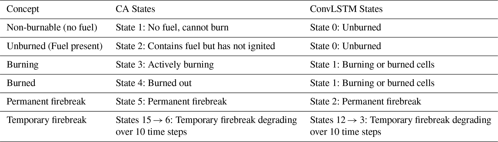
The state definitions differ slightly from those in the CA model. Using this multi-class approach, we identify both burning cells and track the duration of temporary firebreaks. The states are defined as follows:

• State 0. Unburned cells

• State 1. Burning or burned cells

• State 2. Permanent firebreaks

• States 12 → 3. Temporary firebreaks, which degrade over time and disappear after 10 time steps

The difference in state numbering between the CA simulator and the ConvLSTM model (Table 1) arises from their distinct modelling objectives. The CA simulator employs a more detailed state representation (States 1–15) to explicitly track physical fire processes and firebreak degradation. In contrast, the ConvLSTM surrogate model adopts a simplified and compact state encoding (States 0–12) to reduce the complexity of the multi-class classification task, improve training stability, and focus on the dominant fire and firebreak dynamics relevant for prediction. Temporary firebreaks in both models follow the same binary suppression logic and degrade over ten time steps; however, their numerical labels differ due to this abstraction.

Table 1 Comparison of states used in the CA simulator and the ConvLSTM surrogate model.

The model is trained using data generated by the CA model. It takes the first three time steps of fire progression, with or without firebreaks, as input and predicts the next three time steps. This 3-to-3 prediction approach is formalized in Eq. (7).

$$\begin{array}{}\text{(7)}& \left\{{\mathit{x}}_{t-\mathrm{3}},{\mathit{x}}_{t-\mathrm{2}},{\mathit{x}}_{t-\mathrm{1}}\right\}\stackrel{\text{ConvLSTMtrain}}{⟶}\left\{{\mathit{z}}_t,{\mathit{z}}_{t+\mathrm{1}},{\mathit{z}}_{t+\mathrm{2}}\right\}.\end{array}$$

The model employs the Cross Entropy loss function to evaluate training performance. In multi-class classification tasks (e.g., State 1 to 16 in this application), Cross Entropy measures the dissimilarity between the predicted probability distribution and the true class distribution, penalizing incorrect classifications more heavily. The model outputs represent the states of each cell, positioning the ConvLSTM model as performing a multi-class classification task at each pixel and time-step. The structure of our model is detailed in Table 2.

Table 2 ConvLSTM Model Summary.

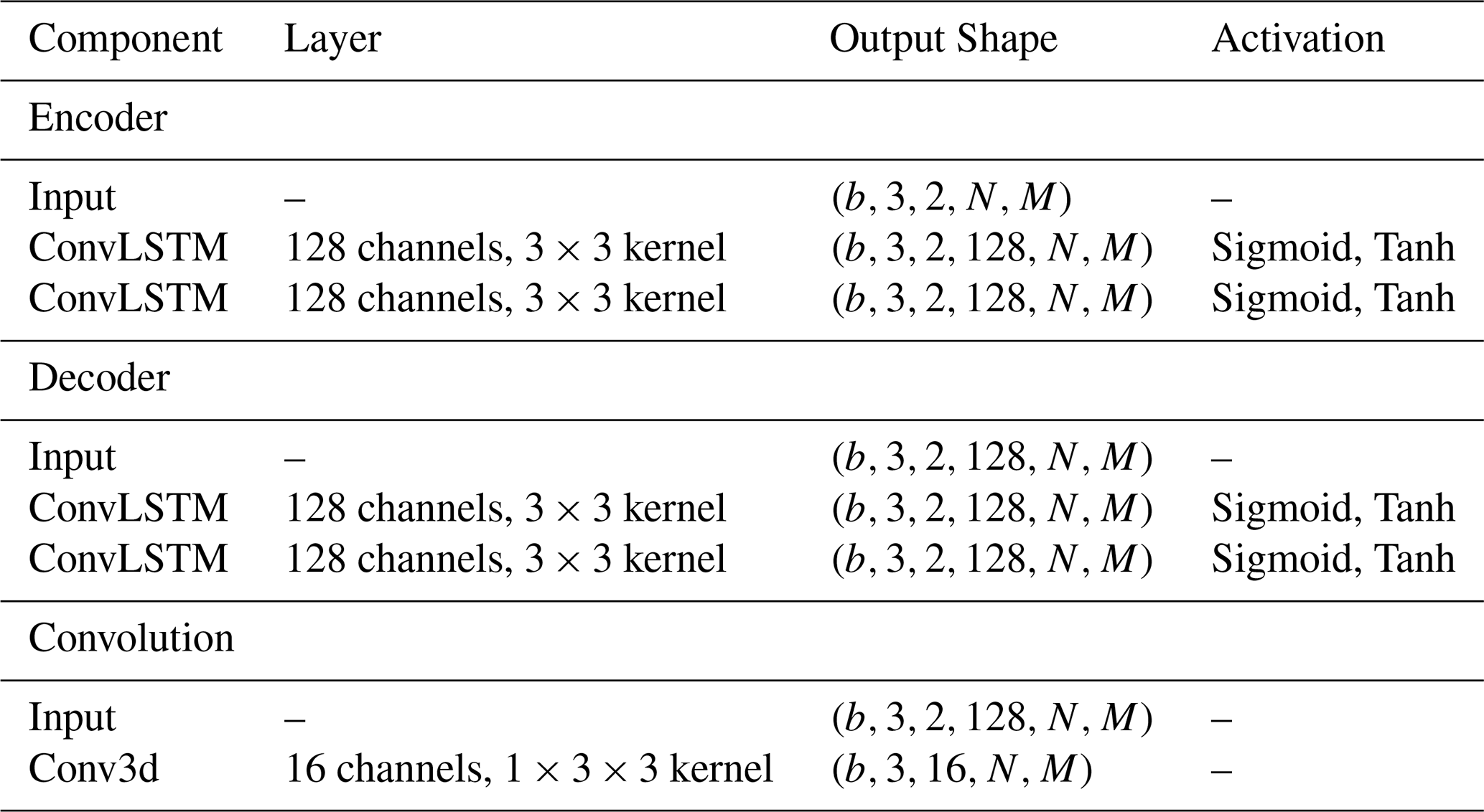
The input tensor has a shape of $(b,\mathrm{3},\mathrm{2},N,M)$, where b represents the batch size and N × M denotes the spatial dimensions of the input field. This structure indicates that we have 3 sequential frames and 2 channels. One channel encodes fire information (a matrix where 0 indicates that the pixel has not been affected by fire, 1 indicates that a pixel is either currently burning or has burned and other is for the firebreak states which is from 2 to 12). The second channel was originally designed to include landscape-related data; however, although such data are available for the selected case studies, the limited number and diversity of landscapes are insufficient to train a single generalized model that can robustly learn across different terrains. Consequently, this channel is zero-filled in the current implementation. As a result, the ConvLSTM models are trained separately for each of the three landscapes used in the CA simulations, making the current approach landscape-specific.

For the ConvLSTM layers, each unit maintains a hidden state and a current state, with 128 feature channels and a sequence length of 3. Thus, the ConvLSTM output tensor has a shape of $(b,\mathrm{3},\mathrm{2},\mathrm{128},N,M)$. After passing through the subsequent 3D convolutional layers, the final output of the model has a shape of $(b,\mathrm{3},\mathrm{16},N,M)$, where the sequence length is 3 (corresponding to 3 consecutive frames) and 16 represents the number of prediction categories (e.g., different fire spread states or fire suppression strategies).

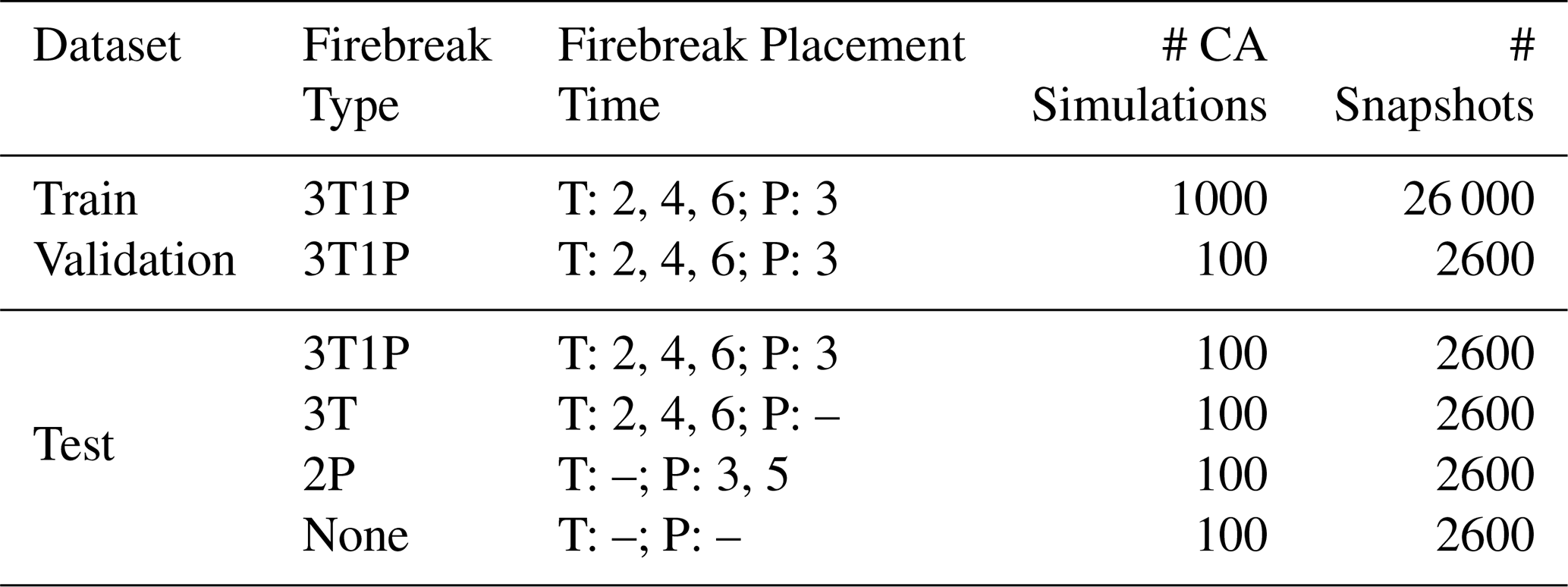
The ConvLSTM model is trained using Cross Entropy Loss on the training dataset for “Chimney 2016”, “Bear 2020”, and “Ferguson 2018” fires (Table 3) and validated on a distinct validation dataset using three metrics: Mean Squared Error (MSE), Structural Similarity Index Measure (SSIM), and Relative Prediction Error (RPE).

Table 3 Summary of dataset distribution and characteristics for training, validation, and testing for each model, categorized by landscapes: “Bear 2020”, “Chimney 2016”, and “Ferguson 2018”. The column “# CA Simulation” indicates the number of CA simulations (with different fire ignitions) that generated the datasets, with each simulation producing “# Snapshots” representing the number of CA time-steps. The model's parameters are based on each landscape's local geological characteristics, including vegetation, slope, wind speed, and other factors. “T” represents temporary firebreak placement times, and “P” represents permanent firebreak placement times. For each simulation, the ignited field is randomly selected, and the firebreak is randomly positioned around the ignited field.

The MSE measures the average squared difference between the predicted (z_t) and observed (x_t) values. This metric evaluates the overall prediction accuracy of the model, with a lower MSE value indicating better performance.

$$\begin{array}{}\text{(8)}& \text{MSE}\left({\mathit{z}}_t,{\mathit{x}}_t\right)={\displaystyle \frac{\mathrm{1}}{b}}\sum _{t=\mathrm{1}}^b\left|\right|{\mathit{x}}_t-{\mathit{z}}_t|{|}^{\mathrm{2}}\end{array}$$

The SSIM evaluates the structural similarity between the predicted and true images by considering luminance, contrast, and structural information. It ranges from −1 to 1, where a value close to 1 indicates a high degree of similarity.

$$\begin{array}{}\text{(9)}& \text{SSIM}\left({\mathit{z}}_t,{\mathit{x}}_t\right)={\displaystyle \frac{\left(\mathrm{2}{\mathit{\mu }}_{{\mathit{x}}_t}{\mathit{\mu }}_{{\mathit{z}}_t}+c_{\mathrm{1}}\right)\left(\mathrm{2}{s}_{{\mathit{x}}_t{\mathit{z}}_t}+c_{\mathrm{2}}\right)}{\left({\mathit{\mu }}_{{\mathit{x}}_t}^{\mathrm{2}}+{\mathit{\mu }}_{{\mathit{z}}_t}^{\mathrm{2}}+c_{\mathrm{1}}\right)\left(s_{{\mathit{x}}_t}^{\mathrm{2}}+s_{{\mathit{z}}_t}^{\mathrm{2}}+c_{\mathrm{2}}\right)}}\end{array}$$

The RPE is defined as the ratio of mismatched pixels between the predicted and observed fire spread landscapes, relative to the total number of pixels (N × M). This metric provides an intuitive measure of the model’s ability to correctly classify the fire spread.

$$\begin{array}{}\text{(10)}& \text{RPE}\left({\mathit{z}}_t,{\mathit{x}}_t\right)={\displaystyle \frac{\mathit{\#}\left\{{\mathit{x}}_t\ne {\mathit{z}}_t\right\}}{N\times M}}\end{array}$$

where #{x_t≠z_t} represent the number of mismatched pixels.

To assess the predictive capabilities and computational performance of our model, several wildfire datasets with different configurations were used to set up four test scenarios:

• a.

  Fire Propagation without Firebreaks: for this test scenario, a random ignition field was selected on the landscape, and fire propagation was simulated by using a CA simulator.

• b.

  Fire propagation simulation with artificial firebreaks, where artificial firebreaks were randomly placed around a randomly chosen ignition point. The cases studied include the following configurations: two permanent firebreaks (2P), three temporary firebreaks (3T), and three temporary firebreaks combined with one permanent firebreak (3T1P).

• c.

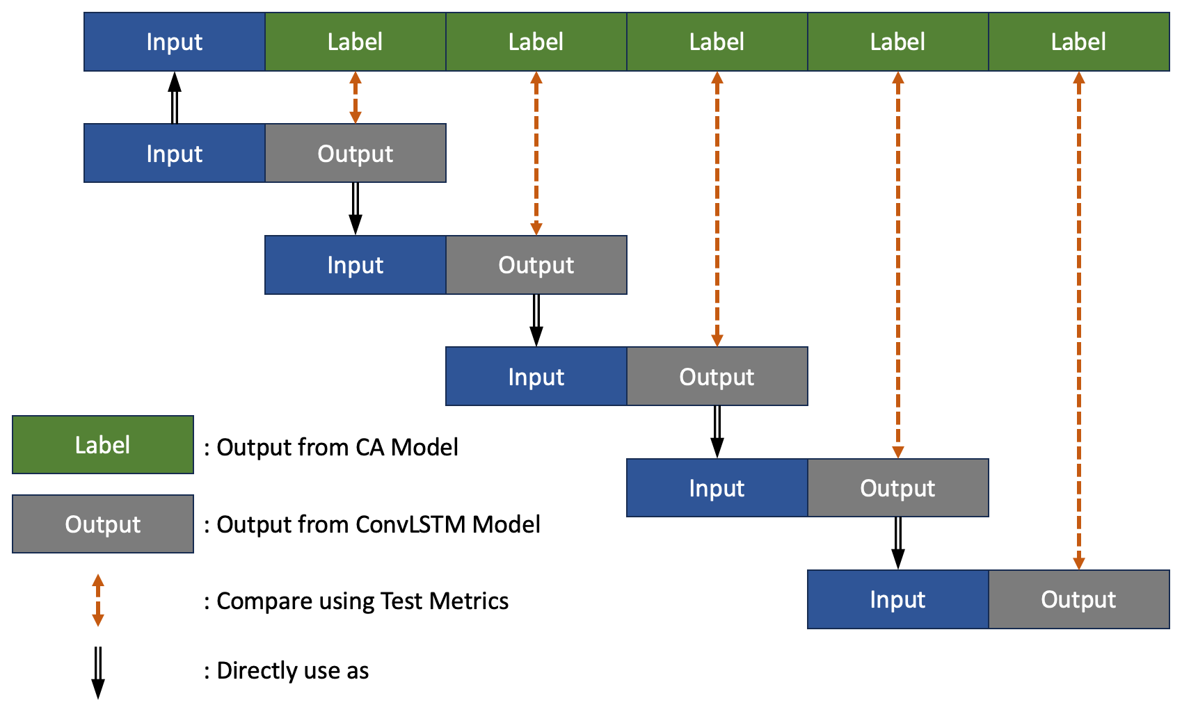
  Autoregressive fire spread predictions, to test the long-term predictive horizon and stability of the model in successive iterations. Given three time steps as initial input from the fire propagation simulation, the model generates the next three time steps. These outputs are then fed recursively back into the model as inputs for the next sequence. This process was repeated until the forecast extended to fifteen time steps beyond the initial input set (Fig. 5).

• d.

  Comparative computational efficiency. To compare the computational efficiency of our model and CA approaches, a parallel analysis of execution time and resource consumption was performed at six different spatial resolutions: 128 × 128, 256 × 256, 384 × 384, 512 × 512, 640 × 640, and 768 × 768.

Figure 5 Autoregressive fire spread predictions and compare to CA generated data.

For the three landscapes considered, each model was tested with data derived from four distinct scenarios (Table 3): (1) three temporary firebreaks combined with one permanent firebreak (3T1P), (2) three temporary firebreaks (3T), (3) two permanent firebreaks (2P), and (4) no firebreak (None). The testing data were generated using the CA simulator and matched the configurations used during model training.

To evaluate the computational efficiency of our three ConvLSTM models, we compared their efficiency with that of the CA model across varying landscape resolutions. A series of experiments was conducted using simulated wildfires, each running for 150 time steps on landscapes of increasing size (from 128 × 128 to 768 × 768). For each landscape resolution, the runtime to predict three consecutive time steps – corresponding to a single ConvLSTM inference – was recorded. To ensure stability and consistency in the results, the average runtime was computed over the full 150-step simulation period. The goal was to evaluate the models' speed and their ability to handle large-scale landscapes, which is essential for real-world wildfire datasets that require high-resolution simulations to capture intricate spatial details.

3 Results

3.1 Model Performance

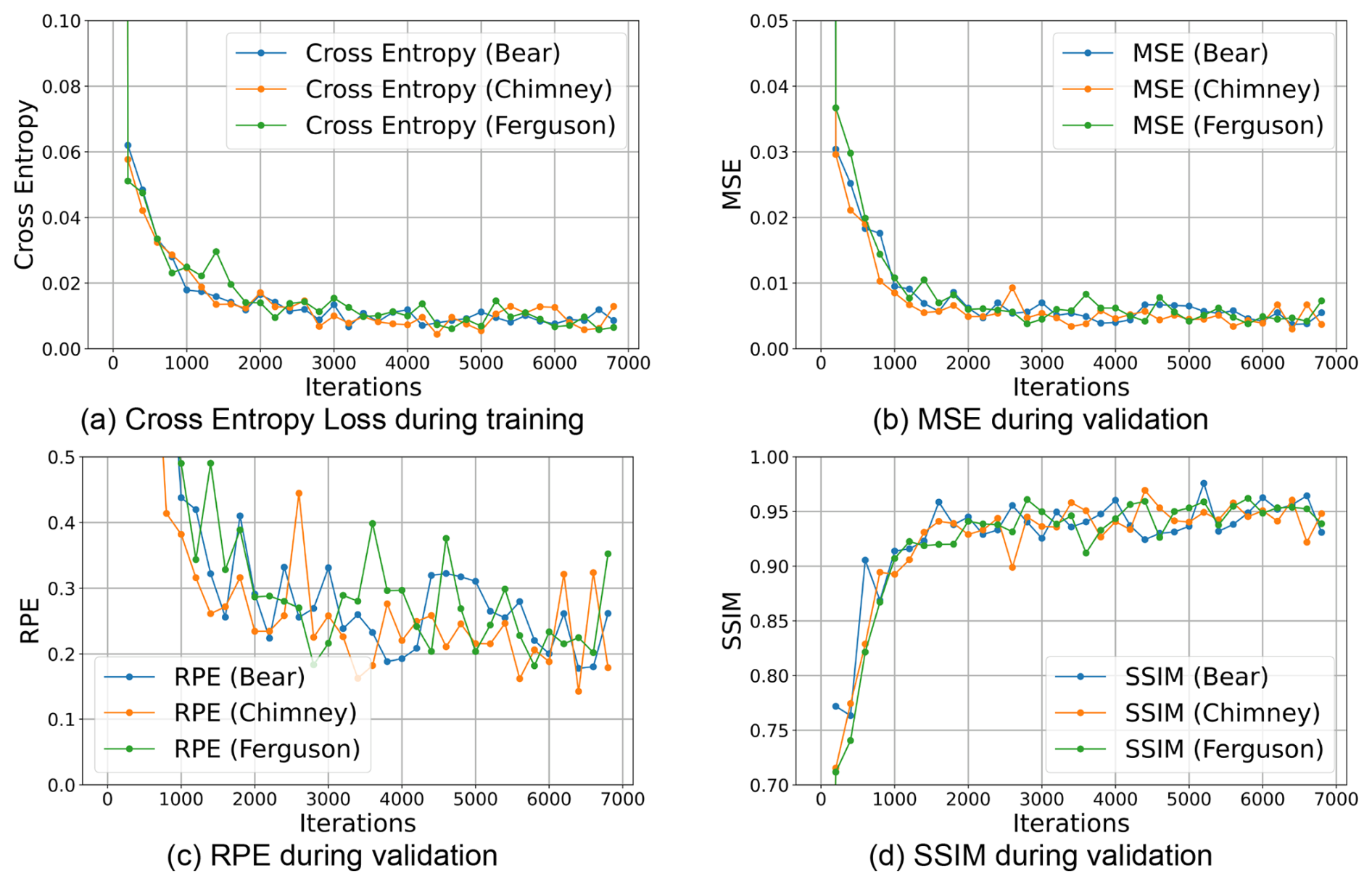
Analysis of the Chimney 2016, Ferguson 2018 and Bear 2020 simulations show that all metrics converge to acceptable levels: the Cross Entropy Loss during training phases (Fig. 6a), remains below 0.02, the MSE (Fig. 6b), remains below 0.01, RPE (Fig. 6c) stabilizes around 25 % and SSIM for the validation phase (Fig. 6d) is consistently higher than 0.9. These results show that the model is not only learning effectively but is also achieving strong performance on unseen data. The consistent validation metrics suggest that the model generalizes well and is robust against over-fitting.

Figure 6 Metric values during the training process.

All models demonstrated comparable performance across different configurations (Fig. 7). Scenarios with firebreaks (3T1P, 3T and 2P) had higher prediction accuracy than those without (None). This improved performance can be attributed to the controlled conditions provided by firebreaks, which limit fire spread, reduce system randomness, and enhance prediction reliability. The absence of constraints on fire spread in the scenarios with no firebreaks introduces greater randomness in the CA simulation. The two-permanent-firebreak (2P) scenario had higher uncertainty than the other firebreak scenarios because the 90 % suppression rate introduced additional stochastic factors. Although both the no firebreak (None) and the two permanent firebreaks (2P) scenarios had poorer performance and higher standard deviations, nevertheless the results remain within acceptable limits.

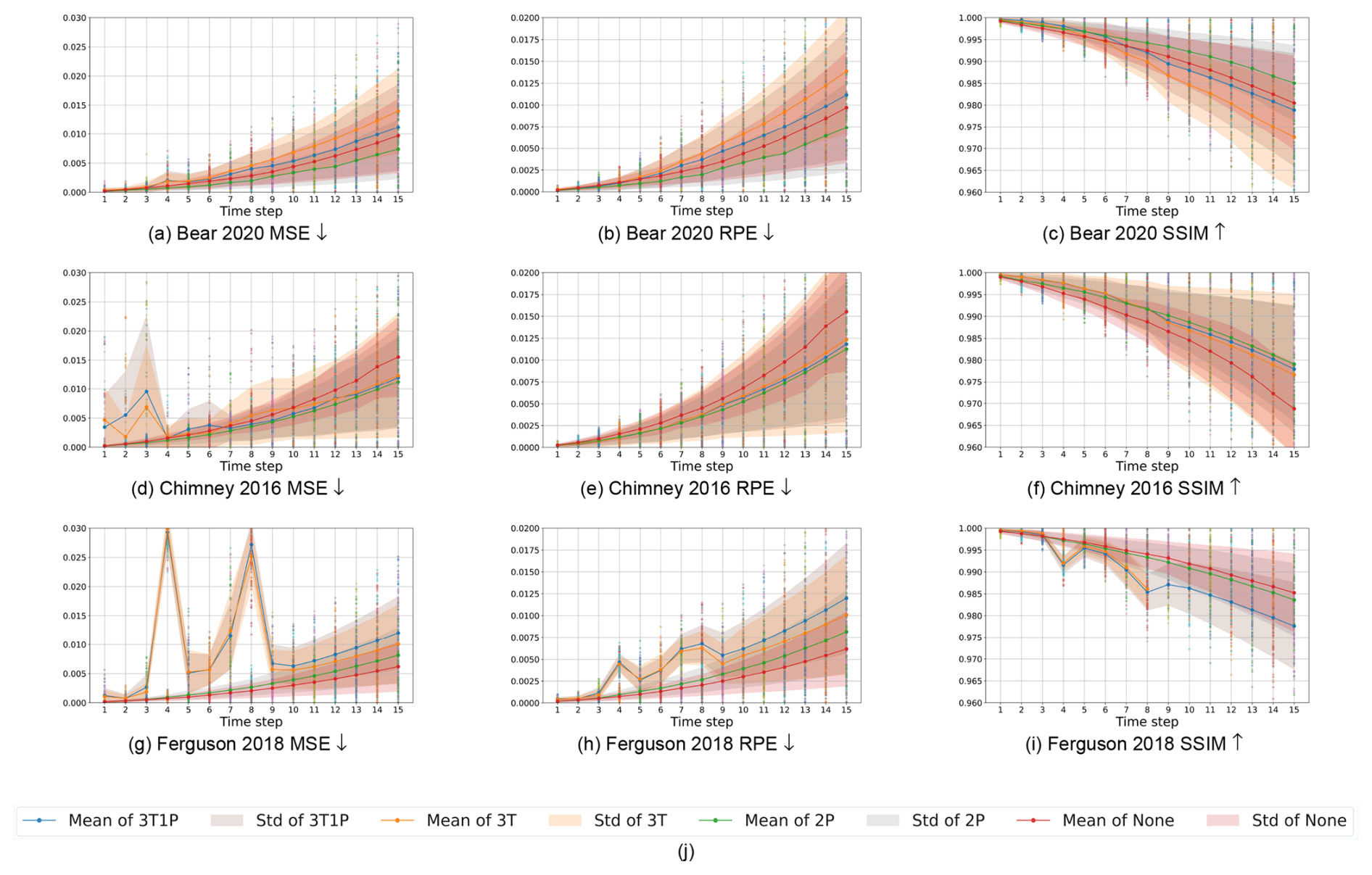
Figure 7 Testing models on metric MSE, RPE and SSIM with different configurations. The solid line is the mean of the data after filter outliers and the shadow represent the standard deviation.

Although iterative testing inevitably results in error accumulation over time, the models retained strong predictive accuracy even after multiple iterations. The average MSE was below 0.01 for the first three time steps, and remained under 0.03 across the entire 15-step sequence (Fig. 7a, d, g). The mean RPE was under 0.75 % for the first nine time steps, and stayed below 1.5 % for the full sequence (Fig. 7b, e, h). The mean SSIM value exceeded 0.99 for the first six time steps and remained above 0.97 throughout the entire sequence (Fig. 7c, f, i), indicating strong structural similarity between the predicted and actual fire spread.

In Fig. 7, the improved predictive accuracy observed in scenarios with firebreaks can be attributed to the reduced stochasticity and constrained fire spread dynamics introduced by suppression measures. Firebreaks limit the spatial extent and rate of fire propagation, thereby reducing the number of possible spread pathways and dampening the inherent randomness of the CA simulations. This constraint leads to more structured and predictable fire evolution patterns, which are easier for the ConvLSTM model to learn and generalize. In contrast, scenarios without firebreaks exhibit more unconstrained fire growth and higher variability, increasing the difficulty of accurately predicting long-term spread. As a result, the presence of firebreaks not only mitigates fire propagation in the simulations but also enhances the stability and learnability of the underlying spatio-temporal patterns captured by the model.

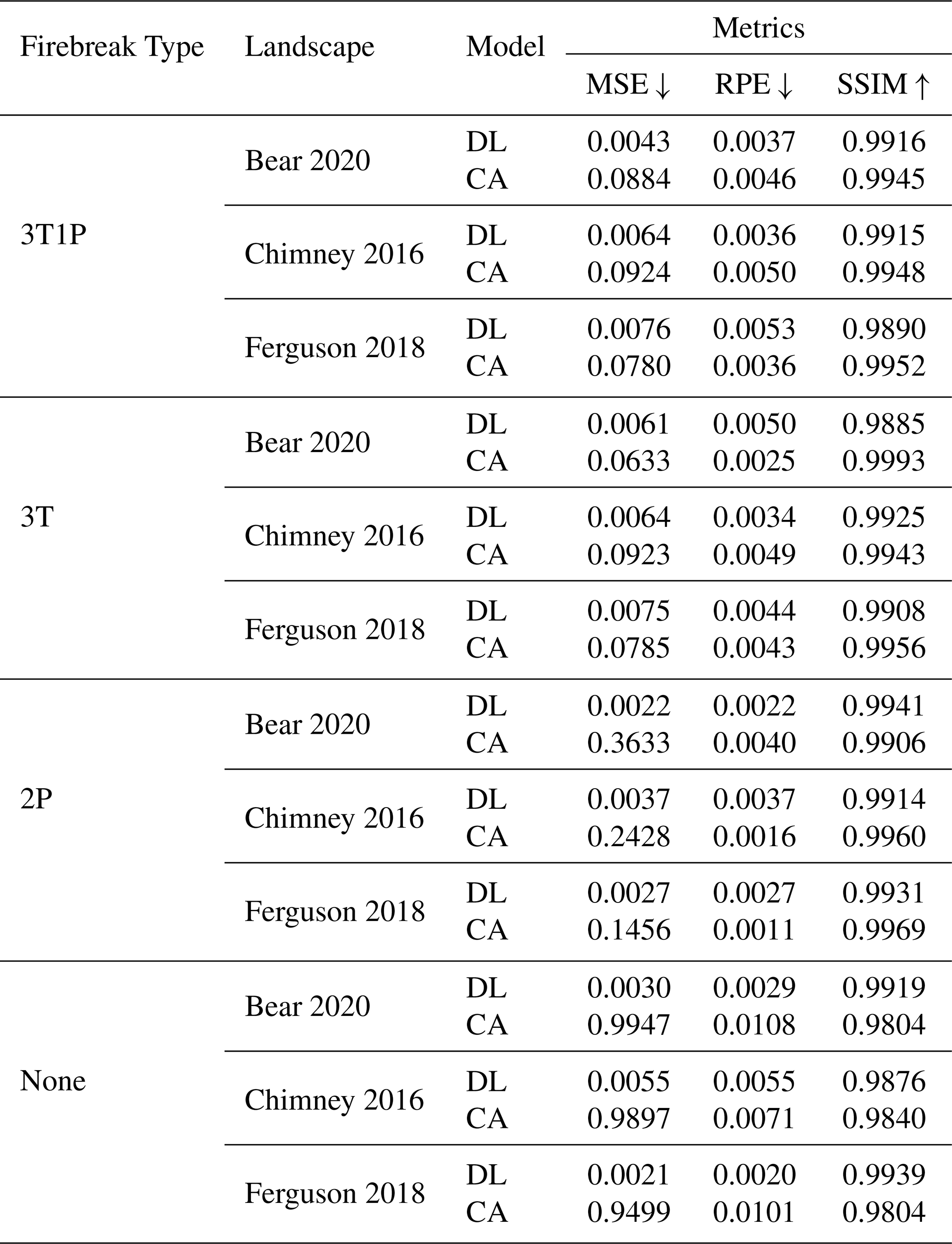
Although there is an inherent challenge of cumulative errors in iterative modelling, the error maps (Fig. 8, C2, C3, C4, C5, C6, C7, C8) show only small deviations between the predicted and target values even after five loops. Thus, the models effectively maintain accuracy under iterative testing conditions and have successfully learned the dynamics associated with both temporary and permanent firebreaks. Specifically, the models recognize that temporary firebreaks disappear after ten time steps, achieving a suppression rate nearing 100 % while permanent firebreaks do not disappear but have a lower suppression rate. The CA model provides comparable accuracy to the DL model (Table 4). However, the DL model is significantly faster.

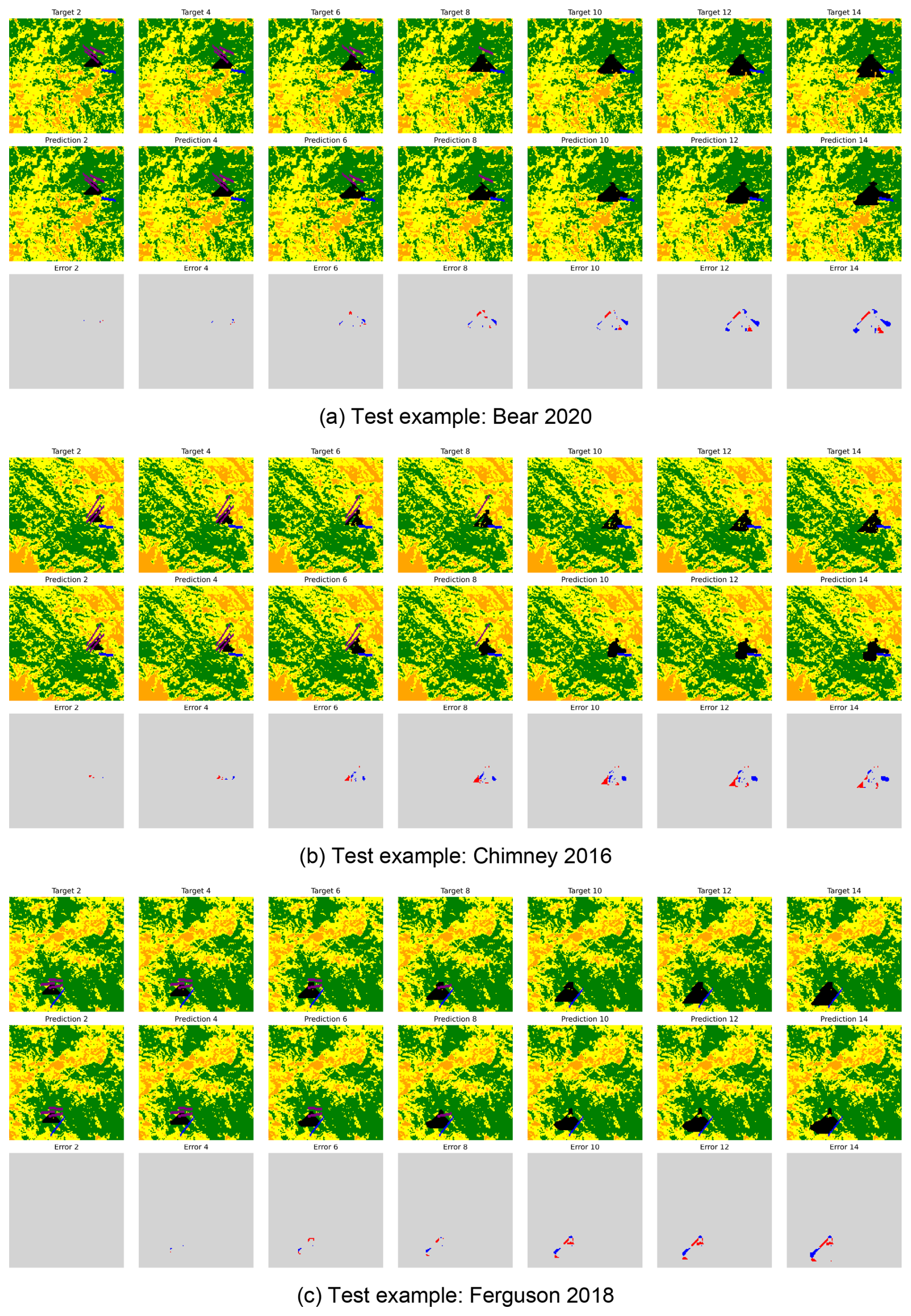
Figure 8 Here we tested each landscape using an autoregressive testing approach, performing 5 iterative loops that will generate the following 15 time-steps and we plot the result for every 2 time-steps. For the error map, red means false negatives and blue means false positive. A cropped and zoomed-in version is provided in Appendix C (Fig. C2), where the background is neutralized to emphasize the active fire scene and associated fire spread patterns.

Table 4 Comparison of Metrics Across Different Fire Suppression Strategies, Landscapes, and Models. For the DL model, the values represent the mean of the metric of the middle three time-steps' (sixth, seventh, eighth) tested on 100 CA simulations each has 26 CA time-steps (Table 3). For the CA model, the values represent the mean metric calculated over three time steps, using the same initial conditions across four separate simulations.

The magnitude and spatial distribution of false positives and false negatives differ among the three wildfire cases, reflecting intrinsic differences in fire behaviour across landscapes. The Ferguson 2018 case exhibits relatively smaller error regions, whereas the Chimney 2016 and Bear 2020 cases show more pronounced deviations. This variation is likely associated with differences in vegetation density, fuel continuity, and wind-driven spread intensity across the study areas. Fires that propagate more rapidly or exhibit stronger directional bias due to wind forcing generate more complex and rapidly evolving fire fronts, which amplify autoregressive prediction errors over successive iterations. In contrast, slower or more spatially constrained fires produce more structured propagation patterns that are easier for the surrogate model to approximate.

In addition, because the ConvLSTM model does not explicitly incorporate detailed topographic features or spatially variable wind fields as dynamic inputs, the model must implicitly learn these effects from the CA-generated training data. This limitation may contribute to the larger discrepancies observed in landscapes where fire spread is more sensitive to environmental heterogeneity. Future work could integrate higher-resolution environmental forcing and real-time satellite observations through data assimilation strategies to dynamically correct prediction drift and improve long-term stability.

While the results demonstrate strong predictive capability within the tested configurations, it is important to recognize the methodological limitations of the current framework. Wind speed, wind direction, and slope effects are incorporated within the CA simulations to generate the training data. However, wind forcing was assumed to be spatially constant within each simulation, and detailed topographic information was not explicitly provided as dynamic input channels to the ConvLSTM model. In real wildfire events, spatially heterogeneous wind fields, gust dynamics, and terrain-induced flow effects can substantially alter fire spread behaviour. These simplifications reduce the dimensionality of the training space and allow controlled evaluation of the surrogate modelling approach, but they also limit direct operational realism. Future studies should incorporate higher-resolution meteorological inputs and explicit topographic features as model inputs to better represent complex fire–environment interactions.

3.2 Inference Speed Evaluation

The ConvLSTM model, executed on an NVIDIA A100 PCIE GPU, completed simulations of 3 time steps for all resolutions from 128 × 128 to 768 × 768 in under 0.2 s (Fig. 9). The ConvLSTM's computation time increased linearly with landscape size, whereas the CA model, executed on a CPU, showed significantly higher computational costs overall and computation time increased exponentially with larger landscape sizes. For the maximum resolution of 768 × 768, the CA model required nearly 50 s to predict three time steps, approximately 250 times longer than the ConvLSTM model. The faster speed of the ConvLSTM models arises partly from the efficiency of the model architecture but also from the advantages of GPU acceleration. The reported 250 times speed-up corresponds to a comparison between a GPU-accelerated ConvLSTM model and a CPU-based CA implementation, reflecting realistic deployment conditions. When executed on CPU, the ConvLSTM model is computationally more demanding than CA, as expected for convolutional neural networks without hardware acceleration.

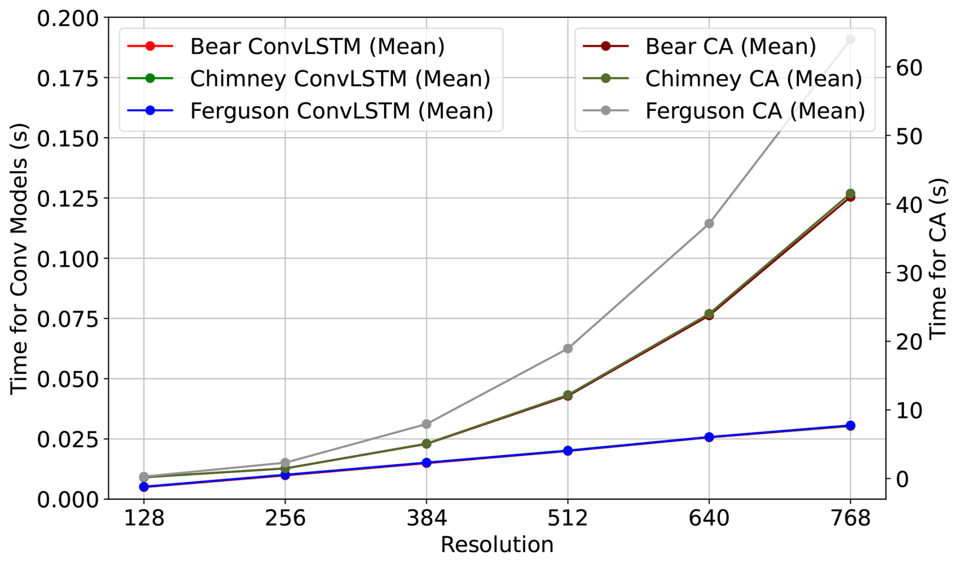
Figure 9 Prediction time (in seconds) for completing 3 steps of simulation across various landscape resolutions (128 × 128 to 768 × 768). The CA Model using CPU and the ConvLSTM Model using NVIDIA A100 PCIE GPU.

4 Conclusion and Future directions

The ConvLSTM model has good performance in simulating wildfire propagation combined with firebreak deployment. It accurately identifies different types of firebreaks, evaluates their efficiency, and predicts how long they last. In comparison with the CA model, which is simple and highly interpretable but has a high computation cost, the speed of ConvLSTM model across varying input sizes makes it useful for real-world, real-time applications.

Wildfire propagation is inherently stochastic, and the autoregressive approach amplifies prediction errors over time. The task becomes more difficult in high-altitude regions where burning is less likely, especially since explicit landscape features are not provided as model inputs. The absence of key drivers like wind speed and direction further limits predictive accuracy. Despite these challenges, the model demonstrates consistent predictive capability within the tested scenarios and successfully captures key fire–firebreak interactions.

It is important to emphasize that the present work represents a methodological proof of concept rather than a fully operational wildfire forecasting system. The primary objective was to demonstrate that a ConvLSTM-based surrogate model can learn wildfire spread dynamics in the presence of dynamic firebreak deployment under controlled simulation settings. To maintain tractability of the training space, wind forcing was assumed to be spatially constant within each simulation, and landscape information was simplified. While these assumptions limit direct operational applicability, they allow for controlled evaluation of the surrogate modelling framework. Future work will focus on incorporating spatially and temporally variable wind fields, gust dynamics, detailed topographic information, and additional fuel characteristics into the training datasets. By enriching the diversity of environmental forcing scenarios, the model can learn greater sensitivity to key drivers of wildfire behaviour, thereby improving realism and extending its applicability to operational contexts. The model could be further improved by using detailed landscape data, including vegetation types, densities, moisture levels, and topographical features, as model inputs. This would allow the development of a universal model that performs well across various geographic regions, minimizing the need to tune the model for each fire event. Incorporating dynamic meteorological information and wind patterns would also enhance prediction accuracy. Future work will also consider generative AI methods for stochastic fire spread prediction (Yu et al., 2026; Cheng et al., 2023) to enhance uncertainty quantification.

More realistic characterisation of firebreak placement and experiments to optimise placement under realistic conditions would also enhance the usefulness of the model and contribute to more context-aware forecasting, benefiting wildfire management and containment strategies.

Appendix A: Main Notations

Notation	Description
Cellular Automata Simulator
Pburn	Probability that a cell that can be burned but not ignited (State 2) ignites if a neighbouring cell is burning.
Rburned_down	Probability that a burning cell (State 3) transitions to a burned-down state (State 4).
Rpfb	Suppression rate for cells in a permanent firebreak (State 5).
Ppfb_burn	Probability that a cell in a permanent firebreak burns, calculated as (1−Rpfb)Pburn.
ph	Base burning probability.
pveg	Factor accounting for local vegetation density.
pden	Factor accounting for canopy cover.
ps	Slope effect on fire spread, modelled as ps=exp (aθs).
θs	Slope angle between adjacent or diagonal cells.
E1, E2	Elevations of the respective cells (adjacent or diagonal), used in slope angle calculation.
l	Cell length used in slope angle calculation.
pw	Wind effect on fire spread, modelled as pw=exp (c1Vw)exp (Vwc2(cos (θw)−1)).
Vw	Wind speed in meters per second.
θw	Angle between wind direction and potential fire spread direction.
c1, c2	Tunable coefficients for wind effect.
ConvLSTM Model
fConvLSTM	The ConvLSTM predictive model.
W(⋅)	Learnable weight matrix of filter parameters.
σ	Sigmoid activation function.
ft, it, ot	Activations of the LSTM forget, input, and output gates, respectively.
${\stackrel{\mathrm{̃}}{\mathit{C}}}_t$	Candidate cell state value at time t.
Ct	Actual cell state at time t.
N × M	Dimensions of the field being processed, where N is the number of rows and M is the number of columns.
b	Batch size for model training and prediction.
S	Set of possible pixel states or classes.
xt	Burnt area at time t of dimension N × M, generated by the CA simulator.
zt	Model output at time t, representing a hidden state feature matrix that predicts the next frame of wildfire progression in an N × M grid format.
bi, bf, bo, bs	Bias vectors associated with the input, forget, output gates, and cell state candidate, respectively.

Appendix B: Acronyms

ML	Machine Learning
RNN	Recurrent Neural Network
LSTM	Long Short-Term Memory
DL	Deep Learning
ConvLSTM	Convolutional Long Short-Term Memory
CA	Cellular Automata
DEVS	Discrete Event System Specification
MODIS	Moderate Resolution Imaging Spectroradiometer
VIIRS	Visible Infrared Imaging Radiometer Suite
IFTDSS	Interagency Fuel Treatment Decision Support System
MSE	Mean Squared Error
SSIM	Structural Similarity Index Measure
RPE	Relative Prediction Error

Appendix C: More test example

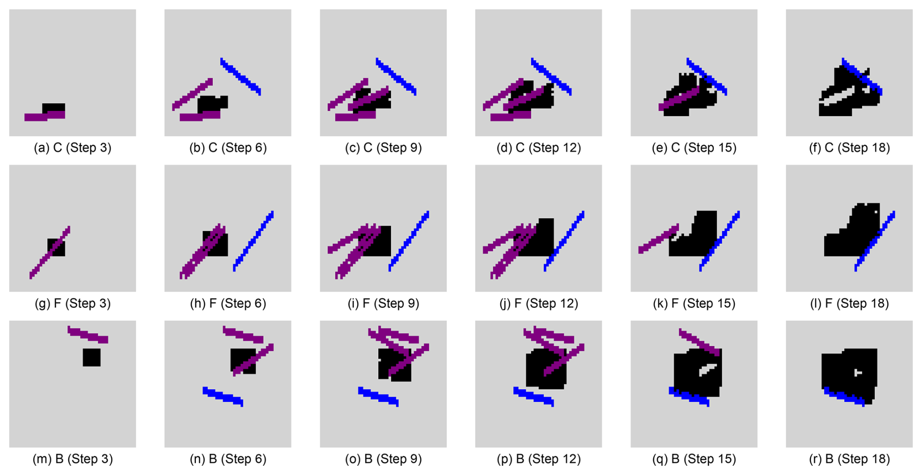
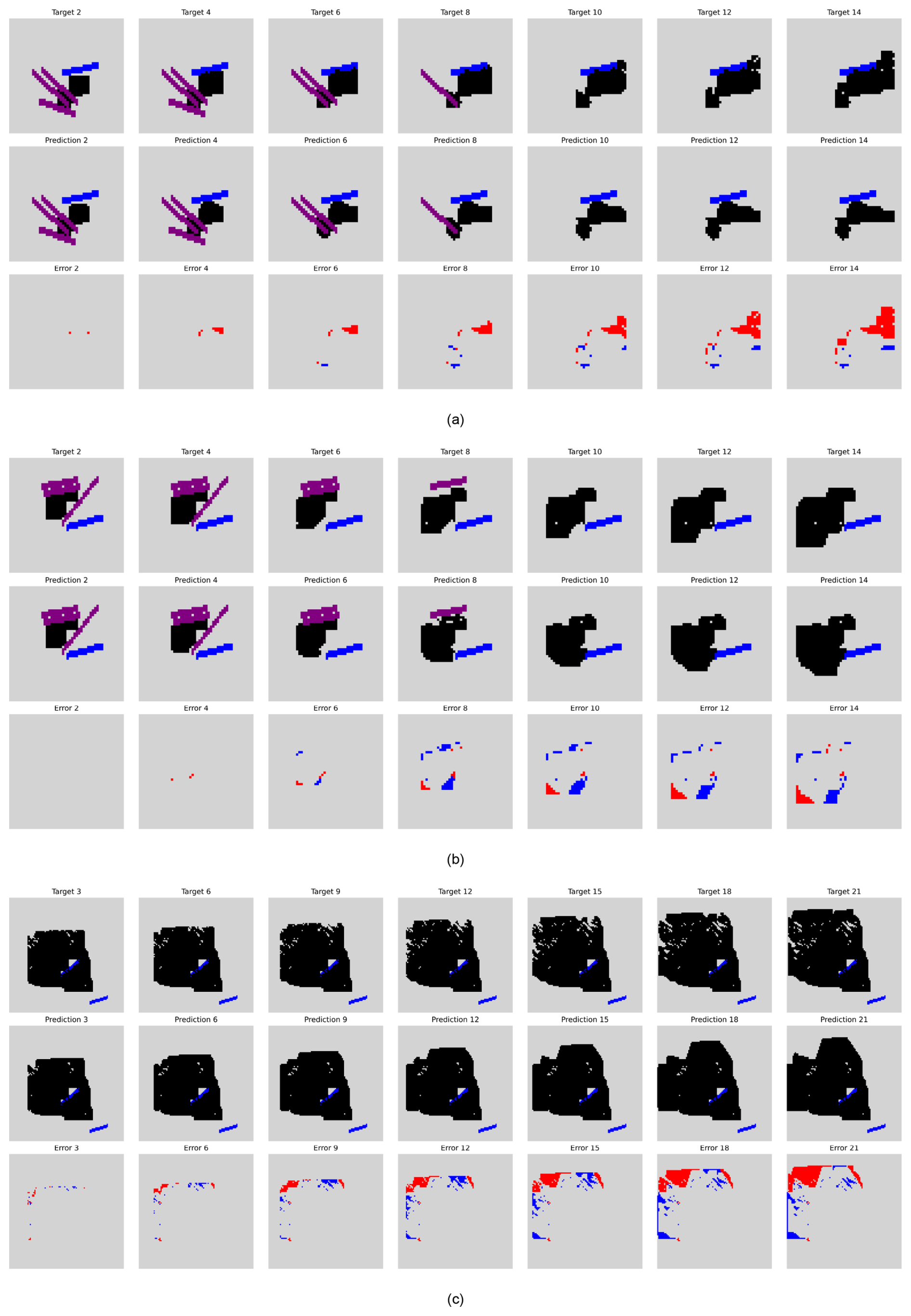
Figure C1 Cropped and zoomed-in view of Fig. 4, with the background neutralized to highlight the active fire scene and fire spread dynamics.

Figure C2 Cropped and zoomed-in view of Fig. 8, with the background neutralized to highlight the active fire scene and fire spread dynamics.

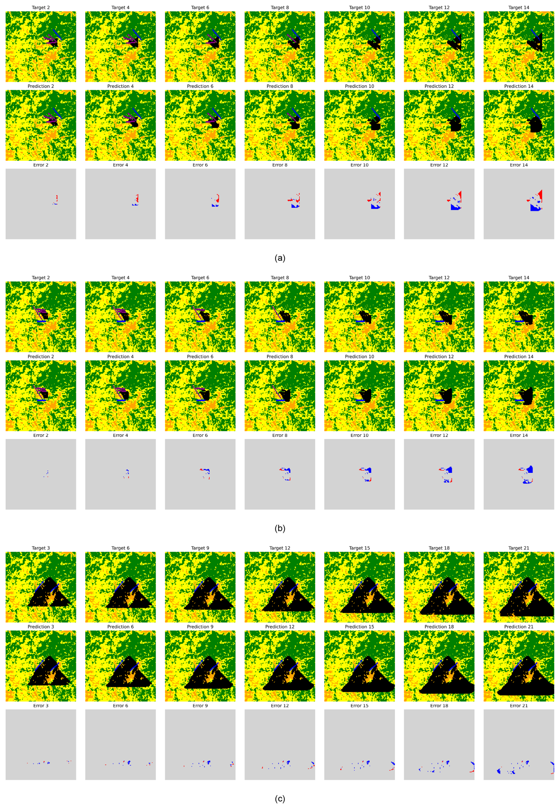
Figure C3 Bear 2020 test example. In panels (a) and (b), we performed 5 iterative loops, generating 15 time-steps, with the results plotted every 2 time-steps. In contrast, in panel (c), we conducted 7 iterative loops, generating 21 time-steps, and plotted the results every 3 time-steps. For the error image, red indicates false negatives, while blue represents false positives.

Figure C4 Cropped and zoomed-in view of Fig. C3, with the background neutralized to highlight the active fire scene and fire spread dynamics.

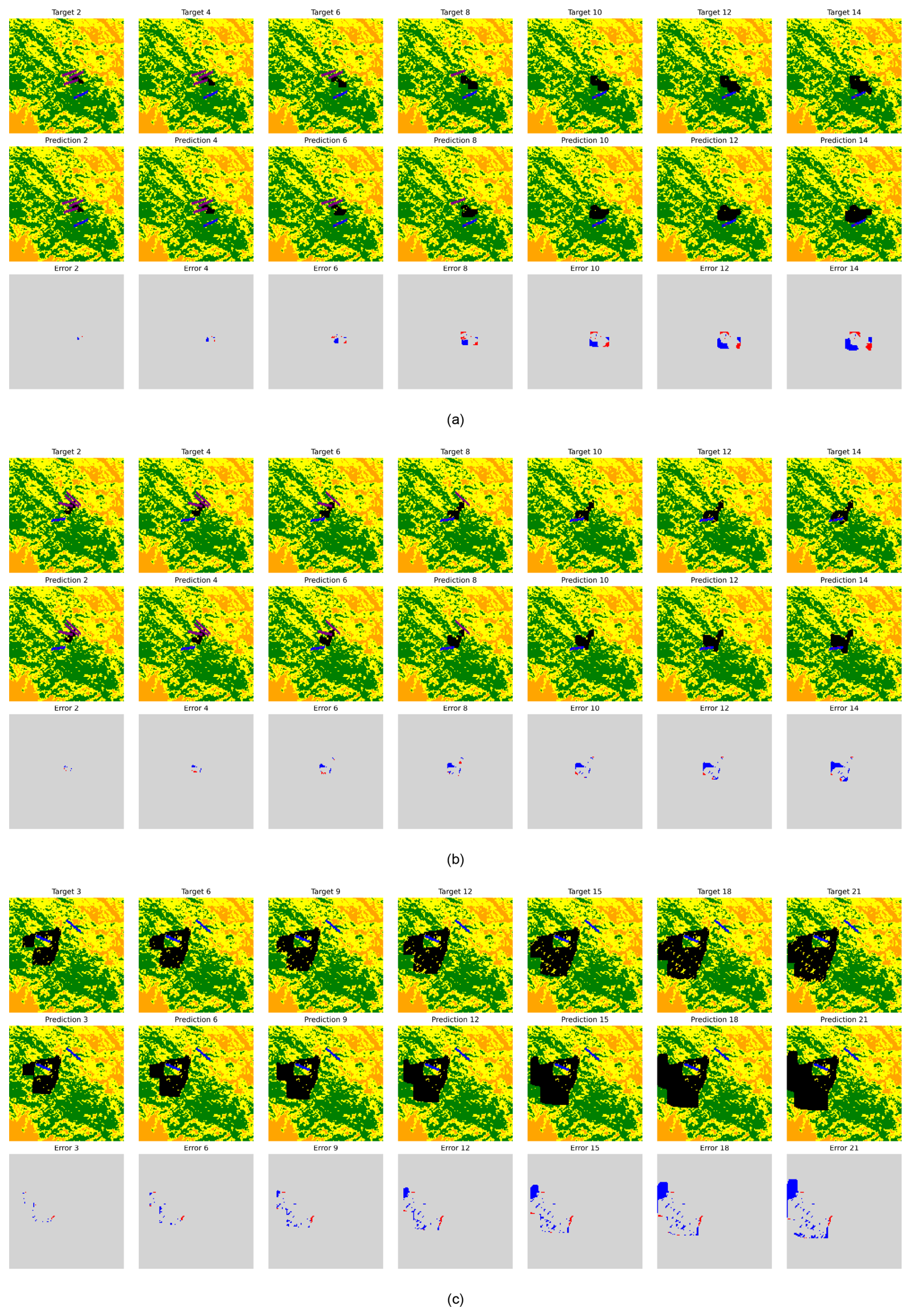
Figure C5 Chimney 2016 test example. In panels (a) and (b), we performed 5 iterative loops, generating 15 time-steps, with the results plotted every 2 time-steps. In contrast, in panel (c), we conducted 7 iterative loops, generating 21 time-steps, and plotted the results every 3 time-steps. For the error image, red indicates false negatives, while blue represents false positives.

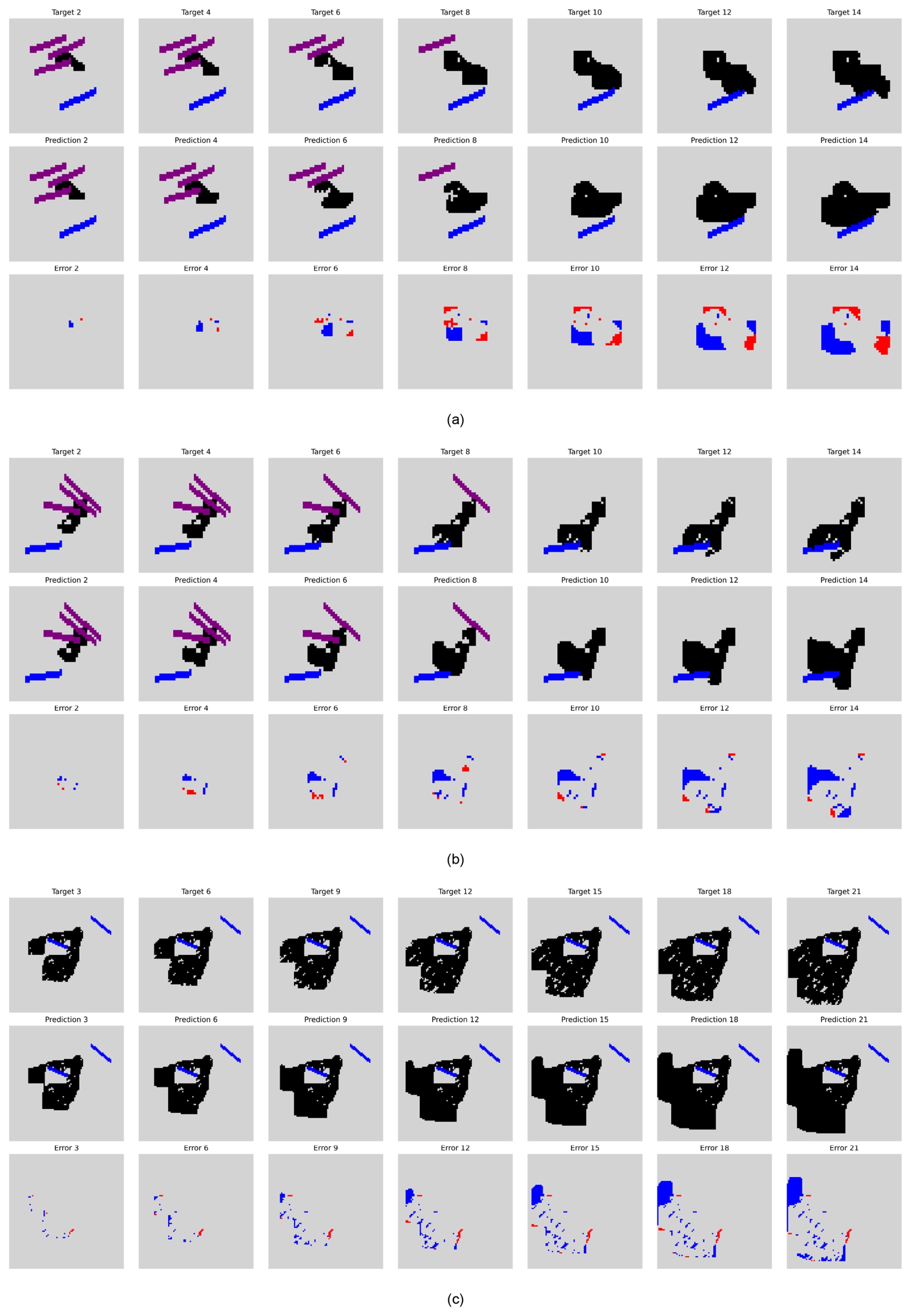
Figure C6 Cropped and zoomed-in view of Fig. C5, with the background neutralized to highlight the active fire scene and fire spread dynamics.

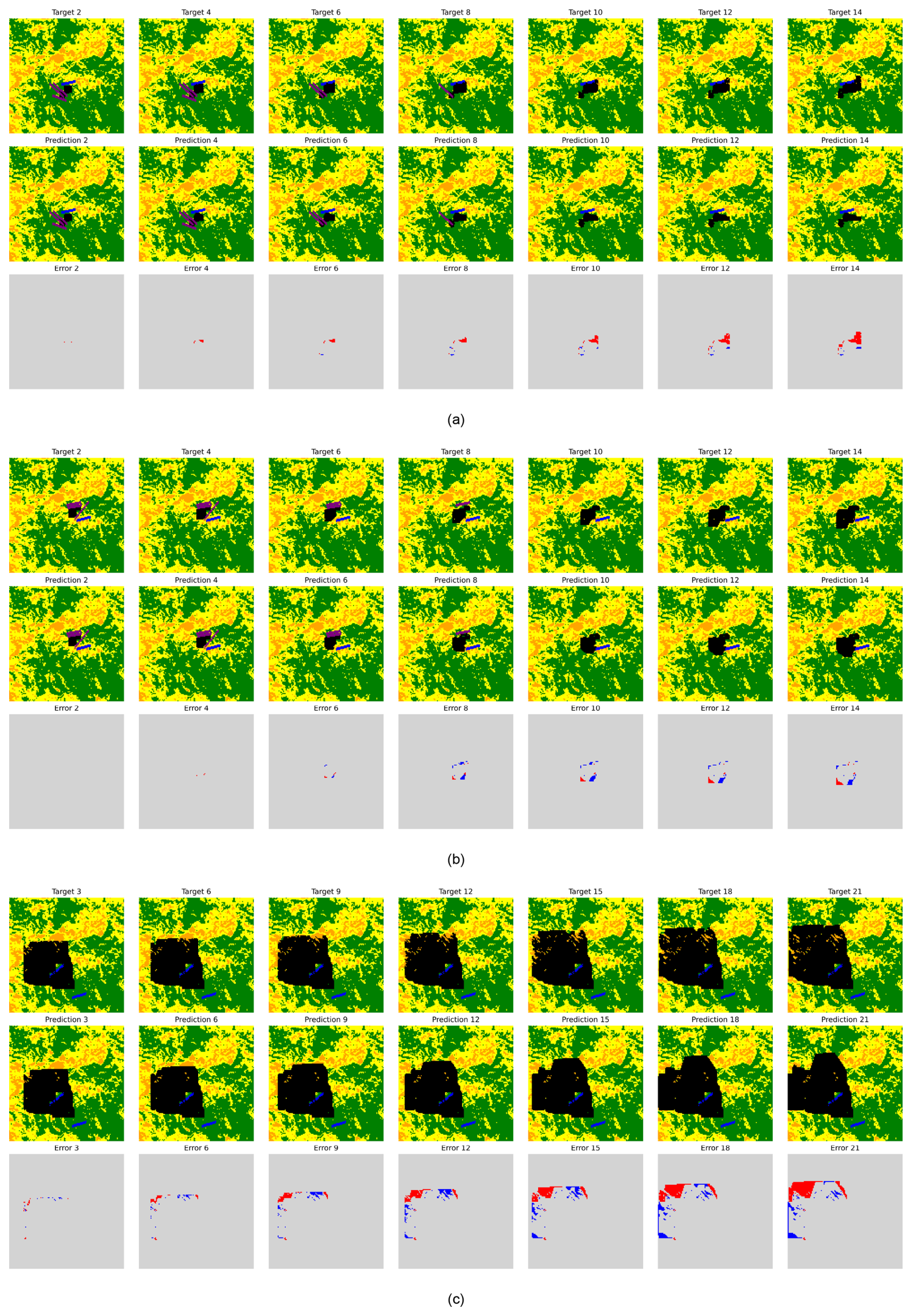
Figure C7 Ferguson 2018 test example. In panels (a) and (b), we performed 5 iterative loops, generating 15 time-steps, with the results plotted every 2 time-steps. In contrast, in panel (c), we conducted 7 iterative loops, generating 21 time-steps, and plotted the results every 3 time-steps. For the error image, red indicates false negatives, while blue represents false positives.

Figure C8 Cropped and zoomed-in view of Fig. C7, with the background neutralized to highlight the active fire scene and fire spread dynamics.