Evaluation of microphysics and boundary layer schemes for simulating extreme rainfall events over Saudi Arabia using WRF-ARW

Extreme Rainfall Events (EREs) and resulting flash floods in Saudi Arabia pose major threats, frequently causing fatalities and significant economic losses. Accurate ERE simulations are crucial for weather forecasting, climate change assessment, and disaster management. This study evaluates planetary boundary layer (PBL) and cloud microphysics (MP) schemes to simulate EREs in the Arabian Peninsula (AP) using the Advanced Research version of the Weather Research and Forecasting (WRF-ARW) model V4.4. Thirty-six combinations of four PBL and nine MP schemes were tested across 17 EREs at a convection-permitting 3 km resolution and compared with IMERG gridded satellite data for rainfall and station observations for temperature, humidity, and wind speed. The Kling–Gupta Efficiency (KGE), which incorporates correlation, variability, and bias, was used as performance metric. We found a good agreement between observed and simulated rainfall patterns, though some over- and underestimations were present. Among the PBL schemes, Yonsei University (YSU; BL1) tended to perform best in terms of rainfall, while Thompson (MP8) ranked the highest among the MP schemes. Goddard (MP7) also delivered strong results. Among all 36 combinations, the Thompson-YSU (MP8_BL1) combination produced the highest mean KGE across the 17 EREs for rainfall, performing statistically significantly better than 21 other combinations. While MP8_BL1 also performed best for the other three meteorological variables, performance rankings varied across variables, likely because different physical processes govern the simulation of different variables. This study highlights the complexity of scheme evaluation and the importance of analyzing multiple EREs with high-quality reference data. The results offer practical guidance for scheme selection and lay the foundation for improving ERE forecasting and regional climate modeling over the AP.

1 Introduction

Extreme Rainfall Events (EREs) are episodes of intense rainfall over a short duration, often resulting in flash floods, landslides, severe damage to infrastructure and property, and loss of life (Easterling et al., 2000; Houze, 2012; Kundzewicz et al., 2014). These events are becoming more frequent and intense as atmospheric moisture increases by about 7 % per degree of warming, following Clausius–Clapeyron scaling (e.g., Held and Soden, 2006; O'Gorman and Schneider, 2009; Muller and Takayabu, 2020; Fowler et al., 2021). Although mean rainfall increases at a slower rate of 2 %–3 % per degree, EREs can intensify by as much as 6 %–10 % depending on their spatial and temporal scales (e.g., Allan and Soden, 2008; O'Gorman and Schneider, 2009), significantly increasing their potential for destructive impacts.

Despite its arid desert climate and low annual rainfall, Saudi Arabia regularly experiences significant EREs (Almazroui, 2011; Haggag and El-Badry, 2013; Deng et al., 2015; Yesubabu et al., 2016; Atif et al., 2020), particularly during the rainy season from November to April. These events are frequently associated with intrusions of an intensified subtropical jet stream, mid-latitude cyclonic disturbances, and the low-level advection of warm, moist air from nearby water bodies, including the Red Sea, Arabian Gulf, and Arabian Sea (Evans et al., 2004; Barth and Steinkohl, 2004; Evans and Smith, 2006; De Vries et al., 2013, 2016). Though infrequent, these EREs cause substantial damage (Al Saud, 2010; Youssef et al., 2016), making accurate forecasting and projection essential for disaster management, early warning systems, and climate adaptation in the region (Hijji et al., 2013; Abosuliman et al., 2014).

Advanced Research version of the Weather Research and Forecasting (WRF-ARW; Skamarock et al., 2019) is a widely used Numerical Weather Prediction (NWP) model in the Arabian Peninsula (AP) to simulate and forecast EREs (Deng et al., 2015; Taraphdar et al., 2021; Luong et al., 2025; Francis et al., 2025). These models are subject to various sources of uncertainty, particularly due to parameterizations. Two key parameterization schemes that strongly influence ERE simulations include the Planetary Boundary Layer (PBL) and cloud microphysics (MP) schemes.

The PBL scheme governs the vertical exchange of momentum, heat, and moisture between the surface and the atmosphere, playing a critical role in simulating near-surface conditions. It regulates vertical mixing and turbulence, which are essential for atmospheric instability and convective initiation – key processes that directly impact rainfall development (Kumar et al., 2008). The selection of an appropriate PBL scheme is especially important in arid and semi-arid regions such as the AP, as intense surface heating in desert environments leads to the formation of unusually deep PBLs, sometimes extending up to 5 km during the day (Gamo, 1996; Marsham et al., 2008; Ntoumos et al., 2023). This necessitates the use of a scheme capable of accurately modeling the vertical distribution of heat, moisture, and momentum within such a deep layer. Furthermore, deserts are characterized by complex thermodynamic profiles, including sharp temperature gradients and significant humidity variations, which complicate the modeling process. Strong diurnal temperature variations also require a PBL scheme capable of effectively capturing short-term fluctuations in energy and moisture fluxes.

The MP scheme governs the evolution of cloud particles, including cloud droplets, rain, snow, and ice, which are essential to determine the intensity and duration of rainfall (Dudhia, 2014). It controls cloud formation, rainfall processes, and interactions between different water phases. It also influences radiative transfer by affecting cloud optical properties such as droplet size distribution, phase, and concentration (Stull, 1988; Garratt, 1994; Dudhia, 2014). Additionally, MP schemes govern key hydrometeor processes like condensation and coalescence, which directly impact the timing, intensity, and spatial distribution of rainfall. Both single-moment and double-moment schemes exist; the latter provide a more detailed representation by also predicting number concentrations of hydrometeors (see, e.g., Kessler, 1969; Chen and Sun, 2002; Hong et al., 2004; Rogers et al., 2001; Hong and Lim, 2006; Tao et al., 2016; Thompson et al., 2008; Morrison et al., 2009).

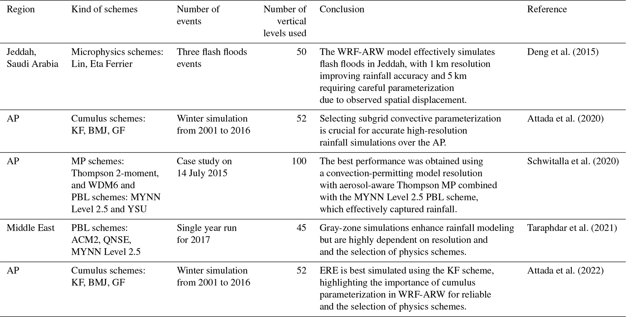
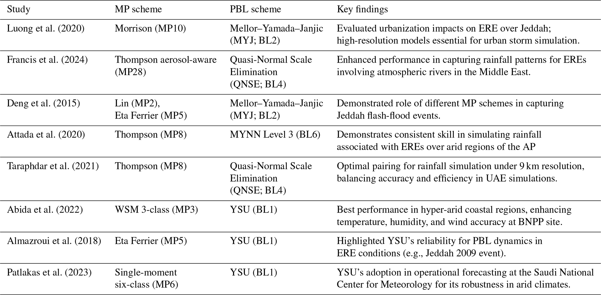
Although several previous studies have evaluated different WRF-ARW parameterization schemes in the AP (e.g., Deng et al., 2015; Schwitalla et al., 2020; Attada et al., 2022; Abida et al., 2022) and in other arid and semi-arid regions (e.g., Zittis et al., 2014; Tian et al., 2017; Liu et al., 2021; Messmer et al., 2021; Mekawy et al., 2022), they have typically focused on individual EREs and conducted limited sensitivity analyses using a small number of parameterization schemes (Table 1). The case-specific nature of these studies often restricts the generalizability of their results to other EREs and varying conditions, reducing their broader applicability for predicting EREs in the complex climate dynamics of the AP.

Our study addresses this gap by conducting an extensive evaluation of WRF-ARW PBL and MP schemes for simulating EREs over the AP at convection-permitting resolution (3 km) to determine the best combination of PBL and MP schemes. We simulate the EREs using a two-way nested domain configuration with 53 vertical levels and horizontal resolutions of 9 and 3 km. We analyze 17 EREs from 2010 to 2022 across the AP, testing 36 different combinations of PBL and MP schemes. The Kling–Gupta Efficiency (KGE) is used to evaluate the model's performance. We also analyze which component of the KGE exerts the dominant control on the overall KGE scores and whether the performance ranking of schemes is statistically significant and robust across other meteorological variables (2 m air temperature, 2 m relative humidity, and 10 m wind speed). Additionally, we investigate the temporal and spatial consistency of the rainfall evaluation. Lastly, we compare the PBL and MP schemes identified by our assessment as the most effective with those frequently used in previous studies.

Deng et al. (2015)Attada et al. (2020)Schwitalla et al. (2020)Taraphdar et al. (2021)Attada et al. (2022)

Table 1 Previous studies evaluating WRF-ARW physics schemes in the Middle East.

2 Physiographic and climatic description of the study area

Saudi Arabia, covering 80 % of the AP, spans from 16–33° N and 34–56° E, with an area of approximately 2.1 million km², making it the largest country in the Middle East and the 12th largest globally. The terrain includes highlands, volcanic fields, mountain ranges, and the vast Arabian desert, featuring the Rub' al Khali, the world's largest continuous sand desert. Despite lacking permanent rivers, it has many wadis, alluvial deposits (Vincent, 2008; WeatherOnline, 2024), and about 1300 islands in the Arabian Gulf and the Red Sea. The central plateau stretches from the Red Sea to the Arabian Gulf, while the Asir province reaches 3002 m above sea level at Jabal Ferwa, and the Hejaz region contains approximately 2000 extinct volcanoes across 180 000 km². The climate is characterized by vast deserts, rugged mountains, and a hyper-arid climate, with extreme summer temperatures of 45–54 °C and winters rarely below 0 °C (De Vries et al., 2016; El Kenawy et al., 2014; Mostamandi et al., 2022; Ukhov et al., 2020). The average annual rainfall over the region is about 63 mm, except in the southwest, where monsoons bring over 300 mm of rain from October to March (Wang et al., 2025).

The primary mechanisms driving rainfall vary between the eastern and western coasts. On the western coast, the Asir mountain chains play a significant role in capturing moist northwesterly winds along the Red Sea coast, particularly during winter, extending up to the Bab el-Mandeb Strait (Pedgley, 1974; El Kenawy et al., 2014; Mostamandi et al., 2022). From East Africa through the Red Sea towards the eastern Mediterranean, the Red Sea Trough (RST) creates a geographical environment conducive to forming strong low-pressure systems over the central Red Sea. These systems can generate substantial rainfall within the region (De Vries et al., 2013; El Kenawy et al., 2014). In contrast, the eastern coast, influenced by the Hajar Mountains and its proximity to the Arabian Sea, receives convective rainfall driven by the summer monsoon and moisture-laden winds from the Indian Ocean (Babu et al., 2016).

3 Data and Methods

3.1 Selection of Historical Extreme Rainfall Cases

We selected 17 EREs across from 2010 to 2022 that caused significant damage to infrastructure and property, as well as loss of life, and received widespread media coverage. Table 2 lists the EREs analyzed in this study. We included 17 cases to increase the likelihood of obtaining statistically significant results regarding the relative performance of different schemes. We did not analyze more cases due to the significant processing, storage, and computational demands.

3.2 Initial and Boundary Conditions

ERA5 pressure-level data (with 37 levels, extending up to approximately 30 km altitude; 0.25° spatial resolution) was utilized to provide initial and boundary conditions for each 3 h time step to run WRF-ARW. ERA5 is the most reliable reanalysis currently available and was therefore used for this purpose (Hersbach et al., 2020). The data were obtained from the Copernicus Climate Data Store (CDS; https://cds.climate.copernicus.eu, last access: 24 June 2024). ERA5 also provides model-level fields, which offer a finer native representation of the vertical structure, particularly in the boundary layer and near the tropopause. Using model levels for all 17 EREs and 36 parameterization combinations (612 simulations) would substantially increase the initial-condition data volume and I/O burden, particularly when combined with a denser WRF vertical grid, which further increases computational cost. We therefore used pressure levels as a pragmatic compromise, and our results should be interpreted with the caveat that some small-scale vertical features may be under-resolved.

3.3 Observations

As a reference for our assessment, we used rainfall estimates from the satellite-based Integrated Multi-satellite Retrievals for GPM (IMERG) Final V07 product (Huffman et al., 2023). The product covers 2000 to the present, has a 30 min 0.1° resolution, and was aggregated to hourly for our analysis.

We also used 2 m air temperature (°C), 2 m relative humidity (%), and 10 m wind speed (metre per second) observations from the IOWA Environmental Mesonet (METAR) data provided by Iowa State University (https://mesonet.agron.iastate.edu/request/download.phtml?network=SA__ASOS, last access: 24 June 2024; for locations, see Fig. S1 in the Supplement).

3.4 WRF-ARW Model Configuration

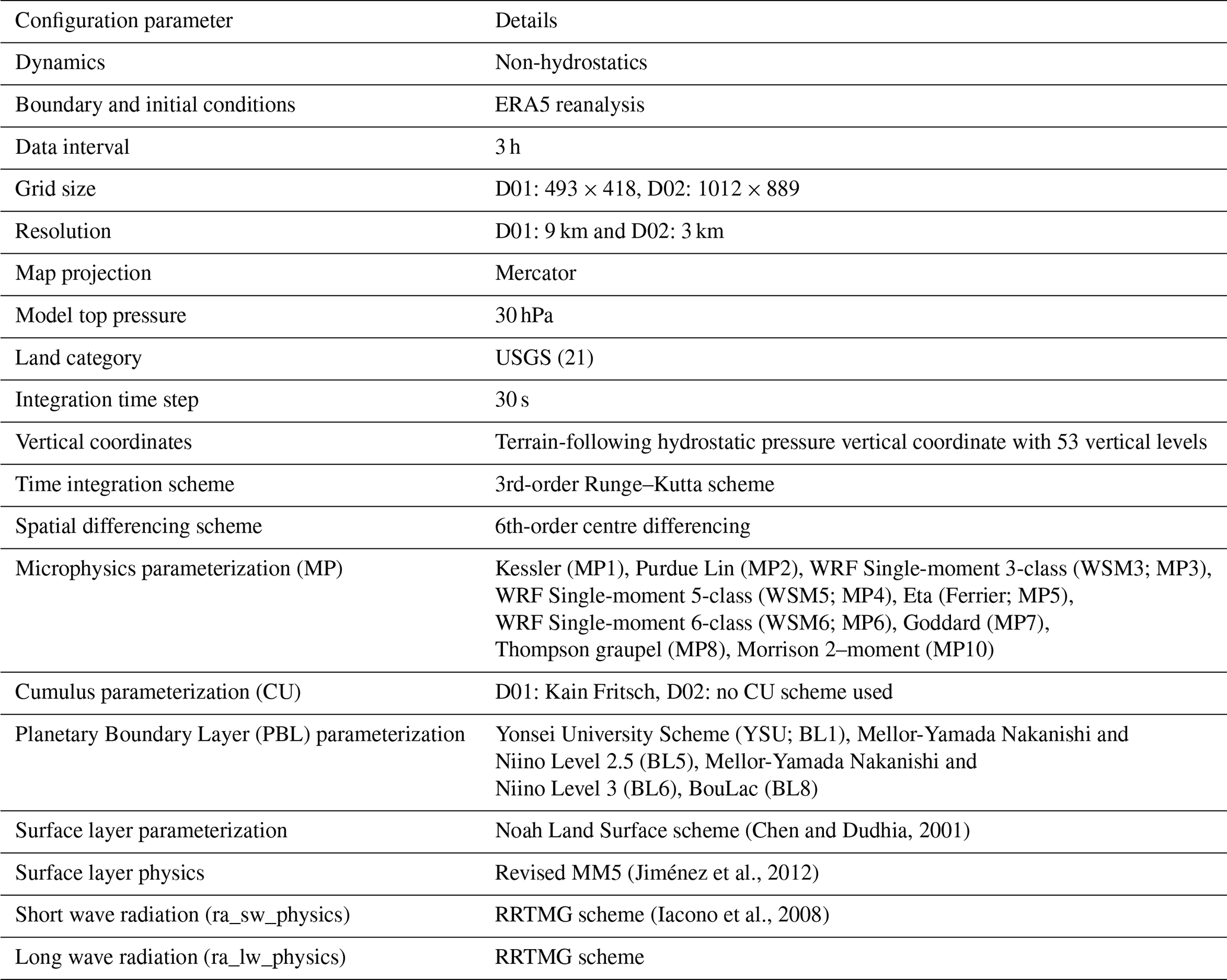
This study uses the WRF-ARW model version 4.4, a non-hydrostatic, fully compressible model with a terrain-following coordinate system (Skamarock et al., 2019). The model is configured with two-way nested domains with horizontal grid dimensions of 493 × 418 for the parent domain (D01) and 1012 × 889 for the nested domain (D02), and a model top pressure of 30 hPa, comprising 53 vertical hybrid sigma levels and a horizontal resolution of 3 km in the innermost domain, as shown in Fig. 1. The D01 domain covers a vast region of the AP from 21 to 65° E in the zonal direction and from 2 to 40° N in the meridional direction. We used a two-way nesting approach to allow feedback between the high-resolution inner domain and the coarser parent domain. This is essential for capturing small-scale processes like convection, PBL turbulence, and orographic effects, which can influence larger-scale circulation. The dynamic interaction improves physical consistency and is crucial for realistically simulating mesoscale convective systems (MCS) and associated rainfall. We conducted 612 simulations, spanning all 36 possible PBL-MP scheme combinations, to assess their joint performance across 17 EREs. Convection is explicitly resolved in D02, while D01 uses the Kain–Fritsch parameterization (Kain and Fritsch, 1993) for sub-grid convective processes (Snook et al., 2019).

We considered 36 combinations involving nine MP and four PBL schemes. The PBL schemes tested include Mellor-Yamada Nakanishi Niino (MYNN) Level 2.5 and Level 3 (BL5, BL6; Nakanishi and Niino, 2006), Yonsei University (YSU; BL1; Hong et al., 2006), and Bougeault-Lacarrère (BouLac; BL8; Bougeault and Lacarrere, 1989), while the MP schemes include Kessler (MP1; Kessler, 1969), Purdue Lin (MP2; Chen and Sun, 2002), WRF Single-Moment 3-class and 5-class (MP3 and MP4, respectively; Hong et al., 2004), Eta Ferrier, (MP5; Rogers et al., 2001), WRF Single-Moment 6-class (MP6; Hong and Lim, 2006), Goddard (MP7; Tao et al., 2016), Thompson (MP8; Thompson et al., 2008), and Morrison 2-Moment (MP10; Morrison et al., 2009). These combinations were selected based on their compatibility with the surface layer physics Revised MM5 scheme (Jiménez et al., 2012), and additional schemes were not included due to the higher computational and storage demands. Previous studies focusing on the AP have also utilized these schemes, including Deng et al. (2015), Attada et al. (2022), Luong et al. (2020), Schwitalla et al. (2020).

Initial and boundary conditions were extracted from ERA5 reanalysis data at 3 h intervals with a 0.25° resolution. All model simulations were conducted for 84 h, including a 48 h spin-up period to ensure model stability and reduce initialization biases. The analysis was focused on a 24 h window corresponding to the peak rainfall period of each ERE (Table 2). Our study specifically targets short-duration, event-based simulations of ERE. In such cases, the primary drivers are typically large-scale atmospheric instabilities and moisture advection rather than slower processes like land–surface interactions. Consequently, a 48 h spin-up period is sufficient to allow the model to dynamically and thermodynamically adjust to the initial and boundary conditions. Refer to Table 2 for the simulation start dates and Table 3 for the model configuration.

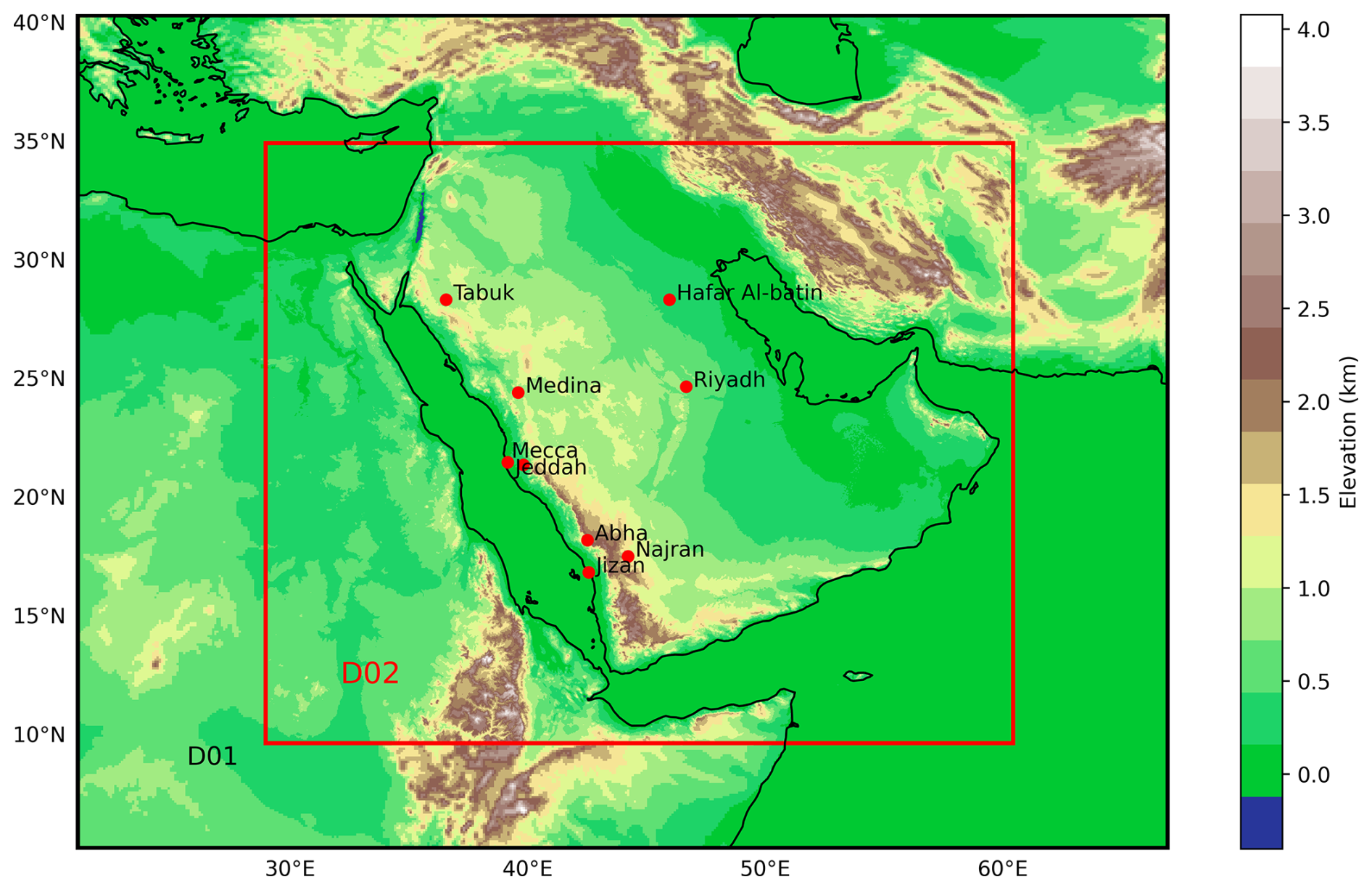
Figure 1 WRF-ARW domain for the AP region showing the elevation in the background. METAR locations are indicated with red markers.

Table 2 EREs across the AP selected to determine the performance of different MP and PBL scheme combinations. All simulation start times are at 00:00 UTC. IMERG-Final V07 rainfall values represent 24 h totals from simulation start for the 0.1° grid-cell with the highest amount for each ERE. Abbreviations: N = north, E = east, S = south, W = west, P = people.

(Chen and Dudhia, 2001)(Jiménez et al., 2012)(Iacono et al., 2008)

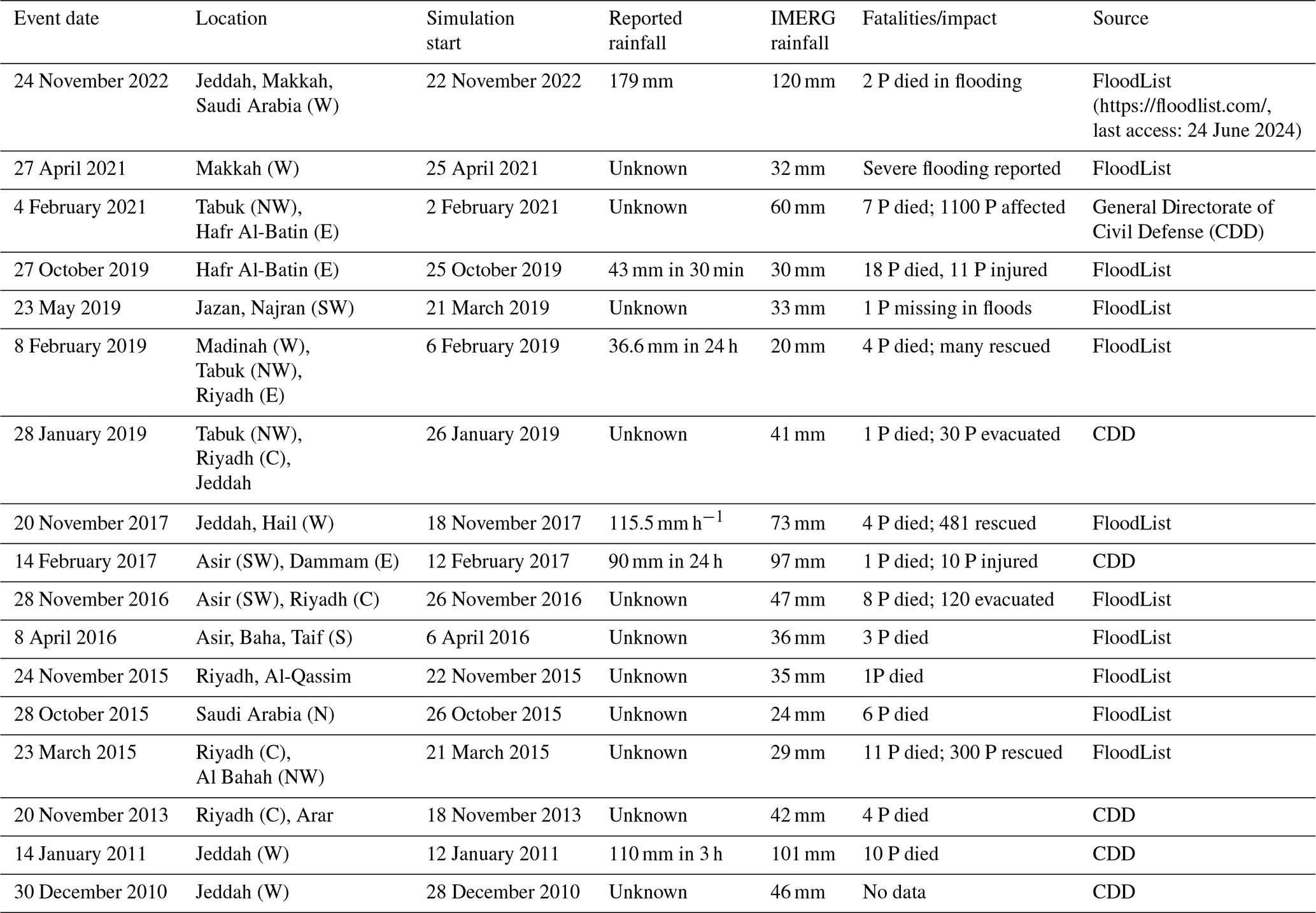
Table 3 WRF-ARW (Version 4.4) model configuration used in this study.

3.5 Model Assessment Approach

Each combination of MP and PBL schemes was extensively evaluated using the Kling–Gupta Efficiency (KGE; Gupta et al., 2009; Kling et al., 2012). The KGE is an aggregate performance metric that integrates correlation, bias ratio, and variability ratio into a single score, providing a holistic assessment of model performance. Several studies have successfully used KGE for spatial performance assessment of hydrometeorological models (e.g., Gupta et al., 2009; Patil and Stieglitz, 2015; Beck et al., 2019; Nguyen et al., 2022; Tudaji et al., 2025), supporting its application in our analysis. The formula for KGE is given by:

$$\begin{array}{}\text{(1)}& \text{KGE}=\mathrm{1}-\sqrt{(r-\mathrm{1}{)}^{\mathrm{2}}+(\mathit{\beta }-\mathrm{1}{)}^{\mathrm{2}}+(\mathit{\gamma }-\mathrm{1}{)}^{\mathrm{2}}},\end{array}$$

where r is Pearson's correlation coefficient between the observed and simulated data, β is the ratio of the mean simulated data to the mean observed data, assessing the bias, and γ is the ratio of the coefficients of variation of the simulated and observed data, evaluating the variability. A perfect but unattainable KGE score is 1, indicating complete agreement between simulated and observed data. A hypothetical simulation predicting only the observed mean would achieve a KGE of −0.41 (Knoben et al., 2019).

For rainfall, the KGE was calculated separately in space and in time. For the temporal KGE (Fig. 2), we first calculated, for each hour of the event day (Table 2), the spatial average of observed and simulated rainfall across D02 (Fig. 1). The KGE was derived from these 24 pairs of observed and simulated spatially averaged values. For the spatial KGE, for each grid cell within D02, the daily mean of observed and simulated rainfall was computed (Fig. S2). The KGE was subsequently calculated using these observed and simulated grid-cell daily means. To enable a consistent grid-cell-to-grid-cell comparison with IMERG-Final V07 observations, we resampled the WRF-ARW simulated rainfall data to the 0.1° IMERG grid using averaging. This resampling was performed using the xarray package in Python (Hoyer and Hamman, 2017).

Additionally, to determine whether the performance is significantly different between scheme combinations for rainfall, we calculated ΔKGE scores by subtracting the mean KGE across EREs from the KGE values, thereby eliminating systematic differences in scores among EREs. We then tested whether the distributions of ΔKGE values for different scheme combinations are statistically similar or different using pairwise independent t tests (Fig. S3). For 2 m air temperature, 2 m relative humidity, and 10 m wind speed, KGE was calculated from hourly METAR observations from the IOWA Mesonet and corresponding simulations from the nearest model grid-cell for the day of each ERE.

4 Results and Discussion

4.1 Which PBL scheme performs best in terms of rainfall?

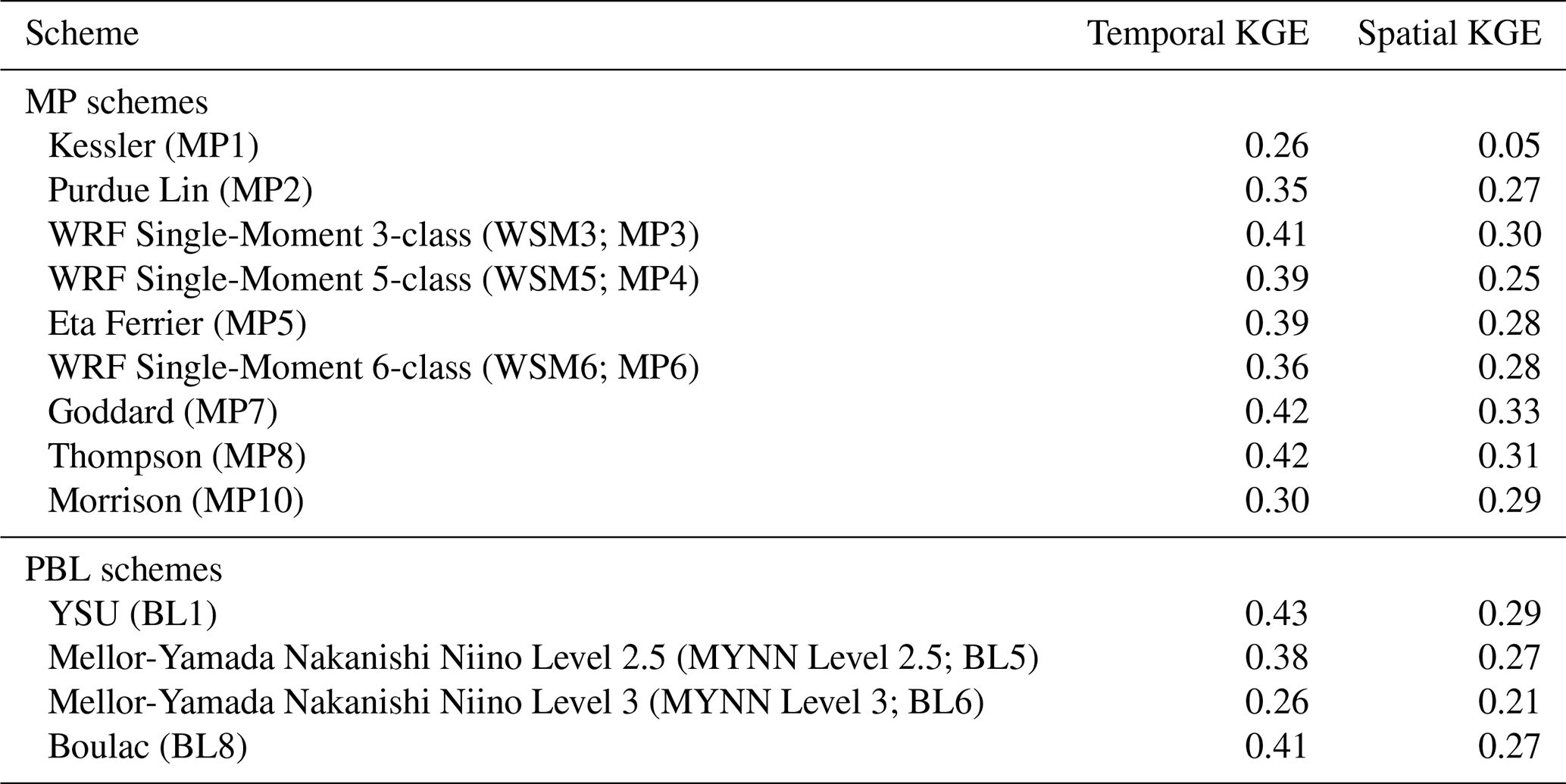
Figure 2 presents temporal KGE scores for 36 PBL-MP combinations across 17 EREs. As spatial KGE scores (Fig. S2) exhibit comparable patterns, the analysis here focuses on the temporal scores. The mean temporal and spatial KGE for the PBL schemes – BL1, BL5, BL6, and BL8 – are summarized in Table 4. Among these, the BL1 scheme showed superior performance among the PBL schemes (mean KGE of 0.43). Notably, BL1 is the only scheme with a non-local approach, unlike the other schemes, which are all local. This non-local mixing likely explains BL1's superior performance, enabling enhanced vertical mixing across the entire PBL. Non-local schemes like BL1 can represent large eddy structures and transport heat, moisture, and momentum over considerable vertical distances, a capability that is particularly crucial in arid environments with intense surface heating and sharp thermal gradients, such as Saudi Arabia (Hong et al., 2006; Hu et al., 2010). In contrast, local schemes like the BL5, BL6, and BL8 (mean KGE values of 0.38, 0.26, and 0.41, respectively) rely on gradients at specific vertical levels and small-scale turbulence, which restricts their ability to simulate deep convection and rapid vertical mixing.

Previous research has shown that non-local schemes, including BL1, yield a deeper and more accurately structured PBL than local schemes, especially in the presence of strong surface heating and convective activity, which are characteristic of desert climates (Xie et al., 2012; Cohen et al., 2015). Specifically, BL1's non-local treatment of PBL processes allows it to develop a deeper PBL during the daytime, a typical feature in arid regions, enhancing the scheme’s ability to capture severe convective activity (Cohen et al., 2015). The performance of BL1 in representing PBL processes is especially advantageous in regions where convection is often triggered by advancing frontal systems, as is common in the AP. In a case study using the WRF-ARW model, Cohen et al. (2015) demonstrated that BL1's non-local treatment improves the PBL's response to cold fronts, triggering convection more realistically and enhancing features like the formation of double lines of intense convection. This improvement arises because BL1 minimizes the dilution of moist air by dry air entrainment, maintaining a higher moisture concentration within the PBL. This “fuel” is crucial for sustaining severe convection when fronts initiate it, particularly in desert regions, where dry air entrainment can otherwise weaken or inhibit intense convective activity and thus reduce the accuracy of ERE simulations.

In contrast, local schemes like BL5 and BL6 and BL8 are optimized for stable or stratified PBLs, typically performing well by simulating small-scale turbulence. However, these schemes often struggle in unstable, highly convective environments like those in Saudi Arabia, where larger eddy structures dominate and require extensive vertical mixing to capture intense updrafts and rainfall (Hu et al., 2013; Cohen et al., 2015). Performance is particularly low for the BL6 scheme (mean KGE of 0.26; Table 4), sometimes showing negative KGE scores across different MP schemes (Fig. 2). The scheme's higher-order local closure approach can lead to over-diffusion, dampening essential vertical motions and limiting its ability to capture coherent eddies and large-scale vertical transport – critical for effective moisture and heat distribution needed for convective rainfall (Nakanishi and Niino, 2006; Shin and Hong, 2011).

Nevertheless, Schwitalla et al. (2020) reported the best performance with the MP8-BL5 scheme combination in their convection-permitting simulation over the AP for a single ERE on 14 July 2015 (Table 1), which contrasts with our findings. This contrast may be due to differences in the characteristics of that particular ERE, model setup, or surface properties. In particular, their use of a higher vertical resolution (100 levels) may have favored the performance of BL5, a local scheme that strongly depends on accurately resolved vertical gradients. Similarly, the relatively weaker performance of the BL6 and BL8 schemes in our simulations may be partly attributed to the coarser vertical resolution. However, unlike their single-event study, the present research evaluates 17 EREs across the AP spanning multiple seasons and years. This multi-ERE approach is particularly important for identifying parameterization schemes that are consistently reliable under a range of conditions. Since future climate projections cannot be directly validated against observations, selecting robust configurations based on a diverse set of past EREs is essential for improving model confidence in future applications.

4.2 Which MP scheme performs best in terms of rainfall?

Figure 2 presents temporal KGE scores for 36 PBL-MP combinations across 17 EREs. Since spatial KGE scores (Fig. S2) demonstrate similar values, the discussion is limited to temporal scores. The mean temporal and spatial KGE for various MP schemes, including MP1, MP2, MP3, MP4, MP5, MP6, MP7, MP8, and MP10, are presented in Table 4. The MP7 and MP8 schemes achieved the highest mean KGE scores. This is likely due to their sophisticated handling of cloud microphysics, especially in representing mixed-phase and ice-phase processes essential for simulating EREs in arid regions like Saudi Arabia. Though MP7 is a single-moment scheme, it includes detailed processes for ice, snow, and graupel, making it effective for capturing intense convective storms driven by complex thermodynamics and rapid cloud development (Tao, 2003). Its optimized treatment of rain formation and melting allows it to handle the rapid updrafts and temperature variations characteristic of desert climates, where efficient particle formation and fallout are crucial for high-intensity EREs.

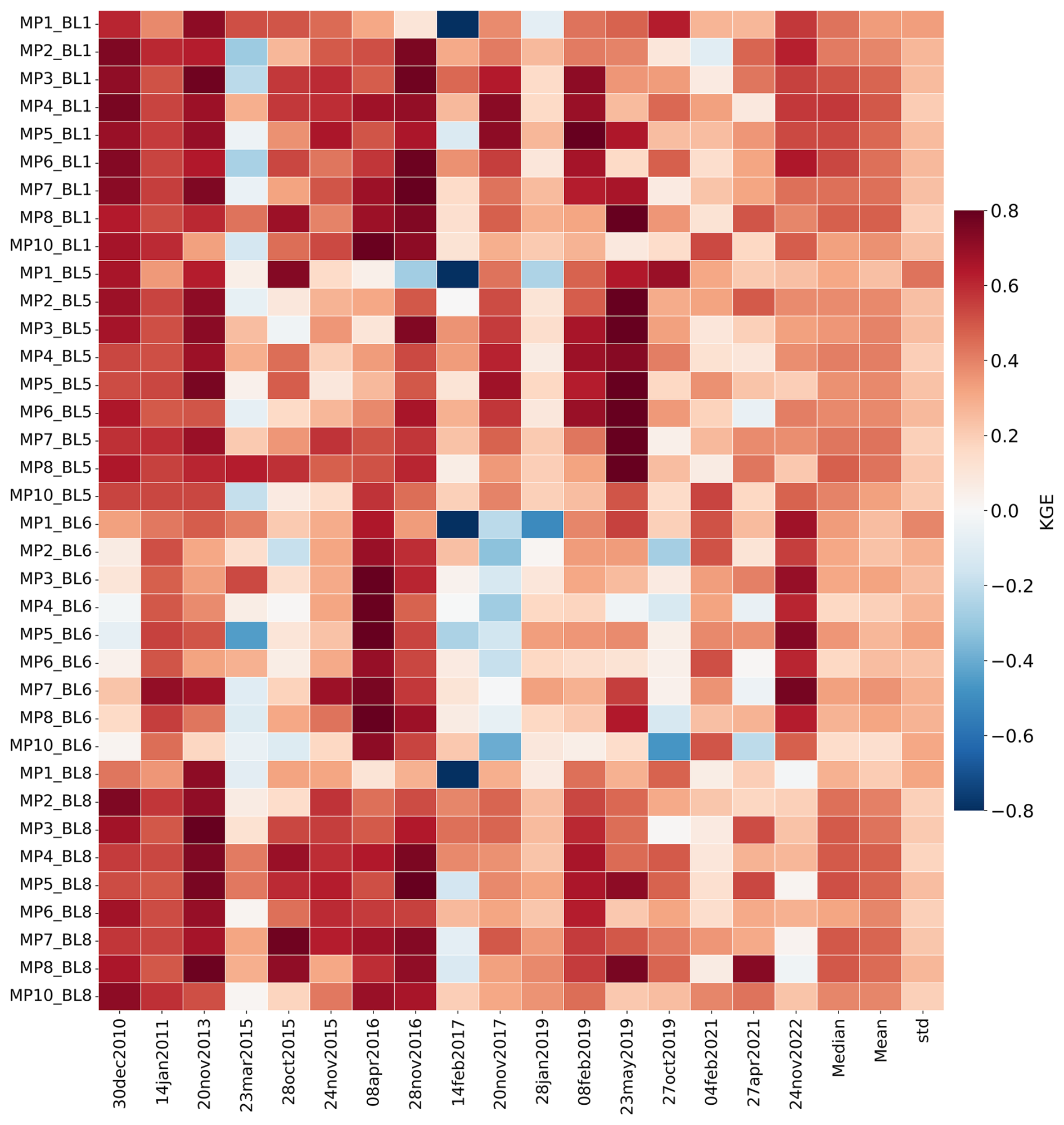
Figure 2 Temporal KGE scores for rainfall derived from 36 WRF-ARW scheme combinations across 17 EREs. The scores were calculated by comparing hourly WRF-ARW simulated rainfall against IMERG-Final V07 satellite rainfall data over the event day.

Table 4 Mean KGE values across all simulations for temporal and spatial assessments of MP and PBL schemes.

As a double-moment approach, the MP8 scheme further enhances these capabilities by dynamically adjusting particle size distributions, including cloud droplets, rain, ice and snow. This adaptability allows it to respond effectively to environmental changes typical of desert frontal systems, where intense updrafts can quickly alter particle sizes (Thompson et al., 2008). The double-moment structure offers flexibility in tracking a broad range of particle sizes, enabling MP8 to simulate light and heavy rainfall effectively. This capability is crucial in arid regions, where rapid shifts between intense rainfall and dry conditions are common, and tracking both mass and concentration enhances the accuracy of these transitions.

The superior performance of these schemes over simpler single-moment models, like MP1, MP2, or MP3 underscores the importance of advanced microphysical processes – including graupel and hail processes, multiple ice-phase species, prognostic treatment of various hydrometeors, and more complex interactions between cloud and rainfall particles – for capturing ERE variability and intensity. Simpler schemes lack adaptability to evolving particle size distributions, limiting their effectiveness in highly convective environments with rapid shifts. Notably, despite its advanced double-moment structure, Morrison underperformed, possibly due to interactions with other model components that may hinder accuracy in arid, convective conditions – a point warranting further research beyond this study. Overall, our results highlight the importance of selecting MP schemes with detailed ice and mixed-phase processes when modeling EREs in desert regions.

4.3 Which component of the Kling–Gupta Efficiency (KGE) affects the final rainfall scores the most?

Figure 3a presents the values of KGE and its components – correlation, bias, and variability (r, γ, and β, respectively; Eq. 1) – for all 17 EREs for the best performing MP8_BL1 scheme combination for rainfall (Fig. 2 and Table 4). In the interest of conciseness, we focus only on the temporal KGE results here, as the spatial KGE results are quite consistent (see Sect. 4.1, 4.2, and 4.5, and Table 4).

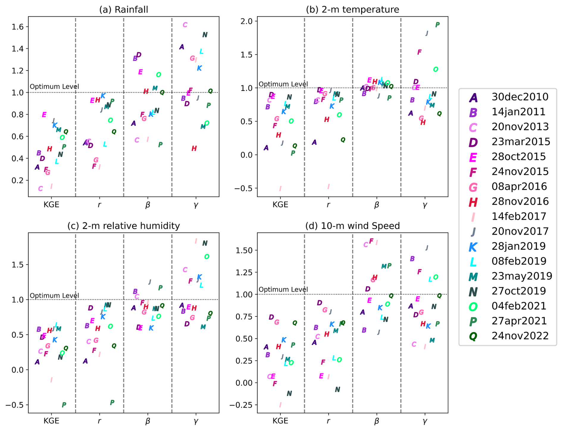
Figure 3 Correlation coefficient (r), bias (β), and variability ratio (γ) values used to calculate the KGE values for the best-performing combination across 17 EREs for (a) Rainfall, (b) 2 m air temperature, (c) 2 m relative humidity, and (d) 10 m wind speed. Panel (a) uses IMERG-Final V07 as reference and panels (b)–(d) METAR observations over each 24 h event day. The letters (A, B,..., Q) indicate the 17 different EREs (Table 2).

Correlation is sensitive to the timing of EREs, variability ratio is sensitive to the distribution, and bias reflects the mean. For the best combination (MP8_BL1), the mean temporal KGE score for rainfall across 17 EREs is 0.48. Decomposing this score into the three components, expressed as $|r-\mathrm{1}|$, $|\mathit{\beta }-\mathrm{1}|$ and $|\mathit{\gamma }-\mathrm{1}|$ to make them comparable, yields mean absolute values of 0.33, 0.23, 0.25, respectively, where values closer to 0 indicate better performance. Among the three KGE components, the scheme thus performed worst in terms of correlation, and this subcomponent thus exerted the dominant influence on the final KGE scores. This suggests that in order to get an improved KGE score, the most important component score to improve is the correlation, which, in the temporal assessment, is related to the timing of EREs. The mean KGE value across all other schemes and EREs is 0.36, and the mean values for $|r-\mathrm{1}|$, $|\mathit{\beta }-\mathrm{1}|$ and $|\mathit{\gamma }-\mathrm{1}|$ are 0.34, 0.29, and 0.24, respectively. This suggests that the correlation also tends to exert the dominant influence for the other scheme combinations, while bias also plays a role. The mean KGE score for the worst-performing scheme combination MP10_BL6 is 0.13, while the mean values of the three KGE components $|r-\mathrm{1}|$, $|\mathit{\beta }-\mathrm{1}|$, and $|\mathit{\gamma }-\mathrm{1}|$ are 0.33, 0.57, and 0.36, respectively. This scheme thus performs particularly poorly in terms of bias.

4.4 How statistically significant are the differences in performance among scheme combinations in terms of rainfall?

The differences in KGE between different scheme combinations for rainfall are generally relatively small. For example, the best-performing scheme combination (MP8_BL1) achieved a mean KGE of 0.48, while the second-best-performing scheme combination (MP7_BL1) achieved a mean KGE of 0.44 (Fig. 2). Furthermore, the corresponding standard deviations across EREs are 0.20 and 0.24, respectively, indicating substantial variability in scores among EREs. Additionally, the consistency in performance ranking among EREs is fairly low (Fig. 5). This raises the question whether the observed differences in performance between scheme combinations are statistically significant and, hence, whether our evaluation approach is adequate for determining the relative performance of different scheme combinations, which is the primary objective of this study.

Figure 4 presents a 36×36 matrix of pairwise p values from independent t tests comparing ΔKGE distributions of 36 scheme combinations for rainfall. ΔKGE values were calculated by subtracting the mean KGE across EREs from the KGE values presented in Fig. 2, thereby eliminating systematic differences in scores among EREs. The results reveal that the best-performing scheme combination (MP8_BL1) significantly outperforms 21 other scheme combinations (at p < 0.1), whereas the worst-performing scheme combination (MP10_BL6) performed significantly worse than 28 other scheme combinations (also at p < 0.1). These results confirm that our assessment provides meaningful and statistically significant insights into the relative performance of different scheme combinations. However, our assessment does not definitively identify a single best-performing scheme but instead highlights groups of better- and worse-performing schemes.

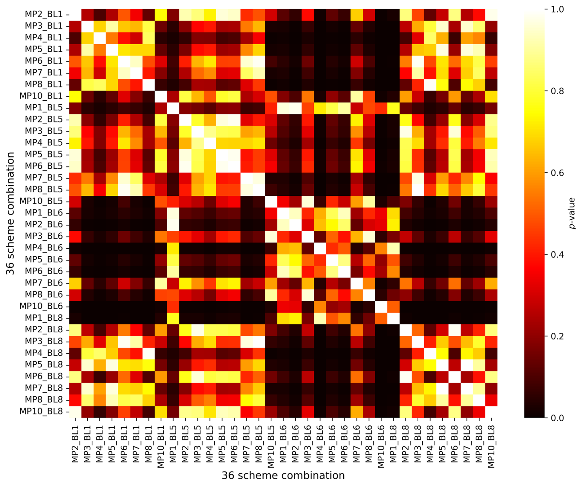
Figure 4 Pairwise p values from independent t tests comparing the ΔKGE distributions of 36 scheme combinations for rainfall. ΔKGE values were calculated by subtracting the mean KGE across EREs from the KGE values presented in Fig. 2. A p threshold of 0.1 was used to identify statistically significant differences between scheme combinations.

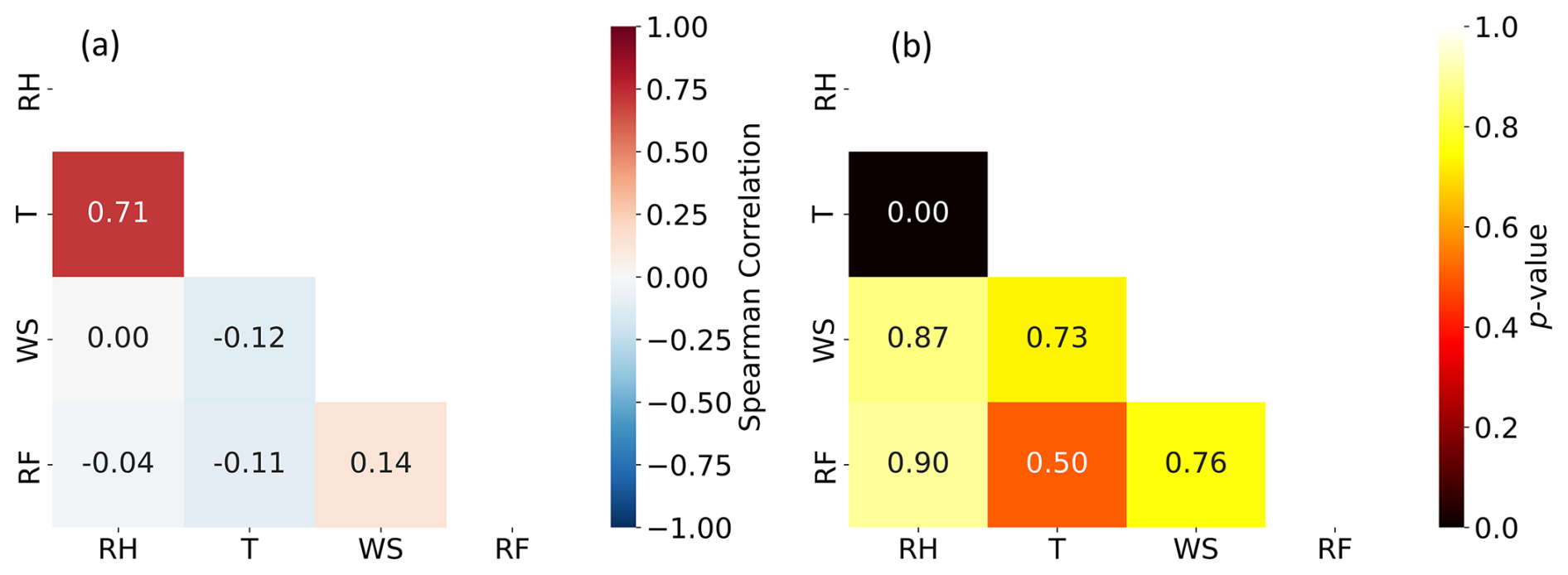
Figure 5 (a) Mean Spearman correlation coefficients and (b) corresponding median p values calculated among mean KGE scores for different meteorological variables, indicating the degree of consistency in performance rankings among variables. Variable definitions: 2 m relative humidity = RH; 2 m air temperature = T; 10 m wind speed = WS; and rainfall = RF.

The ability of an assessment such as this to detect significant differences in performance between schemes depends on the mean and standard deviation of the ΔKGE distribution. Assuming a standard deviation of 0.15 (equivalent to that of MP8_BL1), the current sample size of 17 EREs requires a mean ΔKGE difference greater than 0.06 between schemes to yield a statistically significant difference at p < 0.1. Analyzing a larger sample of EREs would reduce the required mean difference, making it easier to detect significant differences in performance between schemes. For example, if we were to analyze 50 EREs, the required difference in mean ΔKGE would be just 0.03 (assuming again a standard deviation of 0.15). However, analyzing a larger number of EREs is computationally more expensive.

The standard deviation (i.e., the variability in ΔKGE among EREs) and hence the number of EREs required to detect significant performance differences between schemes are partly influenced by the quality of the reference data. In this study, we used a microwave satellite-based rainfall product (IMERG-Final V07), which is associated with greater uncertainty than gauge-radar-based datasets (Beck et al., 2019). This increased uncertainty may have contributed to higher variability in KGE scores (Evans and Imran, 2024). Unfortunately, radar data are only commercially available in Saudi Arabia. Due to the strong correlation between different microwave satellite-based rainfall datasets – such as IMERG, GSMaP (Kubota et al., 2024), and CMORPH (Xie et al., 2019) – and the fact that IMERG-Final V07 significantly outperforms other satellite datasets (Wang et al., 2025), we were unable to quantify the uncertainty arising from the choice of reference data as done by Evans and Imran (2024).

4.5 How consistent are the temporal and spatial performance assessments for rainfall?

We calculated KGE scores both temporally and spatially to assess the performance of the 36 PBL-MP scheme combinations across the 17 EREs. The temporal KGE results for rainfall are presented in Fig. 2, while the spatial KGE results for rainfall are provided in Fig. S2. The mean KGE values categorized by MP and PBL schemes, for both temporal and spatial assessments, are summarized in Table 4. The overall mean temporal KGE across all schemes and EREs for rainfall is 0.37, whereas the overall mean spatial KGE is 0.26. This indicates that the simulations are more effective at capturing temporal variations in rainfall than spatial variations. This is expected, as accurately simulating the location of localized convective systems remains a major challenge. Overall, we found a strong consistency in the overall ranking of schemes between the temporal and spatial assessments, with a Spearman rank correlation of 0.65 (p < 0.001) between the mean temporal and spatial KGE values for the scheme combinations. The MP7 and MP8 schemes, when combined with BL1, consistently ranked highest across both temporal and spatial KGE assessments (Figs. 2 and S2; Table 4). Conversely, the MP1 scheme with BL6 scheme performed worst in both assessments.

4.6 How consistent is the performance ranking among different variables?

Ideally, if our conclusions about the performance of various MP and PBL scheme combinations regarding rainfall are valid, and if this superior performance truly reflects a model that better represents reality (i.e., we are getting the right results for the right reasons; Kirchner, 2006), then the performance ranking for rainfall should align with those of the other variables (2 m air temperature, 2 m relative humidity, and 10 m wind speed). Indeed, for all variables, MP8_BL1 provided the highest mean temporal KGE (Fig. 2 and Table 4), tentatively suggesting that this particular scheme combination does indeed yield a more robust model in all respects.

Additionally, we calculated Spearman rank correlations and corresponding p values between the temporal mean KGE scores for the different variables (Fig. 5), to examine the degree of consistency in performance rankings among the variables. Most variable pairs exhibited insignificant correlations except for temperature and relative humidity, which are intrinsically linked through the Clausius–Clapeyron relationship as temperature controls saturation vapor pressure and, thus, relative humidity. The lack of significant correlations might have three potential explanations. First, uncertainties in the reference data may cause discrepancies in model performance; the significant uncertainty in IMERG for rainfall (Wang et al., 2025), along with the difficulty of comparing point-based IOWA Environmental Mesonet data to WRF-ARW grid cells for other variables, makes this explanation plausible. Second, although MP and PBL schemes strongly influence rainfall simulation, other model components like land surface schemes, which affect soil moisture and heat fluxes, and radiation schemes, which affect surface and atmospheric energy balances, may have a more pronounced impact on variables such as temperature and wind speed. Third, there might be compensatory behavior within the model, where improvements in simulating one variable do not necessarily result in a more realistic simulation and may yield reduced performance in others.

This phenomenon, where models achieve the right results for the wrong reasons, is not uncommon in geosciences and poses significant challenges in model evaluation and improvement (Kirchner, 2006; Parker, 2006; Knutti, 2010; Hourdin et al., 2017; Broecker, 2017; Krantz et al., 2021). Resolving this requires examining model structure and variable interactions more closely to determine if improvements reflect real accuracy or trade-offs, which is beyond the scope of the current study.

4.7 What do the spatial patterns in simulated and observed rainfall look like for the EREs?

Figures 6 and 7, respectively, present observed (IMERG-Final V07) and simulated (WRF-ARW) 24 h rainfall accumulations for the 17 selected EREs. The WRF-ARW model simulations were generated using the best-performing scheme (MP8_BL1). Overall, WRF-ARW generally seems to capture reasonably well the location, extent, and amounts indicated by IMERG. For example, the strong convective systems with high-intensity localized rainfall exceeding 120 mm on EREs like 20 November 2013 and 28 January 2019 are captured well. However, the model overestimates rainfall for several EREs (e.g., 8 February 2019) and underestimates rainfall for others (e.g., 28 October 2015). While WRF-ARW generally captures the broad patterns, the lack of a better match is attributable to several reasons. First, potential deficiencies in the MP, BL, and convection schemes, along with other modeling limitations, can lead to inaccuracies in moisture convergence and convective updrafts (Taraphdar et al., 2021; Attada et al., 2022). These limitations include simplified representations of land–atmosphere interactions, unresolved sub-grid processes, and the use of prescribed lateral boundary conditions updated every 6 h, which may not fully capture fast-evolving or small-scale features entering the domain. Second, we used ERA5 as boundary conditions to force the model, and while ERA5 is the best reanalysis currently available, it nonetheless is subject to random errors and bias (Hersbach et al., 2020; Soci et al., 2024). Third, we did not include data assimilation or nudging (Lei and Hacker, 2015; Feng et al., 2021), two important techniques to improve the simulations. Fourth and finally, the IMERG data, though found to perform relatively well in precipitation product evaluations (Abbas et al., 2025; Wang et al., 2025), nonetheless carries significant uncertainty in the region.

Figure 6 Daily accumulated rainfall from our observation-based data source (IMERG-Final V07) for the 17 EREs. The white areas indicate grid cells with daily rainfall < 0.1 mm.

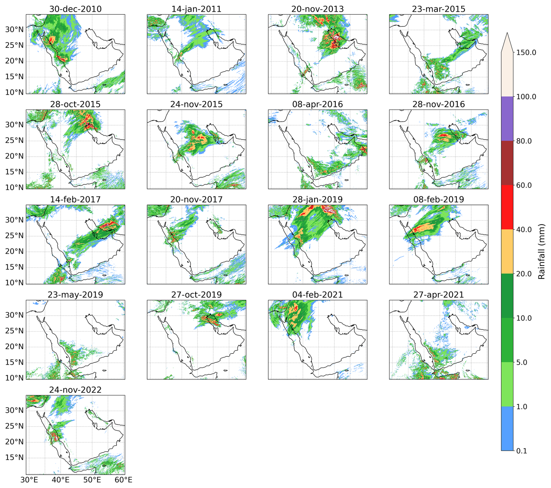
Figure 7 Daily accumulated rainfall from WRF-ARW using the best-performing scheme combination (MP8_BL1) for the 17 EREs. The white areas indicate grid cells with rainfall < 0.1 mm.

4.8 How well does the model perform in terms of the other variables?

While the previous subsections focused primarily on rainfall, it is worthwhile to investigate how the model performs in terms of other meteorological variables. To this end we analyzed the KGE components for 2 m air temperature, 2 m relative humidity, and 10 m wind speed as presented in Fig. 3b, c, and d, respectively. Fig. 3b presents the KGE and its components (r, γ, and β) for all 17 EREs for temperature using the best-performing combination (MP8_BL1). For this scheme, the mean temporal KGE score across the 17 EREs is 0.47, which is similar to that obtained for rainfall (0.48). This is somewhat unexpected, as temperature is constrained by surface energy balance processes, resulting in smoother variations and less extreme variability compared to rainfall. The mean values for $|r-\mathrm{1}|$, $|\mathit{\beta }-\mathrm{1}|$ and $|\mathit{\gamma }-\mathrm{1}|$ for temperature are 0.32, 0.06, and 0.33, respectively. Among the three KGE components, the scheme thus performed worst in terms of correlation and variability, which therefore exert the dominant influence on the final KGE scores.

Figure 3c presents the KGE and its components for the 17 EREs for relative humidity using the best performing scheme (MP8_BL1). For this scheme, the mean temporal KGE score across 17 EREs is 0.31, which is lower than that obtained for rainfall and temperature. This may reflect relative humidity's nonlinear dependence on both temperature and moisture in addition to the high spatio-temporal variability. The mean values for $|r-\mathrm{1}|$, $|\mathit{\beta }-\mathrm{1}|$ and $|\mathit{\gamma }-\mathrm{1}|$ are 0.47, 0.18, 0.33, respectively. Among the three KGE components, the scheme thus performed worst in terms of correlation, followed by variability, which therefore exert the dominant influence on the final KGE scores.

Figure 3d presents the KGE and its components for the 17 EREs for wind speed using the best performing scheme (MP8_BL1). For this scheme, the mean temporal KGE score across the 17 EREs is 0.29, the lowest among the four variables, likely due to the influence of fine-scale topography and surface roughness variability on wind speed (Branch et al., 2021). The mean values for $|r-\mathrm{1}|$, $|\mathit{\beta }-\mathrm{1}|$ and $|\mathit{\gamma }-\mathrm{1}|$ are 0.52, 0.28, 0.30, respectively. Among the three KGE components, the scheme thus performed worst in terms of correlation, which therefore exerts the dominant influence on the final KGE scores.

4.9 How do the PBL and MP schemes used in previous studies compare with those identified as optimal in our evaluation?

Although our findings are subject to uncertainty and must be interpreted with caution, as highlighted in the previous subsections, they provide a useful basis for evaluating schemes used in previous WRF-ARW studies in the region. Our review of these studies (Table 5) reveals varying choices of PBL and MP schemes, with mixed alignment to the results of this study. Several studies, such as those by Abida et al. (2022), Almazroui et al. (2018), and Patlakas et al. (2023), used the BL1 scheme, which our results confirm as the best-performing scheme for capturing the unique convective dynamics in arid climates. These studies highlighted BL1's robust vertical mixing capabilities and adaptability to desert environments. On the other hand, studies like Attada et al. (2020) and Taraphdar et al. (2021), which employed BL6 and QNSE (BL4), respectively, used local turbulence schemes that our findings show may be less suited for unstable, highly convective conditions typical in the region. Similarly, while MP schemes like MP8 and MP7, identified in our study as well-performing, were used in some cases (Taraphdar et al., 2021; Attada et al., 2020), other studies, such as Deng et al. (2015), relied on simpler MP schemes like MP2 and MP5, which may lack the sophistication needed to capture mixed-phase processes in intense convective systems fully. Thus, while several studies employed schemes previously shown to perform well in similar regional contexts, others might have improved simulation accuracy by incorporating the BL1 scheme and advanced MP schemes identified as effective in our study. However, we would like to reiterate that our findings are subject to uncertainty, and these conclusions should therefore be interpreted with caution.

Luong et al. (2020)Francis et al. (2024)Deng et al. (2015)Attada et al. (2020)Taraphdar et al. (2021)Abida et al. (2022)Almazroui et al. (2018)Patlakas et al. (2023)

Table 5 Studies simulating EREs in the Middle East using WRF-ARW.

5 Conclusion

This study evaluated the performance of PBL and MP parameterizations for simulating EREs in the AP using the WRF-ARW model at a convection-permitting resolution, serving as a verification study for hydrometeorology in the region. The results show that the model captures temporal rainfall variations (mean KGE = 0.37) more effectively than spatial patterns (mean KGE = 0.26), reflecting the localized nature of rainfall in the region. Nonetheless, a strong correlation (Spearman rank correlation of 0.65, p < 0.001) between temporal and spatial KGE rankings highlights consistency in scheme performance. This verification is crucial for improving confidence in hydrometeorological modeling and forecasting, particularly for regions prone to flash floods and extreme rainfall. Thus, the findings guide model selection and a vital validation benchmark for future hydrometeorological research and operational forecasting in desert climates.The answers to the questions, each addressed in detail in the Results and Discussion, are as follows:

• a.

  Which PBL scheme performs best in terms of rainfall?
  
  The BL1 scheme outperformed the other PBL schemes, achieving a mean temporal KGE of 0.43 and a mean spatial KGE of 0.29. This superior performance is attributed to non-local mixing, which enhances vertical transport and convective processes and makes it particularly effective for simulating ERE in arid regions like the AP. In contrast, local schemes such as BL5, BL6, and BL8 performed worse because they rely on small-scale turbulence, which limits the representation of deep convection.

• b.

  Which MP scheme performs best in terms of rainfall?
  
  The MP7 and MP8 schemes performed best, achieving a mean temporal KGE of 0.42, with mean spatial KGEs of 0.33 and 0.31, respectively. Their strong performance is attributed to their advanced mixed-phase and ice-phase microphysics. MP8's double-moment structure enhances adaptability, while MP7's optimized ice and graupel processes improve convective simulations. These results highlight the benefit of advanced MP schemes for accurately modeling EREs in arid regions.

• c.

  Which component of the Kling–Gupta Efficiency (KGE) affects the final rainfall scores the most?
  
  Among the three KGE components (correlation, bias ratio, and variability), correlation and variability exerted the strongest influence on the temporal rainfall KGE scores. Enhancing these components should be prioritized to further improve the accuracy of ERE simulations.

• d.

  How statistically significant are the differences in performance between scheme combinations in terms of rainfall?
  
  Pairwise statistical tests between distributions of temporal KGE scores obtained by the scheme combinations revealed that the MP8_BL1 combination significantly outperformed 21 other scheme combinations, while the poorest-performing combination, MP10_BL6, was statistically inferior to 28 other combinations. Thus, we could not statistically identify a single best- or worst-performing combination, despite the large sample of 17 EREs.

• e.

  How consistent are the temporal and spatial performance assessments for rainfall?
  
  The assessment reveals that MP7_BL1 and MP8_BL1 performed best in both the temporal and spatial assessment for rainfall. The higher mean temporal KGE (0.37) compared to the mean spatial KGE (0.26) for all 36 combinations indicates that the model captures rainfall variability more effectively over time than across space. Although spatial KGE values were lower, the ranking of combination performance remained consistent (Spearman rank correlation of 0.65).

• f.

  How consistent is the performance ranking among different variables?
  
  The MP8_BL1 combination provided the best performance for all variables (rainfall, 2 m air temperature, 2 m relative humidity, and 10 m wind speed). However, we obtained weak correlations between performance rankings across the variables, indicating poor consistency. This is likely because different physical processes govern the simulations of different variables. That is, while MP and PBL schemes influence rainfall, other components, such as land surface and radiation schemes, affect temperature and wind. This underlines the complexity of model parameterization, particularly as cloud evolution is influenced not only by PBL and MP schemes but also by radiative processes, emphasizing the need for further integrated research.

• g.

  What do the spatial patterns in simulated and observed rainfall look like for the EREs?
  
  For the best-performing physics combination (MP8_BL1), the spatial patterns of simulated and observed rainfall were generally well captured, although occasional overestimations and underestimations were noted. These discrepancies are likely attributable to limitations in the boundary conditions (the ERA5 reanalysis) and uncertainties in the observations (the IMERG-Final V07 satellite-based rainfall product).

• h.

  How well does the model perform in terms of the other variables?
  
  Using the best-performing scheme combination (MP8_BL1), air temperature showed a mean temporal KGE score of 0.47, similar to that of rainfall (0.48), with performance limited mainly by correlation and variability. Relative humidity had a lower mean temporal KGE score (0.31), like due to its nonlinear dependence on temperature and moisture, with correlation as the dominant error source. Wind speed had the poorest performance (mean temporal KGE of 0.29), likely due to unresolved fine-scale topographic and surface roughness effects.

• i.

  How do the PBL and MP schemes used in previous studies compare with those identified as optimal in our evaluation?
  
  Our findings align with several previous studies in the Middle East that employed the BL1 scheme, reinforcing its effectiveness for simulating regional atmospheric dynamics. At the same time, our results suggest that studies using simpler MP schemes – such as MP2 or MP5 – may achieve improved simulation accuracy by adopting more advanced schemes like MP8.

By identifying the optimal PBL and MP combination from 36 tested configurations across 17 EREs, we established a strong foundation for improving the accuracy of ERE simulations across the AP, a region that remains understudied despite frequent flash floods and significant casualties. As the most comprehensive evaluation of PBL and MP schemes in the AP to date, our study emphasizes the importance of parameterization choices on ERE simulation performance, serving as a key reference for future modeling efforts. Our results may guide researchers and forecasters in selecting the most effective parameterization schemes, ultimately contributing to more reliable forecasting and enhanced disaster preparedness in arid environments. To further advance ERE simulation fidelity, future work should extend beyond PBL and MP schemes to systematically evaluate the impact of land surface schemes, radiation parameterizations, and data assimilation techniques.