Assessing extreme total water levels across Europe for large-scale coastal flood analysis

Coastal storm-induced flooding threatens millions of people and infrastructures, highlighting the need for comprehensive flood risk assessments. A key component of these assessments is the spatial characterization of total water level (TWL), the primary driver of coastal flooding. We propose a flexible methodology for developing large-scale TWL hindcasts to estimate extreme events, considering possible spatial variabilities in marine dynamics. This methodology is applied to the European coastline, integrating downscaled nearshore waves, storm surges, and tides. The resulting hourly time series of the TWL have a spatial resolution of 1 km and covers the period from 1985 to 2021. Spatial variability is considered in foreshore slopes and extreme value detection thresholds, addressing common simplifications in large-scale studies. In addition to a characterization of extreme events based on the relative contributions of TWL components, sensitivity analyses of the wave contribution, wave data resolution, foreshore slopes, and wave setup formulations are conducted. The tide-dominated Atlantic coast is where the TWL is most affected by the wave dataset. The storm surge-dominated Baltic region exhibits the lowest confidence in estimating TWL return levels, partially due to the data and methods used. The Mediterranean Sea, characterized as a mixed environment, is the most sensitive to the inclusion of wave contribution. A classification of TWL extremes revealed that no regions have extreme events dominated by wave setup when compared to the remaining components, while those dominated by tides show the highest return levels.

1 Introduction

The assessment of coastal impacts resulting from extreme coastal flooding events is essential for understanding and mitigating associated potential risks (Neumann et al., 2015). These risks include, among others, damage to coastal infrastructure and the built environment, as well as impacts on the population and ecosystems (Barnard et al., 2019; Rashid et al., 2021; Rasmussen et al., 2022). The total water level (TWL) is the most commonly used indicator in coastal flooding studies. It is frequently used as a forcing variable for flood models aimed at generating maps of flood extent and depth. Accurate coastal flood estimates require that TWL includes a proper spatial characterization of all relevant components (i.e., waves, storm surges, and astronomical tides) (Cabrita et al., 2024; Kirezci et al., 2020; Pugh, 1987). However, estimating extreme TWL at coastal locations becomes increasingly complex as the spatial scale of the study domain increases.

One key challenge lies in the method used to reconstruct the TWL, which requires the selection and characterization of relevant components at appropriate spatial and temporal scales. We consider TWL as a combination of astronomical tide, storm surge, and a contribution by ocean waves (usually the wave setup) (Pugh and Woodworth, 2014). Among these, assessing the contribution of waves is particularly critical, as it involves evaluating nearshore wave conditions and the associated wave setup, which depending on the formulation can be influenced by the foreshore slope. A second key challenge concerns the choice of an extreme value modeling approach to characterize extreme events in terms of probability of occurrence. Each stage in this process introduces uncertainty, from data selection and the formulation used to calculate wave contributions to TWL, to the definition of extreme events (e.g., threshold selection) and the fitting of statistical distributions to estimate return levels (Hinkel et al., 2021; Toimil et al., 2020).

Initial attempts at assessing coastal flood impacts at large scales relied on the DIVA model (Vafeidis et al., 2008), which provided TWL and return level scenarios. More recent efforts have focused on improving the spatial resolution and temporal extent of large-scale TWL hindcasts. For example, TWL has been globally reconstructed from 1993 to 2013 at a 111 km resolution (Vitousek et al., 2017), from 1979 to 2014 at 70 km resolution (Kirezci et al., 2020), and from 1993 to 2015 at 50 km resolution (Almar et al., 2021). For the European coastline, TWL from 1979 to 2014 was calculated at 25 km resolution (Vousdoukas et al., 2016), and from 2010 to 2019 at 2.5 km resolution (Le Gal et al., 2023).

With respect to TWL components, storm surges and astronomical tides are commonly included in flooding studies, whereas the wave component is often neglected despite its potential importance along many coasts (Muis et al., 2015, 2016; Paprotny et al., 2016, 2018). At large scales, few studies include wave effects, which may take different forms depending on the processes considered. These include: (1) static wave setup, defined as the superelevation of the coastal water surface due to wave breaking; (2) dynamic wave setup which adds the effect of the infragravity swash to the static wave setup; and (3) wave runup, which further includes the incident swash component (Stockdon et al., 2006). While the estimation of infragravity swash remains uncertain at large scales, incident swash generally does not sustain flooding capable of causing coastal damage (Hinkel et al., 2021). For two-dimensional flood modeling, the wave contribution component is usually represented by the static wave setup (hereafter referred to as wave setup). Several methods exist for estimating wave setup at large scales. The most widely used is the empirical approach proposed by Guza and Thornton (1981), which estimates wave setup as a fraction of the significant wave height (Hs), namely 0.2Hs. However, this method often leads to the overestimation of wave setup (Hinkel et al., 2021). More accurate alternatives involve simplified parameterizations. For instance, the semi-empirical formulation by Stockdon et al. (2006) has been adopted globally (Rueda et al., 2017; Vitousek et al., 2017), as well as the Shore Protection Manual method (Kirezci et al., 2020; USACE, 1984). One way these parameterizations improve accuracy is by incorporating nearshore bathymetry, particularly the foreshore slope (Dodet et al., 2019; Gomes da Silva et al., 2020).

A limitation within the use of wave parameterizations lies in accurately characterizing the foreshore slope at large scales. Despite its importance, this parameter remains difficult to quantify, which limits its practical applicability in many coastal assessments. Consequently, some authors applied a constant slope of 1 : 30 (Kirezci et al., 2020), while others used a wave setup formulation designed for dissipative beaches (Vitousek et al., 2017), that does not require slope data (Stockdon et al., 2006). Alternatively, a method developed by Sunamura (1984) allows for the estimation of spatially and temporally varying foreshore slopes based on wave conditions. Compared with locally observed slopes and globally constant values, this method accounts for morphological feedback, given that evolving beach morphology can influence wave contributions to sea level, as considered in Sunamura's formulation (Melet et al., 2020).

Another limitation in these studies is that offshore wave conditions are often used, despite their coarse resolution and limited suitability for accurately assessing coastal impacts. More precise estimates of coastal flooding require nearshore wave data, which better capture the relevant coastal dynamics, as wave setup is not an offshore process (Dodet et al., 2019). The use of nearshore information is however limited at large geographical scales due to modeling complexity and computational demands.

Regarding the second key challenge, extreme value modeling can be approached through a variety of statistical frameworks, ranging from the well-established extreme value analysis (EVA), which provides the theoretical foundation for estimating return levels (Coles, 2001), to more refined methods designed to address different challenges. For example, dependence between variables can be treated with copulas (Bevacqua et al., 2020; MacPherson et al., 2019), spatial dependence can be included using Bayesian hierarchical models (Calafat and Marcos, 2020), and limited number of observations can be supported with regional frequency analysis (Collings et al., 2024). Yet, EVA remains the benchmark due to its low computational demands, relative simplicity, and long-standing use making it the baseline for comparison, especially in large-scale studies where reproducibility is essential.

EVA comprises two main steps: the identification of exceedances in a time series and a distribution family to which the identified sample is fitted to estimate return levels. The most commonly used approaches for identifying extreme events include the annual maxima (AM) and the peak-over-threshold (POT) methods, which differ primarily in sample size (Bezak et al., 2014). For an appropriately chosen threshold, POT generally yields larger samples of extremes than AM (Le Gal et al., 2023; Kirezci et al., 2020). However, threshold selection in POT is not straightforward. It must be high enough to exclude non-extreme events but low enough to ensure a sufficiently large sample for statistical analysis (Harley, 2017). In addition, the selected maxima peaks must represent independent extreme events, so a minimum time interval must be considered between two consecutive peaks. A stable threshold based on objective criteria, rather than arbitrary decisions, ensures consistency and more reliable results (Arns et al., 2013). Previous studies have tested different percentiles as the threshold. For example, Kirezci et al. (2020) used the 98th percentile (P98) of the TWL time series globally while Le Gal et al. (2023) used the 97th percentile (P97) for the European coast. Alternatively, a fixed TWL value can be used, although not suitable for large-scale studies where extreme magnitudes vary widely. To address spatial variability, Vousdoukas et al. (2016) adopted a threshold corresponding to an average number of independent events per year across the European coastline, while Vitousek et al. (2017) adjusted the selection of AM to the 3-largest events per year in a global study.

The choice of distribution families for estimating return levels also carries important implications that need to be carefully evaluated depending on regional and data characteristics. For example, Paprotny et al. (2016) applied a Gumbel distribution to the coast of Europe while Vitousek et al. (2017) applied a GEV, both based on a sample of extremes extracted with AM. Meanwhile, Kirezci et al. (2020) applied a Generalized Pareto Distribution (GPD) to a POT selected sample at the global scale. Nevertheless, the key features of an EVA application go beyond the method adopted to sample extreme events or the statistical model used to fit the data. Depending on regional climatic characteristics, data available, and variables considered (e.g., individual sources, combined drivers, and outputs of coastal hazards), the most suitable approach may vary (Coles, 2001).

Accordingly, in this work, we address the above challenges by proposing a methodology for reconstructing large-scale TWL hindcasts and estimating extreme events. Basing on the hypothesis that a standardized strategy to estimate extreme TWL can effectively capture the diverse conditions governing coastal dynamics across large scales, the objective of this study was to create a flexible methodology which considers possible heterogenous marine climate characteristics relevant in coastal storms. Focus is placed on the generation of the main input necessary for large-scale coastal flooding studies, the extreme TWL. We apply our method to the European coastline, producing hourly TWL time series at 1 km resolution spanning from 1985 to 2021. This represents the longest and highest spatial resolution TWL time series for Europe to date, incorporating nearshore wave information. Our TWL formulation includes wave setup, storm surges, and astronomical tides. The wave setup is computed semi-empirically using spatially and temporally varying foreshore slopes. Extreme events are identified using the POT method with a spatially variable threshold, and return levels are estimated with an exponential fit. To demonstrate the robustness of our approach, we conduct a series of sensitivity analyses of the effect different wave component options have on the assessment of extreme events. For those, return levels extracted from EVA and flooded area derived from a static flood model are used as indicators of the effects certain decisions taken during the extreme TWL estimation process might have on coastal flooding.

2 Data and Methods

The methodology developed to estimate extreme TWL at the large-scale is presented in Fig. 1. We reconstructed a TWL hindcast on an hourly basis by linearly summing time series of wave setup, storm surges, and astronomical tides. The wave setup was estimated with a semi-empirical formulation (Stockdon et al., 2006) considering spatially and temporally variable foreshore slopes (Sunamura, 1984). To identify extreme events in the TWL hindcast, we applied the POT method, using a spatially variable threshold. The selected extreme events were fitted to an exponential function to estimate return levels. Different steps of the methodology were evaluated and validated through sensitivity analyses focusing on: (1) wave contribution and (2) components of wave setup.

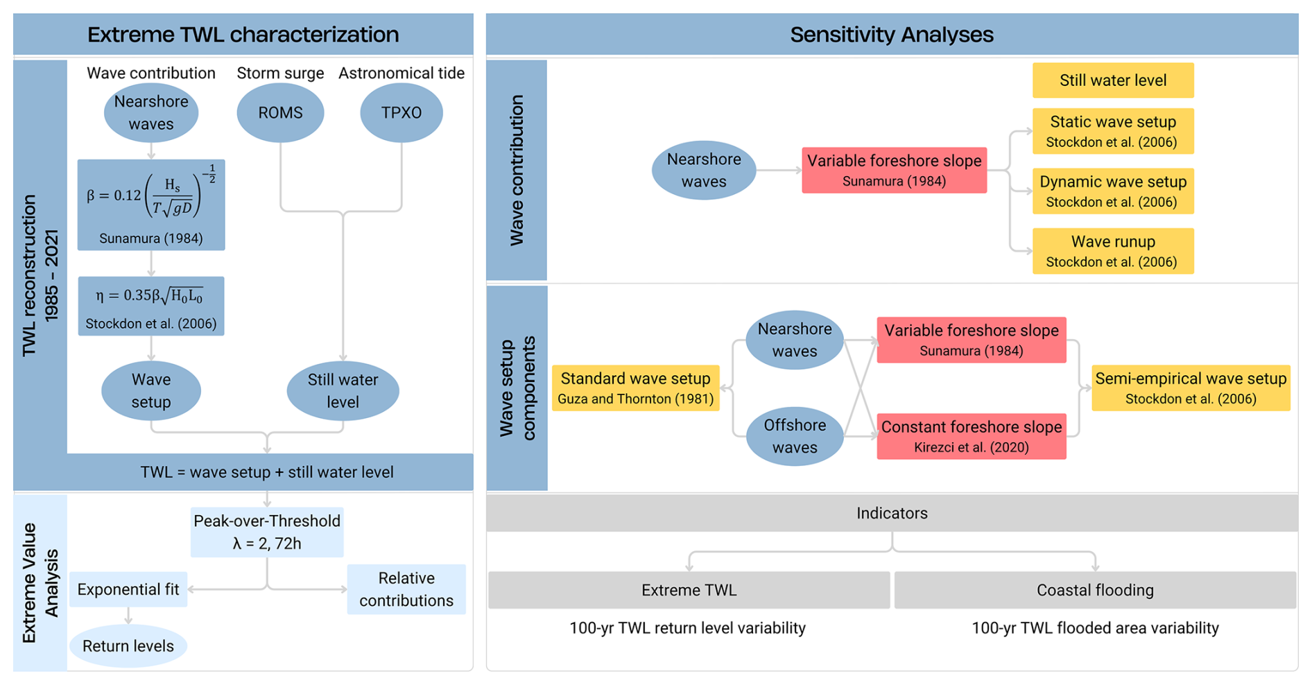
Figure 1 Methodology applied in the present study for TWL hindcast reconstruction and extreme value analysis (left). Sensitivity analyses applied to the wave contribution and wave setup components (right).

2.1 Study Area

The study area comprises the European coastline. Prior to reconstructing the TWL hindcast, coastal target points (CTP) were defined along the European coast with the objective of creating a continuous line of equally spaced points as close to the coast as possible. Due to the lack of high-resolution homogeneous bathymetry data at this scale, the CTPs were selected based on their relative depth ($h/L$, where h represents the water depth and L the corresponding wavelength of the wave peak period with an exceedance probability of 0.1). In total, 51 010 CTP with relative depth of approximately 0.1 were chosen, with an interval of 1 km between them and as close as possible to the coast. These points were used for downscaling wave conditions and reconstructing the TWL.

2.2 Climate-related Datasets

The still water level includes the mean sea level, astronomical tide, and storm surge. Here, the local mean sea level is used as benchmark. The hourly time series of the astronomical tide and storm surge were reconstructed from the tidal constituents of the TPXO9 model (Egbert and Erofeeva, 2002) and from a European regional storm surge hindcast developed using the ROMs model (Shchepetkin and McWilliams, 2005), respectively. The astronomical tide provides data in coastal areas at a spatial resolution of $\mathrm{1}/\mathrm{30}$° (approximately 3.5 km), whilst the European storm surge hindcast used provides storm surge information along the European coast at 5–11 km spatial resolution. The offshore waves were obtained from a European regional hindcast developed with the WaveWatchIII numerical model (WW3; Tolman, 2009). This provides wave outputs along the European coastline at a spatial resolution of $\mathrm{1}/\mathrm{8}$° (10–15 km). The nearshore wave dataset was developed based on the DOW approach (Camus et al., 2013), which combines numerical wave simulations using the SWAN model with advanced statistical techniques in order to reach 1 km spatial resolution throughout the European coastline. Atmospheric forcings from the ERA5 reanalysis (Hersbach et al., 2020) were used to generate these datasets consistently. A more detailed description of the models and their configuration used, as well as an assessment of the data quality in coastal areas by comparison against coastal buoys and tide gauge records is provided in the “Sea level and wave datasets” section of the Supplement and in IHCantabria (2024).

At each CTP, hourly time series were obtained for the astronomical tide, storm surge, offshore wave conditions, and nearshore wave conditions. While nearshore wave conditions were downscaled directly at each CTP, the offshore wave hindcast, storm surge hindcast, and TPXO databases do not share the same spatial resolution. To address this mismatch, data from the nearest grid point was assigned to each CTP for those variables. A sensitivity analysis confirmed the robustness of the node selection method from the marine dynamics databases (see Fig. S6 in the Supplement).

2.3 Total Water Level

The TWL time series was reconstructed from 1985 to 2021 on an hourly basis at each CTP by linearly adding the time series of astronomical tide, storm surge, and wave setup, following Eq. (1).

$$\begin{array}{}\text{(1)}& \mathrm{TWL}=\text{wave\hspace{0.17em}\hspace{0.17em}setup}+\mathrm{SS}+\mathrm{AT}\end{array}$$

where SS is the storm surge and AT the astronomical tide.

Wave setup was used to represent the wave contribution to TWL. Using nearshore wave conditions, it was calculated with the semi-empirical formulation, using Eqs. (2) and (3) (Stockdon et al., 2006) with a variable intertidal slope as given in Eq. (4) (Sunamura, 1984).

$$\begin{array}{}\text{(2)}& {\displaystyle }\mathit{\eta }=\mathrm{0.35}\mathit{\beta }\sqrt{H_{\mathrm{s}}{L}_{\mathrm{0}}}\text{(3)}& {\displaystyle }{L}_{\mathrm{0}}={\displaystyle \frac{g{T}^{\mathrm{2}}}{\mathrm{2}\mathit{\pi }}}\end{array}$$

where β is the foreshore slope of the beach, between the low and high tide limits, H_s is the significant wave height, L₀ is the deep-water wavelength, and T is the wave period.

$$\begin{array}{}\text{(4)}& \mathit{\beta }=\mathrm{0.12}{\left({\displaystyle \frac{H_{\mathrm{s}}}{T\sqrt{gD}}}\right)}^{-\frac{\mathrm{1}}{\mathrm{2}}}\end{array}$$

where g is gravitational acceleration and D is the mean sediment grain size, set at 250 µm, representative of fine to medium grain size and following Rueda et al. (2017). The calculated foreshore slope time series for each CTP was capped at 0.20 and normalized to ensure a mean close to 0.04, reflecting the global median beach slopes based on locally reported values (Barboza and Defeo, 2015). The approach used to apply the foreshore slope approximation followed Melet et al. (2020) and has been validated (see Fig. S7).

Upon the TWL reconstruction, the stationarity of the time series was verified in each CTP and a validation of the hindcast was performed by identifying historical coastal storms observed in the literature and comparing to the values estimated here. In total, 36 events were validated across distinct areas of the European coastline. A summary of the references and locations validated is presented in the Supplement (Table S4). The validation was performed against still water level, static wave setup-based TWL, dynamic wave setup-based TWL, and wave runup-based TWL, following Stockdon et al. (2006).

Since the European coastline reaches high latitudes, the presence of sea ice may affect the impact of the different coastal dynamics considered in this study (e.g., in the Baltic Sea). As all atmospheric-driven dynamics originate from a common forcing, ERA5, the sea ice cover provided by this reanalysis was used to account for the presence or absence of ice. This variable represents the fraction of each grid cell covered by ice. The temporal evolution of ice cover was extracted at the nodes closest to the coastal points. Ice presence was assumed when the coverage exceeded a fraction of 0.5, following the simple ice-blocking scheme used in wave propagation models such as WW3 (e.g., Kumar et al., 2025). Accordingly, when ice was present, the corresponding data at CTPs were excluded from the analysis, as neither waves nor tides effectively reach the coast under such conditions.

2.4 Model Validation Summary

The modeling chain used to reconstruct TWL combines independent, state-of-the-art datasets for tides, storm surges, and waves, each of which was validated against available observations prior to their integration. Table 1 presents a summary of the validation results. Astronomical tides derived from TPXO9v5 were validated against 48 tide-gauge records distributed along the European coastline, showing high skill in reproducing tidal amplitudes and phases, with root mean square errors typically below 10 cm, biases close to zero, and Pearson correlation coefficients exceeding 0.9 at most locations (Table S1, Fig. S1). The storm surge hindcast generated with ROMS was validated against non-tidal residuals from the same tide-gauge network, yielding RMSE values generally between 6 and 15 cm, low bias, and correlation coefficients above 0.7 across most stations (Table S2, Fig. S2).

Table 1 Model validation summary obtained from the different validation analyses performed for the different databases composing TWL, including the foreshore slope.

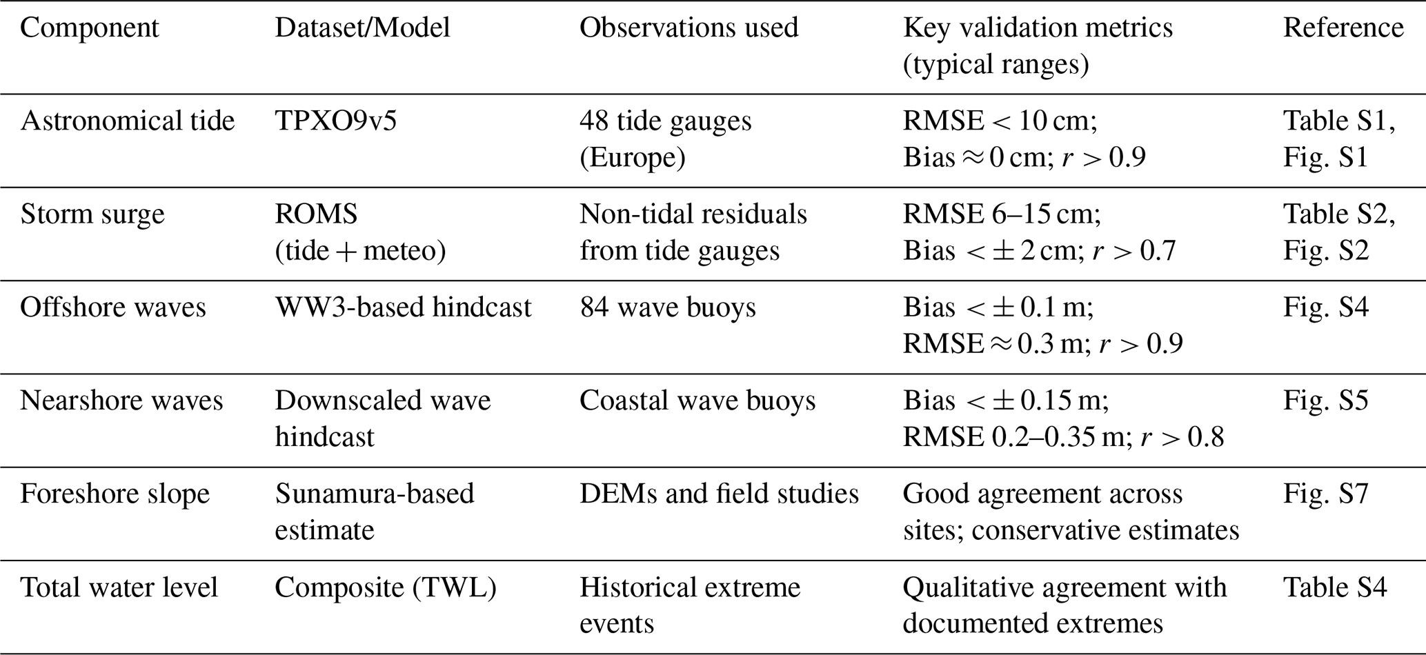
Offshore and nearshore wave hindcasts were validated against buoy observations, showing average biases below ± 0.15 m, RMSE values typically below 0.35 m, and correlation coefficients exceeding 0.8 for the majority of stations (Figs. S4 and S5). The foreshore slope estimation used to parameterize wave setup was independently validated against high-resolution topo-bathymetric data and field-based observations across representative European coastal settings, confirming its suitability for large-scale applications (Fig. S7). The slope validation is intended solely as a consistency check against local estimates rather than a full site-specific calibration.

Direct validation of TWL as a composite variable remains challenging at continental scale due to the scarcity of observations capturing wave-induced water-level contributions. Consistent with previous large-scale studies, TWL reliability is therefore assessed through the validation of its individual components and by comparison with documented historical extreme events. This approach provides confidence that the reconstructed TWL hindcast is robust and appropriate for the large-scale flood hazard analyses targeted in this study.

2.5 Extreme Value Analysis

The POT method was used to identify extreme events in the TWL hindcast. At each CTP, we selected a threshold that resulted in an average of two events per year (λ=2), with a minimum interval of 72 h between events. Next, we estimated the TWL return values (i.e., TWL values associated with return periods) by fitting the extreme sample to an exponential model.

To refine the methodology, we conducted several tests regarding the extreme event selection method, the threshold applied, and the distribution fits. Preliminary tests were carried out on a set of points selected using clustering methods (Camus et al., 2011), as detailed in the Supplement (Fig. S8). We compared the results of return levels and confidence intervals obtained from the AM method using GEV and Gumbel distributions, and from the POT method using both exponential and GPD fits (Fig. S11), as well as different thresholds options tested in POT (Fig. S12). A stability check of the resulting parameters was assessed through a residual life plot (Coles, 2001; Liu et al., 2023) (Fig. S13) and concluded that the optimal average amount of events per year (λ) was two.

At the European scale, we conducted sensitivity analyses on the distribution fits, POT threshold, and POT declustering interval time to ensure the selection of independent events. Regarding the distribution fits, around 13 % of the coast exhibited a significant shape parameter, justifying the use of GPD instead of an exponential distribution (see Fig. S14). Most of these points presented a negative shape parameter and half of them were located in tide-dominated areas, where the TWL is modulated by the astronomical tide. However, due to the narrow confidence bands in these regions, we opted to retain the exponential fit, simplifying the method for continental-scale applications. Additionally, only 6.5 % of the coast rejected the Anderson–Darling null-hypothesis which would justify the use of GPD (see Fig. S15). Regarding the POT threshold, λ=2 represented a reasonable balance between accuracy, robustness, and sample size to be used in EVA (see Fig. S9, sensitivity analysis on POT threshold). Regarding the declustering interval, a 72 h minimum interval resulted in the largest amount of CTP significantly fitting an exponential fit (93.5 %), according to the Anderson–Darling test, compared to 48 and 96 h intervals (see Fig. S10, sensitivity analysis on POT interval).

2.6 Relative Contributions of TWL components

To better understand the dominant conditions at each CTP, the relative contributions of each TWL component were computed (astronomical tide, storm surge, and wave setup). The contribution of each component was calculated by extracting its value from its respective time series and determining its proportion relative to the TWL at the corresponding time step. For mean conditions, we calculated this for each time step within the entire time series and then calculated the mean contribution for each component. For extreme conditions, relative contributions of each TWL component were calculated for each exceedance peak identified by POT.

2.7 Sensitivity Analyses

Figure 1 also presents the sensitivity analyses performed regarding the inclusion of waves in this study. Within these analyses, the same EVA method (POT with a threshold of λ=2 fitted to an exponential fit) was adopted in all cases. Two indicators were used to determine how sensitive results are to the different options tested in each analysis. On the one hand, the 100 year TWL was analyzed. The variability of results was studied to determine the relative influence each option has on the outcome. On the other hand, the corresponding 100 year TWL flooded area (FA) resulting from a static flood model applied to the European floodplain was evaluated. The flood model applied was a simple GIS-based bathtub approach, in which any area below a certain water level is considered flooded, provided it is hydraulically connected to the sea. This method was only used as a first-order approximation of the flooded area for comparative purposes in the sensitivity analyses. The floodplain was defined as the terrain below 15 m of elevation and hydraulically connected to the sea, based on the 25 m resolution Copernicus EU-DEM (Copernicus, 2019). Additional sensitivity analyses performed on TWL resolution and EVA (i.e., POT threshold and POT declustering interval) are presented in the Supplement.

2.7.1 Sensitivity analysis: wave contribution

As part of the validation of the TWL reconstruction, different options were tested in terms of the characterization of the wave contribution. Following the equations by Stockdon et al. (2006) with a variable intertidal slope as given in E. (4) (Sunamura, 1984), we tested: (i) static wave setup, following Eq. (2); (ii) dynamic wave setup, according to Eqs. (5) and (6); and (iii) wave runup, from Eq. (7). After each wave contribution was computed, the corresponding TWL was reconstructed by adding the storm surge and astronomical tide time series. The same resulting TWL variants used in this analysis, were the ones adopted in the TWL reconstruction validation.

$$\begin{array}{}\text{(5)}& {\displaystyle }{S}_{\text{IG}}=\mathrm{0.06}\sqrt{H_{\mathrm{s}}{L}_{\mathrm{0}}}\text{(6)}& {\displaystyle }{\mathit{\eta }}_{\text{dyn}}=\mathit{\eta }+S_{\text{IG}}\text{(7)}& {\displaystyle }{R}_{\mathrm{2}}=\mathrm{1.1}\left(\mathit{\eta }+{\displaystyle \frac{\sqrt{H_{\mathrm{s}}{L}_{\mathrm{0}}(\mathrm{0.563}\mathit{\beta }+\mathrm{0.004})}}{\mathrm{2}}}\right)\end{array}$$

2.7.2 Sensitivity analysis: wave setup components

Three elements were tested in the wave setup analysis: (i) the wave dataset (downscaled nearshore wave conditions and large-scale wave conditions, hereafter referred to as offshore wave conditions); (ii) the foreshore slope approximation (variable and constant); and (iii) the wave setup formulation (semi-empirical and standard). The combinations of these elements resulted in 6 TWL reconstruction approaches.

First, we calculated wave setup with the same semi-empirical formulation (Eq. 2) but applying offshore wave conditions instead of nearshore downscaled conditions. Then, we applied the wave setup formulation by Guza and Thornton (1981) to both offshore and nearshore wave conditions, following (Eq. 8).

$$\begin{array}{}\text{(8)}& \mathit{\eta }=\mathrm{0.2}{H}_{\mathrm{s}}\end{array}$$

Table 2 Approaches used to reconstruct TWL in the sensitivity analysis of wave setup components, showing their respective combinations of wave datasets, foreshore slope approximations, and wave setup formulations adopted.

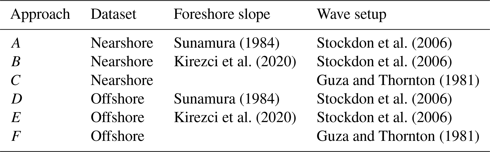
For the comparison of foreshore slope approximations, we applied variable slopes (Sunamura, 1984) to offshore wave conditions and also adopted a constant foreshore slope of 0.03 (Kirezci et al., 2020). Both foreshore slope options were used in conjunction with the semi-empirical wave setup formulation shown in Eq. (2) (Stockdon et al., 2006) and with both wave datasets. In total, 6 approaches were tested, as shown in Table 2. While approach A represents the methodology proposed in the present study, the remaining approaches were only used in this sensitivity analysis.

3 Results

3.1 Wave and sea level datasets processing and total water level computation

Figure 2 presents the 2021 hindcast of all variables used in this study for four coastal target points (CTP) in which we reconstructed the TWL. The CTPs used as examples throughout this study were selected from a list of test points selected with a K-means clustering technique applied to the relative contributions of the TWL components (see Fig. S8). Point 1 is located on the Atlantic coast of France, point 2 in Estonia in the Baltic Sea, point 3 in Greece in the Mediterranean Sea, and point 4 in Norway (Fig. 2g). These points represent the centroids of the four most distinct K-means clusters. Offshore wave conditions (Fig. 2a) were downscaled to the coast (hereinafter, nearshore wave conditions; see Fig. 2b), from which wave setup (Fig. 2c) was calculated to represent the wave component. Storm surge (Fig. 2d) and astronomical tide data from TPXO (Fig. 2e) were then added to the wave setup hindcast to obtain the TWL (Fig. 2f) time series. As a consequence, the variability of the TWL reflects the heterogeneity of the spatial distribution of its three components. The distinction between offshore and nearshore wave conditions is evident, particularly at points 3 and 4 where notable differences are observed. The results highlight that while the TWL time series of points 1 and 4 are primarily influenced by tides, point 2 appears to be dominated by storm surge. However, although point 4 shows smaller oscillations, higher wave setup values raise its TWL time series, unlike point 1, where the series remains centered around 0 m.

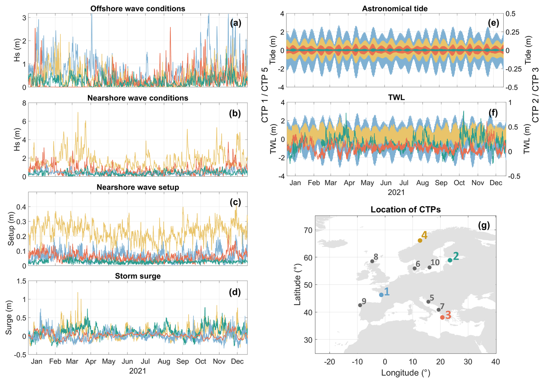
Figure 2 Hindcast time series referred to 2021 for the following variables: (a) offshore significant wave height, (b) nearshore significant wave height, (c) nearshore wave setup, (d) storm surge, (e) astronomical tide, and (f) TWL. (g) Location of the CTPs used as examples. Time series are represented in the same colors as the corresponding CTP. Gray CTPs represent the remaining 6 test points selected with K-means. Note. Left axis in (e) and (f) refer to CTPs 1 and 4, right axis to CTPs 2 and 3.

3.2 Validation of TWL reconstruction

Figure 3 presents the validation of the TWL hindcast. The validation was performed by comparing our estimated values against previously observed historical storms across the study area, based on previous studies. For more details on the references used in the validation of the TWL, please refer to the Supplement (Table S4). In total, four TWL approaches were tested: still water level (SWL; astronomical tide and storm surge) (Fig. 3a), SWL combined with static wave setup (Fig. 3b), SWL with dynamic wave setup (Fig. 3c), and SWL with wave runup (Fig. 3d).Within the options tested for a standardized TWL reconstruction approach at the large-scale, the TWL based on SWL combined with static wave setup shows the best performance with 87.9 % of the TWL variability being captured, an RMSE of 0.438 m indicating an average error of 7.5 %, and a bias of −0.151 m. Meanwhile, TWL based solely on still water level leads to a greater level of underestimation and the remaining two approaches, an even greater level of overestimation. These results highlight the importance that other aspects might have on the resulting TWL and, consequently, coastal flooding. Notably, the cases in which static wave setup-based TWL underestimates TWL the most are located along the Atlantic coast, such as Santander (Spain), Brouage (France), and the Elbe Estuary (Germany). This could be an indication that these regions are sensitive to infragravity waves since dynamic wave setup-based values provide more accurate estimates of TWL.

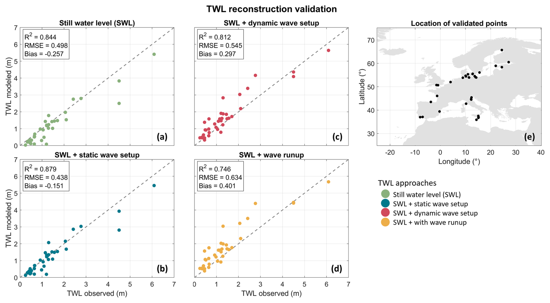
Figure 3 TWL reconstruction validation based on TWL with (a) still water level, (b) static wave setup, (c) dynamic wave setup, and (d) wave runup when comparing historical coastal storms observed in different points across the study area, according to previous studies. (e) Location of validated points.

3.3 Extreme value analysis of the total water level

Figure 4 shows the TWL threshold used in the POT method to select the extreme events (Fig. 4a) as well as the corresponding TWL percentiles associated with these thresholds for each CTP (Fig. 4b). The results emphasize the importance of considering the spatial variability of thresholds as neither the TWL thresholds nor the corresponding percentiles are uniform across the study area. When adopting λ=2, the TWL threshold ranges from 0.3 m in the Messina Strait (Italy) to 7.2 m in the Bristol Channel (Great Britain), while corresponding percentiles range from P99.2 south of Stockholm (Sweden) to P99.9 in the Wash (Great Britain). The entire study area is characterized by percentiles above P99, with 97.3 % of the CTPs displaying a percentile above P99.5. When applying a constant percentile threshold across the study area, λ varies from 12.1 to 68.3 for P90 and 1.4 to 14.5 for P99.5 (see Fig. S16). This suggests that using a constant threshold would lead to an excessive number of events in regions such as the Dutch coast and the Irish Sea, for example. Whereas in others regions, such as the Baltic Sea, the sample size would be insufficient, resulting in unstable results of EVA and return levels of TWL.

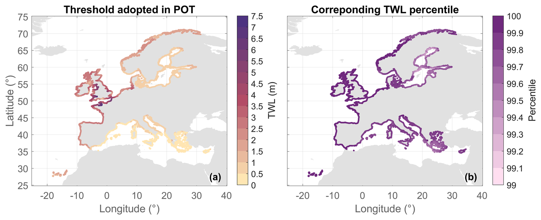
Figure 4 (a) Spatial distribution of the TWL threshold adopted in POT in each CTP. (b) TWL percentile that corresponds to the threshold adopted in each point.

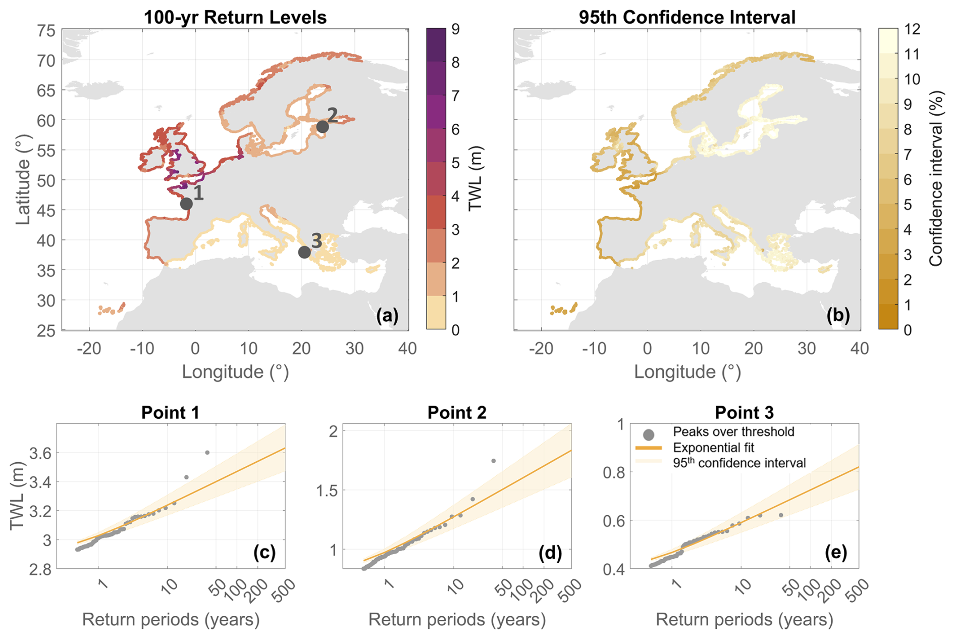
Figure 5 (a) Spatial distribution of the 100 year return period TWL resulting from POT with an exponential fit. (b) Spatial distribution of the 95th confidence interval relative to the 100 year TWL event, in percentage. (c–e) Examples of individual CTPs with the exponential fits applied to the POT samples to extract return levels of TWL.

Figure 5 provides the spatial distribution of the 100 year TWL for the coast of Europe and the associated 95th confidence interval values at each CTP (Fig. 5b). This result is shown in percentage relative to the return level itself to facilitate the comparison of the results between different regions. For example, the 100 year TWL in France is 3.5 ± 0.12 m, or 0.3 % (Fig. 5c). While in Estonia it is 1.6 ± 0.17 m, or 10.8 % (Fig. 5d) and in Greece, it is 0.7 ± 0.07 m, or 9.8 % (Fig. 5e). Higher confidence interval values indicate a broader confidence band and, consequently, greater uncertainty in the distribution fit. With TWL values reaching up to 8.5 m in the Bristol Channel, the highest 100 year TWL values are observed around the British Isles and along the English Channel. This region also shows the narrowest confidence intervals, with the confidence band fluctuating by less than 4 % for the 100 year TWL. This may be linked to the dominant tidal regime in this area, which due to its high amplitude modulates both mean and extreme conditions. The Mediterranean Sea shows the lowest 100 year TWLs, with values ranging from 0.49 m in the Messina Strait to 2 m in the Adriatic Sea. In this region, the 95th confidence interval increases from approximately 6.5 % in the Gibraltar Strait to 11 % in Greece. In the Baltic Sea, 100 year TWL range from 0.91 m south of Stockholm to 2.52 m in St. Petersburg, increasing towards the regions of the inner gulfs. Additionally, this region displays the widest confidence intervals, ranging from 9 % to 12 % for the 100 year TWL. Overall, the results suggest that return level estimates are more reliable in areas where TWL is dominated by the astronomical tide, such as the Bay of Biscay, where confidence intervals range from 2 % to 5 %. Similar behavior, albeit with slightly lower values, is observed for the 50 year TWL (see Fig. S17).

3.4 Relative contributions of mean and extreme total water levels

Figure 6 displays the average storm conditions based on the relative contribution of TWL components at peak moment. Examples are shown for three points: point 1 on the Atlantic coast of France (Fig. 6a), point 2 in Estonia in the Baltic Sea (Fig. 6b), and point 3 in Greece in the Mediterranean Sea (Fig. 6c). The shape of the average storm at each point reflects the dominant TWL component during storms. We observe distinct behaviors: point 1 is tide-dominated, point 2 is storm surge-dominated, and point 3 reflects mixed-storm conditions. While point 1 shows semi-diurnal tidal oscillations, point 2 exhibits a single TWL peak, characteristic of a typical storm surge event. Point 3 shows a similar pattern to point 2, but also includes tidal noise throughout the average event.

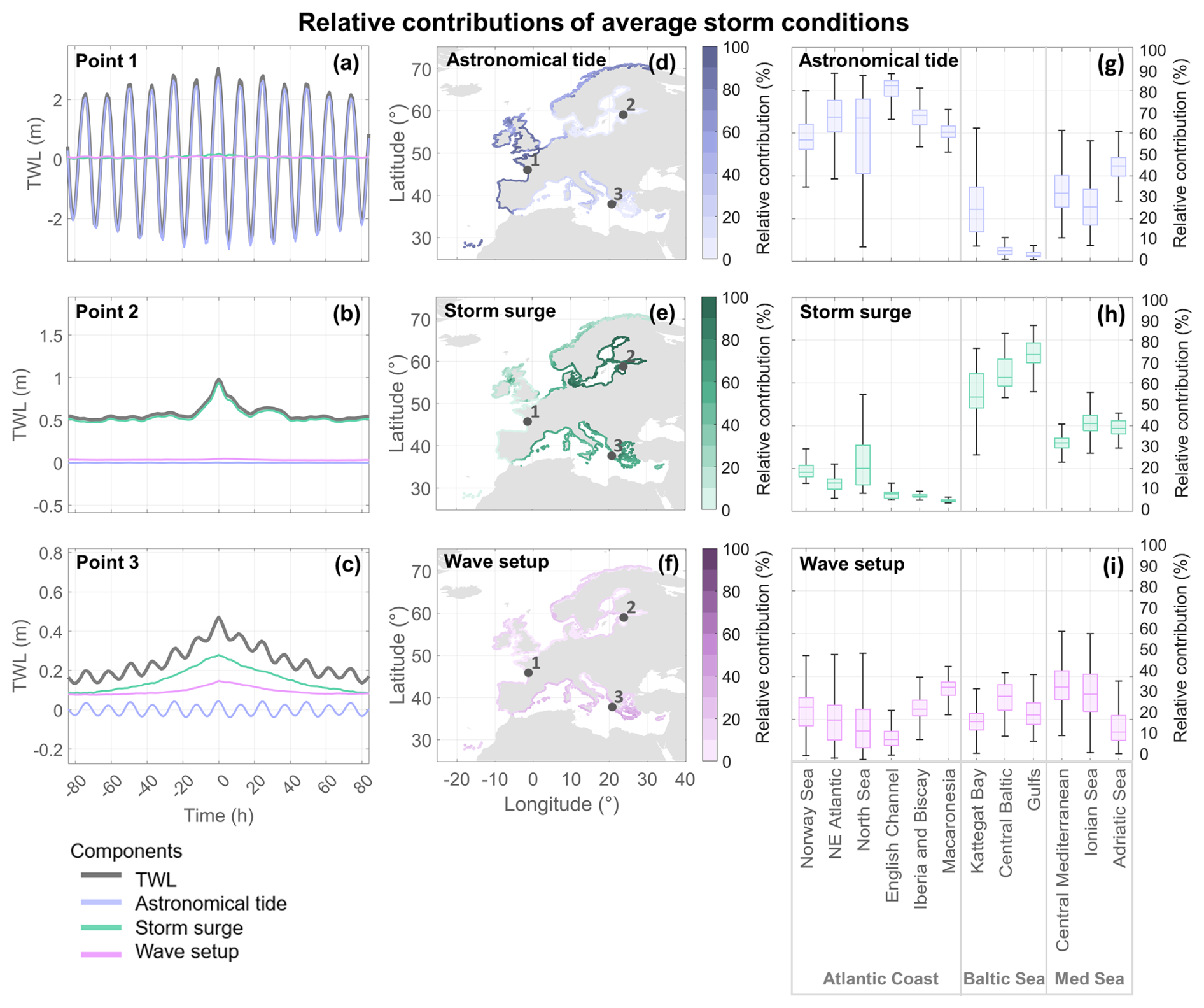
Figure 6 (a–c) Examples of individual CTPs with average storm conditions per TWL component. Spatial distribution of mean relative contributions of (d) astronomical tide, (e) storm surge, and (f) wave setup under extreme conditions. (g–i) Dispersion of relative contributions of TWL components per European basin, grouped per European region.

The spatial distribution of TWL components' relative contributions is presented in Fig. 6d–f. Although diverse, it is possible to observe patterns across the study area and the larger European regions previously identified in the study: Atlantic coast, Baltic Sea, and Mediterranean Sea. Figure 6 also presents the dispersion of relative contributions of TWL components, aggregated per European basin. These plots support the graphical representation of the different patterns observed and the characterization of the three macro-regions (Fig. 6g–i).

First, the dominance of the astronomical tide along the Atlantic coast is evident and modulates storms regardless of their origin, although at different levels depending on the basin. Tidal contributions along the most exposed Atlantic coast can reach 100 %, especially along the Atlantic Iberia and Bay of Biscay. The more northern basins tend to present less dominance of the astronomical tide and more presence of storm surge and wave setup. Notably, the North Sea is the most balanced basin in this region in terms of the contributions of the three components. This is likely due to its shallow waters and extensive continental platform which enhance the action of storm surge. Second, the highest storm surge contributions found in the Baltic Sea also reach 100 %. Storm surge tends to be higher in the Baltic Sea due to its wider continental platform. The transition role of the Kattegat Bay is reflected in the higher contribution of astronomical tide as opposed to the remaining two basins. Third, although the highest wave setup contributions are in the Mediterranean Sea, this region also experiences storm surge contributions above 50 %. Within this region, the Adriatic Sea shows the highest contribution of storm surge likely because of its shallow water enabling the propagation of storm surges as well as its lower level of exposure to incoming waves. Meanwhile, the Ionian Sea presents the highest contributions of wave setup, likely because of its exposure levels and lower astronomical tide when compared to the Central Mediterranean basin.

3.5 Sensitivity analysis: wave contribution component

Figure 7a presents the variability of the 100 year TWL based on different options of the wave contribution component: still water level (SWL), SWL combined with static wave setup, SWL with dynamic wave setup, and SWL with wave runup. The highest levels of variability are observed in the Mediterranean Sea, more specifically in Central Mediterranean and Ionian Sea, which could be an indication of relatively larger contributions of waves to TWL compared to the remaining two components, or a response to low ranges of TWL, indicating that even a slight change in the wave contribution is reflected in the estimation of TWL extremes. Meanwhile, the lowest variabilities are found in the Baltic Sea, probably a response to its limited exposure to incoming waves.

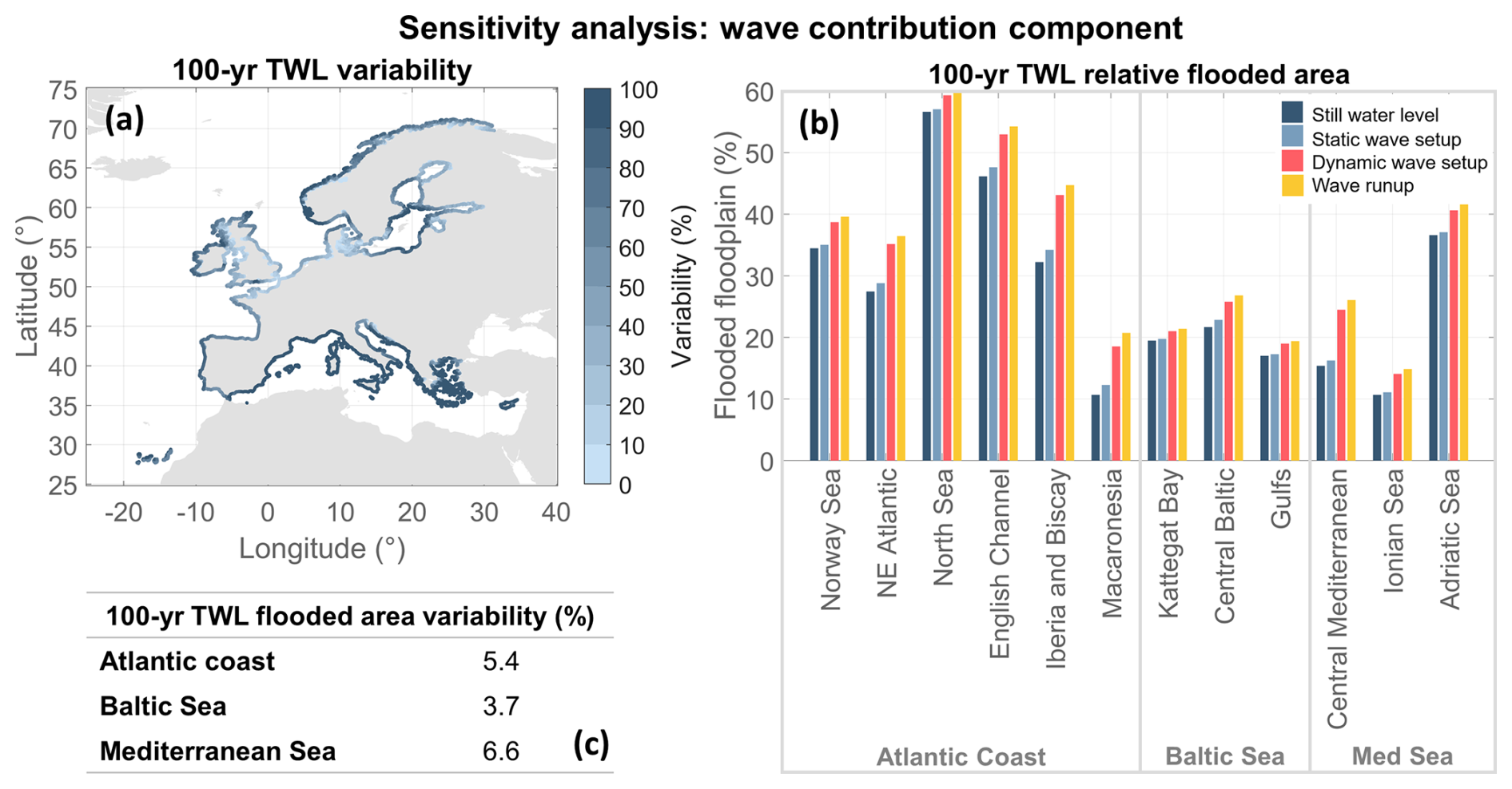
Figure 7 Sensitivity analysis of the wave contribution considered in the TWL reconstruction: still water level (SWL) vs. SWL combined with static wave setup vs. SWL with dynamic wave setup vs. SWL with wave runup. (a) 100 year TWL variability found in the results. (b) Results of flooded area proportional to the floodplain in each European basin considering the 100 year TWL. (c) Variability of 100 year TWL flooded area per European region.

Figure 7b presents the FA per European basin, relative to their respective floodplain area, under the 100 year TWL when adopting different wave contribution components. Overall, the highest increase in the FA occurs when changing from a static wave setup based-TWL to a dynamic wave setup based-TWL. The basins most affected include Central Mediterranean and Iberia and Biscay. The former is located in a region typically known for coastal wave storms (Lobeto et al., 2024), while the latter appears to be a region sensitive to infragravity waves, previously observed in the TWL reconstruction validation as well. Meanwhile, the least affected basins are Kattegat Bay and the Gulfs, both located in the Baltic Sea. Besides presenting low values of TWL, these basins are also amongst the steepest floodplains. When looking at the macro EU regions, the most affected one is the Mediterranean Sea, followed by the Atlantic coast and the Baltic Sea (Fig. 7c). These results highlight a clear spatial variability of the wave contribution to TWL. Finally, the European FA with SWL is 36.09 % of the overall floodplain area. Including static wave setup increases the relative FA increases to 36.82 %, dynamic wave setup to 40.40 %, and wave runup to 41.23 %. These results show that while the large-scale results do not change dramatically, it is important to zoom in to smaller regions and basins to identify areas in which such decisions might have the greatest impact.

3.6 Sensitivity analysis: wave setup components

Figure 8 presents the sensitivity analysis of the different TWL approaches tested based on wave setup components. Figure 8a compares the 100 year TWL under offshore versus nearshore wave conditions. Positive values indicate that offshore wave-based TWL is higher than nearshore wave-based TWL, and negative values indicate the opposite. The results highlight the spatial variability of the TWL outcomes. Generally, offshore data results in lower TWL along the Atlantic coast and higher TWL in the Baltic and Mediterranean Seas compared to nearshore data. This suggests a greater degree of wave transformation on the Atlantic coast than in the semi-enclosed seas.

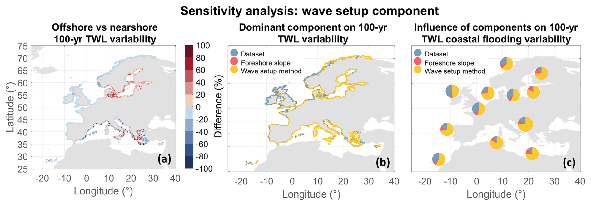
Figure 8 Sensitivity analysis of the wave setup components: data resolution, foreshore slope approximation, and wave setup formulation. (a) Differences in 100 year TWL when applying offshore instead of nearshore wave conditions. This plot isolates the influence of wave data resolution by comparing TWL approach D against A as presented in Table 2. (b) Dominant component explaining the 100 year TWL variability. (c) Influence of wave setup components on the 100 year flooded area variability averaged per EU basin.

Figure 8b identifies the most influential wave setup component when comparing different TWL modeling approaches. Using the 100 year TWL as an indicator, 29 % of CTPs are most sensitive to dataset selection, while 0.1 % are most influenced by the foreshore slope approximation and 70.9 % are most influenced by the wave setup method. Dataset selection is the dominant factor along the Atlantic coast. In contrast, the wave setup formulation becomes more important in the Baltic and Mediterranean Seas. Semi-enclosed seas exhibit lower TWLs making the accuracy of wave setup estimation crucial. Even the smallest errors in this component can lead to significant discrepancies in the TWL predictions, potentially affecting the accuracy of coastal impacts assessments. Additionally, the low influence of the foreshore slope approximation may be due to the conservative approach adopted for capping and normalizing the foreshore slopes (Melet et al., 2020).

Figure 8c presents the influence that each wave setup component tested has on the resulting 100 year TWL FA, averaged per European basin. Across the entire study area, the most influential element is the wave setup formulation with values ranging from 49.3 % along the NE Atlantic basin to 84.0 % in the Central Baltic Sea. When comparing the dataset and the slope approximation components, the Baltic Sea presents more influence from the slope approach, with the exception of the Kattegat Bay which could be described as a transition region rather than being part of the Baltic Sea. Moreover, Central Mediterranean also presents higher influence of the slope approximation than the dataset. The difference, however, is only 0.2 %. The remaining basins across the study area, show the slope approach as the least influential element. When comparing the influences of the dataset and the wave setup formulation, most of the study area present a negative correlation. Along the Atlantic coast and the Baltic Sea, as the influence of the dataset increases, the influence of the wave setup formulation decreases.

3.7 Uncertainty in extreme values of TWL

Table 3 presents the overall characterization of the study area regarding TWL extremes, aggregated per EU basin, including the overall uncertainties of 100 year TWL and its corresponding FA. When looking at the entire study area, 100 year TWL has an uncertainty of 24.8 %. As more detail is added to the analysis, the 100 year TWL uncertainty decreases to 17.0 % along the Atlantic coast and 15.8 % in the Baltic Sea, while it increases to 39.9 % in the Mediterranean Sea. In most cases, 100 year TWL uncertainty increases with increasing relative contribution of wave setup. Notably, the European basins with the highest relative contributions of wave setup, Central Mediterranean and Ionian Sea, are also the ones with the highest uncertainties of the 100 year TWL. Meanwhile, the basins with the lowest relative contributions of wave setup (English Channel and Kattegat Bay) are also the ones with the lowest 100 year TWL uncertainty. Even though this result is likely a reflection of the focus given to the wave contribution to TWL, it points to the role waves partake on TWL uncertainty.

Table 3 Characterization of the study area based on TWL extremes and aggregated per EU basin, region, and the entire study area. EVA results are summarized as TWL threshold corresponding to a λ=2 and 100 year TWL (mean ±standard deviation), following the proposed methodology. Relative contributions refer to average per basin and considering all peaks identified by POT. Uncertainty quantification considers all sensitivity analyses performed, including the ones presented in the Supplement (i.e., wave contribution, wave setup elements, TWL resolution, POT threshold, and POT minimum interval).

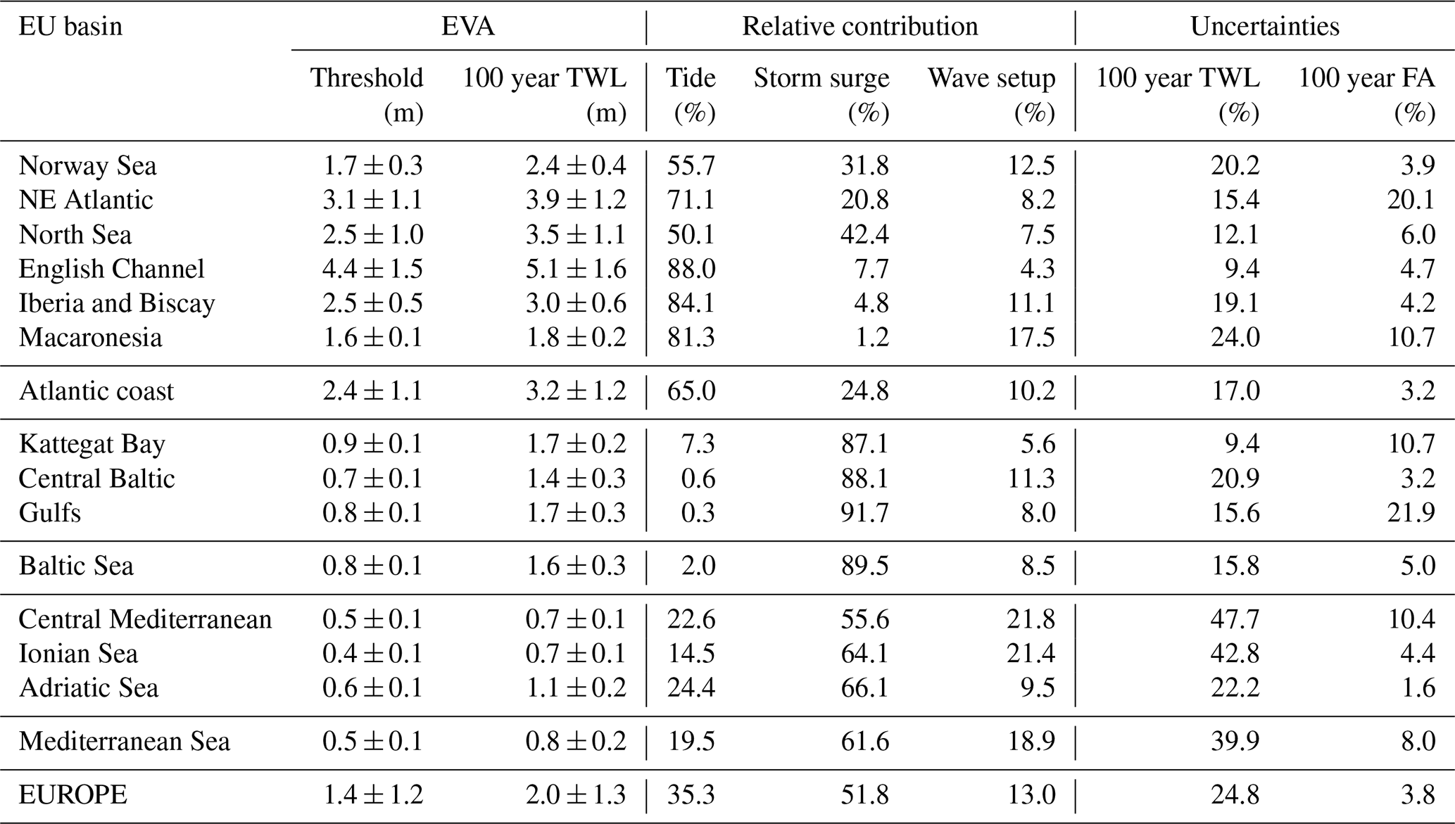
Regarding the 100 year FA, the study area presents an uncertainty of 3.8 % which decreases to 3.2 % along the Atlantic coast and increases to 5.0 % and 8.0 % in the Baltic and Mediterranean Seas, respectively. This does not mean that the European scale map is more reliable but perhaps that it is masking some key responses coastal impacts might have when a different wave contribution is adopted, for example. Overall, uncertainties in 100 year TWL and FA do not necessarily correlate. The results show that large uncertainties in 100 year TWL, when occurring in areas where TWL is typically low, may lead to minimal variability in FA. This is because the variations in 100 year TWL remain small compared to changes in terrain elevation, limiting their impact on flood extent.

3.8 Classification of extreme TWL events

Figure 9 presents the European classification of extreme TWL events, considering the 100 year TWL and the dominance of TWL components regarding their relative contributions. The results show that there are no regions where the wave setup dominates, although it could be an important driver of extreme events in addition to a relevant source of uncertainty. The highest 100 year TWLs are found in areas where the astronomical tide dominates, mainly along the Atlantic coast. In the Baltic Sea, storm surge dominates all CTPs analyzed and the most sheltered areas are where the 100 year TWL are the highest. In the Mediterranean Sea, the most exposed regions are where extreme events are mostly mixed, probably indicative of the wave setup contribution which might not be enough to dominate but still relevant in decreasing the influence of the other TWL components.

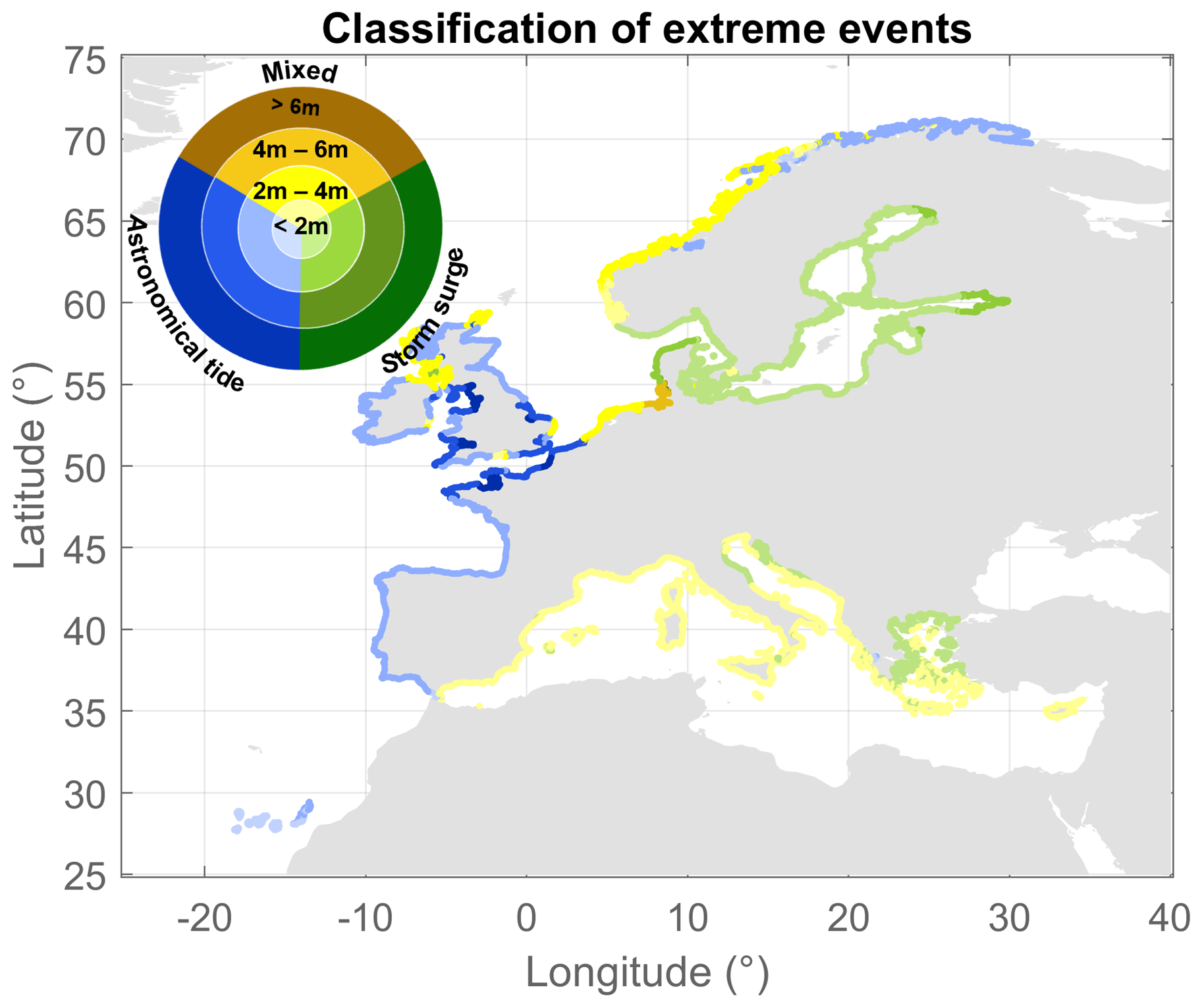
Figure 9 European classification of extreme events considering the range of 100 year TWL and the dominance of TWL components regarding their relative contributions.

4 Discussion

The large-scale TWL calculation is complex and presents several challenges. We have presented a methodology for estimating large-scale TWL extremes and applied it to the European coast at the highest resolution to date. For the first time, this was done using nearshore wave conditions, particularly important for semi-enclosed European seas, where offshore data can lead to TWL overestimation. The methodology developed addresses the key challenges introduced regarding the inclusion of the wave contribution in the TWL, the TWL reconstruction, and the EVA method selected to characterize extreme events. As a consequence, it also introduces limitations inherited from some of the approaches adopted.

Concerning the wave contribution, even though the use of static wave setup as a component of TWL was validated, we acknowledge that this component may be slightly overestimated in areas such as the Baltic and Mediterranean Seas. Notably, this may also influence the relative contributions of the TWL components. Several factors influence the accuracy of wave contribution estimates. First, we use a semi-empirical setup formulation developed for open-coasts and beaches. It should be noted that although both our results and the literature indicate semi-empirical formulations as more appropriate and representative of current best practice, they also present limitations (Dodet et al., 2019). For example, the formulation adopted here was not designed for use in all types of wave regimes or beach profiles (Plant and Stockdon, 2015). Second, we rely on modeled foreshore slopes with capping and normalization, which may not fully capture the range and distributions of observed beach slopes in different coastal environments. This simplification can lead to the underestimation of the wave contribution in steep slopes or overestimation in gentler ones (Melet et al., 2020). Third, the adoption of a constant sediment grain size in the application of the Sunamura (1984) foreshore slope approximation is a necessary generalization at this scale and cannot fully represent the entire study area. This decision might overestimate the resulting foreshore slopes in areas such as wetlands and mudflats which have finer sediment grain sizes. However, although beach types and sediment materials are diverse across the European continent, the value adopted here follows the global study by Rueda et al. (2017) and agrees with values observed in smaller scale studies across the study area (Anthony and Héquette, 2007; Duo et al., 2020; Egon et al., 2025; Horn and Walton, 2007).

With respect to the TWL reconstruction, the linear approach adopted inevitably simplifies some coastal processes, particularly in areas such as bays and estuaries, for example. Although hydrodynamic modeling would be the ideal method to solve local processes, it is not yet feasible at this scale due to data and computational requirements. Nevertheless, although our TWL reconstruction does not explicitly resolve nonlinear interactions, these are partly accounted for in the underlying databases. For instance, the storm surge database includes nonlinear effects with the astronomical tide and the nearshore wave dataset considers sea level changes due to tide. Moreover, direct validation of reconstructed TWL as a composite variable at the European scale is inherently challenging as it is limited by observational constraints. While SWL can be validated with tide gauges, wave conditions can be validated with buoys. However, the increase in coastal water level as a result of the wave contribution is not captured by wave buoys and tide gauges do not capture wave runup and only partially represent setup effects, while spatially extensive observations of shoreline TWL are not available across Europe. An alternative is to use instruments such as pressure sensors or ADCPs that capture local observations. However, even these are limited by the need for corrections, regular maintenance, and their localized nature. The lack of observational data and instruments enabling direct validation of TWL has led previous studies to validate TWL indirectly, by validating each component individually (e.g., Dalinghaus et al., 2025; Liu et al., 2025; Vousdoukas, et al., 2018a). The evaluation presented here also relies primarily on the quantitative validation of the individual TWL components, including tides, storm surge and nearshore wave conditions, together with consistency checks of the reconstructed TWL during storm events. Therefore, given the successful validation presented for the TPXO, ROMS, offshore wave, and nearshore wave databases as well as the foreshore slope, we consider the TWL hindcast to be robustly validated for the purposes of this study. It should be noted that although the Sunamura-based slope is derived from validated wave forcing and compared against local estimates in selected hotspots, it cannot fully resolve local morphological complexity or the influence of coastal structures at this scale. Sensitivity analyses further indicate that, across most of Europe, uncertainty in slope propagates to TWL though it remains secondary compared to surge and wave contributions at continental-scale.

Furthermore, the TWL validation presented by comparing historical storms identified by previous studies, showed that the extreme events analyzed were well represented by the TWL hindcast, even though most of the observed storms were referenced to tide gauges, which do not capture wave contribution. Given the lack of data to validate TWL, the use of tide gauge information to validate TWL is common practice in the literature (Le Gal et al., 2023; Kirezci et al., 2020; Treu et al., 2024; Wing et al., 2024). Similar to the results found here, when comparing validation results with and without wave contribution, Kirezci et al. (2020) detected more accurate estimates when including wave setup. The authors debate whether this is an underestimation of the SWL or the influence of waves given that these results are even more pronounced under extreme than average conditions. Even though the reasons behind these results remain inconclusive, it is clear that when considering the wave contribution, extreme events are better captured by TWL reconstructions, with the TWL validation serving as a consistency check to assess the representation of TWL during storm events.

Regarding the EVA methodology, its adoption in tide-dominated regions require careful evaluation. Tides are deterministic, periodic, and autocorrelated, which contradicts the EVA assumption of a sample of independent, abnormally extreme events. However, by applying EVA to the TWL composed of both deterministic and stochastic variables, random exceedances emerge due to the interaction of residuals with tides, introducing variability in the extremes. Therefore, fitting an extreme value distribution to the aggregated TWL, as performed in this study, remains a valid and informative approach and allows the tail behavior of the distribution to be characterized even in regions dominated by astronomical tide.

One key outcome is the strong influence that methodological choices concerning the wave contribution to TWL reconstruction have on the results. The European flooded area varies by up to 10 %, depending on the wave contribution, wave dataset selection, foreshore slope approach, and wave setup formulation, with the largest differences arising from the choice of wave setup formulation. Using the Guza and Thornton (1981) method yields 4 %–7 % more flooded area than the Stockdon et al. (2006) formulation, regardless of the foreshore slope assumption, whereas using a constant foreshore slope yields 1 % more flooded area than incorporating variable slopes. Similarly, nearshore TWL produces 3 % more flooded area than offshore TWL. The regional differences in the importance of the three components of wave setup can be explained by the geometry and exposure of the different regions. On the one hand, the steeper bathymetry of the Atlantic coast enhances wave shoaling processes, leading to higher waves as they approach the shore. In contrast, the shallower waters and gentler slopes in the Baltic and Mediterranean Seas tend to result in greater wave energy dissipation, as waves encounter the seabed earlier and lose energy more quickly. Although not accounted for in this study, nonlinear processes involved in wave transformation, such as refraction and wave-breaking mechanisms, could also help explain such differences as wave transformation processes affect TWL mainly in areas with steep beach slopes and complex offshore bathymetry (Serafin et al., 2019). On the other hand, the Atlantic coast has a larger fetch, allowing for the development of higher waves, and it is more exposed to coastal winds, which amplify wave energy. Conversely, the Mediterranean Sea has a smaller fetch, producing more localized and less energetic waves. These factors also result in greater discrepancies in wave conditions within the semi-enclosed seas compared to the Atlantic coast, where offshore and nearshore wave conditions are more similar. While these effects merit further analyses at a higher resolution and on a smaller scale, the results suggest that relying on offshore wave conditions, common in the literature, may lead to an underestimation of the actual flood extent.

Besides the adoption of nearshore wave conditions in the estimation of the wave setup, the 1 km TWL hindcast has an unprecedented spatial resolution for this study area. When working with nearshore (downscaled) wave conditions, higher resolution is preferable to fully exploit the quality of the available information. Nearshore wave conditions capture local-scale variability, and the higher the resolution, the more faithfully the methodology represents these processes, making the best possible use of the data. We emphasize that the objective is not to improve flood extent estimates directly, but to provide physically consistent high-resolution boundary conditions required for next-generation coastal flood models. With 1 km resolution data, the physics of the processes are better captured because we better resolve wave-height gradients, coastline orientation effects, and exposure heterogeneity. This is particularly relevant in complex coastlines (e.g., embayed or headland-dominated), where coarse resolution fails to capture gradients that are resolved at 1 km. A sensitivity analysis of the TWL resolution showed that the reduction in spatial resolution affected the flood extent up to 14 % in some areas (Table S3, sensitivity analysis on TWL resolution). The limited differences in some flooded area comparisons are expected given the DEM resolution and its vertical error, which can mask sensitivity to small changes, revealing differences primarily for larger forcing contrasts. Notably, the basins most sensitive to TWL resolution are located in the Atlantic region likely because of the greater discrepancies between TWL magnitudes and terrain elevations in addition to the increased need for accurate data when modeling a wider range of wave conditions given the highly energetic and variable wave climate in this region (Lobeto et al., 2024).

A second outcome is the application of an EVA methodology that is appropriate for large-scale studies. The POT approach focuses on high-magnitude events, unlike annual maxima (AM) methods, which assume that a single extreme event occurs per year. Our findings show that threshold selection greatly influences sample size, particularly when applying a constant percentile threshold. Comparing to previous studies, we found that 77.1 % of the study area exhibits more than 12 events per year when the threshold of P97 used by Le Gal et al. (2023) is adopted. Meanwhile, if the thresholds of P98 and P98.5 used by Kirezci et al. (2020) and Paprotny et al. (2016) are adopted instead, this value decreases to 61.9 % and 49.8 %, respectively. These percentages indicate that large portions of the coast would not be adequately represented using these thresholds, leading to inconsistent analyses.

A third key finding is the importance of understanding the sources of extreme TWL events. Dominant TWL components provide insight into storm behaviors and potential impacts. The spatial patterns we observed have also been reported previously. The more exposed, tide-dominated Atlantic coast and the more sheltered and storm surge-dominated Baltic and Mediterranean Seas were identified by previous studies, even when neglecting waves (Merrifield et al., 2013). However, our results differ from others in the literature primarily because of our wave setup characterization. For example, Vitousek et al. (2017) encountered lower storm surge contributions for the European coast. This is perhaps due to the wave setup formulation adopted by the authors, which is specific to dissipative beaches and tends to overestimate wave setup. Additionally, their 111 km spatial resolution excluded marginal seas, where we observed the highest storm surge contributions. Meanwhile, we identified similar patterns of storm surge contributions in the Baltic Sea and of wave setup in the Mediterranean Sea, when compared with Melet et al. (2018). Yet, the authors found lower tidal contributions for the Atlantic coast than what was observed here, likely due to the inclusion of the swash component, which gives more importance to the wave contributions and decreases the tidal influence. In our study, we excluded swash by using static wave setup, as swash operates on a scale of seconds to minutes, whereas flood events typically last hours to days (Hinkel et al., 2021; Parker et al., 2023).

Finally, we highlight the importance of considering TWL as a combination of its three components. For example, as we move towards more extreme return levels, the relative contribution of storm surge increases, exposing the coast to prolonged high TWL, which can also heighten wave setup processes (Su et al., 2024). However, we acknowledge that wave setup alone cannot drive coastal flooding. On the one hand, wave setup represents an increase in mean sea level of only a few centimeters to a couple of meters (Idier et al., 2019). On the other hand, the width of the coast affected by this increase in mean sea level is only tens to a couple hundred meters wide (Dodet et al., 2019). The volume of water being propagated towards the coast potentially leading to coastal flooding is not large when compared to tides and storm surges, which increase mean sea level over several kilometers of coastal extent (Woodworth et al., 2019). Additionally, although our study shows that astronomical tide modulates extreme TWL in many regions, it should be pointed out that the main drivers of TWL associated with coastal flooding are the unexpected extreme sea levels due to waves or storm surges as a result of storm conditions. This is because in physical terms, the tide is an expected oscillation to which coastal communities are well adjusted to. However, our analysis shows that without the inclusion of astronomical tide, coastal flooding would probably not occur in many regions of the study area. The results reveal that even in parts of the Baltic and Mediterranean Seas the tide reaches a contribution of more than 20 %, being particularly relevant under mean conditions (see Fig. S18). Therefore, astronomical tide becomes crucial during the most extreme conditions, even in microtidal areas. Lastly, storm surges, often the primary source of extreme TWL, tend to sustain elevated water levels for extended periods. Therefore, neglecting any one of these components may lead to an underestimation of TWL, particularly if a storm coincides with a spring high tide, thereby increasing coastal risk.

5 Conclusions

Extreme TWL events can cause severe coastal impacts as water overflows inland, reaching communities, infrastructure, assets, and buildings (Vousdoukas et al., 2018b). Proper reconstruction of TWL and its extreme events is the first step for accurate flood hazard assessment. Currently, there remains a strong need to provide coastal flood maps at large geographic scales as large-scale evaluations help us identify hotspots for more detailed risk assessments. Importantly, TWL is the primary input for coastal flood modeling and must be characterized appropriately for the scale of analysis. Without a proper assessment of TWL, estimating extreme conditions becomes more uncertain (Rohmer et al., 2021; Toimil et al., 2020). To address this need, the methodology presented incorporates spatial variability typical of large-scale coastal studies. This was achieved by using spatially and temporally variable foreshore slopes during TWL reconstruction and by applying spatially variable thresholds in the POT method. An analysis of relative contributions helped to interpret extreme TWL behavior along the European coastline. The characterization of three macro-regions (Atlantic coast, Baltic Sea, and Mediterranean Sea) supported the understanding of the degrees of uncertainty observed across different regions at distinct steps of the methodology.

Two key limitations of large-scale studies remain, which also point to priorities for future work. First, the computational demands of working with large datasets are high. However, improvements in data availability and computational efficiency have enabled this study to deliver high-resolution, high-quality TWL extreme estimates across Europe. Second, simplifications and assumptions are often required to handle diverse coastal environments. Here, the representation of TWL as a linear sum of its components overlooks possible additional inputs such as river discharges and nonlinear interactions between TWL components, which are important in regions with wide continental shelves and enclosed lagoons (Bertin et al., 2012; Lorenz et al., 2023), such as the Baltic and Mediterranean Seas. According to Arns et al. (2020), not considering nonlinear interactions between tide and storm surge, for example, can lead to a 30 % increase in estimated extreme water levels, a 16 % increase in coastal flooding costs, and an 8 % increase in exposed people globally. At large scale, several approaches have been proposed to better represent the nonlinear interactions and statistical dependence between tidal and storm-surge components. For instance, this has been addressed through hydrodynamic modeling (Haigh et al., 2014b) and joint probability statistical techniques (Palmer et al., 2024). Additionally, previous studies propose the use of skew surge, which allows for a more reliable representation of the dependence between tidal phase and storm surge magnitude (Marcos and Woodworth, 2017; Williams et al., 2016). Although physically and statistically more robust, these approaches generally require more site-specific information and are computationally less tractable and less transferable across regions. For this reason, linear summation was retained here as a spatially consistent and computationally efficient approach. Importantly, the focus of this study is consistency across Europe rather than site-specific accuracy. Further work is nevertheless needed to incorporate wave contributions within nonlinear TWL frameworks at this scale.

Finally, we point out that although this study presents the highest-resolution estimates of extreme TWL for the entire European coastline to date, one could find a considerable variety of beach profiles and types, from sandy shores to rocky formations, within the 1 km distance adopted. Thus, while the TWL resolution adopted here is unprecedented at this scale, it remains insufficient for local-scale applications, where higher-resolution data are needed to support detailed planning.