Development of a wind-based storm surge model for the German Bight

Storm surges pose significant threats to coastal regions, including the German Bight, where strong winds from the northwesterly direction drive water levels to extreme heights. In this study, we present a simple, effective storm surge model for the German Bight, utilizing a multiple linear regression approach based solely on 10 m effective wind speed as the predictor variable. We train and evaluate the model using historical skew surge data from 1959 to 2022, incorporating regularization techniques to improve prediction accuracy while maintaining simplicity. The model consists of only five terms, the effective wind at various locations with different lead times within the North Sea region, and an intercept. It demonstrates high predictive skill, achieving a correlation of 0.88. This indicates that, despite its extreme simplicity, the model performs just as well as more complex models. The storm surge model provides robust predictions for both moderate and extreme storm surge events. Moreover, due to its simplicity, the model can be effectively used in climate simulations, making it a valuable tool for assessing future storm surge risks under changing climate conditions, independent of the ongoing and continuous sea-level rise.

1 Introduction

Many of the world's coasts are endangered by storm surges. These can have devastating consequences, causing widespread destruction and even loss of life (von Storch, 2014). The German Bight, located in the southeastern part of the North Sea (Fig. 1), is an example of a region that is prone to frequent and severe storm surges. The major driver of storm surges in the German Bight is strong wind from the northwesterly direction associated with intense extratropical cyclones traveling from the North Atlantic into the North Sea region. The co-occurrence of such storms with high tides leads to high coastal water levels, potentially resulting in flooding, erosion and significant damage to infrastructure. Organizations responsible for the planning and construction of protection structures have been confronted with the challenge of managing these sudden extreme water-level events for decades. The continuing rise in mean sea level induced by anthropogenic climate change adds even greater urgency to this issue. Assessing the potential of an impending storm surge is therefore important in order to ensure public safety and maintain regional infrastructure.

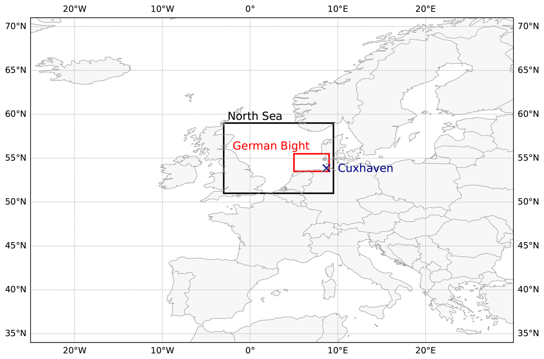
Figure 1 Map with marked areas of the North Sea (black box) and the German Bight (red box). The blue cross indicates the location of Cuxhaven.

In addition to other factors such as atmospheric sea-level pressure and external surges (Böhme et al., 2023), wind proves to be the primary driver for sea-level variability in the German Bight (Dangendorf et al., 2013) and therefore plays an important role in estimating the height of storm surges. Various studies investigate the meteorological conditions that caused extreme storm surges in the past. While they focus on just a few case studies, they demonstrate the successful applicability of reanalysis data for recreating these events: the storm surge studies include the well known Hamburg storm surge of 1962 (Jochner et al., 2013; Meyer and Gaslikova, 2024), one of the highest storm surges ever measured in 1976 (Meyer and Gaslikova, 2024) and the storm surge caused by storm “Xaver” in 2013 (Dangendorf et al., 2016; Meyer and Gaslikova, 2024). While these and other studies focus on the analysis of individual historical events, Krieger et al. (2020) concentrate on the statistics and long-term evolution of German Bight storm activity. They find that storm activity over the German Bight is characterized by multidecadal variability. This is in line with the results of Dangendorf et al. (2014), who find that storm surges in the North Sea are characterized by interannual to decadal variability associated with large-scale atmospheric circulation patterns.

Nevertheless, in order to estimate the resulting storm surge levels in the German Bight, a translation of wind speed into water level is required. Hydrodynamic models are the most widely used and reliable method for translating atmospheric conditions into storm surge estimates. While they provide detailed simulations of storm surges, they are computationally expensive and require extensive input data, making them less suitable for climate simulations. In such cases, simpler approaches, such as statistical methods, can serve as more practical alternatives to analyze storm surges. In particular, the skew surge – the difference between the observed water level and the expected astronomical high-water level – provides reliable information about storm surges (Williams et al., 2016; Ganske et al., 2018). Here, two approaches are commonly employed to translate atmospheric conditions into water levels: one uses the so-called effective wind as a proxy, while the second approach involves predicting skew surges using a statistical model.

For the former, a variable – the effective wind – consisting of wind speed and direction is used to objectively assess the conditions for a storm surge in the German Bight (Müller-Navarra et al., 2003; Jensen et al., 2006). Cuxhaven (Fig. 1), located in the center of the German Bight coast and with its long-gauge data series, is often used as a proxy for that region. For Cuxhaven, the effective wind is defined as the fraction of the 10 m wind blowing from direction 295°. In an empirical study, this wind direction was determined as the one for which the wind-induced increase in water levels in the German Bight is greatest (Müller-Navarra et al., 2003; Jensen et al., 2006). Averaged over the German Bight, the effective wind is therefore a measure of the contribution of wind to storm surges at the German Bight coastline and can be used as an indicator for the storm surge potential of a weather situation (Jensen et al., 2006). Befort et al. (2015) use the effective wind in combination with a storm tracking algorithm to detect storm surges in the German Bight. Using this method, they show an improvement in the identification of storm surge events compared to the sole use of the effective wind. This agrees with findings of Ganske et al. (2018), who state that high effective wind alone is not necessarily linked to a large storm surge height, but that additional parameters such as the storm track need to be taken into account.

Building upon the second approach, namely the use of a statistical model, Müller-Navarra and Giese (1999) re-examined and revised existing studies and similar methods from the 1960s, setting up a statistical model using multiple linear regression in order to determine storm surge situations in the German Bight, i.e., in Cuxhaven. The authors use, as predictors for computing the skew surge in Cuxhaven, wind speed and direction, air and sea surface temperature, air pressure and its 3-hourly change, the water level in Wick on the Scottish east coast 12 h earlier, and water levels in Cuxhaven during the immediately preceding low and high waters. Müller-Navarra and Giese (1999) find that the consideration of external surge and autocorrelation improve the model performance. The result is an empirical model with 14 basic functions that is able to describe the skew surge height in Cuxhaven (Müller-Navarra and Giese, 1999). Several other studies build on this study and base their models on the mathematical approaches by Müller-Navarra and Giese (1999). Jensen et al. (2013), for example, successfully examine the empirical–statistical relationship between wind, air pressure and the skew surge in Cuxhaven for the period 1918 to 2008. As an approximation for external surges, they use air pressure and wind time series at the northern edge of the North Sea. Dangendorf et al. (2014) extend this analysis by reconstructing storm surges in the German Bight back to 1871, but with higher predictive skill from 1910 onward. However, it is worth noting that their model is only based on atmospheric surface forcing as predictors; external surges are excluded from the model setup (Dangendorf et al., 2014). Niehüser et al. (2018) apply a similar model setup for multiple tide gauge locations along the North Sea coast, focusing on the period from 2000 to 2014. In contrast to using wind and air pressure information of the nearest grid cell for each tide gauge location (Jensen et al., 2013; Dangendorf et al., 2014), Niehüser et al. (2018) implement a step wise regression approach, considering time lags up to 24 h. This allows them to determine the location and time lag of relevant predictors for each site. Their model shows comparable skill measures to the more complex model by Jensen et al. (2013). All mentioned statistical modeling approaches require a large number of input variables for very specific locations or regions. Most of these approaches have been employed solely based on observational data or atmospheric reanalysis (Müller-Navarra and Giese, 1999; Jensen et al., 2013; Dangendorf et al., 2014; Niehüser et al., 2018).

In the context of climate change, the assessment of future storm surge risk is of major importance (IPCC, 2023). In order to incorporate necessary climate projections, a less complex statistical model is needed that is applicable to a multi-model ensemble of climate model simulations with only a limited number of variables available and a comparatively coarse spatial resolution.

To fill this gap, this paper seeks to (i) set up a simple storm surge model for Cuxhaven using a multiple linear regression approach based only on the 10 m wind from the ERA5 reanalysis as predictor variable; (ii) improve prediction accuracy and reduce model complexity by applying regularization methods; and (iii) assess the model's performance by using cross-validation methods and classification evaluation. The reason for the restriction to winds is that most climate model simulations provide corresponding information. Thus, this paper introduces a new method for predicting storm surge heights in the German Bight, which can also be applied using data from climate model projections in future studies.

2 Methods and data

We develop a simple storm surge model for the German Bight, i.e., Cuxhaven, based on a multiple linear regression approach and relying exclusively on the grid-cell-specific 10 m effective wind as the predictor variable. Broadly speaking we follow four steps (Fig. 2): (a) data preprocessing (Sect. 2.1.1 and 2.1.2); (b) the identification of the location and lead time of the predictors across the entire North Sea region (namely certain grid cells of the atmospheric reanalysis used; Sects. 2.2 and 3.1); (c) choosing an appropriate threshold value and regularization method for training the model (Sects. 2.3, 3.2 and 3.3); and (d) training and evaluation of the storm surge model (Sects. 2.3, 3.4 and 3.5).

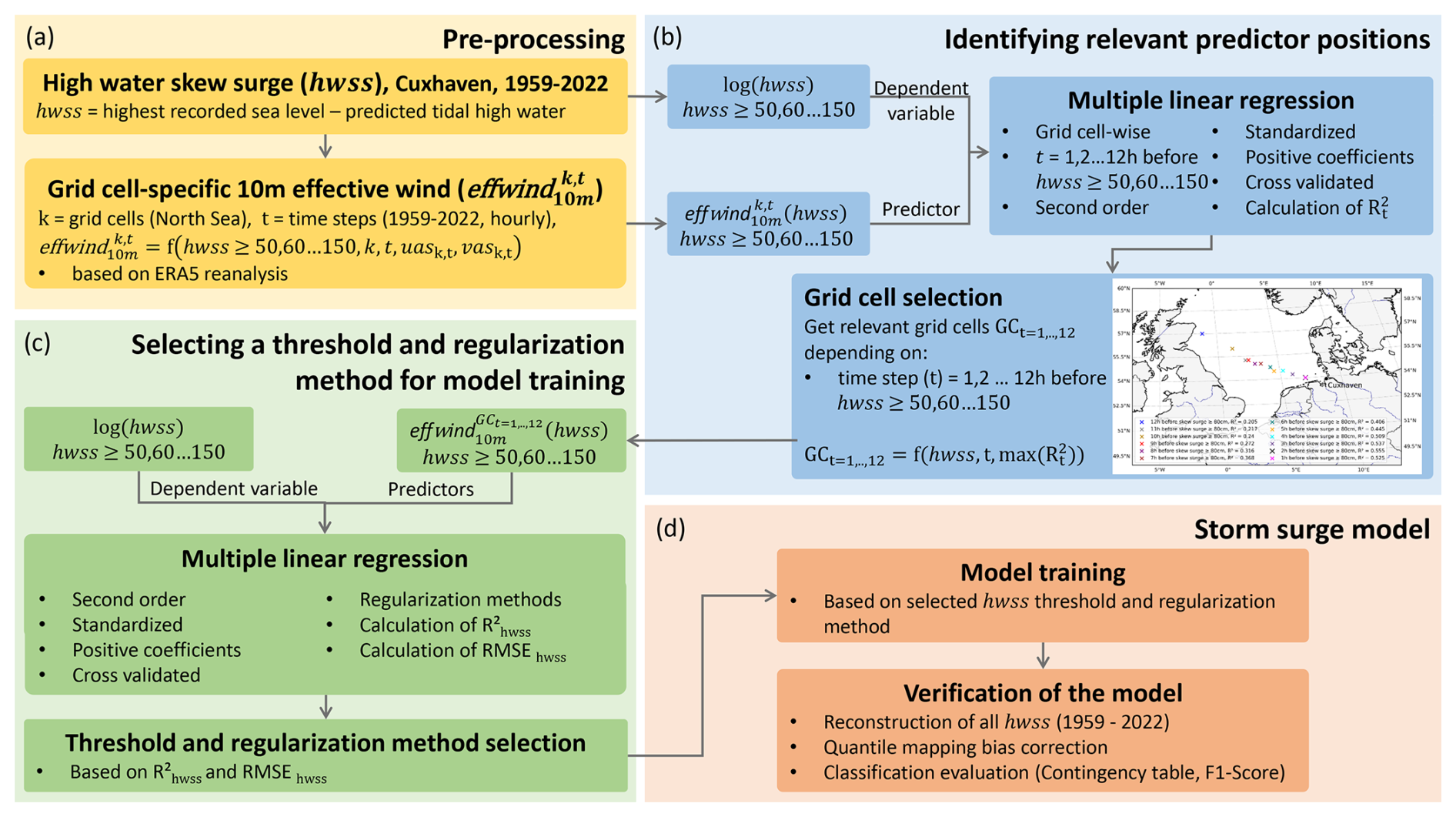
Figure 2 Schematic representation of the process for developing the wind-based storm surge model. Panel (a) shows the data preprocessing steps; panel (b) shows the identification of relevant predictor positions; panel (c) shows the procedure for selecting a threshold and regularization method for model training; panel (d) shows the final model training and evaluation.

2.1 Data

2.1.1 Skew surge data

A valuable metric for storm surge research is the skew surge at high waters (de Vries et al., 1995; Jensen et al., 2013; Williams et al., 2016). It is the height difference between the highest recorded sea level and the predicted tidal high water within a tidal cycle, regardless of the time. We create a time series of high-water skew surge (hwss) at the tide gauge Cuxhaven for the years 1959 to 2022 (Fig. 8). In order to derive hwss, we calculate consistent tidal predictions for these years based on the observed times and water levels of high waters. The observation data are collected and quality checked by the Waterways and Shipping Office Elbe-Nordsee, which operates the Cuxhaven tide gauge. The height reference is tide gauge zero.

We perform tidal analysis and prediction using the method of “harmonic representation of inequalities”. We opt for this method for two reasons: (1) It is a proven operational technique that delivers excellent results under the tidal conditions in the German Bight (Horn, 1960; Boesch and Müller-Navarra, 2019; Boesch and Jandt-Scheelke, 2020), and (2) this technique is applied directly to the heights of the vertices which are needed for this study. For the tidal analysis, we follow the scheme used for the official tide tables: predictions for a given year are based on a tidal analysis of the 19 water-level observation years ending 3 years prior to the prediction year. For example, the prediction for the year 1959 is based on the results of the tidal analysis of the observations from 1938 to 1956. The tidal analysis employs 39 long-period tidal constituents and runs in two iterations, with a three-sigma clipping of outliers before each iteration. We derive the skew surge for 45 162 high waters compared to 45 169 semidiurnal tidal cycles theoretically present in the studied years. It is worth noting that, due to the calculation process, the skew surge data do not take into account sea-level rise.

Table 1 Number of data points for each subsample based on the selected threshold for the period 1959 to 2022.

As this study aims for a storm surge model we only use a subsample of high hwss events for training. As part of this study, we test various thresholds as a lower boundary for defining this subsample, specifically ranging from 50 to 150 cm. We decided on this range as it represents a fair compromise between sample size and the official storm surge definition of greater than or equal to 150 cm above mean high water (Sect. 2.3). In the following we refer to this range as hwss ≥ 50, 60, …, 150 cm. We show the number of available data points for each subsample in Table 1. We describe the choice of the final threshold in Sects. 2.3 and 3.2. As the selected skew surge range is not normally distributed, we apply the natural logarithm to normalize the dataset before using it. Consequently, we train the model based on logarithmic values.

2.1.2 Wind data

ERA5, generated by the European Centre for Medium-Range Weather Forecasts (ECMWF), is the most recent atmospheric reanalysis offering hourly data on various atmospheric, land-surface, and sea-state variables. The data are provided at a horizontal resolution of 31 km and 137 levels in the vertical, covering the period from 1940 onwards (Hersbach et al., 2020).

Based on the 10 m hourly wind components from the ERA5 reanalysis, we use the concept of the effective wind to analyze the wind conditions that contribute to water-level variations in Cuxhaven. The effective wind refers to the combined effect of wind speed and direction. It describes the proportion of the wind projected onto a specific wind direction. Here, the specific wind direction is the one that causes a certain wind-related water level in Cuxhaven. We perform a composite analysis of the zonal (uas) and meridional (vas) components of the 10 m wind, which are associated with hwss ≥ 50, 60, …, 150 cm. For each hour (up to 12 h) prior to the corresponding skew surge event, we use the result of this composite analysis to determine the specific wind direction separately for each hwss training threshold.

As we started our analysis when the backward extension of ERA5 to 1940 was not yet available, we only use the hourly wind components for the period 1959 to 2022. Since our study area is the German Bight, we focus exclusively on the North Sea region, which we define from −5 to 10.5° E in longitude and from 51 to 59° N in latitude. For this region, we count 2079 grid cells. For each of these grid cells (k) and in hourly time steps (t) we calculate the effective wind separately for each hwss training threshold. First, we normalize the mean zonal (${\stackrel{\mathrm{‾}}{\mathrm{uas}}}_k$) and meridional (${\stackrel{\mathrm{‾}}{\mathrm{vas}}}_k$) wind components from the composite analysis by dividing each by the mean wind speed (${\stackrel{\mathrm{‾}}{U}}_k$). We subsequently calculate the effective wind (${\mathrm{effwind}}_{\mathrm{10}\mathrm{m}}^{k,t}\left(\mathrm{hwss}\right)$) by projecting the actual wind components (uas_k,t and vas_k,t) onto the corresponding normalized mean components $\left(\frac{{\stackrel{\mathrm{‾}}{\mathrm{uas}}}_k}{{\stackrel{\mathrm{‾}}{U}}_k}\text{ and }\frac{{\stackrel{\mathrm{‾}}{\mathrm{vas}}}_k}{{\stackrel{\mathrm{‾}}{U}}_k}\right)$:

$$\begin{array}{}\text{(1)}& {\mathrm{effwind}}_{\mathrm{10}\mathrm{m}}^{k,t}\left(\mathrm{hwss}\right)=\left({\displaystyle \frac{{\stackrel{\mathrm{‾}}{\mathrm{uas}}}_k}{{\stackrel{\mathrm{‾}}{U}}_k}}\right)\cdot {\mathrm{uas}}_{k,t}+\left({\displaystyle \frac{{\stackrel{\mathrm{‾}}{\mathrm{vas}}}_k}{{\stackrel{\mathrm{‾}}{U}}_k}}\right)\cdot {\mathrm{vas}}_{k,t}.\end{array}$$

The result is the effective wind for the period 1959 to 2022 in hourly time steps and individually for each grid cell in the North Sea region. The particular feature of ${\mathrm{effwind}}_{\mathrm{10}\mathrm{m}}^{k,t}\left(\mathrm{hwss}\right)$ is the fact that its value can be negative. This is the case as soon as the wind blows from the opposite direction to the specific wind direction.

2.2 Statistical model development

Similar to Niehüser et al. (2018), we apply the approach of non-static predictors, but using a different method. This method only considers predictor locations that are relevant to the observed skew surge variability in Cuxhaven. Thus, instead of just considering the nearest grid cell for the Cuxhaven gauge (Jensen et al., 2013; Dangendorf et al., 2014), we identify grid cells and lead times across the entire North Sea region that are most relevant to the respective subsample (hwss ≥ 50, 60, …, 150 cm). Using the effective wind data up to 12 h before each hwss event, we select the grid cells with the highest relevance at each lead time (further details in Sect. A). This approach enables us to determine the most significant grid cells and lead times for each hwss training threshold (Fig. 2b).

Hereafter, the effective wind in these selected grid cells, along with the corresponding lead times $\left({\mathrm{effwind}}_{\mathrm{10}\mathrm{m}}^{{\mathrm{GC}}_{t=\mathrm{1},\mathrm{\dots },\mathrm{12}}}\left(\mathrm{hwss}\right)\right)$, serve as predictors. We stress that each of the 12 predictor variables represents a specific position and a lead time in the North Sea region. Separately for every subsample (hwss ≥ 50, 60, …, 150 cm), we perform multiple linear regression using each of the three regularization techniques – ridge, lasso and elastic net (further details in Sect. B1). As we count 11 different hwss training thresholds and three regularization methods, we arrive at 33 models. In the following, we refer to these models as skew surge models. We use the standardized ${\mathrm{effwind}}_{\mathrm{10}\mathrm{m}}^{{\mathrm{GC}}_{t=\mathrm{1},\mathrm{\dots },\mathrm{12}}}\left(\mathrm{hwss}\right)$ and set up the skew surge models in quadratic order and with forced positive coefficients (Sect. 2.3). In addition, we determine the respective regularization parameter λ for ridge, lasso and elastic net regression for each skew surge model using cross-validation. Subsequently, we perform a leave-one-out-cross-validation for each skew surge model and regularization technique (Fig. 2c).

2.3 Evaluation and setup of the storm surge model

In order to evaluate the skew surge models (Sect. 2.2), we calculate R² and the root-mean-square error (RMSE) (further details in Sect. B3). Based on these performance metrics, data availability and the ability of the individual skew surge models to capture even very severe storm surges, we decide on one final hwss threshold for model training (Sect. 3.2) and one regularization method (Sect. 3.3). The model trained on the selected hwss subsample using the chosen regularization method is hereafter referred to as the storm surge model.

We evaluate the storm surge model by predicting all hwss, every 12 h, for the years from 1959 to 2022. In doing so, we exclude the year to be predicted from the training. As before, we train the storm surge model based on the subsample corresponding to the previously selected hwss event threshold. Here, the predictors, namely ${\mathrm{effwind}}_{\mathrm{10}\mathrm{m}}^{{\mathrm{GC}}_{t=\mathrm{1},\mathrm{\dots },\mathrm{12}}}\left(\mathrm{hwss}\right)$, are mostly positive, as they correspond to the wind direction relevant to the hwss subsample. For the year that the model is supposed to predict, we have to take all high tides into account. In doing so, we come across skew surge heights that are smaller than the skew surge height with which the model was trained – some even negative. Smaller or sometimes negative hwss indicate a minor water movement or even a water movement away from the coast of Cuxhaven. Here, ${\mathrm{effwind}}_{\mathrm{10}\mathrm{m}}^{{\mathrm{GC}}_{t=\mathrm{1},\mathrm{\dots },\mathrm{12}}}\left(\mathrm{hwss}\right)$, which is mainly responsible for this water movement, tends to take on negative values. Since the storm surge model consists of interaction terms and squared terms, negative ${\mathrm{effwind}}_{\mathrm{10}\mathrm{m}}^{{\mathrm{GC}}_{t=\mathrm{1},\mathrm{\dots },\mathrm{12}}}\left(\mathrm{hwss}\right)$ as predictors would still lead to positive values. This means that despite negative ${\mathrm{effwind}}_{\mathrm{10}\mathrm{m}}^{{\mathrm{GC}}_{t=\mathrm{1},\mathrm{\dots },\mathrm{12}}}\left(\mathrm{hwss}\right)$, the model would predict positive hwss, which is contrary to the physical consequence of negative ${\mathrm{effwind}}_{\mathrm{10}\mathrm{m}}^{{\mathrm{GC}}_{t=\mathrm{1},\mathrm{\dots },\mathrm{12}}}\left(\mathrm{hwss}\right)$. To overcome this problem, we create a mathematical condition that we apply solely to the dataset of the year to be predicted. This mathematical condition specifies that whenever a predictor is negative, the coefficient associated with its squared term becomes negative. Furthermore, if both predictors in an interaction term are negative, the coefficient before the term also becomes negative. This mathematical condition, combined with the forced positive coefficients in the training, allows the model to reproduce the physical consequence of negative ${\mathrm{effwind}}_{\mathrm{10}\mathrm{m}}^{{\mathrm{GC}}_{t=\mathrm{1},\mathrm{\dots },\mathrm{12}}}\left(\mathrm{hwss}\right)$.

However, since we train the model on logarithmic hwss, the model will always predict hwss greater than zero. In order to address this issue, we apply the quantile mapping bias correction technique based on the equations of Cannon et al. (2015). With this method we aim to minimize distributional biases between predicted and observed hwss time series. Its interval-independent approach considers the entire time series, redistributing predicted values based on the distributions of the observed hwss (Fig. 2d).

Moreover, we perform a classification evaluation to investigate whether the model correctly classifies the predicted storm surges according to the storm surge definition for the German North Sea coast. The latter is defined by the height of the water level above mean high water (MHW). According to the definition of the Federal Maritime and Hydrographic Agency (BSH), a storm surge event along the German North Sea coast is classified as follows: an increase in water level of 150 to 250 cm above MHW is referred to as a “storm surge”; if the water level reaches between 250 to 350 cm above MHW, it is classified as a “severe storm surge”; and any event exceeding 350 cm above MHW is referred to as a “very severe storm surge” (Müller-Navarra et al., 2012). To assess the extent to which the storm surge model assigns the predicted hwss to the correct classes, we calculate the F1 score (van Rijsbergen, 1979) (further details in Sect. B2). Specifically, we calculate the F1 score for the classes starting from a storm surge (≥ 150 cm) and from a severe storm surge (≥ 250 cm) for the predicted and bias-corrected high-water skew surges in the years 1959 to 2022.

3 Results

3.1 Identifying relevant predictor positions

In the first step for the development of a storm surge model, we determine the location and lead time of the predictors (${\mathrm{effwind}}_{\mathrm{10}\mathrm{m}}^{k,t}\left(\mathrm{hwss}\right)$) in the North Sea region, individually for each hwss training threshold (hwss ≥ 50, 60, …, 150 cm). Figure 3 shows the location and lead time of the predictors for the training threshold of hwss ≥ 80 cm. 12 h before skew surge events in Cuxhaven, the effective wind in the northwestern section of the North Sea, near Scotland, shows the highest explained variance (R² = 0.205) (blue cross in Fig. 3). With increasing temporal proximity to the skew surge events, the relevance shifts toward the southeastern part of the North Sea. Here, the effective wind in the most southeasterly grid cell, approximately 2 h (R² = 0.555) and 1 h (R² = 0.525) before the skew surge events, provides the best description of the resulting water level in Cuxhaven (black and pink cross in Fig. 3).

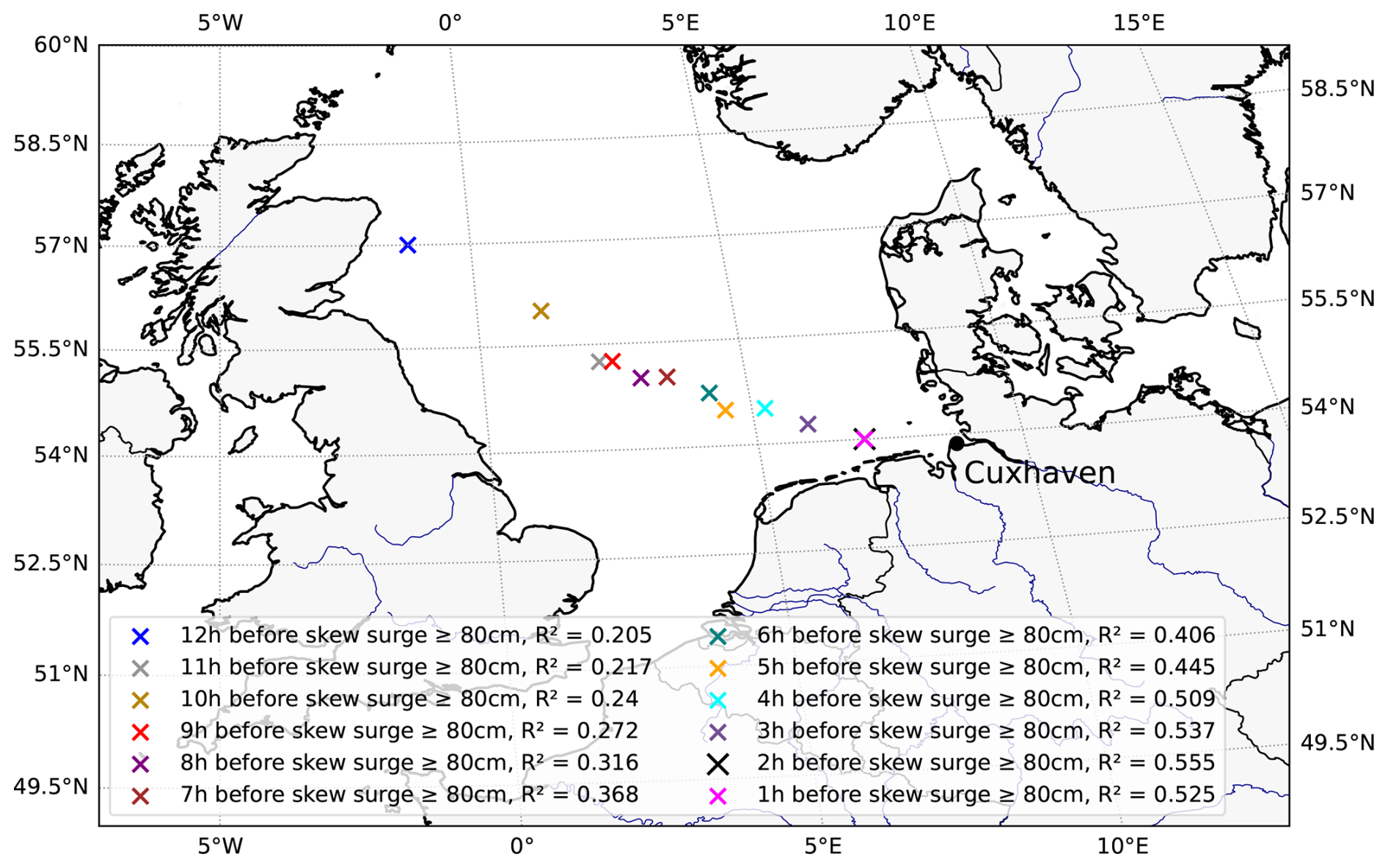
Figure 3 Map of the North Sea region showing the 12 relevant grid cells highlighted with crosses. Each cross represents a specific grid cell, with the color variations indicating the different time intervals before the skew surge event and the corresponding R² value (based on a leave-one-out-cross-validation). The threshold for training is hwss ≥ 80 cm.

Even though the positions in the North Sea region, i.e., the individual grid cells, vary when applying the different hwss subsamples (not shown), the temporal evolution of grid points with maximum R² consistently follows a northwest to southeast progression. This result is in line with findings of Meyer and Gaslikova (2024) and Gerber et al. (2016), who investigate several storm surges and conclude that the northern storm tracks induce high surges across the southern area of the North Sea.

3.2 Selecting a threshold for model training

Once we have determined the location and lead time of the predictors (Sect. 3.1), we create skew surge models by applying the three regularization methods (further details in Sect. B1). We perform a leave-one-out-cross-validation for the models based on ridge, lasso and elastic net regression separately for the training thresholds hwss ≥ 50, 60, …, 150 cm, resulting in three models per hwss training threshold. We assess the performance of these skew surge models by computing R² and RMSE (Fig. 4). We find a general trend of decreasing R² values across all three models as the training threshold increases, with the highest R² value of 0.646 (hwss ≥ 50 cm) and the lowest being 0.569 (hwss ≥ 150 cm) (Fig. 4a). Furthermore, skew surge models using ridge regression have a slightly lower R² value in most cases compared to models using lasso and elastic net regression. Skew surge models based on lasso and elastic net regression show almost equal R² values across all hwss training thresholds (Fig. 4a). This trend is also reflected in the RMSE. When trained with lower hwss thresholds, the RMSE is low and the confidence interval is narrow. Conversely, training with higher hwss thresholds results in higher RMSE values and wider confidence intervals.

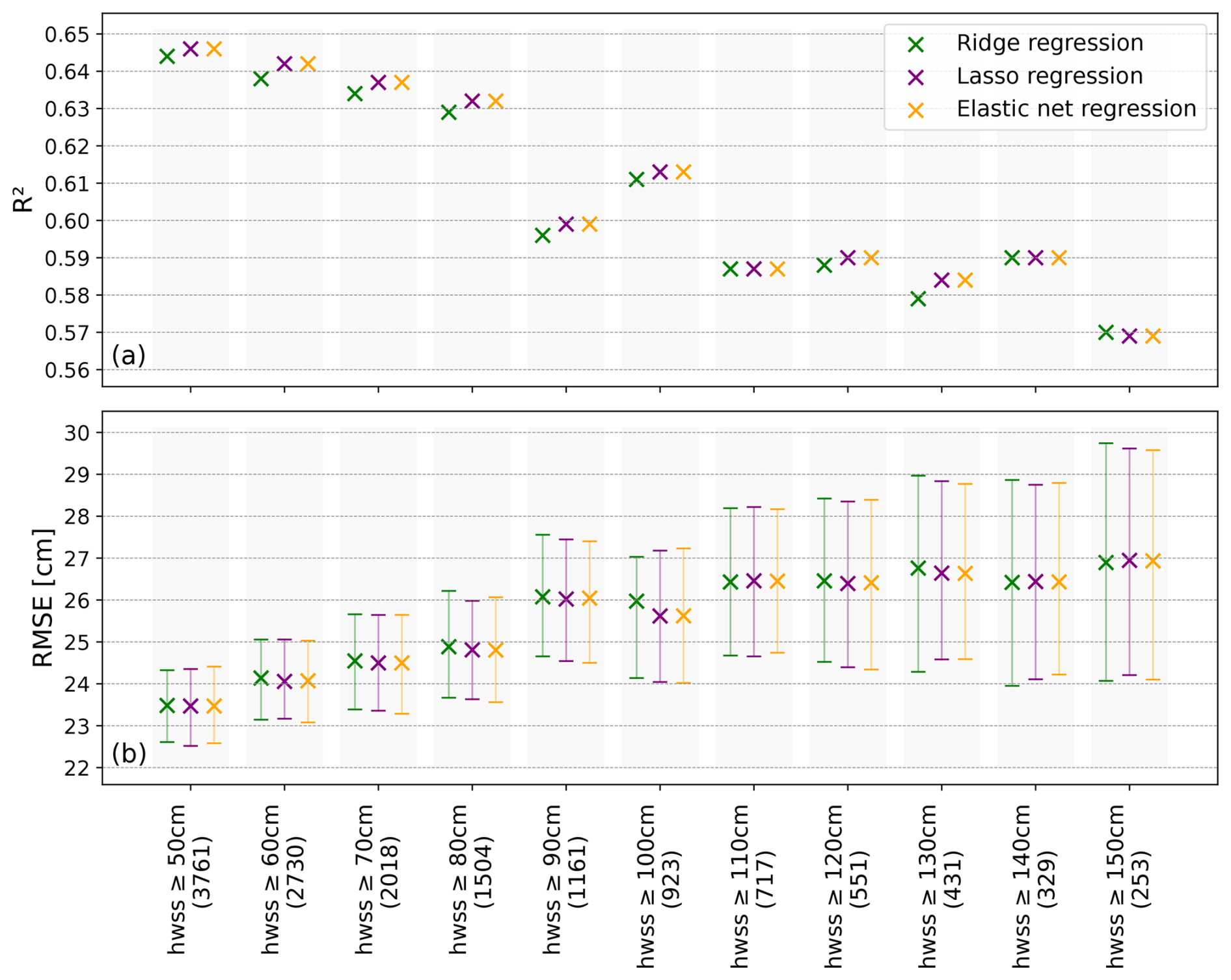
Figure 4 R² (a) and RMSE (b) with the corresponding 95 % confidence intervals of the skew surge models including the different regularization methods across different hwss thresholds for training. The training thresholds are shown on the x axis with the number of available data points in brackets. Each cross represents a specific regularization method (green: ridge regression, purple: lasso regression, orange: elastic net regression). The results are based on a leave-one-out-cross-validation.

Despite lower R² values for models with ridge regression, we find no significant differences in performance compared to the other regularization methods trained on the same threshold. We see this in the fact that the confidence intervals of the models trained with the same hwss threshold value overlap regardless of the regularization method. The similarity in performance of the three models, each with a different regularization method, is the result of forcing the positive coefficients. By forcing positive coefficients, ridge regression reduces certain coefficients to zero if their impact on the accuracy of the prediction is small. This process is similar to predictor selection and results in model behavior similar to lasso and elastic net regression. Consequently, in our case, the performance of ridge regression is closely related to lasso and elastic net regression.

However, when comparing skew surge models across training thresholds, we find that some models trained with higher thresholds (e.g., hwss ≥ 110 cm) perform significantly worse compared to those trained with lower thresholds (e.g., hwss ≥ 50 cm) (Fig. 4b). Additionally, we observe strong fluctuations in the decrease in R² values and the increase in RMSE values, which become visible from a hwss training threshold of hwss ≥ 90 cm (Fig. 4). One explanation for this phenomenon and the partly resulting significant differences in model performance might be the sample size. As the training threshold increases, the number of events decreases. Having sufficient data is essential for the model to learn patterns accurately and ensure better performance on unseen data.

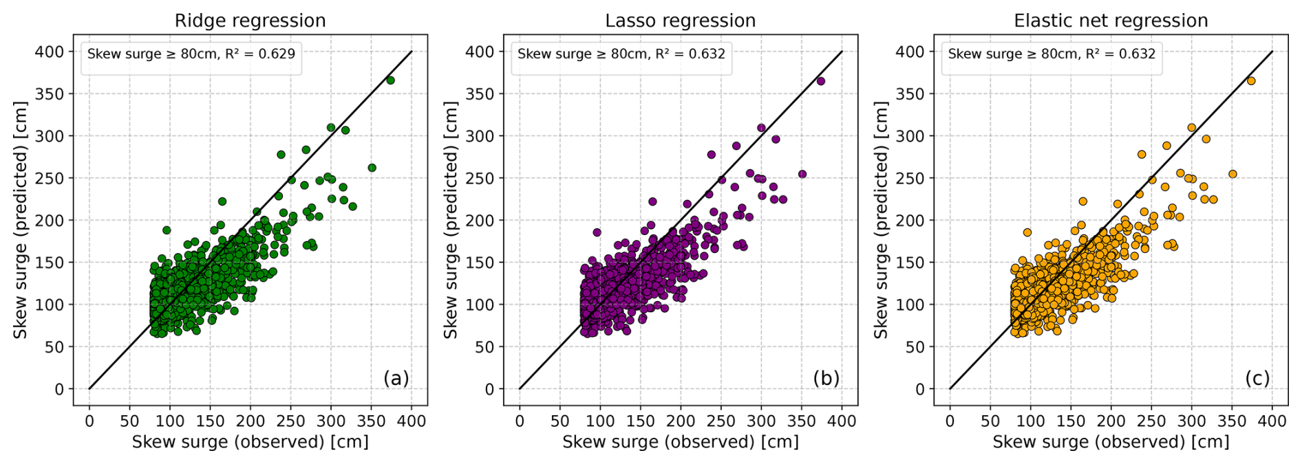
Figure 5 Comparison between observed skew surge heights and predicted skew surge heights resulting from a leave-one-out-cross-validation using ridge (a), lasso (b) and elastic net (c)regression.The black line represents the diagonal, indicating perfect agreement between observed and predicted skew surges. The threshold for training is hwss ≥ 80 cm.

In our pursuit of developing a storm surge model capable of simulating extreme events, we aim to train it using the highest possible hwss threshold. However, when selecting from the number of possible training thresholds, we face the challenge of striking a balance between sample size, high threshold and model performance. We decide to use a hwss training threshold of greater than or equal to 80 cm. We base our decision on the following reasons: (1) this training threshold does not lead to a significant difference in model performance compared to other thresholds (Fig. 4b), (2) we have sufficient data to effectively train the model with this threshold, and (3) we find a satisfactory level of accuracy in simulating extreme events (Fig. 5).

3.3 Selecting a regularization method

Following the selection of a hwss training threshold, the next step is to choose a suitable regularization method. Figure 5 compares the observed and predicted skew surge heights resulting from a leave-one-out-cross-validation using ridge, lasso and elastic net regression, all related to a training threshold of greater than or equal to 80 cm. As mentioned earlier (Sect. 3.2), we observe a similarity in model performance. This is also evident when predicting extremes, with most of the extreme values being underestimated. This could be attributed to the limited data on extreme skew surge events. Moreover, the coarse resolution of the atmospheric forcing (ERA5) may contribute to the underestimation of the most extreme events (Dangendorf et al., 2014; Harter et al., 2024). However, even with a relatively low training threshold (hwss ≥ 80 cm), we still get an appropriate representation of the most extreme events (Fig. 5). The problem of underestimating extreme events is not unique to this study. Several other studies attempting to reconstruct extreme storm surges using statistical models also encounter similar issues (Dangendorf et al., 2014; Niehüser et al., 2018; Harter et al., 2024).

Furthermore, with regard to the performance of the skew surge models, it is important to evaluate the influence of the predictors. As mentioned above (Sect. 3.2), due to forced positive coefficients, ridge regression performs a lasso-like predictor selection, resulting in a sparse model with only seven terms including the intercept. However, lasso and elastic net regression models consist of just five terms in total, including the intercept. Both models show similar performance with identical selected predictors but slightly different coefficients.

In summary, in our case, we observe an overall high level of predictive performance with sparse models. Considering the three potential regression methods, we opt for the elastic net regression model (training threshold hwss ≥ 80 cm) as our final storm surge model (Fig. 5c):

$$\begin{array}{}\text{(2)}& \begin{array}{rl}& {\mathrm{hwss}}_{\mathrm{Storm}\mathrm{Surge}\mathrm{Model}}=\\ & f\left({\mathrm{effwind}}_{\mathrm{10}\mathrm{m}}^{{\mathrm{GC}}_{t=-\mathrm{12}}},{\mathrm{effwind}}_{\mathrm{10}\mathrm{m}}^{{\mathrm{GC}}_{t=-\mathrm{6}}},{\mathrm{effwind}}_{\mathrm{10}\mathrm{m}}^{{\mathrm{GC}}_{t=-\mathrm{2}}},\right.\\ & \left.{\mathrm{effwind}}_{\mathrm{10}\mathrm{m}}^{{\mathrm{GC}}_{t=-\mathrm{1}}}\right)+\mathrm{intercept}.\end{array}\end{array}$$

According to the elastic net regularization, the hwss predicted by the storm surge model is based on the following predictors:

• ${\mathrm{effwind}}_{\mathrm{10}\mathrm{m}}^{{\mathrm{GC}}_{t=-\mathrm{12}}}$: effective wind in the respective grid cell 12 h prior the skew surge event (squared),

• ${\mathrm{effwind}}_{\mathrm{10}\mathrm{m}}^{{\mathrm{GC}}_{t=-\mathrm{6}}}$: effective wind in the respective grid cell 6 h prior the skew surge event (squared),

• ${\mathrm{effwind}}_{\mathrm{10}\mathrm{m}}^{{\mathrm{GC}}_{t=-\mathrm{2}}}$: effective wind in the respective grid cell 2 h prior the skew surge event (squared),

• ${\mathrm{effwind}}_{\mathrm{10}\mathrm{m}}^{{\mathrm{GC}}_{t=-\mathrm{1}}}$: effective wind in the respective grid cell 1 h prior the skew surge event (squared).

This choice is primarily motivated by its simplicity, as it has even fewer terms compared to the ridge regression model and, unlike the lasso regression model, also includes coefficient shrinkage.

3.4 Verification of the storm surge model and quantile mapping bias correction

We eventually verify the storm surge model by using it to predict all high-water skew surge events from 1959 to 2022. By including this broader range of events, we ensure that the model is capable of predicting skew surges on which it was not trained, namely those below 80 cm. In doing so, we train the model based on (hwss ≥ 80 cm) events of all years except the year we want to predict.

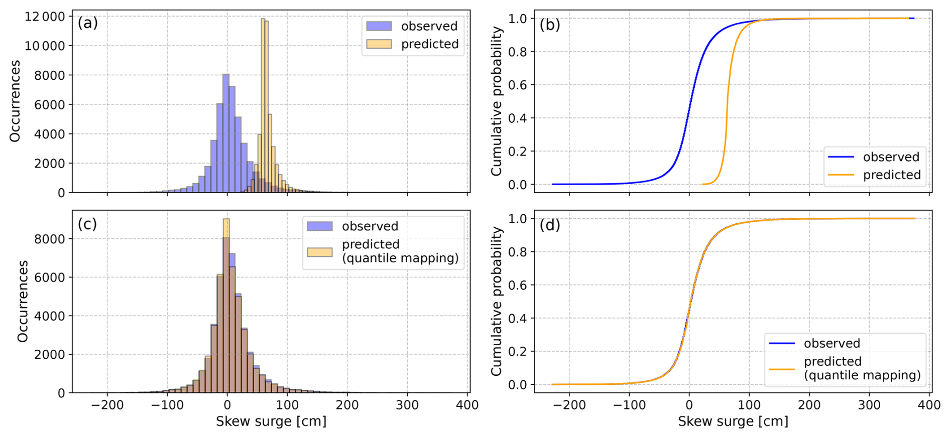
Figure 6 Comparison of all observed (blue) and predicted (orange) PDFs and CDFs of skew surge events from 1959 to 2022, before (a, b) and after (c, d) bias correction. The threshold for training is hwss ≥ 80 cm and the regularization method is elastic net, with the year to be predicted being excluded from the training.

Figure 6a and b show the probability density function (PDF) and cumulative distribution function (CDF) of the observed and predicted skew surge events from 1959 to 2022. The PDF (Fig. 6a) reveals that the observed skew surge data have a broader distribution centered around lower skew surge heights, whereas the predicted skew surge data are more concentrated and centered around greater skew surge heights, never falling below zero. We also see the same pattern in the CDF (Fig. 6b), with the predicted CDF indicating higher skew surges at a given cumulative probability compared to the observed CDF.

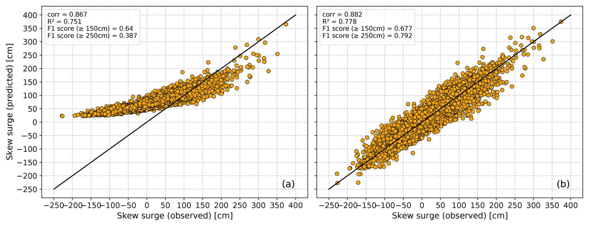
Figure 7 Scatter plots comparing all observed and predicted skew surge heights from 1959 to 2022 – before (a) and after (b) quantile mapping bias correction. The black line represents the diagonal, indicating perfect agreement between observed and predicted skew surges. The threshold for training is hwss ≥ 80 cm and the regularization method is elastic net, with the year to be predicted being excluded from the training.

Additionally, we plot observed against predicted skew surge heights (Fig. 7a) and find a strong correlation coefficient of 0.867 and an R² value of 0.751. However, in the lower range of skew surges (observed values below 80 cm), the model tends to overestimate the values, while in the upper range (observed values above 150 cm), it tends to underestimate the skew surge heights. While the underestimation of extreme skew surges may be due to a lack of data (Sect. 3.2), the overestimation of low or negative skew surges is a consequence of training on logarithmic values. The reason for this lies in the nature of logarithmic functions which is defined only for positive real numbers.

In order to adjust the model output, we apply bias correction using the quantile mapping method of Cannon et al. (2015). We calculate the transfer function using the observed and reconstructed skew surges, but without performing cross-validation. Figure 6c and d show the PDF and CDF of the observed and bias-corrected predicted skew surge events. After applying the quantile mapping bias correction, the predicted distribution aligns much more closely with the observed distribution, both in terms of central tendency and spread. Also, the almost overlapping CDFs (Fig. 6d) and the tighter clustering of points along the diagonal in Fig. 7b indicate that the quantile mapping method successfully corrects the bias in the model's prediction. Moreover, it effectively reduces both the overestimation of lower skew surges and the underestimation of higher skew surges, resulting in better alignment with the observed values. The corrected prediction exhibit a higher correlation with the observed values (corr = 0.882) and an increase in the R² value (R² = 0.778) (Fig. 7b). Compared to the more complex models developed by Jensen et al. (2013), Dangendorf et al. (2014) and Niehüser et al. (2018), our storm surge model demonstrates equally high skill measures despite its extreme simplicity.

3.5 Classification evaluation

To assess the ability of the storm surge model to discriminate extreme storm surge events, we conduct a classification evaluation and calculate the F1 score for two categories: (1) predicting a skew surge of greater than or equal to 150 cm, and (2) predicting a skew surge of greater than or equal to 250 cm. These threshold values are officially used by BSH to define a storm surge and a severe storm surge (Sect. 2.3). To perform the classification evaluation, we use values from the contingency table based on the model's prediction (Table 2). The contingency table consists of four values: true negatives, true positives, false negatives and false positives. We use the last three values to calculate precision, recall and ultimately the F1 score (see Sect. B2 for details), as shown in Fig. 7.

Table 2 Contingency table summarizing model predictions for two categories: skew surge ≥ 150 cm and skew surge ≥ 250 cm. Values in bold black represent bias-corrected predictions, while regular black text indicates predictions without bias correction.

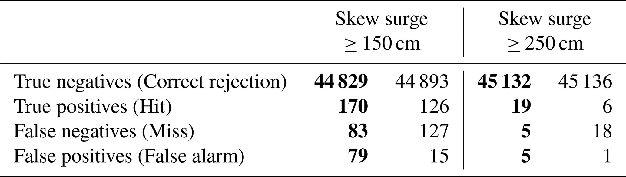
In our analysis, the F1 scores for predicting skew surges greater than or equal to 150 and 250 cm demonstrate a clear improvement after applying bias correction. After bias correction, the F1 scores are 0.677 and 0.792, respectively. In contrast, before bias correction, the F1 scores are 0.64 at the 150 cm threshold and 0.387 at the 250 cm threshold. This indicates good model performance at the 150 cm threshold, showing a reasonable balance between precision and recall. For the higher threshold of 250 cm, the model demonstrates even better performance. This improvement suggests that the model is more accurate and reliable in predicting larger skew surges. However, the very small sample size of just 24 events with a skew surge of more than 250 cm (19 hits and 5 misses) plus five false alarms is associated with much higher uncertainty for the respective F1 score. These results underscore the importance of bias correction, as it significantly enhances the model's ability to predict higher skew surge values, improving both precision and recall for extreme events.

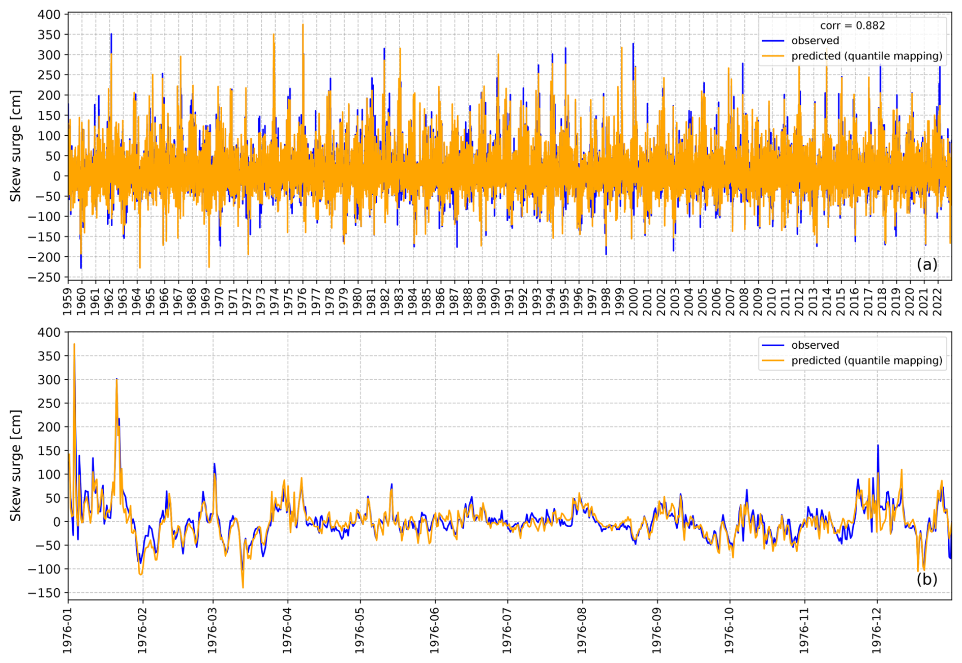
Figure 8 Time series of all observed and predicted (quantile mapping) skew surges from 1959 to 2022 for the entire period (a) and a zoom into the year 1976 for better visibility of particular events in an example year, containing the highest-ever recorded storm surge at Cuxhaven (b). The threshold for training is hwss ≥ 80 cm and the regularization method is elastic net, with the year to be predicted being excluded from the training.

4 Discussion

The presented storm surge model, after bias correction, demonstrates a strong correlation between observed and predicted skew surges (Figs. 7b and 8). The classification evaluation indicates that the model might be even more accurate in predicting higher skew surges (≥ 250 cm) compared to those above 150 cm. Other studies, such as those by Müller-Navarra and Giese (1999), Niehüser et al. (2018) and Dangendorf et al. (2014) often underestimate these higher skew surges. As previously mentioned, the sample size for calculating the F1 score at the 250 cm threshold is very small, so the F1 score is associated with a much greater uncertainty. Nevertheless, the F1 score underlines that the model is effective in predicting extreme events. It is reasonable to assume that especially severe storm surges are predominantly caused by northwesterly winds, as this pattern aligns with the predictor regions (Sect. 3.3; Fig. 3: 12, 6, 2 and 1 h before the storm surge). This assumption is supported by Gerber et al. (2016), who identified, analyzed, and categorized storm surges based on atmospheric conditions. They find that severe storm surges in the German Bight occur more frequently during the northwest type (NWT), characterized by a northwesterly flow from the northern section of the North Sea to the German Bight. Examples of storm surges resulting from an NWT weather situation include the very severe storm surge in February 1962 and the one at the end of January 1976 (Jochner et al., 2013; Gerber et al., 2016; Meyer and Gaslikova, 2024). In these instances, high effective winds (17 to 21 m s⁻¹) are recorded at all predictor locations and our storm surge model successfully predicts these storm surges (Fig. 8). Another weather situation relevant to storm surges in the German Bight is the west and southwest type (W + SWT), characterized by westerly or southwesterly winds (Gerber et al., 2016). Notable examples of storm surges resulting from W + SWT weather situations include the highest storm surges ever recorded at the beginning of January 1976 (Gerber et al., 2016; Meyer and Gaslikova, 2024) and the storm surge in February 2022 (Mühr et al., 2022). Here, our model shows varying performance. On the one hand, with high effective wind speeds (18 to 23 m s⁻¹) at all predictor locations, the storm surge model successfully predicts the storm surge on 3 January 1976 (Fig. 8b). On the other hand, the model underestimates the storm surge in February 2022 (Fig. 8a). In this case, effective wind speeds ranged from 15 to 18 m s⁻¹ in the central (Fig. 3: 6 h before the storm surge) to southeastern sections of the North Sea (Fig. 3: 2 and 1 h before the storm surge), but negative effective winds of −7 m s⁻¹ at the predictor location in the very northwestern section of the North Sea (Fig. 3: 12 h before the storm surge). The influence of the negative effective wind in the northwestern predictor location results in a lower predicted skew surge. However, other external factors may also influence the performance of the model. The storm surge in February 2022 was not only the result of predominantly southwesterly winds but also a part of a series of storms (Mühr et al., 2022). This led to a pre-filling of the North Sea (Mühr et al., 2022), causing weaker effective winds to induce a higher skew surge. This pre-filling effect additionally explains why the model underestimates the February 2022 storm surge. Nevertheless, the resulting skew surge prediction still exceeds 150 cm, which means it is still able to identify an event exceeding this critical threshold operationally used for issuing warnings.

When considering the categories for storm-surge-inducing weather situations, the tracks of the NWT and W + SWT categories overlap in certain areas (Gerber et al., 2016). Thus, we cannot conclusively state that our model is better at predicting storm surges from one category over the other. Nevertheless, as long as the triggering weather situation leads to westerly to northwesterly winds, which is mostly the case, the storm surge model is able to predict the resulting storm surge very well.

Another factor contributing to extreme water levels in the North Sea is external surges. These surges are caused by low-pressure systems over the North Atlantic and are amplified at the continental shelf (Böhme et al., 2023). External surges can cause water-level changes exceeding 1 m along the along the British, Dutch, and German coasts (Böhme et al., 2023). When external surges coincide with storm surges, they have the potential to create extreme water levels. Of the 126 external surges recorded between 1971 and 2020, 21 % occurred during or close to a storm surge event in the German Bight (Böhme et al., 2023). Notable examples of such co-occurrences include the storm surge in February 1962 and the one in December 2013 (Böhme et al., 2023). For both events, the storm surge model predicted a skew surge of more than 150 cm in December 2013 and even more than 250 cm in February 1962 (Fig. 8a), leading to storm surge or severe storm surge warnings. However, the actual water levels were underestimated by approximately 50 cm, which roughly corresponds to the average influence of external surges on water levels in Cuxhaven during storm surges (Böhme et al., 2023).

Despite the aforementioned limitations, we find strong model performance in predicting both moderate and extreme storm surges in the German Bight.

5 Summary and conclusions

In this study, we developed a statistical wind-based storm surge model for the German Bight that is able to predict skew surges based solely on the effective wind. Aiming for model simplicity, we identified predictor locations across the entire North Sea, considered numerous training thresholds, and applied three different regularization methods. The resulting storm surge model comprises only five terms: the squared effective wind in certain grid cells at four lead times (12, 6, 2, and 1 h prior to the skew surge event) as robust predictors, along with an intercept.

We validate the model against historical data and find that it achieves high predictive accuracy, rivaling more complex models despite its simplicity. Moreover, our findings underscore the significance of wind as the primary driver of storm surges in the German Bight. The model provides reliable predictions for both moderate and extreme storm surge events, with more accurate predictions for surges preceded by westerly or northwesterly winds. In particular, the good prediction accuracy for storm surges greater than or equal to 250 cm is a unique outcome of this study.

Furthermore, the simplicity of our storm surge model facilitates its application to climate simulations, making it a valuable tool for assessing storm surge risk in the German Bight under changing climate conditions, on top of sea-level rise. Additionally, this approach is not only effective for the German Bight but also adaptable to other coastal regions worldwide.

Appendix A: Identifying relevant predictor positions

To determine the location and lead time of the predictors (${\mathrm{effwind}}_{\mathrm{10}\mathrm{m}}^{k,t}\left(\mathrm{hwss}\right)$) within the North Sea region, we create an individual statistical model for each grid cell in the North Sea region at each time step using quadratic regression. In the following, we refer to these models as grid-cell models. In a first step, we select all time steps of ${\mathrm{effwind}}_{\mathrm{10}\mathrm{m}}^{k,t}\left(\mathrm{hwss}\right)$ 12 h before the respective occurrence of hwss ≥ 50, 60, …, 150 cm in Cuxhaven. Since ${\mathrm{effwind}}_{\mathrm{10}\mathrm{m}}^{k,t}\left(\mathrm{hwss}\right)$ is available in hourly resolution, this corresponds to 12 time steps. We choose 12 h, as this is approximately the time between two high tides. Since we count 2079 grid cells in the North Sea region and consider 12 time steps, we have a total of 24 948 grid-cell models for each of the 11 hwss training thresholds. The dependent variable in each model is the respective logarithmic hwss height, with the standardized ${\mathrm{effwind}}_{\mathrm{10}\mathrm{m}}^{k,t}\left(\mathrm{hwss}\right)$ serving as predictor. As the wind stress depends on the square of the wind speed (Olbers et al., 2012), we create the grid-cell models with quadratic order.

Once we have defined the conditions for the grid-cell models, we perform a leave-one-out-cross-validation and calculate the coefficient of determination (R²) for each grid-cell model. In order to obtain the most relevant grid cells for the respective subsample of events, we select the grid-cell model with the highest R² value from each time step (Fig. A1). As we consider the 12 h before the occurrence of hwss ≥ 50, 60, …, 150 cm, we obtain 12 grid-cell models and thus grid cells (${\mathit{\text{GC}}}_{t=\mathrm{1},\mathrm{\dots },\mathrm{12}}$), each of which contains both the relevant lead time and position in the North Sea region for the respective hwss training threshold in Cuxhaven.

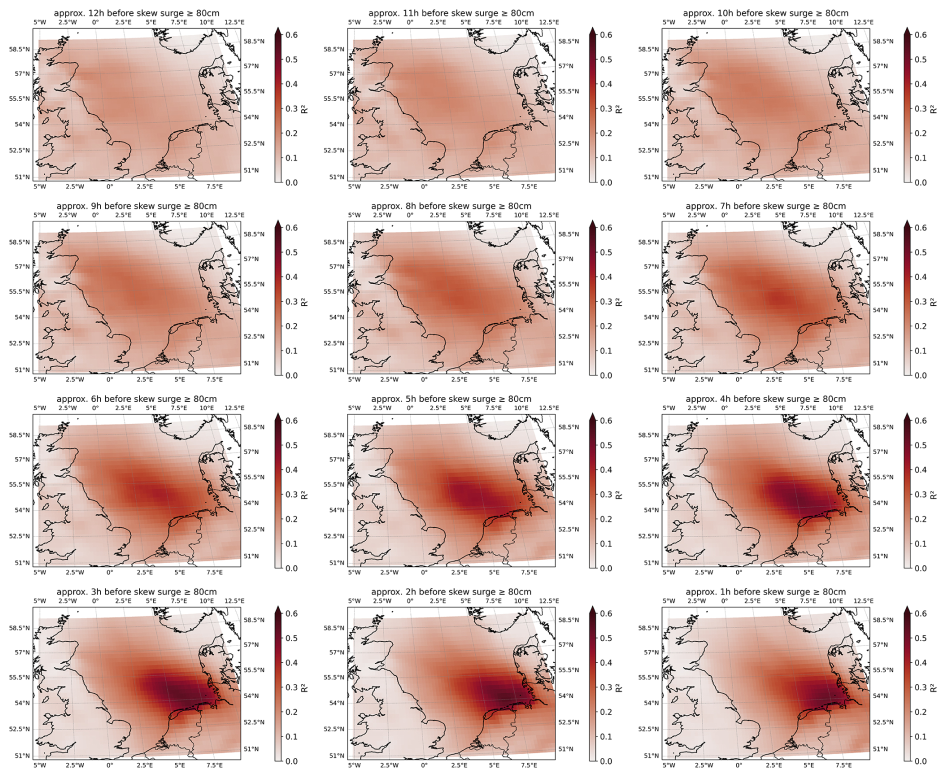
Figure A1 R² value (based on a leave-one-out-cross-validation) of each grid-cell model within the North Sea region for 12 h before the skew surge event (top left) to 1 h before the skew surge event (bottom right). The darker the color, the greater the R² value. The event threshold for training is hwss ≥ 80 cm.

Appendix B: Performance metrics and model optimization strategies

B1 Regularization methods

The usual regression procedure for determining the unknown coefficients in a multiple linear regression model is based on the ordinary least squares (OLS) method. Its error criterion is the minimization of the sum of the squared errors, where the error is the difference between the actual and the predicted value (Wilks, 2011). However, OLS has some known disadvantages. For example, OLS is highly sensitive to outliers in the data and can be prone to overfitting. In addition, OLS performs poorly when it comes to accuracy in predicting unseen data and in interpreting the model (Zou and Hastie, 2005). For the latter, the simpler the model, the more the relationship between the dependent variable and the predictors is highlighted. The model's simplicity is particularly important when the number of predictors is large.

An effective method for overcoming the difficulties of OLS is regularization. It is a method to avoid overfitting and control the complexity of models by adding a penalty term to the model's target function during training. The aim is to keep the model from fitting too closely to the training data and to encourage simpler models that are better suited to unseen data. Here, we consider three different regularization techniques, namely ridge (Hoerl and Kennard, 1970a, b), lasso (Tibshirani, 1996) and elastic net regression (Zou and Hastie, 2005).

The main idea behind ridge regression (Hoerl and Kennard, 1970a, b) is its ability to strike a balance between bias and variance. This is achieved by including a penalty term proportional to the square of the coefficients in the loss function. This approach leads to the coefficient estimates being smaller while still having non-zero values. The target function to be minimized becomes:

$$\begin{array}{}\text{(B1)}& {\mathrm{Loss}}_{\mathrm{Ridge}}={\mathrm{Loss}}_{\mathrm{OLS}}+\mathit{\lambda }\sum _{j=\mathrm{1}}^n{\mathit{\beta }}_j^{\mathrm{2}},\end{array}$$

where Loss_OLS is the loss function of Ordinary Least Squares, λ is the regularization parameter that defines the regularization strength and ${\sum }_{j=\mathrm{1}}^n{\mathit{\beta }}_j^{\mathrm{2}}$ is the regularization term – the sum of squared coefficients. Since large coefficients may lead to low bias and high variance, they are penalized by adding the regularization term and effectively shrink toward zero. Consequently the model becomes sensitive to fluctuations in the data. However, ridge regression is unable to create a simple model, in the sense of fewer predictors, as it always retains all predictors in the model. This contrasts with the lasso regression (Tibshirani, 1996).

Lasso regression is a method to reduce overfitting and perform predictor selection by setting some coefficient estimates to exactly zero. For this purpose, a regularization term proportional to the absolute value of the coefficients is added to the loss function. The target function to be minimized becomes:

$$\begin{array}{}\text{(B2)}& {\mathrm{Loss}}_{\mathrm{Lasso}}={\mathrm{Loss}}_{\mathrm{OLS}}+\mathit{\lambda }\sum _{j=\mathrm{1}}^n\left|{\mathit{\beta }}_j\right|,\end{array}$$

where Loss_OLS is the OLS loss function, λ is the regularization parameter and ${\sum }_{j=\mathrm{1}}^n\left|{\mathit{\beta }}_j\right|$ is the regularization term – the sum of absolute values of coefficients. Lasso regression simplifies the model by shrinking less important coefficients to zero, effectively eliminating some predictors from the model. This leads to simpler and more interpretable models.

Zou and Hastie (2005) propose a third regularization method whose main principle is to balance ridge and lasso regression by adding both ridge and lasso regularization terms to the loss function. The target function to be minimized becomes:

$$\begin{array}{}\text{(B3)}& {\mathrm{Loss}}_{\mathrm{Elastic}\mathrm{Net}}={\mathrm{Loss}}_{\mathrm{OLS}}+{\mathit{\lambda }}_{\mathrm{1}}\sum _{j=\mathrm{1}}^n\left|{\mathit{\beta }}_j\right|+{\mathit{\lambda }}_{\mathrm{2}}\sum _{j=\mathrm{1}}^n{\mathit{\beta }}_j^{\mathrm{2}},\end{array}$$

where Loss_OLS is the loss function of OLS, λ₁ and λ₂ are the regularization parameters for lasso and ridge penalties, respectively, ${\sum }_{j=\mathrm{1}}^n\left|{\mathit{\beta }}_j\right|$ is the lasso regularization term and ${\sum }_{j=\mathrm{1}}^n{\mathit{\beta }}_j^{\mathrm{2}}$ is the ridge regularization term. Elastic net regression combines the strength of both lasso and ridge regression by balancing the selection of predictors and coefficient shrinkage, resulting in more robust and reliable predictive models.

B2 F1 score

The F1 score combines precision and recall into one metric. Precision measures the accuracy of positive predictions made by the model. It is determined by dividing the number of true positive predictions by the total number of samples predicted as positive, regardless of correct identification:

$$\begin{array}{}\text{(B4)}& \mathrm{Precision}={\displaystyle \frac{\mathrm{TP}}{\mathrm{TP}+\mathrm{FP}}},\end{array}$$

where TP represents true positive predictions and FP indicates false positive predictions.

Recall measures the fraction of actual positives that were correctly identified by the model. It is computed by dividing the number of true positive predictions by the total number of samples that should have been identified as positive:

$$\begin{array}{}\text{(B5)}& \mathrm{Recall}={\displaystyle \frac{\mathrm{TP}}{\mathrm{TP}+\mathrm{FN}}},\end{array}$$

where TP refers to true positive predictions and FN to false negative predictions. The F1 score is defined as the harmonic mean of precision and recall:

$$\begin{array}{}\text{(B6)}& F\mathrm{1}=\mathrm{2}{\displaystyle \frac{PR}{P+R}},\end{array}$$

where P stands for precision and R for recall. The F1 score has its best value at 1 (perfect precision and recall) and its worst at 0.

B3 Root-mean-square error

The root-mean-square error (RMSE) is a measure of how well the model is performing in terms of prediction accuracy, with lower values indicating better performance. It has the same units as the observed values – in this case cm. We also determine the 95 % confidence interval for the RMSE by applying the bootstrap method. This method involves resampling from the original dataset – here 1000 times – with replacements to simulate multiple scenarios.