the Creative Commons Attribution 4.0 License.
the Creative Commons Attribution 4.0 License.
 | 08 Aug 2024
Risk-informed representative earthquake scenarios for Valparaíso and Viña del Mar, Chile
Mauricio Monsalve
Juan Camilo Gómez Zapata
Elisa Ferrario
Alan Poulos
Juan Carlos de la Llera
Daniel Straub
Different risk management activities, such as land-use planning, preparedness, and emergency response, utilize scenarios of earthquake events. A systematic selection of such scenarios should aim at finding those that are representative of a certain severity, which can be measured by consequences to the exposed assets. For this reason, defining a representative scenario as the most likely one leading to a loss with a specific return period, e.g., the 100-year loss, has been proposed.
We adopt this definition and develop enhanced algorithms for determining such scenarios for multiple return periods. With this approach, we identify representative earthquake scenarios for the return periods of 50, 100, 500, and 1000 years in the Chilean communes of Valparaíso and Viña del Mar, based on a synthetic earthquake catalog of 20 000 scenarios on the subduction zone with a magnitude of Mw≥5.0. We separately consider the residential-building stock and the electrical-power network and identify and compare earthquake scenarios that are representative of these systems. Because the representative earthquake scenarios are defined in terms of the annual loss exceedance rates, they vary in function of the exposed system. The identified representative scenarios for the building stock have epicenters located not further than 30 km from the two communes, with magnitudes ranging between 6.0 and 7.0. The epicenter locations of the earthquake scenarios representative of the electrical-power network are more spread out but not further than 100 km away from the two communes, with magnitudes ranging between 7.0 and 9.0. For risk management activities, we recommend considering the identified scenarios together with historical events.
- Article
(7375 KB) - Full-text XML
- BibTeX
- EndNote


Due to the complexity of earthquake events and the response of infrastructure and society to these events, risk managers analyze potential impacts of strong seismic events and test risk management capacities through representative earthquake scenarios (e.g., Salgado-Gálvez et al., 2018; Aguirre et al., 2018). Scenario-based analysis enables the modeling and simulation of the complex processes and interactions during and after earthquake events, with a level of detailing that is not possible through a complete probabilistic hazard and risk analysis. As such, the earthquake scenarios are the starting point for such a more detailed risk assessment and for recommendations for improving risk management (e.g., Chatelain et al., 1995; Feliciano et al., 2023).
Representative scenarios are commonly selected based on expert knowledge (e.g., Aguirre et al., 2018) and past events (e.g., Indirli et al., 2011). Synthetic seismic catalogs have also been used for the selection of representative scenarios (McGuire, 1995; Jayaram and Baker, 2009b; Miller and Baker, 2015). A particular approach for scenario selection is based on hazard disaggregation (Bazzurro and Cornell, 1999), which utilizes the conditional probability of different hazard scenarios given an intensity measure (e.g., peak ground acceleration, PGA) at a specific site of interest either equaling or exceeding a threshold (Fox et al., 2016; Fox, 2023). As its name suggests, classic hazard disaggregation does not explicitly consider the losses of the affected engineering systems, which are often a function of the intensity measures at multiple locations and which are subject to uncertainty.
The above concepts were extended to loss disaggregation to find earthquake scenarios in terms of magnitude and hypocentral distance that exceed a loss threshold for residential-building stocks (Goda and Hong, 2009) or infrastructure (Jayaram and Baker, 2009b). Because the spatially accumulated loss can be defined for any portfolio of buildings and infrastructure, loss disaggregation implicitly considers spatially distributed intensity measures. Rosero-Velásquez and Straub (2022) proposed a definition of a representative hazard scenario associated with a loss of return period t, e.g., the 100-year loss, which in general does not correspond to the magnitude or intensity measure of the same return period. It is defined as the most likely scenario that leads to the loss value (i.e., its occurrence) associated with this return period t. They also presented a numerical procedure for selecting the representative hazard scenario in a continuous space of source parameters with a surrogate model and active learning, thus considering the uncertainty in the conditional losses given a hazard scenario. In the context of seismic risk analysis, earthquake scenarios that are representative of t-year loss can be different for different engineering systems, even if they are located in the same area. The definition of Rosero-Velásquez and Straub (2022) differs from the loss disaggregation presented by Goda and Hong (2009) and Jayaram and Baker (2009b) because the latter define the representative scenario as the most likely one to exceed the t-year loss. In this contribution, we compare the two definitions and argue that a definition in terms of the occurrence of the t-year loss is more appropriate for most applications, in line with the findings of Fox et al. (2016) for hazard disaggregation.
Considerable work has been devoted to the study of the seismic hazard, vulnerability, and risk in the Valparaíso coastal area of Chile due to its high population density and economic importance in combination with strong seismic activity. Recent earthquakes that led to significant damage occurred in 1971 with Mw=7.8, in 1985 with Mw=8.0 (Indirli et al., 2011), and in 2010 with Mw=8.8 (de la Llera et al., 2017). Recent studies on the Valparaíso area deal with seismic characterization (e.g., Carvajal et al., 2017; Candia et al., 2020), source models (e.g., Poulos et al., 2019; Pagani et al., 2021), ground motion models (Montalva et al., 2017), building exposure models (e.g., Yepes-Estrada et al., 2017; Jiménez et al., 2018; Gómez-Zapata et al., 2022b, b), damage analysis on individual buildings (e.g., Indirli et al., 2011; Jünemann et al., 2015), socio-economic impact (Jiménez Martínez et al., 2020), and the seismic risk analysis of the electrical-power network (Ferrario et al., 2022) and road network (Allen et al., 2022). Additionally, Indirli et al. (2011) identified representative earthquake scenarios using historical events and expert knowledge for generating representative ground motion time series but solely from the hazard point of view and disregarding the risk component.
This paper determines representative earthquake scenarios for different return periods for the residential-building stock and the power supply network in the communes of Valparaíso and Viña del Mar. We adapt and extend the methodology described by Rosero-Velásquez and Straub (2022) for identifying scenarios associated with different return periods from a synthetic earthquake catalog. The representative scenario is found directly by solving a stochastic optimization problem, namely the identification of the mode of the conditional distribution of the source parameters given the occurrence (or exceedance) of the t-year loss among the scenarios in the catalog. The stochastic optimization problem is solved with an active-learning strategy, whereby the uncertainty in the objective function is estimated by bootstrapping.
We introduce the definition of a representative earthquake scenario more formally in Sect. 2. Then we present the methodology for computing the scenarios on a seismic catalog in Sect. 3 and illustrate it with idealized examples in Sect. 4. The description of the study area and the utilized hazard and system models are presented in Sect. 5. The results are given in Sect. 6 and discussed in Sect. 7. In the paper, we employ the notation and acronyms summarized in Appendix A.
An earthquake scenario can be described by a vector θ of source parameters, including the magnitude; hypocentral distance; and source longitude, latitude, and depth. In a stochastic model, the scenario is a single realization of a random vector Θ, with joint probability density function (PDF) fΘ(θ). The PDF of Θ is obtained from one or more seismic source models (e.g., Poulos et al., 2019) and is conditioned on the occurrence of a seismic event, whose frequency (occurrence rate) is λH.
An earthquake catalog is a set of n earthquake scenarios of , which are realizations of Θ. The catalog can be a set of synthetic earthquake scenarios, obtained by random sampling from fΘ(θ). Alternatively, the catalog can be obtained from past events (e.g., Poulos et al., 2019).
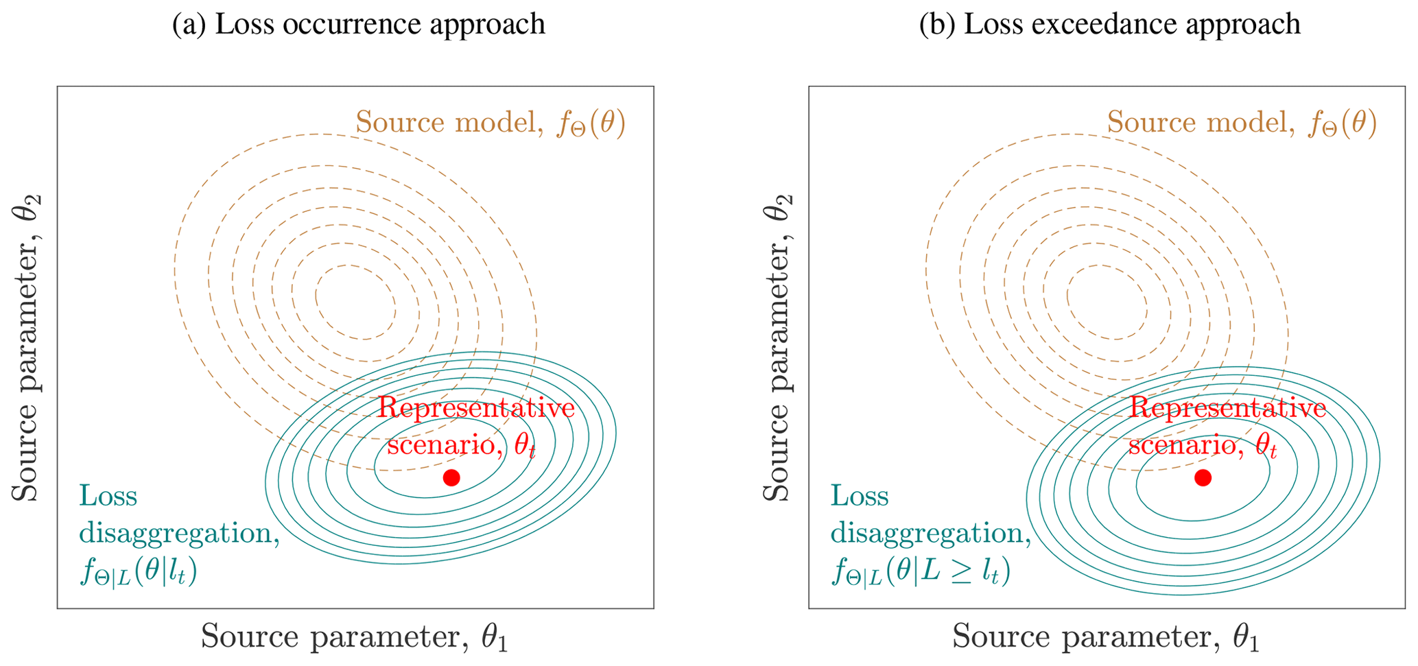
Figure 1Illustration of the representative scenario in the source parameter space, modified after Rosero-Velásquez and Straub (2022), in terms of loss occurrence (a) and in terms of loss exceedance (b).
Synthetic earthquake catalogs have been used in event-based probabilistic seismic hazard analysis (PSHA) and earthquake risk assessment (e.g., Salgado-Gálvez et al., 2018; Ferrario et al., 2022; Allen et al., 2022). The aim of PSHA is to obtain the occurrence rate and distribution of ground motions, taking into account all possible earthquake scenarios (Cornell, 1968; Esteva, 1970), and event-based PSHA utilizes Monte Carlo simulation for sampling earthquake scenarios. Similarly, event-based earthquake risk assessment on spatially distributed systems utilizes synthetic earthquake scenarios for computing the losses, considering the spatial correlation in the ground motion and the vulnerability of the exposed assets (Baker et al., 2021).
For a given earthquake scenario, ground motion models (GMMs) result in spatially distributed intensity measures, e.g., PGA and spectral accelerations, which are input to assess the losses associated with the exposed systems. In the general case, these predictions are stochastic. Thereafter, the model of the engineering system considers the physical and functional vulnerability and results in a loss value L.
Because of the randomness and uncertainty in the earthquake scenario, GMM, vulnerabilities, and exposure, L is a random variable whose cumulative distribution function (CDF) FL(l) can be obtained by performing an event-based earthquake risk assessment for spatially distributed systems with the synthetic earthquake catalog. By combining this CDF with the earthquake occurrence rate λH, one obtains the loss exceedance function λL(l):
Based on the loss exceedance function, the losses lt with a specific return period t can be found as
which is defined only for . The loss lt is also called the t-year loss.
Following Rosero-Velásquez and Straub (2022), the representative earthquake scenario θt, associated with a return period t, is defined as the most likely scenario among those causing the t-year loss lt. In other words, θt is the mode of the conditional PDF of Θ given the loss L=lt, also called the loss disaggregation of Θ given L=lt:
wherein returns the point at which the objective function has a maximum. Equation (3) defines the representative earthquake scenario by conditioning on the occurrence of the loss lt, whereby lt is defined in terms of the exceedance rate. The equation describes the scenario that is most likely to lead to the t-year loss lt.
An alternative definition can be formulated in terms of loss exceedance instead of loss occurrence:
Equation (4) defines the scenario that is most likely to exceed lt. This is the definition corresponding to the classical loss disaggregation (Goda and Hong, 2009; Jayaram and Baker, 2009b). We note that with this definition, in general, the scenario representative of a t-year loss will have a return period higher than t. Hence, we find its interpretation more difficult and prefer the definition in Eq. (3). Nevertheless, we propose algorithms to evaluate the representative scenarios according to the two definitions and compare the resulting scenarios in an illustrative example.
Figure 1 illustrates the conditional distributions fΘ|L(θ|lt) and fΘ|L(θ|L≥lt) for two source parameters , e.g., representing the magnitude Mw and the hypocentral distance R with respect to a location of interest.
By Bayes' rule, Eq. (3) can be expressed in terms of fΘ(θ),
and similarly for the loss exceedance approach,
wherein fL|Θ(l|θ) and FL|Θ(lt|θ) are, respectively, the conditional PDF and CDF, illustrating that the scenario selection criterion balances the probability of the earthquake scenario (quantified by fΘ(θ)) and the probability of the t-year losses occurring (or being exceeded) at that scenario.
To ease the notation in the following section, we let zt(θ) denote the objective function of Eq. (5),
and denote the objective function of Eq. (6),
We consider the case where the randomness of earthquake events is represented through a synthetic earthquake catalog. Specifically, we aim at identifying the earthquake scenarios in the catalog that maximize the objective function in Eqs. (5) and (6) for different return periods t.
The objective functions of Eqs. (5) and (6) consist of the PDF fΘ(θ), which is known from the earthquake source model, and the conditional PDF or CDF of L given Θ evaluated at lt, which can be approximated with conditional samples of losses. To account for the aleatory uncertainty in the modeled ground motions one can draw Monte Carlo samples from the catalog (Silva, 2016) and propagate them to the loss metrics. However, performing this number of loss evaluations for an entire seismic catalog (normally containing dozens of thousands of events) is computationally (too) expensive. As an alternative, one can use Gaussian process models in combination with active learning to handle aleatory uncertainty more efficiently (Tomar and Burton, 2021; Rosero-Velásquez and Straub, 2022). Furthermore, pre-selecting scenarios by the use of extreme value theory and the generalized Pareto distribution (Borzoo et al., 2021) has been proposed.
We propose first performing only one loss evaluation for each scenario in the catalog and using these to approximate the loss exceedance function and lt. The same samples are used for an initial approximation of fL|Θ(lt|θ), the second part of the objective function. This approximation is improved by the use of active learning to identify earthquake scenarios in the catalog for which additional loss evaluations are to be performed.
This methodology is an adaptation of the one proposed in Rosero-Velásquez and Straub (2022).
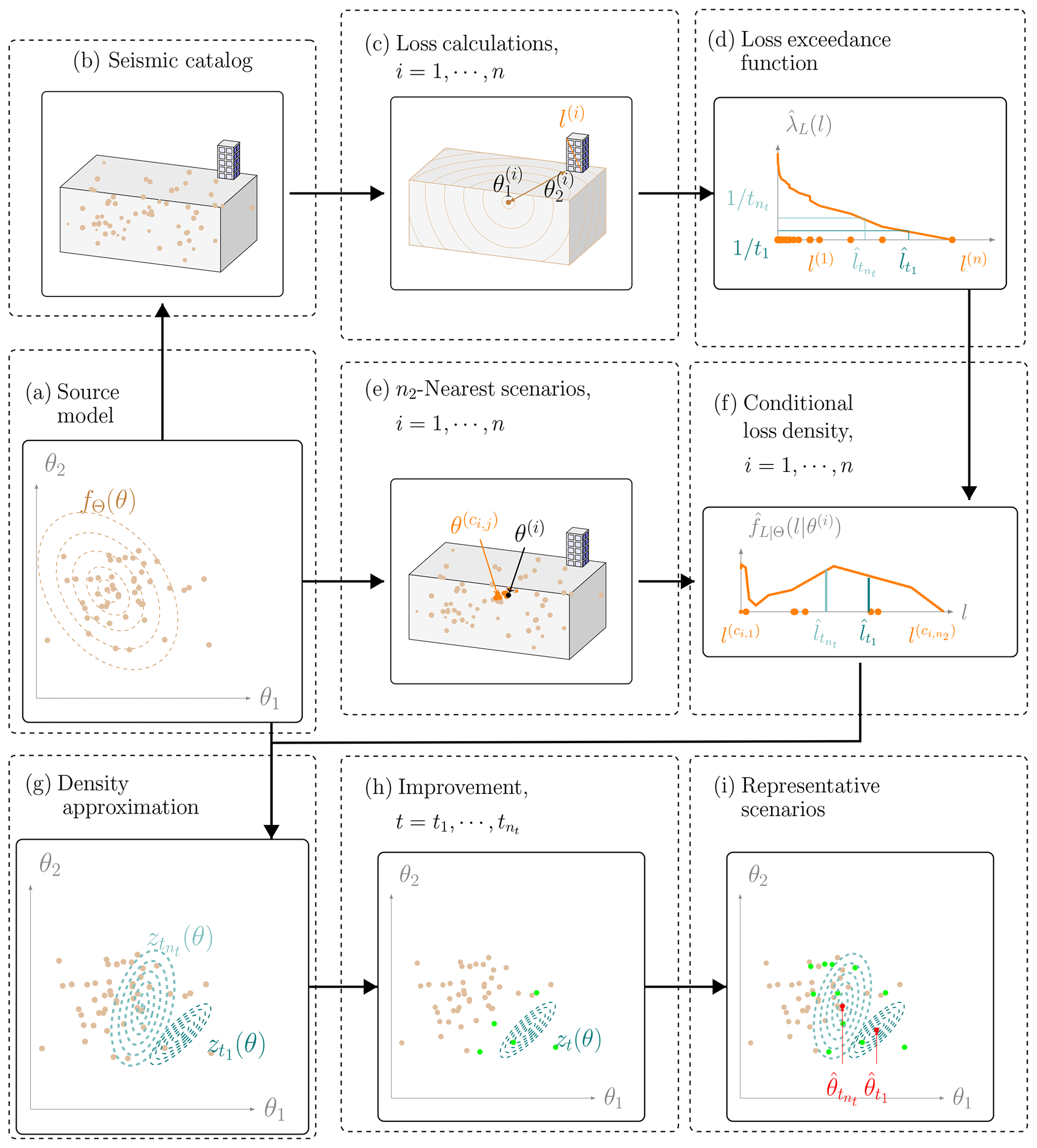
Figure 2General procedure for selecting representative earthquake scenarios with a synthetic earthquake catalog in terms of loss occurrence. Section 3.1 explains panels (e) and (f) in more detail, and Sects. 3.3 and 3.4 explain panel (h). The remaining panels are referred to in Sect. 3. The procedure in terms of loss exceedance only differs in panel (f), and it is explained in Sect. 3.2.
Figure 2 illustrates the main steps of the methodology for selecting representative earthquake scenarios for nt return periods . The earthquake model in this example is a single seismic source within a bounding volume, and the system is a single building.
The starting point is a seismic source model (Fig. 2a), which consists of the occurrence rate λH and the PDF of the source parameters fΘ(θ), together with an associated stochastic seismic catalog (Fig. 2b). The catalog consists of a set of n random and independent earthquake scenarios generated from fΘ(θ), possibly associated with weights with . The generation of such catalogs for the study site is described in Sect. 5.2.
For each scenario, one simulates the ground motion fields in terms of the intensity measure (e.g., the peak ground acceleration, PGA) through the GMM. These intensity measures are the input to assess the performance of the system components by combining them with vulnerability functions. Based on the component performances, the total losses in the system l are evaluated (Fig. 2c). Details on the simulation of the ground motion, the system response, and loss calculation for the study site are given in Sect. 5.
From these samples of the system losses, one obtains an estimate of the loss exceedance curve :
where is the indicator function. In addition, one obtains estimates of the t-year losses for all return periods of interest following Eq. (2) (Fig. 2d).
Since the conditional density of the losses fL|Θ(l|θ) is not available in analytical form, we propose approximating it with (Fig. 2e and f), as detailed in Sect. 3.1. We utilize this approximation in the objective function of Eq. (5) (Fig. 2g) to obtain initial estimates of the objective function zt(θ) at each scenario of the catalog, which we denote as . To reduce the scatter in the estimates of zt, we add a smoothing step (Fig. 2h), which is described in Sect. 3.3.
At this and any later stage of the algorithm, we approximate the solution of Eq. (5) by Fig. 2i:
The initial approximation based on a single loss evaluation per scenario in the catalog is typically poor. To enhance the accuracy, we use an active-learning strategy (Fig. 2h). It intelligently selects earthquake scenarios from the catalog, for which additional loss evaluations are performed. This is presented in Sect. 3.4.
For the representative earthquake scenario defined by the loss exceedance approach, we approximate the conditional CDF of the losses with the empirical CDF (analogous to Fig. 2f) and utilize this approximation in the objective function of Eq. (6) (analogous to Fig. 2g) to obtain initial estimates of , denoted by . We then approximate the solution of Eq. (6) by
3.1 Approximation of the objective function zt(θ) with kernel density estimation
We approximate the conditional density fL|Θ(l|θ) using weighted kernel density estimation (KDE) (Gisbert, 2003). The KDEs at each scenario θ(i) are evaluated with n2 loss evaluations, which come from the closest scenarios and have associated weights which sum up to 1, i.e., :
where κ is a kernel function and γ is the bandwidth. We define the weights as , where di,j is the Mahalanobis distance between θ(i) and . This ensures that the loss values from scenarios similar to θ(i) are given more weight in the KDE.
A common choice for κ is the Gaussian kernel function, which employs the standard Gaussian PDF ϕ(⋅),
with γ computed as suggested in Silverman (1986). Alternatively, one can employ a lognormal kernel, excluding the zero loss values (if any), whose probability is estimated from the conditional-loss samples . That is, for l>0 and ,
wherein the bandwidth γ is computed as suggested in Silverman (1986) but only using the logarithm of the nonzero loss samples. As a consequence, the weights wi,j have to be adjusted excluding the zero loss samples, i.e.,
In this case, for scenarios where all the n2 conditional-loss samples are zero, the density at lt equals zero.
The choice of n2 for the KDEs is associated with a trade-off: on the one hand, a small n2 leads to a poor density estimation but one that is based on loss samples coming from similar scenarios. On the other hand, a large n2 produces a biased KDE from the true conditional density, since it incorporates loss samples of more dissimilar scenarios. However, the bias can be reduced by additional model evaluations. In fact, n2 or more model evaluations at a scenario θ provide a more accurate KDE than a KDE based on model evaluations coming from the n2 closest scenarios to θ.
For each return period, we obtain an estimate of fL|Θ(lt|θ(i)) by evaluating Eq. (14) with the argument . This process is illustrated in Fig. 2e and f. By multiplication with the prior, an estimate of the objective function at all scenarios in the catalog is obtained:
To reduce the significant noise associated with these estimates, we update them with an additional smoothing step described in Sect. 3.3.
Even after the additional smoothing step, the estimates remain subject to uncertainty, due to the limited number of noisy loss evaluations and the need to pool the evaluations from multiple scenarios. For the purpose of the active-learning procedure presented in Sect. 3.4, we approximate the uncertainty associated with the objective function values by modeling the estimates as Gaussian random variables . We denote their mean values as and their standard deviations as . The mean values are set to . We estimate the standard deviations for via bootstrapping (Efron and Tibshirani, 1993) on their n2 nearest-neighbors nb times, wherein conditional losses are resampled according to the weights wi,j.
3.2 Approximation of the objective function with a weighted empirical CDF
Equation (6) contains the conditional CDF of the losses given a scenario. It can be approximated at θ(i) with a weighted empirical CDF based on the n2 loss evaluations coming from the closest scenarios and their associated weights:
The objective function evaluated at scenario i is then estimated as follows:
We apply to these estimates the same uncertainty treatment described in Sect. 3.1 for the KDEs. Thus, we model the estimates as Gaussian random variables with a mean and standard deviation estimated via bootstrapping.
3.3 Smoothed estimation of the objective function with Gaussian process regression
To reduce the noise in the estimates of the objective function, we perform an additional smoothing step via Gaussian process regression (GPR) (Rasmussen and Williams, 2005). For each return period t and in each step of the active-learning algorithm described in Sect. 3.4, we perform a separate GPR.
A drawback of GPR is that the computational cost escalates with the size of the training set ntrain. Fitting and estimating the objective function using standard GPR is an 𝒪(n3) task (Rasmussen and Williams, 2005). Therefore, we perform GPR smoothing only for estimates θ(i) near the current solution of Eq. (12), and the GPR hyperparameters are learned only once in the first step. Specifically, only for the training set do we identify the ntrain=1500 nearest scenarios using the Mahalanobis distance, train the GPR, and replace the estimate of (). The other estimates of () are left unaltered.
3.4 Active learning
An accurate estimation of the objective function is only important near the solution. We exploit this by employing an active-learning (AL) strategy to identify scenarios for which further model evaluations are performed.
AL selects scenarios to evaluate through the acquisition function. Here we use the augmented expected improvement (AEI) as an acquisition function (Huang et al., 2006). It approximates for each scenario the expected value of the improvement of the objective function over the current maximum.
We modify the AEI of Huang et al. (2006) with a correction factor, which assesses the quality of the KDE at each scenario. The resulting AEI at scenario θ(i) is
wherein is the estimate of the objective function at the current best solution θ∗, which is defined as (Huang et al., 2006)
The factor considers the KDE estimation quality at θ(i). We define it as follows:
wherein n(i) is the sample size of conditional-loss values simulated at θ(i).
The expected value in Eq. (21) is computed in terms of the standard normal PDF ϕ(⋅) and CDF Φ(⋅) (Huang et al., 2006):
For each return period t, we perform nl loss evaluations at the ns scenarios with the largest AEI. Taking into account the new model evaluations, we update the KDEs, the density observations , and the bootstrap standard deviations . At scenarios where more than n2 loss evaluations have been computed, we deviate from Eq. (14) and evaluate the KDE with all these evaluations (instead of only n2 evaluations).
The AL steps are repeated until convergence is achieved or the maximum number of AL iterations n3 is exceeded. Convergence is achieved when the AEI of all scenarios is below a threshold ϵ for at least nd consecutive AL iterations, which prevents premature stopping. A suggested value for nd is d+1, wherein d is the dimensionality of the source parameter random vector Θ (Huang et al., 2006). We also choose n3=1000 for encouraging the AL procedure to stop by convergence. The threshold ϵ is chosen as (Huang et al., 2006)
where is the initial evaluation of the objective function, which is computed before the AL.
An analogous derivation of the AEI is obtained for the case of the objective function in terms of loss exceedance, i.e., .
In this section, we present two simple examples to illustrate the methodology. The first one is a one-dimensional example, where we focus on the performance of AL and the approximations of the objective function obtained with the noisy KDE estimations and GPR. The second one is a two-dimensional example, where we show the variability of the scenario selection and the solutions computed with the loss occurrence and exceedance approaches. In both examples, the exact solution is known.
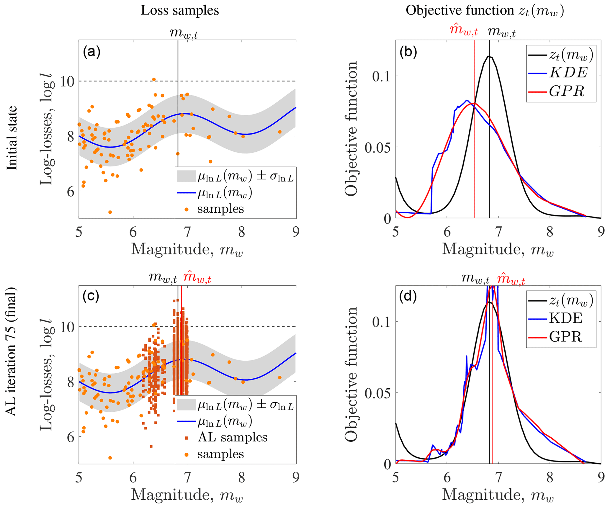
Figure 3Illustration of active learning (AL) for maximizing the objective function zt(mw) with the fixed value lt, marked with a dashed line in the plots in the left panel (a, c). The solution mw,t is approximated with the sample point . The loss samples before and during the AL steps are shown in the left panel (b, d). The approximations of the objective function, either with kernel density estimation (KDE) or Gaussian process regression (GPR), are shown in the right panel (b, d).
4.1 Residential-building stock subjected to a single seismic source with a variable magnitude
Figure 3 illustrates the performance of the acquisition function on a one-dimensional example. In the example, the only source parameter is the magnitude Mw, which follows beta distribution with shape parameters α=1 and β=3 that is scaled between 0 and 10. The conditional distribution of the logarithm of the losses associated with the residential-building stock given Mw=mw is a normal random variable with a mean and standard deviation σln L=0.7. We set lt=10 for this example.
We generate a synthetic earthquake catalog of size n=100. The KDEs are computed with the Gaussian kernel and n2=70 loss samples or more if the scenario has more than n2 conditional-loss evaluations, and the bootstrap standard deviation is computed based on nb=100 samples. We perform the GPR on the whole catalog and learn the hyperparameters at every AL step, since the catalog size in this example is not restrictive. For the AL stage, we select ns=5 scenarios per AL iteration for computing nl=10 loss evaluations at each scenario (i.e., damage evaluations per AL iteration). The acquisition function is the AEI, as introduced in Eq. (21). We also let the algorithm achieve convergence with a maximum of n3=1000 AL iterations, with the convergence criterion in Eq. (25) and r=0.001.
Figure 3 compares intermediate and final results for this example to the true results. After the initial loss evaluations at the 100 scenarios, the estimate of the objective function is poor. However, the acquisition function is able to select scenarios near the true solution. In the final step, one can observe that estimates of the objective function values have high noise, but the GPR is effective in reducing this noise. The resulting estimate of the objective function is close to the true value around the optimum.
4.2 Residential-building stock subjected to an earthquake with an unknown magnitude and location
This simple example is adapted from Rosero-Velásquez and Straub (2022). It considers a hypothetical fault, where strong earthquakes occur with a rate of . We consider the damage that earthquakes cause to a residential-building stock in a small town. The source parameters are the magnitude Mw and the average hypocentral distance R from the earthquake source to the buildings. The source model for Θ (fΘ(θ)) is a normal distribution with a mean vector μΘ and covariance matrix ΣΘ given as follows:
A standard deviation σ represents the uncertainty in the ground motion, damage measure, and losses. The losses L are a log-normal random variable with parameters and . With these choices, the conditional density fΘ|L(θ|lt) can be evaluated analytically. It is a normal distribution, whose mean vector is the representative earthquake scenario for a return period t.
We set σ=0.5 and use return periods of 50, 100, 500, and 1000 years. The resulting exact representative earthquake scenarios with the loss occurrence approach are , , , and . We use them to verify the proposed sampling-based algorithm.
To estimate θt with the proposed methodology, a synthetic earthquake catalog with random scenarios is employed. We simulate the losses once at each scenario, approximate lt, and compute the KDEs at each scenario. The KDEs are based on n2=200 loss values, computed with the Gaussian kernel, and the bootstrap variance is computed with nb=100 repetitions. We perform GPR with a training set of size ntrain=1500, which is constructed as described in Sect. 3.3.
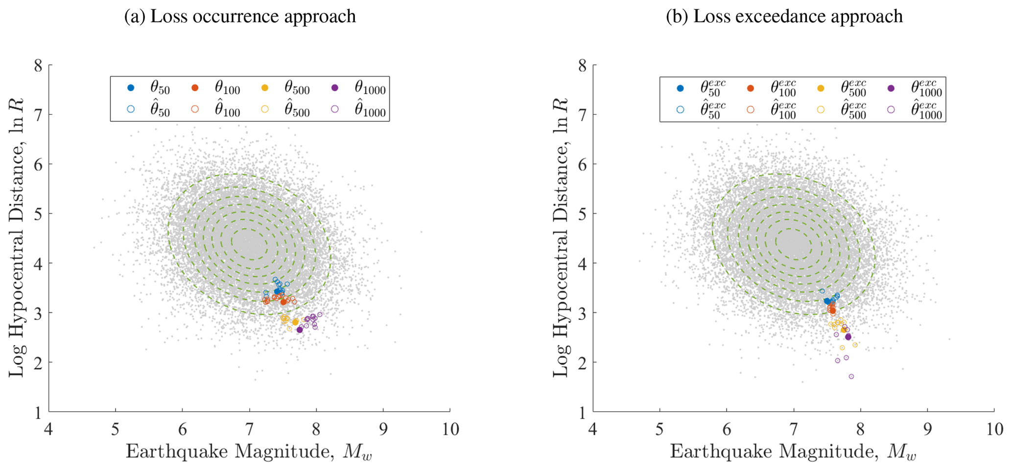
Figure 4Numerical approximation of the representative earthquake scenarios. Panel (a) shows the representative scenarios computed with the loss occurrence approach , and panel (b) shows those computed with the loss exceedance approach . The representative earthquake scenarios correspond to four different return periods, t=50, 100, 500, and 1000 years, based on a Monte Carlo sample of scenarios. Each return period is represented by a different color. For each return period, the 20 approximations of (), corresponding to 20 experiments, are the colored empty circles, and the corresponding exact solutions are depicted by filled circles. The grey points are the scenarios of the catalog, and the dashed contours represent the probability density function (PDF) of the source parameters.
The maximum number of AL iterations is n3=1000, where at every step the losses are evaluated at ns=2 scenarios nl=10 times, for each return period. The procedure stops after the maximum AEI is below ϵ, with r=0.001, for at least nd=5 consecutive AL iterations. For analyzing the uncertainty in the estimation of θt, we repeat the experiment 20 times. For the 50-, 100-, and 500-year representative scenarios, all experiments converged in less than 10 AL iterations, whereas for the 1000-year return period at most 30 AL iterations were required. For the loss exceedance approach, fewer iterations were required in general.
Figure 4 shows the resulting representative hazard scenarios for each return period and their spread, which is mainly caused by the numerical approximation of the objective function with a limited number of samples. As expected, one can observe that the representative scenarios are more extreme when using the loss exceedance approach.
5.1 Context of the study area
We apply the proposed methodology to determine representative earthquake scenarios for the communes of Valparaíso and Viña del Mar, which are located in the Chilean region of Valparaíso on the Pacific coast. The study area is the second-largest Chilean urban center; based on the latest Chilean census (INE, 2017), it is home to 630 903 inhabitants. It hosts the Port of Valparaíso, which is an important container port and the main passenger port in Chile. The area has a heterogeneous building inventory, ranging from apartment buildings to informal settlements and a historic district declared a World Heritage Site by UNESCO in 2003 (Indirli et al., 2011; Jiménez et al., 2018).
The National Electric System (SEN) provides the area's power supply. The SEN is the largest Chilean transmission grid and covers most of the national territory. The SEN connects power plants and substations with the consumer areas through high-voltage lines. The topology of the SEN is characterized as a single-scale network with a fast decaying tail, and most of the load substations are close to a generation unit, with a median distance of 9 km (Ferrario et al., 2022).
Powerful earthquakes have hit the area in the past, such as the 1730 earthquake, with an inferred magnitude Mw in the range of 9.1–9.3, and the 1906 event, with an inferred moment magnitude Mw of 8.0–8.2 (Carvajal et al., 2017). More recently, the 1985 Mw 8.0 event affected around 230 000 dwellings and 1 million people in the regions of Valparaíso, Maule, O'Higgins, and the Santiago Metropolitan Region and caused residential-building losses of about USD 1.4 billion (in 1985 values) (ONEMI, 1985). The most recent Mw 8.8 Maule earthquake (2010) caused severe structural damage in buildings in Viña del Mar, including in buildings retrofitted in 1985 (Jünemann et al., 2015).
Table 1Representative earthquake scenarios for the urban area of Valparaíso selected by Indirli et al. (2011) from historic events. The epicenter location is reported with a map by Indirli et al. (2011), hence their numeric values; the moment magnitude and depth are reproduced here from the earthquake records of the USGS ComCat (Comprehensive Earthquake Catalog) (USGS, 2023). The 1985 Mw 8.0 earthquake event (33°14′ S, 71°51′ W; depth of 33 km) has source parameters similar to those of the 1906 event, while the 2010 earthquake event occurred after the study of Indirli et al. (2011) was submitted for publication. The event dates are in local time. The locations of the epicenters are shown in the map of Fig. 11.
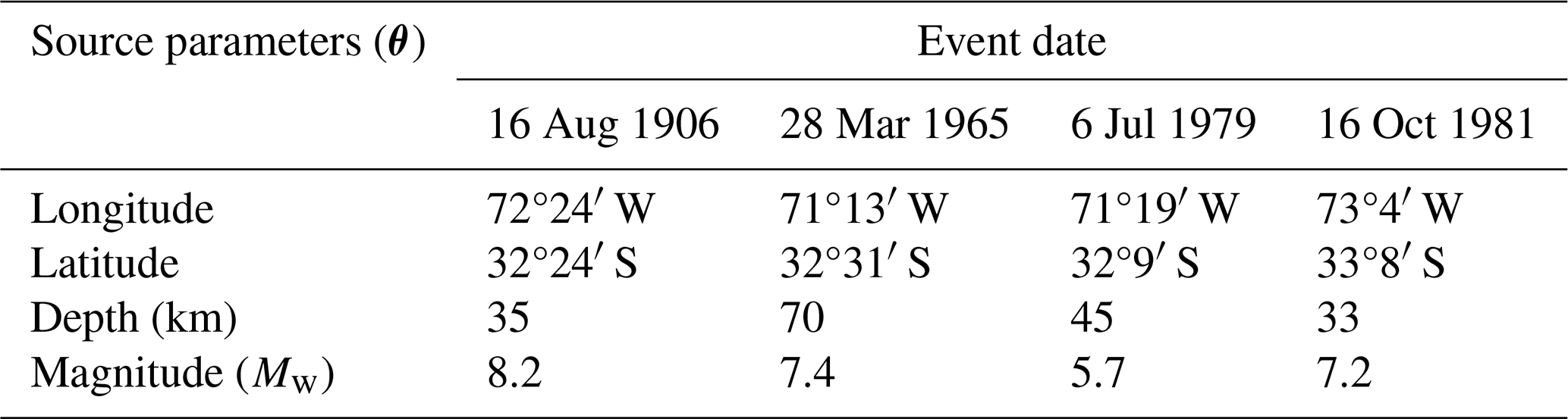
A hazard evaluation of the Valparaíso urban area presented by Indirli et al. (2011) selected representative earthquake scenarios based on historical events, considering the seismicity around the study area, to specify an average regional seismic input and to generate synthetic seismograms. The scenarios are summarized in Table 1; their magnitudes range from Mw=5.7 to Mw=8.2.
5.2 Earthquake model and synthetic earthquake catalog
We employ the earthquake model presented by Poulos et al. (2019) to generate a synthetic catalog of earthquake scenarios. The catalog has 2 × 10⁴ scenarios with a magnitude larger than or equal to Mw=5.0, which is the minimum magnitude defined by Poulos et al. (2019) for performing the declustering on the historical seismic catalogs on which the earthquake model is based on. The catalog covers the whole country of Chile and consists of scenarios at the subduction interface and subduction intraslab zones. The earthquake model utilizes the slab geometry proposed by Hayes et al. (2012) for the depth contours and trench geometry and divides the Chilean subduction zone into three subduction interface and four intraslab zones, whose combined occurrence rate equals λH = 43.3 yr−1.
The epicentral locations of the catalog are generated randomly, based on the occurrence rate associated with the seismic zones defined by the occurrence model. The magnitude is sampled with an importance sampling (IS) approach. We employ a uniform distribution with minimum and maximum values defined by the magnitude range of each seismic zone as the IS density. The corresponding IS weights are considered when determining the loss exceedance function and computed following the original Gutenberg–Richter relationship at each seismic zone (Poulos et al., 2019). The resulting catalog is depicted in Fig. 5, in which one can observe that events of different magnitudes have a similar spread within the seven seismic zones.
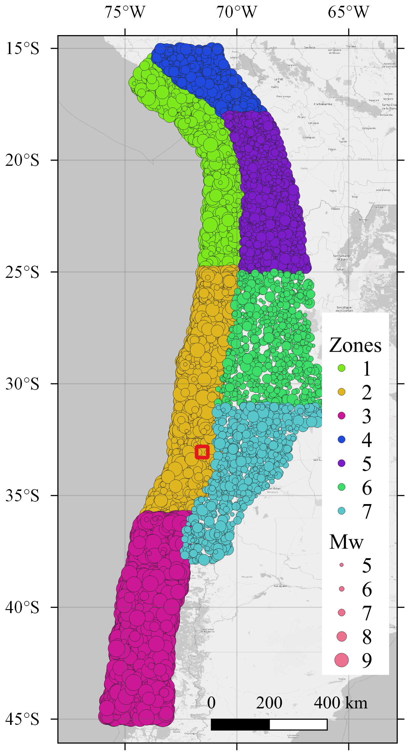
Figure 5Synthetic earthquake catalog with 20 000 scenarios (Poulos et al., 2019). The circle size corresponds to the scenario magnitude. The red square contains the study area. Seismic zones 1 to 3 are of the subduction interface type, and zones 4 to 7 are of the subduction intraslab type. Basemap from © OpenStreetMap contributors 2023. Distributed under the Open Data Commons Open Database License (ODbL) v1.0.
The earthquake model of Poulos et al. (2019) only considers the subduction zone, hence the independent source parameters are the moment magnitude Mw, longitude X, and latitude Y of the epicenter. Other parameters, such as the depth H and the strike, dip, and rake angles, are determined by the geometry derived by Hayes et al. (2012), depending of the epicenter location. Therefore, the PDF of the source parameters fΘ(θ) is represented, respectively, by the conditional PDF and the location-dependent occurrence rate λ(x,y):
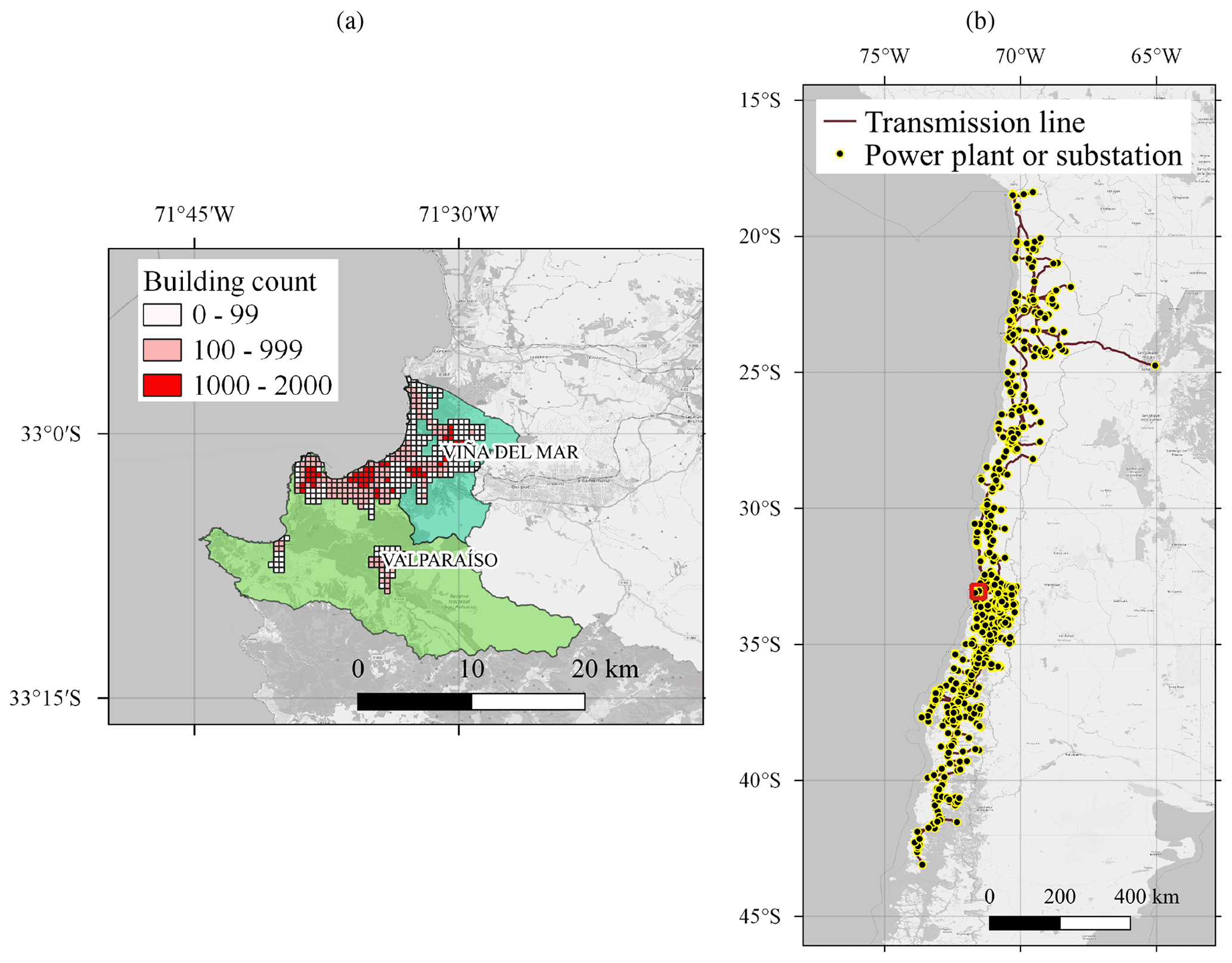
Figure 6(a) Exposure model of the residential-building stock. Each rectangular cell shows the total count of residential buildings, indicating the most dense areas. Source: Pittore et al. (2021). (b) Geographic location of the National Electric System (SEN). The network follows the narrow shape of the country, and the communes of Valparaíso and Viña del Mar (inside red square) are in a central location within the network. Source: Coordinador Eléctrico Nacional (2024), version 2019. Basemap from © OpenStreetMap contributors 2023. Distributed under the Open Data Commons Open Database License (ODbL) v1.0.
5.2.1 Ground motion models
For the residential-building stock, we evaluate the PGA and spectral accelerations at 0.3 and 1.0 s with the ground motion model (GMM) presented by Montalva et al. (2017). The uncertainty in the median prediction is modeled with a Gaussian random field, with the spatial correlation model of Jayaram and Baker (2009a). The choice of these models is based on the epistemic uncertainty analysis of different ground motion and correlation models by Gómez-Zapata et al. (2022a), who analyzed the same study area. For the scope of this study, we do not consider cross-correlated ground motion fields.
For the Chilean power network, we employ the GMM of Abrahamson et al. (2016) and the spatial correlation model developed by Goda and Atkinson (2010) for predicting the PGA. This is the same ground motion model as the one utilized by Ferrario et al. (2022).
The functional form of both GMMs is similar, and therefore, their predictions do not differ significantly, as observed in previous studies (e.g., Hussain et al., 2020; Gómez-Zapata et al., 2022a). In particular, Hussain et al. (2020) found negligible differences in direct loss estimates for the residential-building stock of Santiago de Chile after using these two GMMs to simulate the associated ground motion from subduction earthquake scenarios.
5.3 Model for the residential-building stock in the communes of Valparaíso and Viña del Mar
We employ the Bayesian exposure model of the building stock with the building classes described in Gómez-Zapata et al. (2022a) and available in Pittore et al. (2021). The model was constructed by taking the OpenStreetMap footprint of the buildings in the two communes and assigning to each footprint the most likely building class. The buildings are counted within a regular 500 m × 500 m resolution grid in the urban areas, as shown in Fig. 6. Detailed building counts for each class are presented in Gómez-Zapata et al. (2022a)
The model considers 16 building classes (Gómez-Zapata et al., 2022a) which correspond to the ones proposed in the SARA project (Yepes-Estrada et al., 2017) and have an associated replacement cost. Furthermore, each building class has an associated fragility model with five damage states (Villar-Vega et al., 2017). The fragility model for each building associates an intensity measure (spectral acceleration at 0.3 and 1.0 s or the PGA) with the probabilities of achieving a damage state. We assume the following relative replacement cost percentages for each damage level: 0 % for no damage, 2 % for slight damage, 10 % for moderate damage, 50 % for extensive, and 100 % for complete damage.
We utilize the model to evaluate the ground motion and simulate the building damage. Given an intensity level of the ground motion, the damage is simulated randomly at each building with a discrete distribution with probabilities defined by the fragility functions. The losses for each scenario in the catalog are computed as the accumulated reconstruction cost of the damaged residential buildings, based on the simulated damage.
5.4 Model for the Chilean National Electric System (SEN)
We model the SEN and its components following Ferrario et al. (2022). The network model consists of 1494 nodes, representing 500 generation units and 994 substations, as well as the transmission lines connecting them, with a total power generation capacity of 21.9 GW. The model considers seismic interaction and system performance subjected to component failures. Given a scenario with a ground motion field (in this case, the PGA), each node is randomly associated with a damage state, by means of the fragility function, and a recovery time associated with their damage state.
The losses associated with the SEN due to an earthquake scenario are quantified in terms of the energy not supplied (ENS). The ENS is evaluated at each substation by solving the power in normal steady-state operation through the direct current optimal power flow (DCOPF) model (Wood et al., 2013) and comparing it with the power in a damaged state operation caused by the earthquake scenario. To quantify the loss in the power supply in the communes of Valparaíso and Viña del Mar, we calculate the total ENS with the sum of the ENS of all substations located in the two communes (14 in total).
DCOPF is typically adopted in practice for transmission networks (Frank and Rebennack, 2016). It optimizes the power generation cost, taking into account the capacity of the power plants and transmission lines connected to the power grid, the generation cost associated with each power plant, and the demand from the clients. For modeling the system response to an earthquake, the DCOPF model considers the reduced capacity of components affected by the earthquake. A detailed description and validation of the network model of the SEN can be found in Ferrario et al. (2022).
6.1 Results for the residential-building stock
Figure 7 shows the annual exceedance rate of the losses (in 2016 USD), based on the replacement costs estimated by Yepes-Estrada et al. (2017). The USGS ComCat records that between 1960 and 2020 there were 12 seismic events that produced a macroseismic intensity greater or equal than VI on the Mercalli scale in the two communes (USGS, 2023). This corresponds to an occurrence rate of 0.20 yr−1. It is reasonable to assume that events with a macroseismic intensity of VI or higher lead to losses of at least USD 10 million. For comparison, the reparation cost of the residential buildings in the two communes due to the 1985 earthquake event was USD 49.7 million (in 1985, which corresponds to USD 110.9 million in 2016) (ODEPLAN, 1985). These data therefore validate the lower end of the loss exceedance rate obtained with the synthetic earthquake catalog.
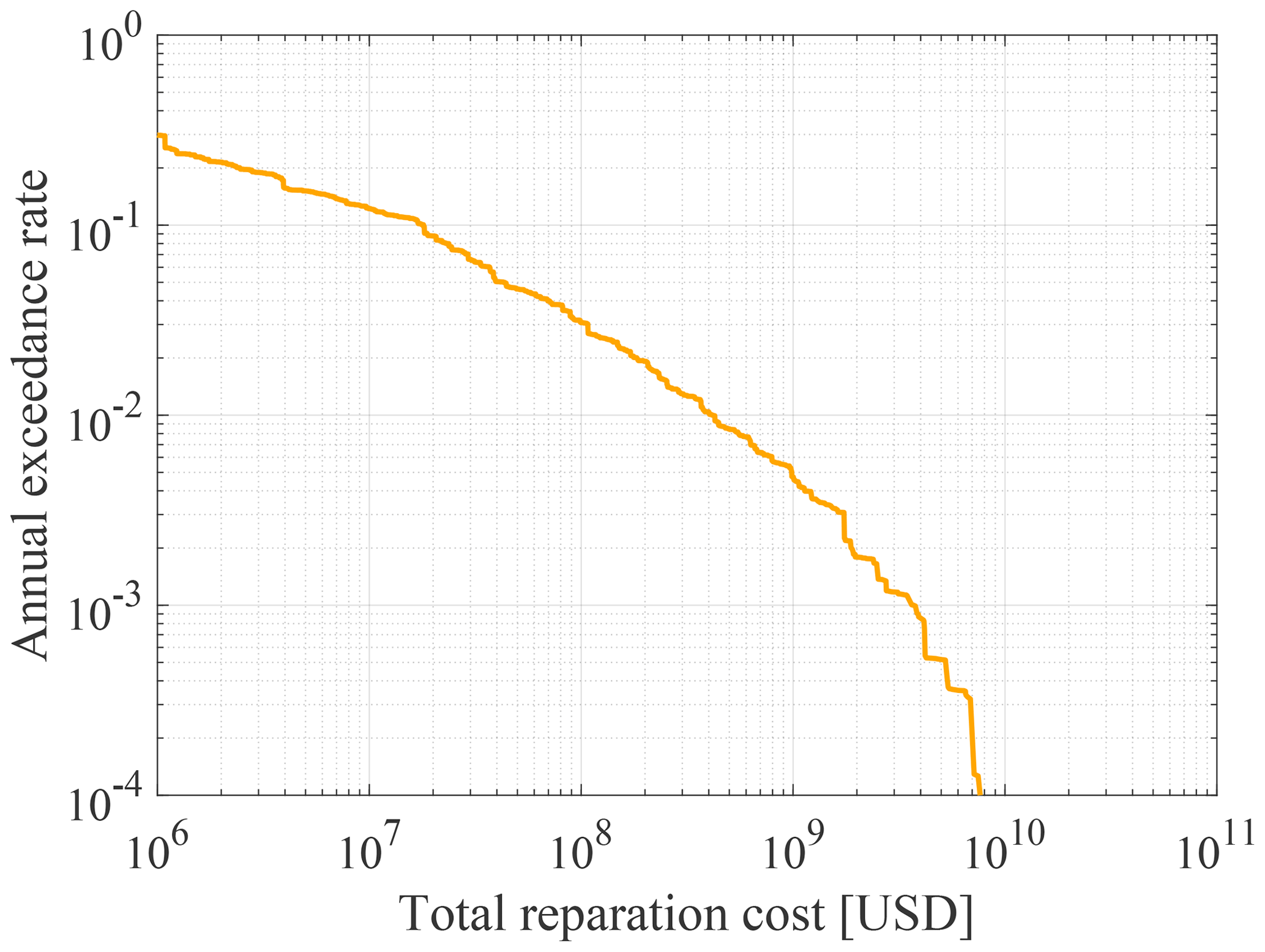
Figure 7Loss exceedance function of the reparation costs (USD in 2016 values) associated with the residential-building stock in the communes of Valparaíso y Viña del Mar.
As in Sect. 4.2, we evaluate the representative scenarios in 20 independent runs of the algorithm to check the robustness of the results. In all evaluations, we found a spread of the identified representative scenarios similar to that of Fig. 4. This spread is larger for higher return periods, but most of the numerical solutions (11 out of 20 for the 1000-year loss return period and at least 16 out of 20 for the other loss return periods) have an epicentral location within a radius of 50 km around the mode, and the coefficient of variation in the magnitude is below 4 % for all return periods. In the following, we only present the modes, i.e., the representative scenarios that were identified the most frequently in the 20 repetitions.
Figure 8 shows the representative earthquake scenarios for the analyzed return periods with a loss occurrence approach. One can observe that large return periods are associated with scenarios that have a larger magnitude. The fact that the magnitude for the 1000-year scenario equals only Mw=7.01 is a consequence of the size of the study area. On the one hand, among the 36 seismic events with Mw≥8.0 registered along the Chilean coast between 1570 and 2023 (CSN, 2023), only 4 events had an epicenter near the two communes, i.e., within a radius of approximately 70 km. For comparison, the identified 1000-year scenario is at a distance of around 20 km from Valparaíso and Viña del Mar. On the other hand, the spatial correlation of the ground motion within a small study area leads to an increased likelihood of extreme losses in a scenario with a lower earthquake magnitude and extreme ground motion residuals. This tendency was also found by Goda and Hong (2009) with the loss exceedance approach.
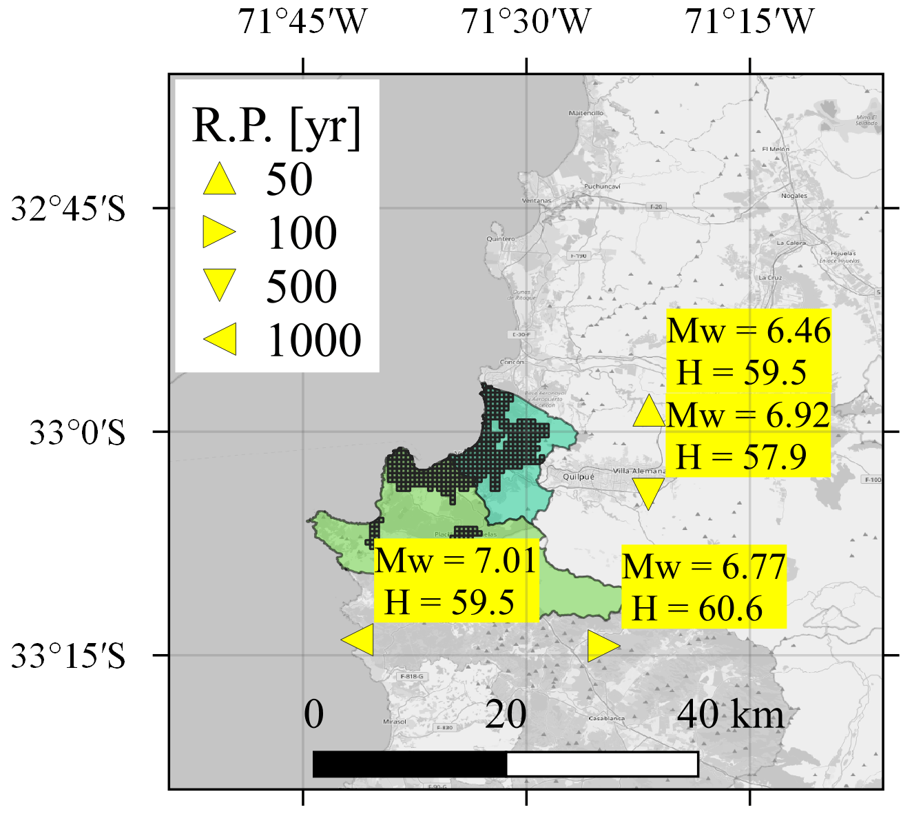
Figure 8Representative earthquake scenarios for the residential-building stock in the communes of Valparaíso and Viña del Mar for four different return periods (RPs). The hypocentral depth H is displayed in kilometers. Source of the exposure model: Pittore et al. (2021). Basemap from © OpenStreetMap contributors 2023. Distributed under the Open Data Commons Open Database License (ODbL) v1.0.
6.2 Results for the power network
Figure 9 shows the loss exceedance function in terms of the ENS obtained with the synthetic earthquake catalog. The largest sampled ENS value is around 2 × 10⁵ MW h, which is around 20 % of the annual energy demand of the two communes.
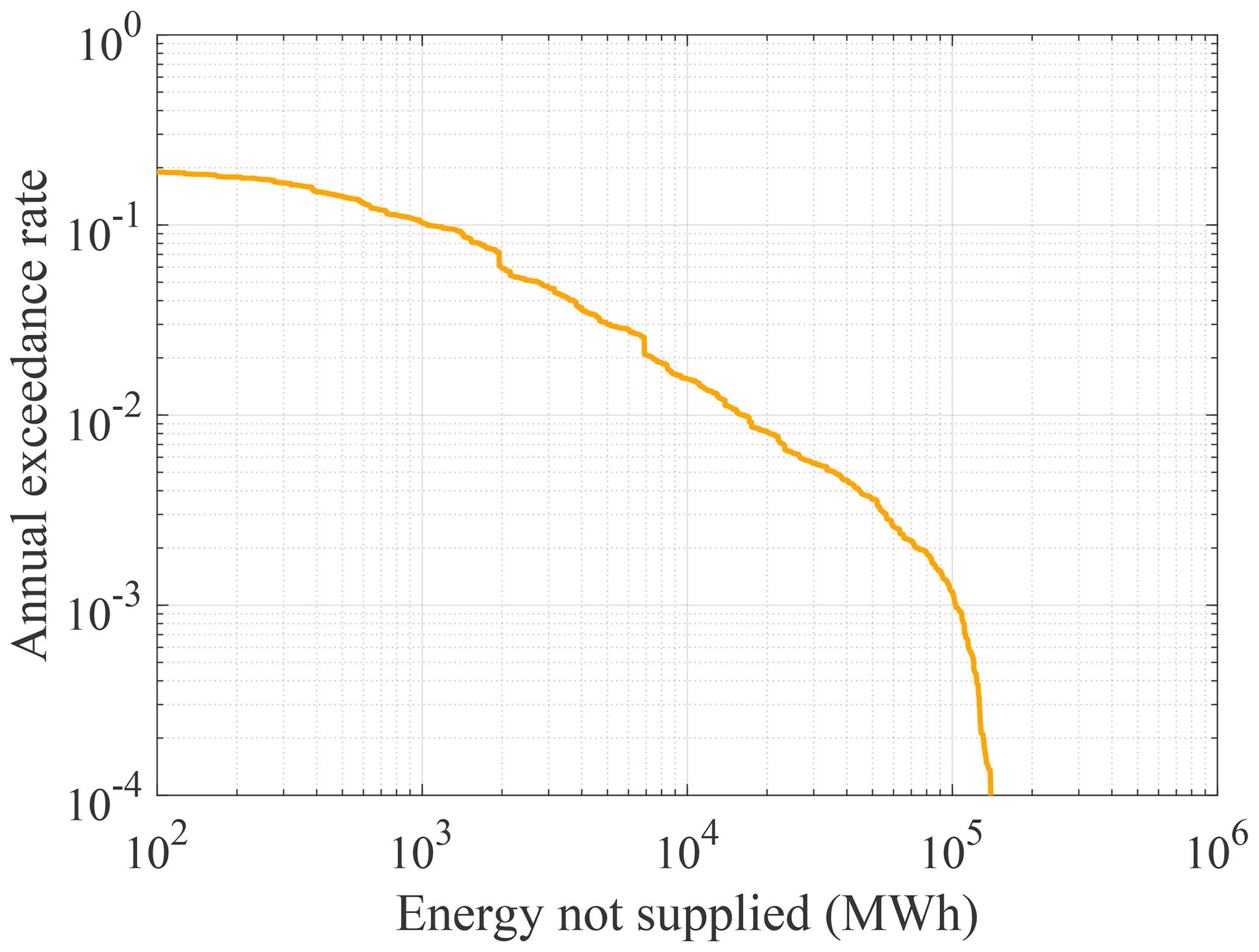
Figure 9Loss exceedance function of the total energy in megawatt hours (MW h) not supplied in communes of Valparaíso and Viña del Mar.
The spread in epicentral locations of the representative scenarios obtained with the 20 runs is larger than the one of the residential-building stock but is still small. At least 13 solutions cluster around the sample mode within a radius of 100 km, and the coefficient of variation in the magnitude is below 5 % for all return periods.
Figure 10 shows the resulting representative earthquake scenarios for the analyzed return periods. One can observe that the scenarios are close to the two communes but less concentrated than those of the residential-building stock and have a different magnitude range. This reflects the fact that the total ENS, although computed only at the substations located within the two communes, depends on the damage state of the components of the rest of network.
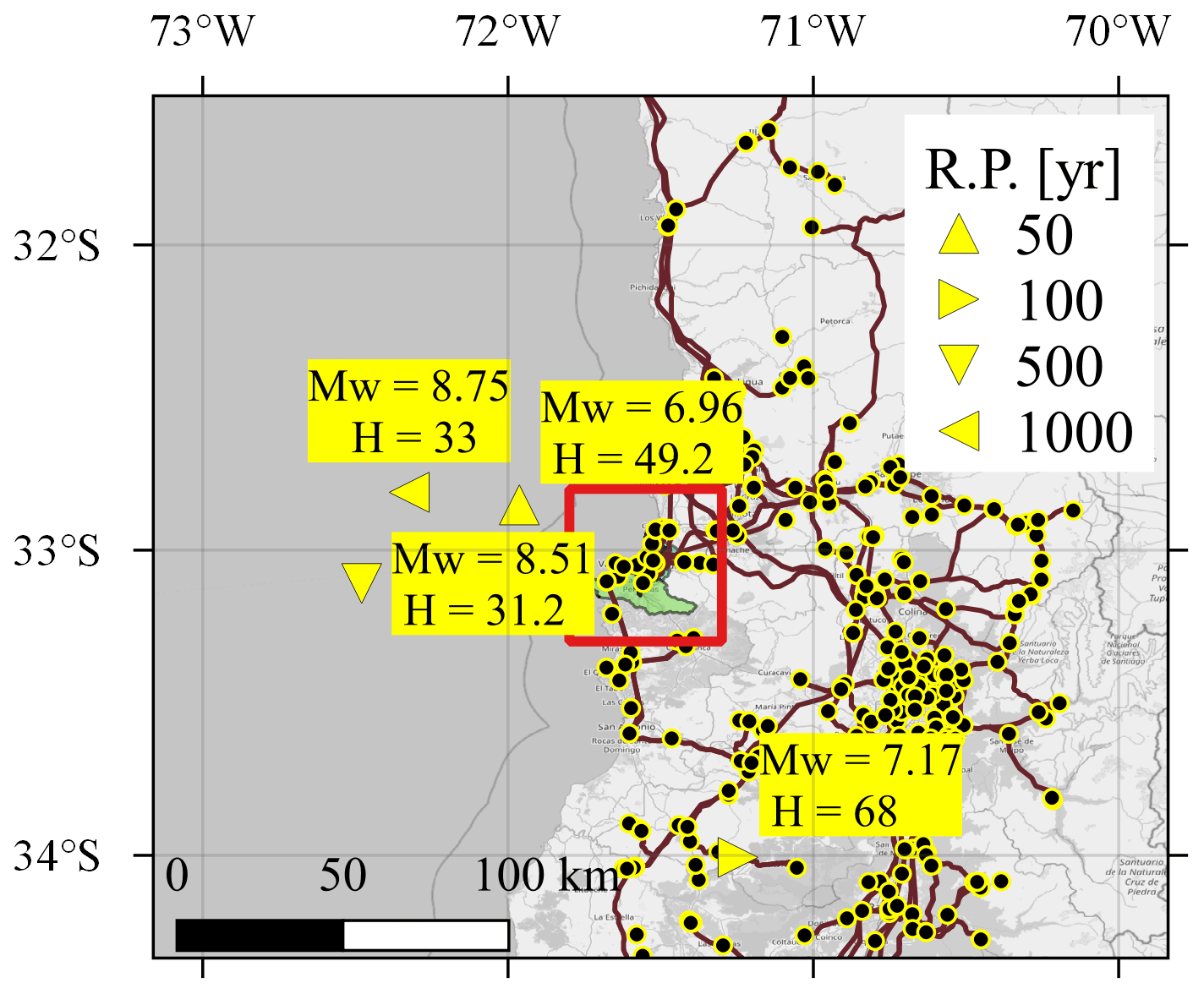
Figure 10Representative earthquake scenarios for the power supply considering the total energy not supplied (ENS) of the communes of Valparaíso and Viña del Mar for four different return periods (RPs). The red square indicates the location of the two communes, and the hypocentral depth H is displayed in kilometers. Source of the power network: Coordinador Eléctrico Nacional (2024). Basemap from © OpenStreetMap contributors 2023. Distributed under the Open Data Commons Open Database License (ODbL) v1.0.
Even though the power supply network is spread out over a larger area, the representative earthquake scenarios are close to the study area. They reflect that the most important components of the network for the two communes are in their proximity. For example, the source location of the 100-year return period scenario lies near a main connection between the substations in the two communes and the rest of the SEN.
6.3 Comparison with past earthquake events
Figure 11 compares the results with the historical events selected in Indirli et al. (2011). Although the representative earthquake scenarios and the selected historical events target the same area of interest, they have different purposes. The historical events presented by Indirli et al. (2011) aim at representing the seismicity of the most important seismic zones affecting the study area. In contrast, the representative earthquake scenarios, as defined in Rosero-Velásquez and Straub (2022), take into account the performance and the losses caused by damage and failures in the analyzed engineering system. In addition, the scenarios are selected based on different loss levels, which are attached to return periods.
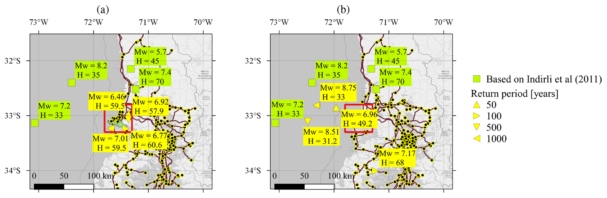
Figure 11Representative earthquake scenarios for the (a) building stock and (b) power supply, compared with past earthquake events selected in Indirli et al. (2011). The location of the two communes is within the red square, and the National Electric System (SEN) network is also displayed. Source of the exposure model: Pittore et al. (2021). Source of the power network: Coordinador Eléctrico Nacional (2024). Basemap from © OpenStreetMap contributors 2023. Distributed under the Open Data Commons Open Database License (ODbL) v1.0.
6.4 Computational cost
In terms of loss evaluations, the analysis requires one evaluation per scenario in the catalog for constructing the loss exceedance function with event-based earthquake risk assessment. That corresponds to 2 × 10⁴ loss evaluations. In addition, during the AL stage, around 10 iterations were necessary to achieve the convergence criterion of Eq. (25), each of them consisting of 160 new loss evaluations (ns=2 scenarios evaluated nl=20 times, for each of the nt=4 return periods). Therefore, 1600 loss evaluations are needed to find the representative earthquake scenarios for four different return periods.
For comparison, Goda and Hong (2009) report that they use a total of 5 × 10⁶ loss evaluations for the classical loss disaggregation. Furthermore, they only evaluate the scenarios with the loss exceedance approach. Extending the loss disaggregation approach to loss occurrence will likely require additional evaluations. Additionally, the computation cost of the loss disaggregation approach scales exponentially with the number of parameters describing seismic scenarios. Hence, the classical loss disaggregation approach will not be applicable to problems in which earthquake scenarios are described by more than three or four parameters. By contrast, we successfully tested the proposed approach for seismic hazard models with seven parameters in applications not reported in this paper.
7.1 On the results for the communes of Valparaíso and Viña del Mar
The representative earthquake scenarios summarized in Fig. 11 can provide important input to risk assessment and risk management activities. The fact that the scenarios identified with the proposed approach differ from the historical events selected in Indirli et al. (2011) should not be surprising, as the latter are in some sense just “random samples” of earthquake events. Nevertheless, the historic events can provide a useful validation of the identified scenarios. In this regard, the scenarios identified as representative of the power supply network appear to be in line with the historic events. The identified 500- and 1000-year scenarios have larger magnitudes than the historical events, which is expected since the historical events come from a (roughly) 100-year period, as shown in Table 1. By contrast, the representative scenarios identified for the building stock have smaller magnitudes than the historical events. However, they occur much closer to the considered building stock. Furthermore, according to the employed model, extreme losses are more likely to occur through a combination of a less strong earthquake with larger-than-average ground motions (i.e., a large value of the interevent term in the GMM). This effect occurs for the residential-building stock due to its spatial concentration and not (or to a much smaller extent) for the power supply network, which is spatially distributed.
The above observations lead to some important conclusions: firstly, the scenarios, rightly, are different for different assets. Secondly, the scenarios depend on model assumptions beyond the seismic source models. In the application here, the model of the ground motion variability has a distinct effect on the scenarios for the residential-building stock. Given that the employed state-of-the-art model might overestimate the event-to-event variability (Bodenmann et al., 2023), the results for the building stock should be utilized carefully. Thirdly, because the earthquake scenario in the building case is representative of certain loss return periods only in combination with high ground motions, it should be investigated if and how the representative scenario should also provide ground motion fields together with the earthquake event. We note that these issues are also present for the classical hazard and loss disaggregation methods. Overall, for practical risk management tasks it is recommended to use the historic events jointly with the identified scenarios, in particular for the residential-building stock case.
The dependence of the results on the engineering system and the model assumptions implies that the representative scenarios should be regularly updated, depending on how much the analyzed system changes and the models improve. According to demographic projections of the Chilean National Statistics Institute (INE), based on the 2017 Chilean census, the population in the two communes will increase by around 13 % by 2035 with respect to the population in 2017 (INE, 2017). This demographical change will likely cause changes in the residential-building stock and the power demand. Depending on how these changes develop, the representative earthquake scenarios may change as well. Furthermore, the presented results do not consider the potential impact caused by further earthquake-triggered hazards, such as tsunamis and landslides. The tsunami impact during offshore earthquake scenarios with a large magnitude should be considered in a complete loss estimation and may affect the scenario selection associated with large return periods. Similarly, the scenario selection may change if one considers the landslides potential in the study area. Finally, cascading effects have not been considered in the power network model. Although the topology of the SEN and the redundancy of generators along the network reduce the probability of large blackouts, hub nodes far from the two communes may affect them through a sequence of failures triggered by earthquake scenarios impacting them. This may shift the representative scenarios to locations further from the study area.
7.2 On the definition of representative scenarios and the methodology for identifying them
We presented the evaluation of representative earthquake scenarios based on the loss occurrence and the loss exceedance approach; the latter coincides with the classical loss disaggregation method (Goda and Hong, 2009; Jayaram and Baker, 2009b). In the illustrative example of Sect. 4.2, we compare the results of the two approaches. For the case of hazard disaggregation, it has been proposed in the literature that the results of both approaches should be reported (Fox, 2023). However, we decided against reporting the scenarios of the exceedance approach for the communes of Valparaíso and Viña del Mar to avoid confusion. We find the loss occurrence approach to have a more intuitive interpretation. Scenarios identified with this approach correspond to a loss that is the t-year loss, which can be reported jointly with the scenarios. They are the most likely scenarios leading to this value (which on average is exceeded once in t years). By contrast, we find it difficult to communicate the meaning of the scenarios with the loss exceedance approach – and we believe it will be mostly misunderstood. Scenarios obtained with the loss occurrence approach can be described as “representative of a loss that is exceeded on average once in t years”. For the loss exceedance approach, one would need to describe scenarios as “representative of the losses that would occur when conditioning on a loss at least as large as the one that would be exceeded once in t years”, which seems too convoluted to communicate effectively. We also have difficulties in conceiving of a risk management activity for which such a definition would be more appropriate. However, we acknowledge that this discussion could benefit from additional comparisons of the two approaches in future studies.
To evaluate the representative scenarios, we adapted the methodology of Rosero-Velásquez and Straub (2022). The methodology leads to a lower computational cost in terms of loss evaluations compared to the classical loss disaggregation. By incorporating active learning, the methodology concentrates the conditional-loss evaluations around the scenarios that most likely produce the t-year loss value lt. This concentration of samples around the solution and the smooth approximation of the conditional density with KDE make the methodology more suitable for selecting representative scenarios with the loss occurrence approach. For this approach, the classical loss disaggregation has to rely on the numerical derivative of the empirical CDF (Baker et al., 2021).
Although single representative scenarios are valuable for risk mitigation and communication purposes, they also have several limitations. For example, designing effective risk mitigation strategies, such as resource allocation before the event, using a single representative scenario would result in solutions tailored to the spatial distribution of damage of the specific selected scenario. Thus, better strategies could be defined by considering multiple scenarios, even for the same loss return period.
Possible extensions of the methodology include catalogs with multiple hazards (e.g., seismic scenarios with a tsunami), loss calculations considering indirect consequences, and high-dimensional scenarios (e.g., including the damage states of the individual components, either buildings or power network components). For the later, however, the dimensionality of the damage states has to be reduced (Rosero-Velásquez and Straub, 2019).
We present a methodology and algorithm to determine representative earthquake scenarios from a synthetic earthquake catalog. We applied the methodology to the communes of Valparaíso and Viña del Mar in Chile. Because the identified scenarios should be representative of extreme losses, they differ depending on the exposed assets. In this contribution, we consider the building stock and the electrical supply network. The application shows that the methodology can work and allows for the identification of scenarios more systematically than by selection or extrapolation from past events. However, the results for the residential-building stock also show that resulting scenarios cannot be considered independently of the resulting ground motions. Therefore, future work should investigate scenarios that also include the ground motions. Because the description of ground motion fields requires a large number of parameters, the existing methodology will need to be extended to be able to cope with such scenarios.
| Acronym | Name |
| PGA | Peak ground acceleration |
| Probability density function | |
| PSHA | Probabilistic seismic hazard analysis |
| GMM | Ground motion model |
| CDF | Cumulative distribution function |
| KDE | Kernel density estimation |
| GPR | Gaussian process regression |
| AL | Active learning |
| AEI | Augmented expected improvement |
| INE | Chilean National Statistics Institute |
| UNESCO | United Nations Educational, Scientific andCultural Organization |
| SEN | Chilean National Electric System |
| ONEMI | Chilean National Office of Emergency ofthe Ministry of the Interior and Public Security |
| USGS | United States Geological Survey |
| IS | Importance sampling |
| SARA | Project “South America Risk Assessment” |
| ENS | Energy not supplied |
| DCOPF | Direct current optimal power flow |
| USD | United States dollar |
| RP | Return period |
| ODEPLAN | Chilean National Planning Office |
| CSN | National Seismological Center of theUniversity of Chile |
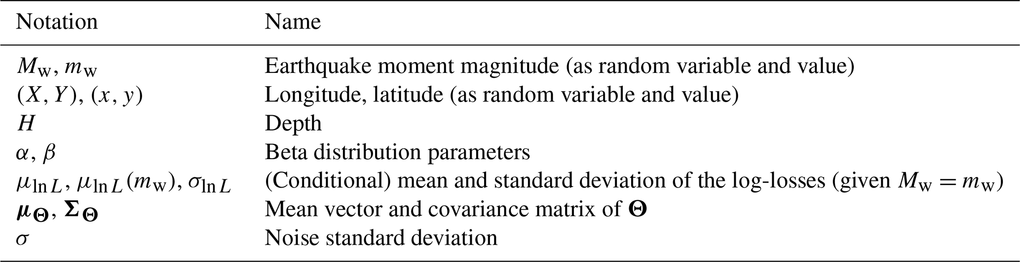
Table B1List of random variables used in this paper, distinguishing the random variable notation from a value and a sample value.
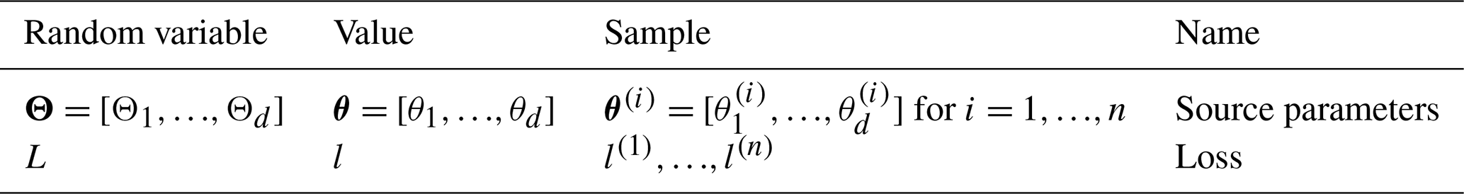
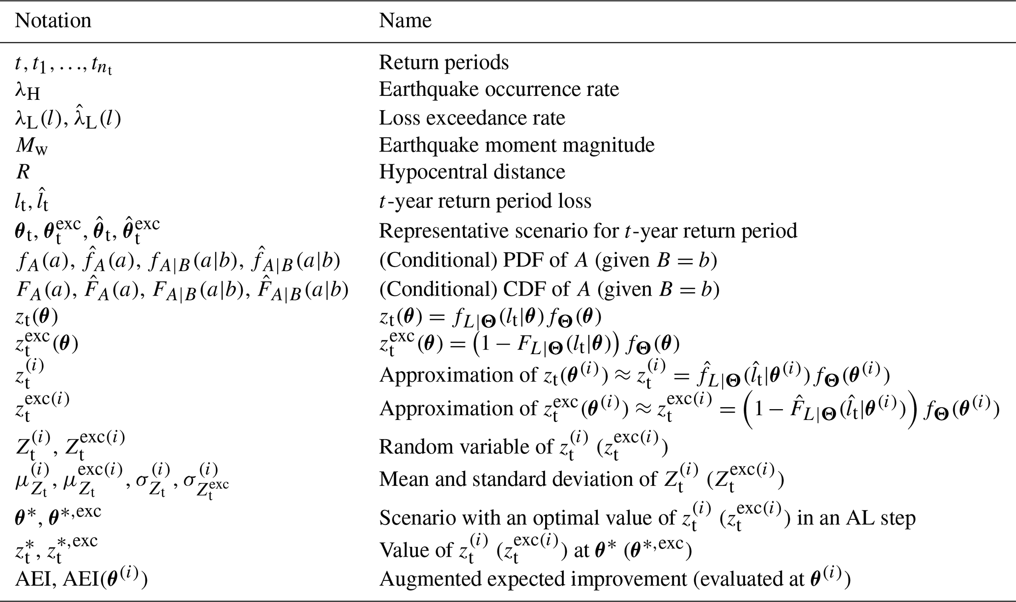
Table B4List of variables and functions used in this paper. Variables with a hat (e.g., ) represent approximations of their respective variables without a hat (e.g., lt). Variables with the superscript exc refer to the exceedance approach, and the corresponding variables without this superscript correspond to the occurrence approach.
The code for scenario selection is available from the authors upon reasonable request. The USGS ComCat is accessible on the USGS website (https://doi.org/10.5066/F7MS3QZH, USGS, 2017.). The database of historic earthquakes is accessible on the website of the National Seismological Center of the University of Chile (CSN) (https://www.sismologia.cl/informacion/grandes-terremotos.html, CSN, 2023). The 2017 Chilean census, organized by the Chilean National Statistics Institute (INE), is available online (http://www.censo2017.cl/servicio-de-mapas, INE, 2017). Technical information about the SEN, the Chilean power transmission network, is accessible through the Infotecnica website from the National Electrical Coordinator (https://infotecnica.coordinador.cl/, Coordinador Eléctrico Nacional, 2024).
This paper was conceptualized by HRV and DS. The methodology was developed by HRV and DS. The investigation for the hazard modeling (i.e., source model, seismic catalog) was conducted by AP, JCGZ, JCL, HRV, and DS. The investigation for the power supply application (i.e., network model and numerical simulations) was conducted by MM, EF, JCL, and HRV. The investigation for the residential-building stock (i.e., exposure and vulnerability model and numerical simulations) was conducted by JCGZ and HRV. Visualizations were completed by HRV, and the interpretation was performed by HRV and DS. The original draft was prepared by HRV, MM, and DS. The paper was reviewed and edited by HRV, AP, JCGZ, JCL, MM, EF, and DS. Funding acquisition for this work was done by DS and JCL.
The contact author has declared that none of the authors has any competing interests.
Publisher's note: Copernicus Publications remains neutral with regard to jurisdictional claims made in the text, published maps, institutional affiliations, or any other geographical representation in this paper. While Copernicus Publications makes every effort to include appropriate place names, the final responsibility lies with the authors.
This article is part of the special issue “Multi-risk assessment in the Andes region”. It is not associated with a conference.
This work has been sponsored by the research and development project RIESGOS 2.0 (grant no. 03G0905A-H), funded by the German Federal Ministry of Education and Research (BMBF) as part of the funding program BMBF CLIENT II – International Partnerships for Sustainable Innovations and by the Chilean government through the Research Center for Integrated Disaster Risk Management (CIGIDEN; grant no. ANID/FONDAP/1523A0009) and the research project Multiscale earthquake risk mitigation of healthcare networks using seismic isolation (grant no. ANID/FONDECYT/1220292). We also thank Fabrice Cotton (GFZ) for his support during the production of this study.
This research has been supported by the Bundesministerium für Bildung und Forschung (grant no. 03G0905A-H) and the Agencia Nacional de Investigación y Desarrollo (grant nos. ANID/FONDAP/1523A0009 and ANID/FONDECYT/1220292).
This paper was edited by Elisabeth Schoepfer and reviewed by two anonymous referees.
Abrahamson, N., Gregor, N., and Addo, K.: BC hydro ground motion prediction equations for subduction earthquakes, Earthq. Spectra, 32, 23–44, https://doi.org/10.1193/051712EQS188MR, 2016. a
Aguirre, P., Vásquez, J., de la Llera, J. C., González, J., and González, G.: Earthquake damage assessment for deterministic scenarios in Iquique, Chile, Nat. Hazards, 92, 1433–1461, https://doi.org/10.1007/s11069-018-3258-3, 2018. a, b
Allen, E., Chamorro, A., Poulos, A., Castro, S., de la Llera, J. C., and Echaveguren, T.: Sensitivity analysis and uncertainty quantification of a seismic risk model for road networks, Comput.-Aided Civ. Inf., 37, 516–530, https://doi.org/10.1111/mice.12748, 2022. a, b
Baker, J., Bradley, B., and Stafford, P.: Seismic Hazard and Risk Analysis, Cambridge University Press, Cambridge, UK, https://doi.org/10.1017/9781108425056, 2021. a, b
Bazzurro, P. and Cornell, C. A.: Disaggregation of seismic hazard, B. Seismol. Soc. Am., 89, 501–520, https://doi.org/10.1785/BSSA0890020501, 1999. a
Bodenmann, L., Baker, J. W., and Stojadinović, B.: Accounting for path and site effects in spatial ground-motion correlation models using Bayesian inference, Nat. Hazards Earth Syst. Sci., 23, 2387–2402, https://doi.org/10.5194/nhess-23-2387-2023, 2023. a
Borzoo, S., Bastami, M., and Fallah, A.: Extreme scenarios selection for seismic assessment of expanded lifeline networks, Struct. Infrastruct. E., 17, 1386–1403, https://doi.org/10.1080/15732479.2020.1811989, 2021. a
Candia, G., Poulos, A., de la Llera, J. C., Crempien, J. G., and Macedo, J.: Correlations of spectral accelerations in the Chilean subduction zone, Earthq. Spectra, 36, 788–805, https://doi.org/10.1177/8755293019891723, 2020. a
Carvajal, M., Cisternas, M., and Catalán, P. A.: Source of the 1730 Chilean earthquake from historical records: Implications for the future tsunami hazard on the coast of Metropolitan Chile, J. Geophys. Res.-Sol. Ea., 122, 3648–3660, https://doi.org/10.1002/2017JB014063, 2017. a, b
Chatelain, J.-L., Yepes, H., Bustamante, G., Fernández, J., Valverde, J., Kaneko, F., Villacis, C., Yamada, T., and Tucker, B.: Proyecto para Manejo del Riesgo sísmico de Quito, Escuela Politécnica Nacional, Quito, Ecuador, 1995. a
Coordinador Eléctrico Nacional: Infotécnica Sistema Eléctrico Nacional, https://infotecnica.coordinador.cl/ (last access: February 2024), 2024. a, b, c, d
Cornell, C. A.: Engineering seismic risk analysis, B. Seismol. Soc. Am., 58, 1583–1606, 1968. a
CSN: Grandes terremotos en Chile, CSN [data set], https://www.sismologia.cl/informacion/grandes-terremotos.html (last access: February 2024), 2023. a, b
de la Llera, J. C., Rivera, F., Mitrani-Reiser, J., Jünemann, R., Fortuño, C., Ríos, M., Hube, M., Santa María, H., and Cienfuegos, R.: Data collection after the 2010 Maule earthquake in Chile, B. Earthquake E., 15, 555–588, https://doi.org/10.1007/s10518-016-9918-3, 2017. a
Efron, B. and Tibshirani, R. J.: An Introduction to the Bootstrap, Chapman & Hall/CRC, Boca Raton, FL, USA, https://doi.org/10.1201/9780429246593, 1993. a
Esteva, L.: Regionalización sísmica de México para fines de ingeniería, Instituto de Ingeniería, UNAM, Mexico, https://aplicaciones.iingen.unam.mx/ConsultasSPII/DetallePublicacion.aspx?id=152 (last access: 18 July 2024), 1970. a
Feliciano, D., Arroyo, O., Cabrera, T., Contreras, D., Valcárcel Torres, J. A., and Gómez Zapata, J. C.: Seismic risk scenarios for the residential buildings in the Sabana Centro province in Colombia, Nat. Hazards Earth Syst. Sci., 23, 1863–1890, https://doi.org/10.5194/nhess-23-1863-2023, 2023. a
Ferrario, E., Poulos, A., Castro, S., de la Llera, J., and Lorca, A.: Predictive capacity of topological measures in evaluating seismic risk and resilience of electric power networks, Reliab. Eng. Syst. Safe., 217, 108040, https://doi.org/10.1016/j.ress.2021.108040, 2022. a, b, c, d, e, f
Fox, M.: Considerations on seismic hazard disaggregation in terms of occurrence or exceedance in New Zealand, Bull. N. Z. Soc. Earthq. Eng., 56, 1–10, https://doi.org/10.5459/bnzsee.56.1.1-10, 2023. a, b
Fox, M. J., Stafford, P. J., and Sullivan, T. J.: Seismic hazard disaggregation in performance-based earthquake engineering: occurrence or exceedance?, Earthq. Eng. Struct. D., 45, 835–842, https://doi.org/10.1002/eqe.2675, 2016. a, b
Frank, S. and Rebennack, S.: An introduction to optimal power flow: Theory, formulation, and examples, IIE Trans., 48, 1172–1197, https://doi.org/10.1080/0740817X.2016.1189626, 2016. a
Gisbert, F. J. G.: Weighted samples, kernel density estimators and convergence, Empir. Econ., 28, 335–351, https://doi.org/10.1007/s001810200134, 2003. a
Goda, K. and Atkinson, G. M.: Intraevent spatial correlation of ground-motion parameters using SK-net data, B. Seismol. Soc. Am., 100, 3055–3067, https://doi.org/10.1785/0120100031, 2010. a
Goda, K. and Hong, H. P.: Deaggregation of seismic loss of spatially distributed buildings, B. Earthquake E., 7, 255–272, https://doi.org/10.1007/s10518-008-9093-2, 2009. a, b, c, d, e, f
Gómez-Zapata, J. C., Zafrir, R., Pittore, M., and Merino, Y.: Towards a sensitivity analysis in seismic risk with probabilistic building exposure models: An application in Valparaíso, Chile, using ancillary open-source data and parametric ground motions, ISPRS Int. J. Geo-Inf., 11, 113, https://doi.org/10.3390/ijgi11020113, 2022a. a, b, c, d, e
Gómez-Zapata, J. C., Pittore, M., Cotton, F., Lilienkamp, H., Shinde, S., Aguirre, P., and Santa María, H.: Epistemic uncertainty of probabilistic building exposure compositions in scenario-based earthquake loss models, B. Earthquake E., 20, 2401–2438, https://doi.org/10.1007/s10518-021-01312-9, 2022b. a
Hayes, G. P., Wald, D. J., and Johnson, R. L.: Slab1.0: A three-dimensional model of global subduction zone geometries, J. Geophys. Res.-Sol. Ea., 117, B01302, https://doi.org/10.1029/2011JB008524, 2012. a, b
Huang, D., Allen, T. T., Notz, W. I., and Miller, R. A.: Sequential Kriging optimization using multiple-fidelity evaluations, Struct. Multidiscip. O., 32, 369–382, https://doi.org/10.1007/s00158-005-0587-0, 2006. a, b, c, d, e, f
Hussain, E., Elliott, J. R., Silva, V., Vilar-Vega, M., and Kane, D.: Contrasting seismic risk for Santiago, Chile, from near-field and distant earthquake sources, Nat. Hazards Earth Syst. Sci., 20, 1533–1555, https://doi.org/10.5194/nhess-20-1533-2020, 2020. a, b
Indirli, M., Razafindrakoto, H., Romanelli, F., Puglisi, C., Lanzoni, L., Milani, E., Munari, M., and Apablaza, S.: Hazard evaluation in Valparaíso: the MAR VASTO project, Pure Appl. Geophys., 168, 543–582, https://doi.org/10.1007/s00024-010-0164-3, 2011. a, b, c, d, e, f, g, h, i, j, k, l, m
INE: Servicio de mapas del Censo 2017, http://www.censo2017.cl/servicio-de-mapas (last access: February 2024), 2017. a, b, c
Jayaram, N. and Baker, J. W.: Correlation model for spatially distributed ground-motion intensities, Earthq. Eng. Struct. D., 38, 1687–1708, https://doi.org/10.1002/eqe.922, 2009a. a
Jayaram, N. and Baker, J. W.: Deaggregation of lifeline risk: Insights for choosing deterministic scenario earthquakes, in: Proceedings of the Technical Council on Lifeline Earthquake Engineering Conference, Oakland, California, 28 June–1 July 2009, https://doi.org/10.1061/41050(357)100, 2009b. a, b, c, d, e
Jiménez, B., Pelá, L., and Hurtado, M.: Building survey forms for heterogeneous urban areas in seismically hazardous zones: Application to the historical center of Valparaíso, Chile, Int. J. Archit. Herit., 12, 1076–1111, https://doi.org/10.1080/15583058.2018.1503370, 2018. a, b
Jiménez Martínez, M., Jiménez Martínez, M., and Romero-Jarén, R.: How resilient is the labour market against natural disaster? Evaluating the effects from the 2010 earthquake in Chile, Nat. Hazards, 104, 1481–1533, https://doi.org/10.1007/s11069-020-04229-9, 2020. a
Jünemann, R., de la Llera, J., Hube, M., Cifuentes, L., and Kausel, E.: A statistical analysis of reinforced concrete wall buildings damaged during the 2010, Chile earthquake, Eng. Struct., 82, 168–185, https://doi.org/10.1016/j.engstruct.2014.10.014, 2015. a, b
McGuire, R. K.: Probabilistic seismic hazard analysis and design earthquakes: Closing the loop, B. Seismol. Soc. Am., 85, 1275–1284, https://doi.org/10.1785/BSSA0850051275, 1995. a
Miller, M. and Baker, J.: Ground-motion intensity and damage map selection for probabilistic infrastructure network risk assessment using optimization, Earthq. Eng. Struct. D., 44, 1139–1156, https://doi.org/10.1002/eqe.2506, 2015. a
Montalva, G. A., Bastías, N., and Rodriguez-Marek, A.: Ground motion prediction equation for the Chilean subduction zone, B. Seismol. Soc. Am., 107, 901–911, https://doi.org/10.1785/0120160221, 2017. a, b
ODEPLAN: Plan de reconstrucción: Sismo marzo 1985, Of. de Planificación Nal., Santiago de Chile, https://www.desarrollosocialyfamilia.gob.cl/btca/txtcompleto/DIGITALIZADOS/ODEPLAN/O32Ppr-1985-pdf (last access: 18 July 2024), 1985. a
ONEMI: Informe sobre el terremoto de marzo 1985 en Chile, Of. Nal. de Emergencias del Min. del Interior, Santiago de Chile, https://bibliogrd.senapred.gob.cl/handle/2012/125 (last access: 18 July 2024), 1985. a
Pagani, M., Johnson, K., and Garcia Pelaez, J.: Modelling subduction sources for probabilistic seismic hazard analysis, Geol. Soc. Spec. Publ., 501, 225–244, https://doi.org/10.1144/SP501-2019-120, 2021. a
Pittore, M., Gómez-Zapata, J., Brinckmann, N., and Rüster, M.: Assetmaster and Modelprop: web services to serve building exposure models and fragility functions for physical vulnerability to natural-hazards. V.1.0., GFZ Data Services [code], https://doi.org/10.5880/riesgos.2021.005, 2021. a, b, c, d
Poulos, A., Monsalve, M., Zamora, N., and de la Llera, J. C.: An updated recurrence model for Chilean subduction seismicity and statistical validation of its Poisson nature, B. Seismol. Soc. Am., 109, 66–74, https://doi.org/10.1785/0120170160, 2019. a, b, c, d, e, f, g, h
Rasmussen, C. and Williams, C.: Gaussian Processes for Machine Learning, The MIT Press, Cambridge, MA, USA, https://doi.org/10.7551/mitpress/3206.001.0001, 2005. a, b
Rosero-Velásquez, H. and Straub, D.: Selecting Representative Scenarios for Contingency Analysis of Infrastructure Systems with Dependent Component Failures, in: Proceedings of the 13th International Conference on Applications of Statistics and Probability in Civil Engineering, 26–30 May 2019, Seoul, South Korea, 1–8, https://doi.org/10.22725/ICASP13.335, 2019. a
Rosero-Velásquez, H. and Straub, D.: Selection of representative natural hazard scenarios for engineering systems, Earthq. Eng. Struct. D., 51, 3680–3700, https://doi.org/10.1002/eqe.3743, 2022. a, b, c, d, e, f, g, h, i, j
Salgado-Gálvez, M. A., Zuloaga, D., Henao, S., Bernal, G. A., and Cardona, O. D.: Probabilistic assessment of annual repair rates in pipelines and of direct economic losses in water and sewage networks: application to Manizales, Colombia, Nat. Hazards, 93, 5–24, https://doi.org/10.1007/s11069-017-2987-z, 2018. a, b
Silva, V.: Critical issues in earthquake scenario loss modeling, J. Earthq. Eng., 20, 1322–1341, https://doi.org/10.1080/13632469.2016.1138172, 2016. a
Silverman, B. W.: Density Estimation for Statistics and Data Analysis, Chapman & Hall/CRC, Boca Raton, FL, ISBN 13 9780412246203, ISBN 10 0412246201, 1986. a, b
Tomar, A. and Burton, H. V.: Active learning method for risk assessment of distributed infrastructure systems, Comput.-Aided Civ. Inf., 36, 438–452, https://doi.org/10.1111/mice.12665, 2021. a
USGS – US Geological Survey: Earthquake Hazards Program, Advanced National Seismic System (ANSS) Comprehensive Catalog of Earthquake Events and Products: Various, https://doi.org/10.5066/F7MS3QZH, 2017. a
USGS: ANSS Comprehensive Earthquake Catalog (ComCat), https://earthquake.usgs.gov/data/comcat/ (last access: February 2024), 2023. a, b
Villar-Vega, M., Silva, M., Crowley, H., Yepes, C., Tarque, N., Acevedo, A., Hube, M., Gustavo, C., and Santa María, H.: Development of a fragility model for the residential building stock in South America, Earthq. Spectra, 33, 581–604, https://doi.org/10.1193/010716EQS005M, 2017. a
Wood, A., Wollenberg, B., and Sheblé, G.: Power Generation, Operation, and Control, John Wiley & Sons Ltd, ISBN 9780471790556, 2013. a
Yepes-Estrada, C., Silva, V., Valcárcel, J., Acevedo, A. B., Tarque, N., Hube, M. A., Coronel, G., and María, H. S.: Modeling the residential building inventory in South America for seismic risk assessment, Earthq. Spectra, 33, 299–322, https://doi.org/10.1193/101915eqs155dp, 2017. a, b, c
- Abstract
- Introduction
- Definition of a representative earthquake scenario
- Method for using scenario selection based on a synthetic earthquake catalog
- Illustrative examples
- Case study: the communes of Valparaíso and Viña del Mar
- Evaluation of representative earthquake scenarios for the communes of Valparaíso and Viña del Mar
- Discussion
- Conclusion
- Appendix A: List of acronyms used in this paper
- Appendix B: Variables used in this paper
- Code and data availability
- Author contributions
- Competing interests
- Disclaimer
- Special issue statement
- Acknowledgements
- Financial support
- Review statement
- References