Empirical tsunami fragility modelling for hierarchical damage levels

The present work proposes a simulation-based Bayesian method for parameter estimation and fragility model selection for mutually exclusive and collectively exhaustive (MECE) damage states. This method uses an adaptive Markov chain Monte Carlo simulation (MCMC) based on likelihood estimation using point-wise intensity values. It identifies the simplest model that fits the data best, among the set of viable fragility models considered. The proposed methodology is demonstrated for empirical fragility assessments for two different tsunami events and different classes of buildings with varying numbers of observed damage and flow depth data pairs. As case studies, observed pairs of data for flow depth and the corresponding damage level from the South Pacific tsunami on 29 September 2009 and the Sulawesi–Palu tsunami on 28 September 2018 are used. Damage data related to a total of five different building classes are analysed. It is shown that the proposed methodology is stable and efficient for data sets with a very low number of damage versus intensity data pairs and cases in which observed data are missing for some of the damage levels.

1 Introduction

Fragility models express the probability of exceeding certain damage thresholds for a given level of intensity for a specific class of buildings or infrastructure. Empirical fragility curves are models derived from observed pairs of damage and intensity data for buildings and infrastructure usually collected, acquired and even partially simulated in the aftermath of disastrous events. Some examples of empirical fragility models are seismic fragility (Rota et al., 2009; Rosti et al., 2021), tsunami fragility (Koshimura et al., 2009a; Reese et al., 2011; a comprehensive review can be found in Charvet et al., 2017), flooding fragility (Wing et al., 2020) and debris flow fragility curves (Eidsvig et al., 2014). Empirical fragility modelling is greatly affected by how the damage and intensity parameters are defined. Mutually exclusive and collectively exhaustive (MECE, see next section for the definition) damage states are quite common in the literature as discrete physical damage states. The MECE condition is necessary for damage states in most probabilistic risk formulations, leading to the mean rate of exceeding loss (e.g. Behrens et al., 2021).

Tsunami fragility curves usually employ the tsunami flow depth as the measure of intensity; although different studies also use other measures like current velocity (e.g. De Risi et al., 2017b; Charvet et al., 2015). Charvet et al. (2015) demonstrate that the flow depth may cease to be an appropriate measure of intensity for higher damage states, and other parameters such as the current velocity, debris impact and scour can become increasingly more important. De Risi et al. (2017b) developed bivariate tsunami fragilities, which account for the interaction between the two intensity measures of tsunami flow depth and current velocity.

Early procedures for empirical tsunami fragility curves used data binning to represent the intensity. For example, Koshimura et al. (2009b) binned the observations by the intensity measure, i.e. the flow depth; however, the latest procedures have mostly used point-wise intensity estimates instead.

Fragility curves for MECE damage states are distinguished by their nicely “laminar” shape; in other words, the curves should not intersect. When fitting empirical fragility curves to observed damage data, this condition is not satisfied automatically. For example, fragility curves are usually fitted for individual damage states separately, and they are filtered afterwards to remove the crossing fragility curves (e.g. Miano et al., 2020), or ordered (“parallel”) fragility models are used from the start (Charvet et al., 2014; Lahcene et al., 2021). Charvet et al. (2014) and De Risi (2017a) also used partially ordered models to derive fragility curves for MECE damage states. They used the multinomial probability distribution to model the probability of being in any of MECE damage states based on binned intensity representation. De Risi et al. (2017a) used Bayesian inference to derive the model parameters for an ensemble of fragility curves.

Empirical tsunami fragility curves are usually constructed using generalised linear models based on probit, logit or the complementary loglog link functions (Charvet et al., 2014; Lahcene et al., 2021). As far as the assessment of the goodness of fit, model comparison and selection are concerned, approaches based on the likelihood ratio and Akaike information criterion, (e.g. Charvet et al., 2014; Lahcene et al., 2021) and on k-fold cross validation have also been used (Chua et al., 2021). For estimating confidence intervals for empirical tsunami fragility curves, bootstrap resampling has been commonly used (Charvet et al., 2014; Lahcene et al., 2021; Chua et al., 2021).

The present paper presents a simulation-based Bayesian method for inference and model class selection for the ensemble modelling of the tsunami fragility curves for MECE damage states for a given class of buildings. By fitting the (positive definite) fragility link function to the conditional probability of being in a certain damage state, given that building is not in any of the preceding states, the method ensures that the fragility curves do not cross (i.e. they are “hierarchical” as in De Risi et al., 2017a). The method uses adaptive Markov chain Monte Carlo simulation (MCMC, Beck and Au, 2002), based on likelihood estimation using point-wise intensity values, to infer the ensemble of the fragility model parameters. Alternative link functions are compared based on log evidence, which considers both the average goodness of fit (based on log likelihood) and the model parsimony (based on relative entropy). This way, among the set of viable models considered, it identifies the simplest model that fits the data best. By “simplest model”, we mean the model having maximum relative entropy (measured using the Kullback–Leibler distance; Kullback and Leibler, 1951) with respect to the data. This usually means the model has a small number of parameters.

2 Methodology

2.1 Definitions of intensity and damage parameters

The intensity measure, IM, (or simply “intensity”, e.g. the tsunami flow depth) refers to a parameter used to convey information about an event from the hazard level to the fragility level – it is an intermediate variable. The damage parameter, D, is a discrete random variable, and the vector of damage levels is expressed as $\left\{D_j,j=\mathrm{0}:N_{\mathrm{DS}}\right\}$, where D_j as the jth damage level (threshold) and N_DS as the total number of damage levels considered (depending on the damage scale being used and on the type of hazard, e.g. earthquake, tsunami, debris flow). Normally, D₀ denotes the no-damage threshold, while $D_{N_{\mathrm{DS}}}$ defines the total collapse or being totally washed away. Let us assume that DS_j is the jth damage state defined by the logical statement that the damage D is between the two damage thresholds D_j and D_j+1; i.e. D is equal to or greater than D_j and smaller than D_j+1 as follows (see also Fig. 1 for a graphical representation of the above expressions):

$$\begin{array}{}\text{(1)}& {\text{DS}}_j\equiv (D\ge D_j)\cdot (D<D_{j+\mathrm{1}}),\end{array}$$

where (⋅) denotes the logical product and is read as “AND”. Obviously, for the last damage state, we have DS${}_{N_{\mathrm{DS}}}\equiv D\ge D_{N_{\mathrm{DS}}}$.

Figure 1 Graphical representation of damage levels D_j and damage states DS_j, where $j=\mathrm{0}:N_{\mathrm{DS}}$.

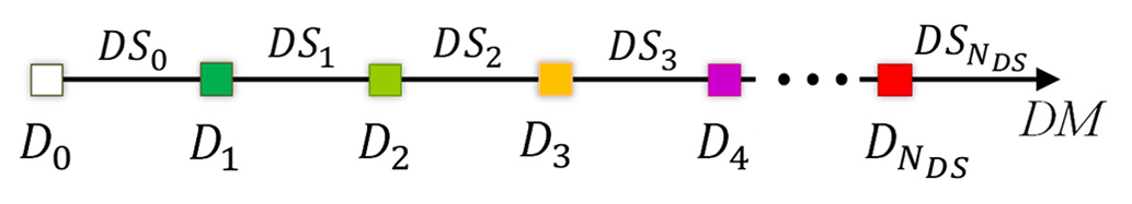
Damage states $\left\{{\text{DS}}_{\mathrm{0}},{\text{DS}}_{\mathrm{1}},\mathrm{\dots },{\text{DS}}_{N_{\mathrm{DS}}}\right\}$ are mutually exclusive and collectively exhaustive (MECE) if and only if $P({\text{DS}}_i\cdot {\text{DS}}_j|\text{IM})=\mathrm{0}$ (if i≠j, $j=\mathrm{0}:N_{\mathrm{DS}}$) and ${\sum }_{j=\mathrm{0}}^{N_{\mathrm{DS}}}P\left({\text{DS}}_j\right|\text{IM})=\mathrm{1}$; (⋅) denotes the logical product and is read as “AND”. In simple words, the damage states are MECE if being in one damage state excludes all others and if all the damage states together cover the entire range of possibilities in terms of damage. The ensemble of MECE damage states DS_j, $j=\mathrm{0}:N_{\mathrm{DS}}$ is usually referred to as the damage scale (e.g. the EMS98; Grünthal, 1998).

The proposed methodology herein is also applicable to fragility assessment in cases where observed damage data are not available for some of the damage levels. Let index be the vector of j values ($j=\mathrm{0}:N_{\mathrm{DS}}$), indicating damage levels N_j for which observed data are available (j values are in ascending order). The new damage scale formed as $\left\{{\text{DS}}_{\mathit{i}\mathit{n}\mathit{d}\mathit{e}\mathit{x}\left(\mathrm{1}\right)},{\text{DS}}_{\mathit{i}\mathit{n}\mathit{d}\mathit{e}\mathit{x}\left(\mathrm{2}\right)},\mathrm{\dots },{\text{DS}}_{\mathit{i}\mathit{n}\mathit{d}\mathit{e}\mathit{x}\left(N\right)}\right\}$ , where N is the length of vector index, is also MECE. It is noteworthy that the number of fragility curves derived in this case is going to be equal to N−1. In the following, for simplicity and without loss of generality, we have assumed that observed data are available for all damage levels, i.e. $\mathit{i}\mathit{n}\mathit{d}\mathit{e}\mathit{x}=\left\{\mathrm{0}:N_{\mathrm{DS}}\right\}$, that is, $N_{\mathrm{DS}}=N-\mathrm{1}$. However, the proposed methodology is also applicable to the modified damage scale formed by damage level indices in vector index(1:N). We will later see examples of such applications in the case studies.

2.2 Fragility modelling using generalised regression models

The generalised regression models (GLMs) are more suitable for empirical fragility assessment with respect to the standard regression models. This is mainly because the dependent variable in the case of the generalised regression models is a Bernoulli binary variable (i.e. only two possible values: 0 or 1). Bernoulli variables are particularly useful in order to detect whether a specific damage level is exceeded or not (only two possibilities). In the following, fragility assessment based on GLMs is briefly described.

The term P(DS_j | IM) denotes the probability of being in damage state DS_j for a given intensity level IM. Based on N_DS damage thresholds, this conditional probability P(DS_j | IM) can be read (see Eq. 1) as the probability that (D≥D_j) and $\left(D<D_{j+\mathrm{1}}\right)$ and can be estimated as follows (see Appendix A for the derivation):

$$\begin{array}{}\text{(2)}& \begin{array}{rl}& P\left({\text{DS}}_j\right|\text{IM})\\ & =P\left[\left(D\ge D_j\right)\cdot \left(D<D_{j+\mathrm{1}}\right)|\text{IM}\right]\\ & =\left\{\begin{array}{l}P(D\ge D_j|\text{IM})-P(D\ge D_{j+\mathrm{1}}\left|\text{IM}\right)\text{for}\mathrm{0}\le j<N_{\mathrm{DS}}\\ P(D\ge D_j|\text{IM})\mathrm{for}j=N_{\mathrm{DS}}\end{array}\right.\end{array},\end{array}$$

where $P(D\ge D_j|\text{IM})$ is the fragility function for damage level D_j.

For each damage threshold, fragility can be obtained for a desired building class considering that the damage data provide Bernoulli variables (binary values) of whether the considered damage level was exceeded or not for given IM levels. For damage threshold D_j, all buildings with an observed damage level D<D_j will have a probability equal to zero, while those with D≥D_j will have an assigned probability equal to one. In other words, for building i and damage state j, the Bernoulli variable Y_ij indicates whether building i is in damage state j

$$\begin{array}{}\text{(3)}& Y_{ij}=\left\{\begin{array}{ll}\mathrm{1}& \text{if building}i\text{exceeds}{D}_j\\ & \text{with probability}P(D\ge D_j\mathrm{|}{\text{IM}}_i)\\ \mathrm{0}& \text{if building}i\text{does not exceed}{D}_j\\ & \text{with probability}\mathrm{1}-P(D<D_j\mathrm{|}{\text{IM}}_i)\end{array}\right.,\end{array}$$

where IM_i is the intensity evaluated at the location of building i. A Bernoulli variable is defined by one parameter, which is $P(D\ge D_j|{\text{IM}}_i)$ herein. This latter is usually linked to a linear logarithmic predictor in the form

$$\begin{array}{}\text{(4)}& l_{ij}={\mathit{\alpha }}_{\mathrm{0},j}+{\mathit{\alpha }}_{\mathrm{1},j}\ln {\text{IM}}_i,\end{array}$$

where α_0,j and α_1,j are regression constants for damage level j. We have employed generalised linear regression (e.g. Agresti, 2012) with different link functions “logit”, “probit” and “cloglog” to define probability function π_ij as the following:

$$\begin{array}{}\text{(5)}& {\mathit{\pi }}_{ij}={\mathit{\pi }}_j\left({\text{IM}}_i\right)=\left\{\begin{array}{ll}{\left(\mathrm{1}+\exp (-l_{ij})\right)}^{-\mathrm{1}}& \text{logit}\\ \mathrm{\Phi }\left(l_{ij}\right)& \text{probit}\\ \mathrm{1}-\exp \left(-\exp \left(l_{ij}\right)\right)& \text{cloglog}\end{array}\right..\end{array}$$

The logit link function is equivalent to presenting π_j(IM) with a logistic regression function. The probit link function is equivalent to a lognormal cumulative distribution function for π_j(IM). In the cloglog (complementary log–log) transformation, the link function at the location of building i can be expressed as $l_{ij}=\ln \left[-\ln \left(\mathrm{1}-{\mathit{\pi }}_{ij}\right)\right]$. It is noted that the generalised linear regression based on maximum likelihood estimation (MLE) is available in many statistical software packages (e.g. MathWorks, Python, R).

In the following, we have referred to the general methodology of fitting fragility model to data – one damage state at a time – the “Basic method”. In the Basic method, the probability of exceeding damage level j is equal to the probability function defined in Eq. (5); that is, ${\mathit{\pi }}_{ij}=P(D\ge D_j|{\text{IM}}_i)$. This method for empirical fragility curve parameter estimation is addressed in detail in the section “Results”, under the “MLE-Basic” method. The fragility curves obtained under the “MLE-Basic” method could potentially cross, leading to the ill condition that $P\left({\text{DS}}_j\right|\text{IM})<\mathrm{0}$. To overcome this, a hierarchical fragility modelling approach has been adopted like that in De Risi et al. (2017a).

2.3 Hierarchical fragility modelling

Equation (2) for $\mathrm{0}\le j<N_{\mathrm{DS}}$, and given IM_i, can also be written as follows using the product rule in probability:

$$\begin{array}{}\text{(6)}& \begin{array}{rl}P\left({\text{DS}}_j\right|{\text{IM}}_i)& =P\left[\left(D<D_{j+\mathrm{1}}\right)\cdot \left(D\ge D_j\right)|{\text{IM}}_i\right]\\ & =\left[\mathrm{1}-P(D\ge D_{j+\mathrm{1}}|D\ge D_j,{\text{IM}}_i)\right]\\ & \cdot P(D\ge D_j|{\text{IM}}_i).\end{array}\end{array}$$

The term $P(D\ge D_{j+\mathrm{1}}|D\ge D_j,{\text{IM}}_i)$ embedded in Eq. (6) denotes the conditional probability that the damage exceeds the damage threshold D_j+1 knowing that it has already exceeded the previous damage level D_j given IM_i. By making ${\mathit{\pi }}_{ij}=P(D\ge D_{j+\mathrm{1}}|D\ge D_j,{\text{IM}}_i)$ (see Eq. 5, which is positive definite), we ensure that the fragility curve of a lower damage level will not fall below the fragility curve of the subsequent damage threshold (the ill condition of $P\left({\text{DS}}_j\right|\text{IM})<\mathrm{0}$ does not take place). Hence, Eq. (6) can be expanded as follows (see Appendix B for derivation):

$$\begin{array}{}\text{(7)}& \begin{array}{rl}& P\left({\text{DS}}_j\right|{\text{IM}}_i)\\ & =\left\{\begin{array}{l}\left(\mathrm{1}-{\mathit{\pi }}_{ij}\right)\cdot \left[\mathrm{1}-\sum _{k=\mathrm{0}}^{j-\mathrm{1}}P\left({\text{DS}}_k\right|{\text{IM}}_i)\right]\text{for}j\ge \mathrm{1}\\ \mathrm{1}-{\mathit{\pi }}_{i\mathrm{0}}\triangleq P(D<D_{\mathrm{1}}|{\text{IM}}_i)\text{for}j=\mathrm{0}\end{array}\right..\end{array}\end{array}$$

In this way, the fragility curves are constructed in a hierarchical manner by first constructing the “fragility increments” P(DS_j | IM_i). Note that for the last damage state ${\text{DS}}_{N_{\mathrm{DS}}}$, the probability $P\left({\text{DS}}_{N_{\mathrm{DS}}}\right|{\text{IM}}_i)$, which is also equal to the fragility of the ultimate damage threshold $D_{N_{\mathrm{DS}}}$, i.e. $P(D\ge D_{N_{\mathrm{DS}}}|\text{IM})$ (see Eq, 2), can be estimated by satisfying the collectively exhaustive (CE) condition

$$\begin{array}{}\text{(8)}& \begin{array}{rl}P\left({\text{DS}}_{N_{\mathrm{DS}}}\right|{\text{IM}}_i)& =P(D\ge D_{N_{\mathrm{DS}}}|{\text{IM}}_i)\\ & =\mathrm{1}-\sum _{j=\mathrm{0}}^{N_{\mathrm{DS}}-\mathrm{1}}P\left({\text{DS}}_j\right|{\text{IM}}_i).\end{array}\end{array}$$

Accordingly, the fragility of other damage levels $P(D\ge D_j|{\text{IM}}_i)$, where $\mathrm{0}<j<N_{\mathrm{DS}}$, can be obtained from Eq. (2) by starting from the fragility of the higher threshold $P(D\ge D_{j+\mathrm{1}}|\text{IM})$ and adding successively P(DS_j | IM) (see Eq. 7) as follows:

$$\begin{array}{}\text{(9)}& \begin{array}{rl}P(D\ge D_j|{\text{IM}}_i)& =P\left({\text{DS}}_j\right|{\text{IM}}_i)\\ & +P(D\ge D_{j+\mathrm{1}}|{\text{IM}}_i)\\ & \text{for}\mathrm{0}<j<N_{\mathrm{DS}}.\end{array}\end{array}$$

As a result, the set of hierarchical fragility models based on Eq. (9) has 2×N_DS model parameters with the vector $\mathit{\theta }=\left[\left\{{\mathit{\alpha }}_{\mathrm{0},j},{\mathit{\alpha }}_{\mathrm{1},j}\right\},j=\mathrm{0}:N_{\mathrm{DS}}-\mathrm{1}\right]$. Obviously, with reference to Eq. (8), no model parameter is required for the last damage level, which is derived by satisfying the CE condition. The vector θ of the proposed hierarchical fragility models can be defined by two different approaches

• 1.

  MLE method. A generalised linear regression model (as explained in previous the section) is used for the conditional fragility term ${\mathit{\pi }}_{ij}=P(D\ge D_{j+\mathrm{1}}|D\ge D_j,\text{IM})$ for the jth damage state DS_j (see Eq. 7, $\mathrm{0}\le j<N_{\mathrm{DS}}$). Herein, we need to work with partial damage data so that all buildings in DS_j (with an observed damage $D_j\le D<D_{j+\mathrm{1}}$) will be assigned a probability equal to 0, while those in higher damage states (with $D\ge D_{j+\mathrm{1}}$) will be assigned a probability equal to 1 (i.e. in order to model the conditioning on D≥D_j, the domain of possible damage levels is reduced to D≥D_j).

• 2.

  Bayesian model class selection (BMCS). The Bayesian inference for model updating is employed to obtain the joint distribution of the model parameters.

Detailed discussion about these two approaches, namely “MLE” and “BMCS”, for parameter estimation of empirical fragility curves are provided in Sect. 3.

2.4 Bayesian model class selection (BMCS) and parameter inference using adaptive MCMC

We use the Bayesian model class selection (BMCS) herein to identify the best link model to use in the generalised linear regression scheme. However, the procedure is general and can be applied to a more diverse pool of candidate fragility models. BMCS (or model comparison) is essentially Bayesian updating at the model class level to make comparisons among candidate model classes given the observed data (e.g. Beck and Yuen, 2004; Muto and Beck, 2008). Given a set of N_𝕄 candidate model classes $\left\{{\mathbb{M}}_k,k=\mathrm{1}:N_{\mathbb{M}}\right\}$, and in the presence of the data D, the posterior probability of the kth model class, denoted as P(𝕄_k | D) can be written as follows:

$$\begin{array}{}\text{(10)}& P\left({\mathbb{M}}_k\right|\mathit{D})={\displaystyle \frac{p\left(\mathit{D}|{\mathbb{M}}_k\right)P\left({\mathbb{M}}_k\right)}{\sum _{k=\mathrm{1}}^{N_{\mathbb{M}}}p\left(\mathit{D}|{\mathbb{M}}_k\right)P\left({\mathbb{M}}_k\right)}}.\end{array}$$

In lieu of any initial preferences about the prior P(𝕄_k), one can assign equal weights to each model; thus, P(𝕄_k)=1/N_𝕄. Hence, the probability of a model class is dominated by the likelihood of p(D|𝕄_k) (a.k.a. evidence). It is important to note that p herein stands for the probability density function (PDF). Here, data vector $\mathit{D}=\left\{(\text{IM},\text{DS}{)}_i,i=\mathrm{1}:N_{\mathrm{CL}}\right\}$ defines the observed intensity and damage data for N_CL buildings surveyed for class CL. Let us define the vector of model parameters θ_k for model class 𝕄_k as ${\mathit{\theta }}_k=\left[{\left\{{\mathit{\alpha }}_{\mathrm{0},j},{\mathit{\alpha }}_{\mathrm{1},j}\right\}}_k,j=\mathrm{0}:N_{\mathrm{DS}}-\mathrm{1}\right]$. We use the Bayes theorem to write the “evidence” p(D | 𝕄_k) provided by data D for model 𝕄_k as follows:

$$\begin{array}{}\text{(11)}& p\left(\mathit{D}|{\mathbb{M}}_k\right)={\displaystyle \frac{p\left(\mathit{D}|{\mathit{\theta }}_k,{\mathbb{M}}_k\right)p\left({\mathit{\theta }}_k|{\mathbb{M}}_k\right)}{p\left({\mathit{\theta }}_k|\mathit{D},{\mathbb{M}}_k\right)}}.\end{array}$$

It can be shown (see Appendix C; Muto and Beck, 2008) that the logarithm of the evidence (called log-evidence) ln [p(D | 𝕄_k)] can be written as

$$\begin{array}{}\text{(12)}& \begin{array}{rl}& \ln \left[p\left(\mathit{D}|{\mathbb{M}}_k\right)\right]\\ & =\underset{\mathrm{Term}\mathrm{1}}{\underbrace{\underset{{\mathrm{\Omega }}_{{\mathit{\theta }}_k}}{\int }\ln \left[p\left(\mathit{D}|{\mathit{\theta }}_k,{\mathbb{M}}_k\right)\right]p\left({\mathit{\theta }}_k|\mathit{D},{\mathbb{M}}_k\right)\mathrm{d}{\mathit{\theta }}_k}}\\ & -\underset{\mathrm{Term}\mathrm{2}}{\underbrace{\underset{{\mathrm{\Omega }}_{{\mathit{\theta }}_k}}{\int }\ln \left[{\displaystyle \frac{p\left({\mathit{\theta }}_k|\mathit{D},{\mathbb{M}}_k\right)}{p\left({\mathit{\theta }}_k|{\mathbb{M}}_k\right)}}\right]p\left({\mathit{\theta }}_k|\mathit{D},{\mathbb{M}}_k\right)\mathrm{d}{\mathit{\theta }}_k}}\end{array},\end{array}$$

where ${\mathrm{\Omega }}_{{\mathit{\theta }}_k}$ is the domain of θ_k, and $p\left(\mathit{D}\right|{\mathit{\theta }}_k,{\mathbb{M}}_k)$ is the likelihood function conditioned on model class 𝕄_k. “Term 1” denotes the posterior mean of the log likelihood, which is a measure of the average data fit to model 𝕄_k. “Term 2” is the relative entropy (Kullback and Leibler, 1951; Cover and Thomas, 1991) between the prior p(θ_k | 𝕄_k) and the posterior $p\left({\mathit{\theta }}_k\right|\mathit{D},{\mathbb{M}}_k)$ of θ_k given model 𝕄_k, which is a measure of the distance between the two PDFs. The latter Term 2 measures quantitatively the amount of information (on average) that is “gained” about θ_k from the observed data D. It is interesting that Term 2 in the log-evidence expression penalises for model complexity; i.e. if the model extracts more information from data (which is a sign of being a complex model with more model parameters), the log-evidence reduces. The exponential of the log-evidence, p(D | 𝕄_k), is going to be implemented directly in Eq. (10) to provide the probability attributed to the model class 𝕄_k. More details on how to estimate the two terms in Eq. (12) are provided in Sect. 3.

The likelihood $p\left(\mathit{D}\right|{\mathit{\theta }}_k,{\mathbb{M}}_k)$ can be derived, based on point-wise intensity information, as the likelihood of n_CL,j buildings being in damage state DS_j (considering that ${\sum }_{j=\mathrm{0}}^{N_{\mathrm{DS}}}{n}_{\mathrm{CL},j}=N_{\mathrm{CL}}$), according to data D defined before

$$\begin{array}{}\text{(13)}& p\left(\mathit{D}\right|{\mathit{\theta }}_k,{\mathbb{M}}_k)=\prod _{j=\mathrm{0}}^{N_{\mathrm{DS}}}\prod _{i=\mathrm{1}}^{n_{\mathrm{CL},j}}P({\text{DS}}_j\left|{\text{IM}}_i\right).\end{array}$$

The posterior distribution $p\left({\mathit{\theta }}_k|\mathit{D},{\mathbb{M}}_k\right)$ can be found based on Bayesian inference

$$\begin{array}{}\text{(14)}& \begin{array}{rl}\underset{\mathrm{posterior}}{\underbrace{p\left({\mathit{\theta }}_k|\mathit{D},{\mathbb{M}}_k\right)}}& ={\displaystyle \frac{p\left(\mathit{D}|{\mathit{\theta }}_k,{\mathbb{M}}_k\right)p\left({\mathit{\theta }}_k|{\mathbb{M}}_k\right)}{\underset{{\mathrm{\Omega }}_{{\mathit{\theta }}_k}}{\int }p\left(\mathit{D}|{\mathit{\theta }}_k,{\mathbb{M}}_k\right)p\left({\mathit{\theta }}_k|{\mathbb{M}}_k\right)\mathrm{d}{\mathit{\theta }}_k}}\\ & =C^{-\mathrm{1}}\underset{\mathrm{likelihood}}{\underbrace{p\left(\mathit{D}|{\mathit{\theta }}_k,{\mathbb{M}}_k\right)}}\underset{\mathrm{prior}}{\underbrace{p\left({\mathit{\theta }}_k|{\mathbb{M}}_k\right)}}\end{array},\end{array}$$

where C⁻¹ is a normalising constant. In lieu of additional information (or preferences), the prior distribution, p(θ_k | 𝕄_k), can be estimated as the product of marginal normal PDFs for each model parameter, i.e. a multivariate normal distribution with zero correlation between the pairs of model parameters θ_k (see Appendix D). More detail about an efficient prior joint PDF is provided in Sect. 3. To sample from the posterior distribution $p\left({\mathit{\theta }}_k\right|\mathit{D},{\mathbb{M}}_k)$ in Eq. (14), an adaptive MCMC simulation routine (see Appendix E) is employed. MCMC is particularly useful for drawing samples from the target posterior, while it is known up to a scaling constant C⁻¹ (see Beck and Au, 2002); thus, in Eq. (14), we only need un-normalised PDFs to feed the MCMC procedure. The MCMC routine herein employs the Metropolis–Hastings (MH) algorithm (Metropolis et al., 1953; Hasting, 1970) to generate samples from the target joint posterior PDF $p\left({\mathit{\theta }}_k\right|\mathit{D},{\mathbb{M}}_k)$.

2.5 Calculating the hierarchical fragilities and the corresponding confidence intervals based on the vector of model parameters θ_k

For each realisation of the vector of model parameters θ_k, the corresponding set of hierarchical fragility curves can be derived based on the procedure described in the previous sections. Since we have realisations of the model parameters drawn from the joint PDF $p\left({\mathit{\theta }}_k\right|\mathit{D},{\mathbb{M}}_k)$ (based on samples drawn from adaptive MCMC procedure, see also Appendix E), we can use the concept of robust fragility (RF) proposed in Jalayer et al. (2017) (see also Jalayer et al., 2015; Jalayer and Erahimian, 2020) to derive confidence intervals for the fragility curves. RF is defined as the expected value for a prescribed fragility model considering the joint probability distribution for the fragility model parameters θ_k. The RF herein can be expressed as

$$\begin{array}{}\text{(15)}& \begin{array}{rl}& P(D\ge D_j|\text{IM},\mathit{D},{\mathbb{M}}_k)\\ & =\underset{{\mathrm{\Omega }}_{{\mathit{\theta }}_k}}{\int }P(D\ge D_j|\text{IM},{\mathit{\theta }}_k\left)p\right({\mathit{\theta }}_k|\mathit{D},{\mathbf{M}}_k)\mathrm{d}{\mathit{\theta }}_k\\ & ={\mathbb{E}}_{{\mathit{\theta }}_k|\mathit{D},{\mathbb{M}}_k}\left[P(D\ge D_j|\text{IM},{\mathit{\theta }}_k)\right]\end{array},\end{array}$$

where $P(D\ge D_j|\text{IM},{\mathit{\theta }}_k)$ is the fragility given the model parameters θ_k associated with the model 𝕄_k (it has been assumed that once conditioned on fragility model parameters θ_k, the fragility becomes independent of data D); ${\mathbb{E}}_{{\mathit{\theta }}_k|\mathit{D},{\mathbb{M}}_k}$ is the expected value over the vector of fragility parameters θ_k for model 𝕄_k. The integral in Eq. (15) can be solved numerically by employing Monte Carlo simulation with N_d generated samples from the vector θ_k as follows:

$$\begin{array}{}\text{(16)}& P\left(D\ge D_j|\text{IM},\mathit{D},{\mathbb{M}}_k\right)\cong {\displaystyle \frac{\mathrm{1}}{N_d}}\sum _{l=\mathrm{1}}^{N_d}P\left(D\ge D_j|\text{IM},{\mathit{\theta }}_{k,l}\right),\end{array}$$

where $P\left(D\ge D_j|\text{IM},{\mathit{\theta }}_{k,l}\right)$ is the fragility given the lth realisation ($l=\mathrm{1}:N_d$) of the model parameters θ_k for model 𝕄_k. Based on the definition represented in Eqs. (15) and (16), the variance ${\mathit{\sigma }}_{{\mathit{\theta }}_k|\mathit{D},{\mathbb{M}}_k}^{\mathrm{2}}$, which can be used to estimate a confidence interval for the fragility considering the uncertainty in the estimation of θ_k, is calculated as follows:

$$\begin{array}{}\text{(17)}& \begin{array}{rl}& {\mathit{\sigma }}_{{\mathit{\theta }}_k|\mathit{D},{\mathbb{M}}_k}^{\mathrm{2}}\left[P(D\ge D_j|\text{IM},{\mathit{\theta }}_k)\right]\\ & =\underset{\cong \mathrm{1}/N_d{\sum }_{i=\mathrm{1}}^{N_d}P(D\ge D_j|\text{IM},{\mathit{\theta }}_{k,l}{)}^{\mathrm{2}}}{\underbrace{{\mathbb{E}}_{{\mathit{\theta }}_k|\mathit{D},{\mathbb{M}}_k}\left[P(D\ge D_j|\text{IM},{\mathit{\theta }}_k{)}^{\mathrm{2}}\right]}}\\ & -\underset{=P(D\ge D_j|\text{IM},\mathit{D},{\mathbb{M}}_k{)}^{\mathrm{2}}\left(\text{Eq.}\mathrm{16}\right)}{\underbrace{\left({\mathbb{E}}_{{\mathit{\theta }}_k|\mathit{D},{\mathbb{M}}_k}\left[P(D\ge D_j|\text{IM},{\mathit{\theta }}_k)\right]\right)}}.\end{array}\end{array}$$

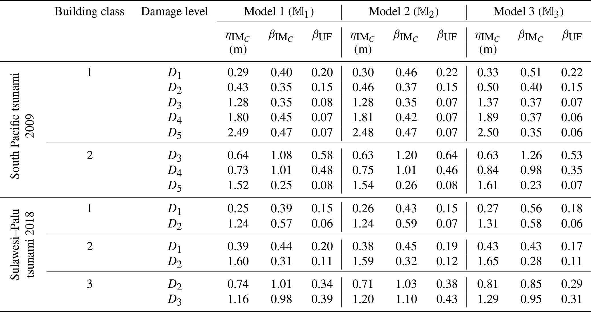
The empirical fragilities derived through the hierarchical fragility procedure are not necessarily attributed to a lognormal distribution. Hence, we have derived equivalent lognormal statistics (i.e. the median and dispersion) for the resulting fragility curves. The median intensity, ${\mathit{\eta }}_{{\mathrm{IM}}_C}$, for a given damage level is calculated as the IM corresponding to 50 % probability on the fragility curve. The logarithmic standard deviation (dispersion) of the equivalent lognormal fragility curve at the onset of damage threshold, ${\mathit{\beta }}_{{\mathrm{IM}}_C}$, is estimated as half of the logarithmic distance between the IMs corresponding to the probabilities of 16 % (${\text{IM}}_C^{\mathrm{16}}$) and the 84 % (${\text{IM}}_C^{\mathrm{84}}$) on the fragility curve; thus, the dispersion can be estimated as ${\mathit{\beta }}_{{\mathrm{IM}}_C}=\mathrm{0.50}\times \ln \left({\text{IM}}_C^{\mathrm{84}}/{\text{IM}}_C^{\mathrm{16}}\right)$. The overall effect of epistemic uncertainties (due to the uncertainty in the fragility model parameters and reflecting the effect of limited sample size) on the median of the empirical fragility curve is considered through (logarithmic) intensity-based standard deviation denoted as β_UF (see Jalayer et al., 2020). β_UF can be estimated as half of the (natural) logarithmic distance (along the IM axis) between the median intensities (i.e. 50 % probability) of the RF's derived with 16 % (denoted as IM⁸⁴) and 84 % (IM¹⁶) confidence levels, respectively; i.e. ${\mathit{\beta }}_{\mathrm{UF}}=\mathrm{0.50}\times \ln \left({\text{IM}}^{\mathrm{84}}/{\text{IM}}^{\mathrm{16}}\right)$. The RF and its confidence band, the sample fragilities θ_k,l (where $l=\mathrm{1}:N_d$), the equivalent lognormal parameters ${\mathit{\eta }}_{{\mathrm{IM}}_C}$ and ${\mathit{\beta }}_{{\mathrm{IM}}_C}$ of the RF, the epistemic uncertainty β_UF, and finally the intensities IM¹⁶ and IM⁸⁴ are shown in Figs. 2d to 6d in the following Sect. 3.

3 Results

3.1 Case study 1: the 2009 South Pacific tsunami

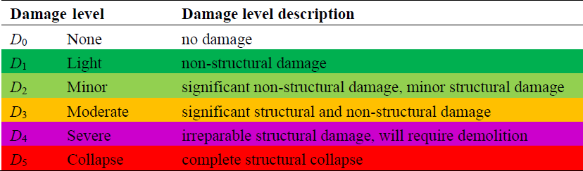
The central South Pacific region-wide tsunami was triggered by an unprecedented earthquake doublet (M_w 8.1 and M_w 8.0) on 29 September 2009, between about 17:48 and 17:50 UTC (Goff and Dominey-Howes, 2011). The tsunami seriously impacted numerous locations in the central South Pacific. Herein, the damage data related to the brick masonry residential (1 storey) and Timber residential buildings associated with the reconnaissance survey sites of American Samoa and the Samoan Islands were utilised. Based on the observed damage regarding different indicators (see Reese et al., 2011 for more details on damage observation), each structure was assigned a damage state between (DS₀ and DS₅). The original data documented in Reese et al. (2011) reporting the tsunami flow depth and the attributed damage state to each surveyed building can be found on the site of the European Tsunami Risk Service (https://eurotsunamirisk.org/datasets/, last access: 30 November 2022). The five damage levels (N_DS=5) and a description of the indicators leading to the classification of the damage states are given in Table 1 based on Reese et al. (2011).

Table 1 The classification of damage thresholds (the damage scale) used for the 2009 South Pacific tsunami (from Reese et al., 2011).

3.2 Case study 2: the 2018 Sulawesi–Palu tsunami

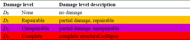
On Friday 28 September 2018, at 18:02 local time, a shallow strike-slip earthquake of moment magnitude M_w 7.5 occurred near Palu City, Central Sulawesi, Indonesia followed by submarine landslides, a tsunami, and massive liquefaction caused substantial damage (Muhari et al., 2018; Rafliana et al., 2022). In Sulawesi, more than 3300 fatalities and missing people, 4400 serious injuries and 170 000 people were displaced by earthquake, tsunami, landslides, liquefaction or building collapse, or combinations of these hazards (Paulik et al., 2019; Mas et al., 2020). Herein, the damage data related to the non-engineered unreinforced clay brick masonry (1 and 2 storey) and non-engineered light timber buildings located in Palu City were utilised. Based on the observed damage (see Paulik et al., 2018 for details on damage observation), each structure was assigned a damage state between (DS₀ and DS₃). The original data reporting the tsunami flow depth and the attributed damage state to each surveyed building can be found as the Supplement to Paulik et al. (2018). The three damage levels (N_DS=3) and a description of the indicators leading to the classification of the damage state are given in Table 2.

Table 2 The classification of damage thresholds (the damage scale) used for the 2018 Sulawesi–Palu tsunami (from Paulik et al., 2019).

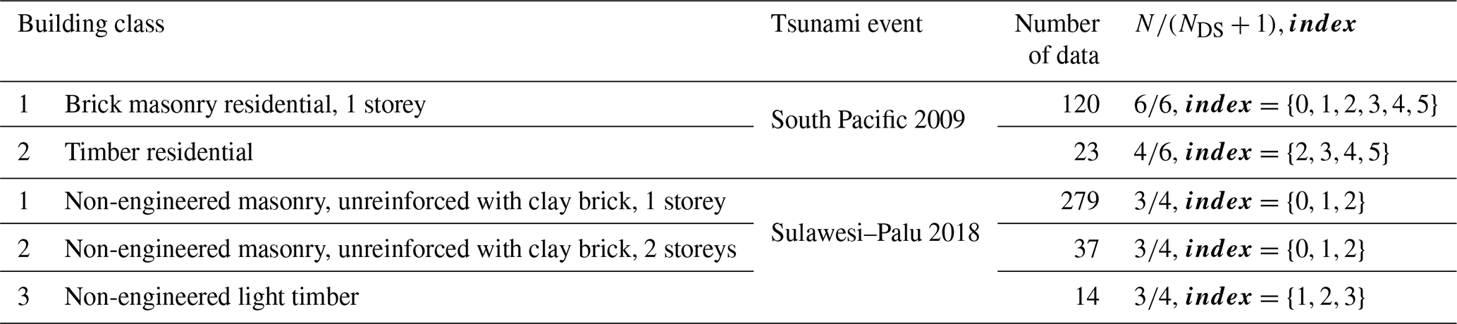
3.3 The building classes

Table 3 illustrates the building classes, for which fragility curves are obtained based on the proposed procedure and based on the databases related to the two tsunami events described above. The taxonomy used for describing the building class matches the original description used in the raw databases. The number of data points available for different building classes showcases both classes with large number of data available, e.g. brick masonry 1 storey (South Pacific) and non-engineered brick masonry 1 storey (Sulawesi), and classes with few data points available, e.g. timber residential (South Pacific) and non-engineered masonry 2 storeys and timber (Sulawesi). The fifth column in the table shows the proportion of the number of damage levels for which observed data are available N (see Sect. 2.1) to the total number of damage levels in the corresponding damage scales, namely $N_{\mathrm{DS}}+\mathrm{1}=\mathrm{6}$ for South Pacific and $N_{\mathrm{DS}}+\mathrm{1}=\mathrm{4}$ for Sulawesi tsunami events (to include level 0). If the ratio is equal to unity, it indicates that data are available for all the damage levels from 0 to N_DS. Note that the number of fragility curves derived is going to be equal to N−1, that is, equal to the number of damage levels for which observed damage data are available minus one.

Table 3 The building classes.

3.4 The different model classes

For each building class considered, we have considered the set of candidate models consisting of the fragility models resulting from the three alternative link functions used in the generalised linear regression in Eq. (5). That is, 𝕄₁ refers to hierarchical fragility modelling based on “logit”, 𝕄₂ refers to hierarchical fragility modelling based on “probit”, and 𝕄₃ refers to hierarchical fragility modelling based on “cloglog”. For each model, both the MLE method using the MATLAB generalised regression toolbox and the BMCS using the procedure described in the previous section are implemented.

3.5 Fragility modelling using MLE

The first step towards fragility assessment by employing the MLE method (see Sect. 2.3) is to define the vector of model parameters $\mathit{\theta }=\left\{{\mathit{\alpha }}_{\mathrm{0},j},{\mathit{\alpha }}_{\mathrm{1},j}\right\}$, where $j=\mathit{i}\mathit{n}\mathit{d}\mathit{e}\mathit{x}(\mathrm{1}:(N-\mathrm{1}\left)\right)$ and where vector index is defined in Sect. 2.1 as the vector of damage level indices (in ascending order) for which observed damage data are available and N is the length of index. To accomplish this, the model parameters $\left\{{\mathit{\alpha }}_{\mathrm{0},j},{\mathit{\alpha }}_{\mathrm{1},j}\right\}$ are obtained by fitting the link functions in Eq. (5) to conditional fragility $P\left(D\ge D_{j+\mathrm{1}}\left|D\ge D_j,\text{IM}\right.\right)$ according to Eq. (6). Herein, we have used MATLAB as a statistical software package (developed by MathWorks) to estimate the maximum likelihood of model parameters $\left\{{\mathit{\alpha }}_{\mathrm{0},j},{\mathit{\alpha }}_{\mathrm{1},j}\right\}$ using the following MATLAB command: glmfit$\left(\log \right({\mathit{x}}_j),{\mathit{y}}_j,\text{`binomial'},\text{`link'},\text{model'})$. The `model' will be either `logit', `probit', or `comploglog'. For each damage level D_j+1, $\mathit{i}\mathit{n}\mathit{d}\mathit{e}\mathit{x}\left(\mathrm{1}\right)\le j<\mathit{i}\mathit{n}\mathit{d}\mathit{e}\mathit{x}\left(N\right)$, the vector x_j is the IM's for which the condition D≥D_j is satisfied; y_j is the column vector containing one-to-one probability assignment to the IM data in x_j, with zero (=0.0) assigned to those data corresponding to DS_j ($D_j\le D<D_{j+\mathrm{1}}$) and one (=1.0) to those related to higher damage states (with $D\ge D_{j+\mathrm{1}}$).

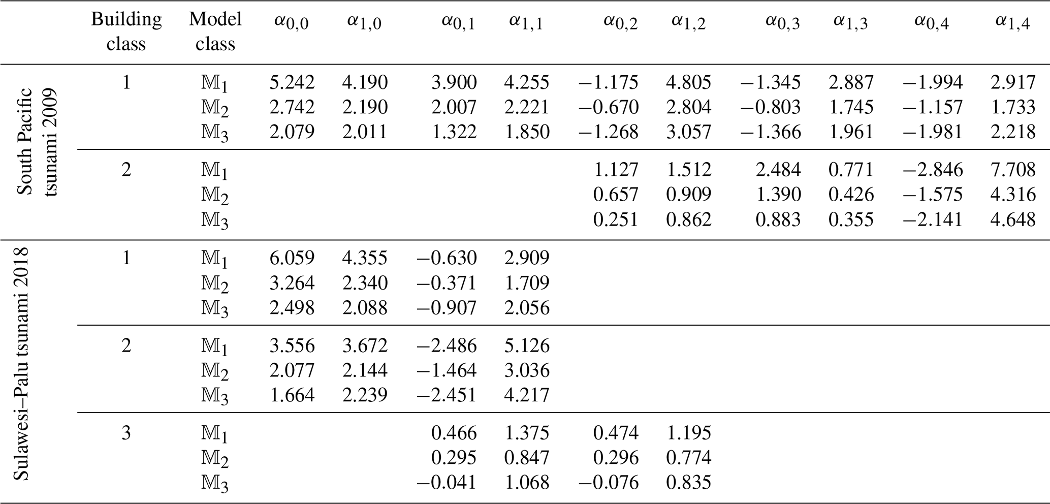
The vectors defining the MLE of the model parameters, θ_MLE, are presented in Table 4 for each of the building classes listed in Table 3 and for each of the three models 𝕄₁, 𝕄₂, and 𝕄₃ defined in Sect. 3.4. Given the model parameter θ_MLE, the damage state probability P(DS_j|IM) can be estimated based on the recursive Eqs. (7) and (8). Then, the fragility for the ultimate damage level is calculated first based on Eq. (8). For the lower damage thresholds, the empirical fragility is derived based on Eq. (9). The resulting hierarchical fragility curves by employing the direct fragility assessment given θ_MLE, i.e. $P(\left.D\ge D_j\right|\text{IM},{\mathit{\theta }}_{\mathrm{MLE}})$ for $j=\mathit{i}\mathit{n}\mathit{d}\mathit{e}\mathit{x}\left(\mathrm{2}:N\right)$, are shown later in the next section by comparison with those obtained from the BMCS method.

Table 4 The model parameters θ_MLE.

3.6 Fragility modelling using BMCS

In the first step, the model parameters are estimated for each model class separately. For each model class 𝕄_k, the model parameters θ_k are estimated through the adaptive MCMC method described in detail in Appendix E, which yields the posterior distribution in Eq. (14). With reference to Eq. (14), the prior joint PDF p(θ_k|𝕄_k) is a multivariate normal PDF with zero correlation between the pairs of model parameters (see Appendix D). The vector of the mean values, μ_θ is set to be the MLE tabulated in Table 4 (=θ_MLE related to 𝕄_k). We have attributed a high value for the coefficient of variation (more than 3.20 herein) for each of the model parameters. Appendix F illustrates the histograms representing the drawn samples from the joint posterior PDF p(θ_k|D,𝕄_k) for a selected building class.

The RF curves derived from the hierarchical fragility curves (see Sect. 2.5) and the corresponding plus/minus 1 standard deviation (±1σ) intervals from Eqs. (16) and (17) are also plotted in Figs. 2a to 6a corresponding to Classes 1–2 South Pacific tsunami and Classes 1–3 Sulawesi–Palu for one of the model classes 𝕄_k $(k\in \left\{\mathrm{1},\mathrm{2},\mathrm{3}\right\})$ and for the damage thresholds D_j, $j=\mathit{i}\mathit{n}\mathit{d}\mathit{e}\mathit{x}\left(\mathrm{2}:N\right)$. The colours of the hierarchical robust fragility curves, labelled as D_j-BMCS, match closely with those shown in Tables 1 and 2. The corresponding ±1σ confidence interval curve, which reflects the uncertainty in the model parameters, is shown as a light grey area with different colour intensities. Figures 2b to 6b compare the hierarchical robust fragility and its confidence interval with the result of hierarchical fragility assessment based on maximum likelihood estimation (see previous Sect. 3.5) labelled as D_j-MLE. The fragility curves are shown with similar colours (and darker intensity) and with the same line type (and half of the thickness) of the corresponding robust fragility curves. The first observation is that the results of MLE-based fragilities and the BMCS-based fragilities are quite close in all damage thresholds (as expected, see Jalayer and Erahimian, 2020). Moreover, the BMCS provides also the confidence bands for the fragility curves, which cannot be directly provided by the MLE method. To showcase an individual fragility curve, Figs. 2c to 6c illustrate the empirical fragility curves associated with the lth realisation of the vector of model parameters θ_k,l for model class 𝕄_k (where l is defined on each figure separately), i.e. $P(\left.D\ge D_j\right|\text{IM},{\mathit{\theta }}_{k,l})$ (see Sect. 2.5). Figures 2d to 6d illustrate the robust fragility curve associated with the ultimate damage threshold D_index(N), together with all the sample fragilities. The intensity values for which the damage level is not exceeded are shown with blue circles having the probability equal to zero. Other IMs that lead to the exceedance of the damage level are shown with red circles with a probability equal to one. Figures 2d to 6d also illustrate all the fragility parameters described in Sect. 2.5 including the equivalent lognormal parameters ${\mathit{\eta }}_{{\mathrm{IM}}_C}$ and ${\mathit{\beta }}_{{\mathrm{IM}}_C}$; the epistemic uncertainty in the empirical fragility assessment β_UF; and also the intensities ${\text{IM}}_C^{\mathrm{16}}$, ${\text{IM}}_C^{\mathrm{84}}$, IM⁸⁴, and IM¹⁶ (the latter two are IMs at the median, i.e. 50 % probability, from the RF ±1 standard deviation, respectively. For all five building classes considered (see Table 3), ${\mathit{\eta }}_{{\mathrm{IM}}_C}$, ${\mathit{\beta }}_{{\mathrm{IM}}_C}$, and β_UF are tabulated in Table 5 for all damage thresholds associated to model classes 𝕄₁ to 𝕄₃.

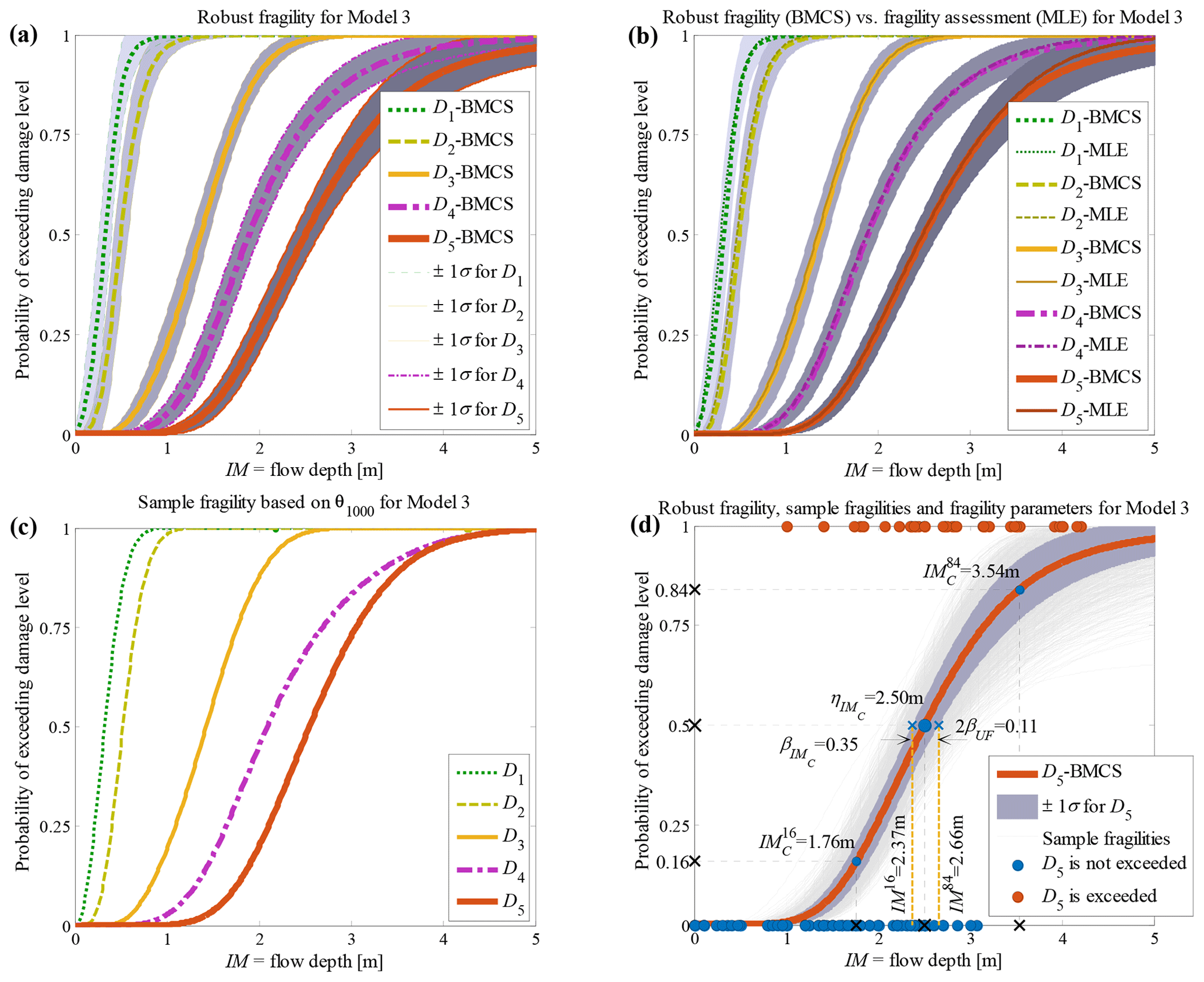
Figure 2 Building class 1 (brick masonry residential, 1 storey) of the South Pacific 2009 tsunami considering fragility model class 𝕄₃ (a) hierarchical robust fragility curves and their ±1 standard deviation confidence intervals; (b) comparison between hierarchical robust fragility curves and their confidence band (based on BMCS method) and fragility assessment based on MLE method; (c) the fragility curves $P\left(\left.D\ge D_j\right|\text{IM},{\mathit{\theta }}_{\mathrm{3},\mathrm{1000}}\right)$, where $\mathrm{1}\le j\le \mathrm{5}$ associated with the 1000th realisation of the model parameters, θ_3,1000 (k=3 associated to model 𝕄₃, l=1000); and (d) RF associated with the damage threshold D₅, together with all the sample fragilities and the equivalent lognormal fragility parameters.

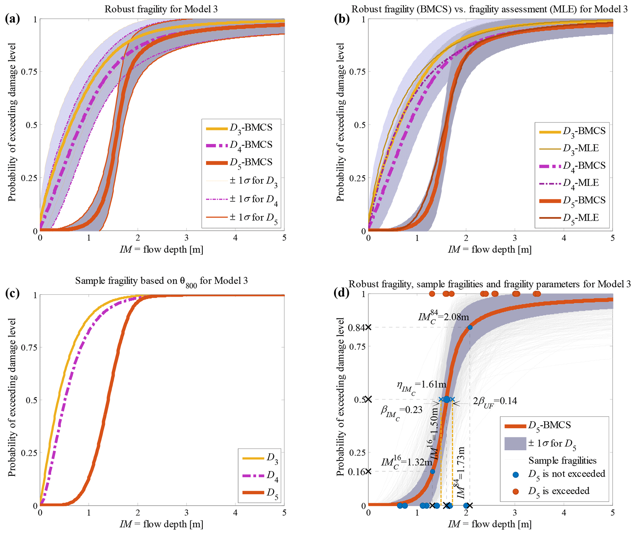
Figure 3 Building class 2 (timber residential) of the South Pacific 2009 tsunami considering fragility model class 𝕄₃ (a) hierarchical robust fragility curves and their ±1 standard deviation confidence intervals; (b) comparison between hierarchical robust fragility curves and their confidence band (based on BMCS method) and fragility assessment (based on MLE method); (c) the fragility curves $P(\left.D\ge D_j\right|\text{IM},{\mathit{\theta }}_{\mathrm{3},\mathrm{800}})$ where $\mathrm{3}\le j\le \mathrm{5}$ associated with the 800th realisation of the model parameters, θ_3,800 (k=3 associated to model 𝕄₃, l=800); and (d) robust fragility associated with the damage threshold D₅, together with all the sample fragilities and the equivalent lognormal fragility parameters.

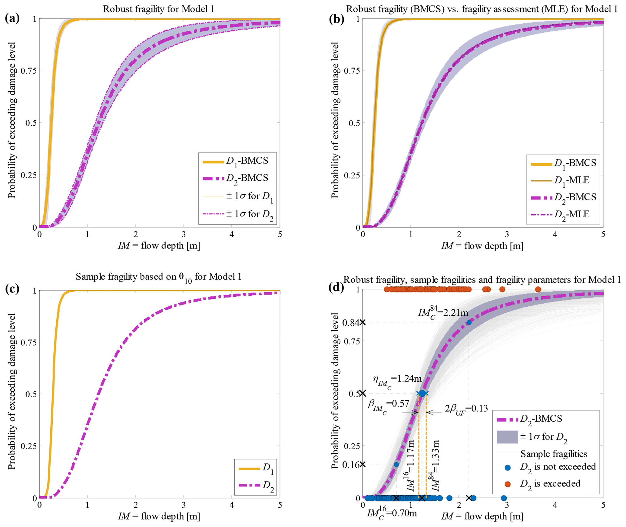
Figure 4 Building class 1 (non-engineered masonry, unreinforced with clay brick, 1 storey) of the Sulawesi–Palu 2018 tsunami considering fragility model class 𝕄₁ (a) robust fragility curves (RF) and their ±1 standard deviation confidence intervals; (b) comparison between hierarchical robust fragility and its confidence band (based on BMCS method) and fragility assessment based on MLE method; (c) the fragility curves $P(\left.D\ge D_j\right|\text{IM},{\mathit{\theta }}_{\mathrm{1},\mathrm{10}})$, where $\mathrm{1}\le j\le \mathrm{2}$ associated with the 10th realisation of the model parameters, θ_1,10 (k=1 associated to model 𝕄₁, l=10); and (d) robust fragility curve associated with the damage threshold D₂, together with all the sample fragilities and the equivalent lognormal fragility parameters.

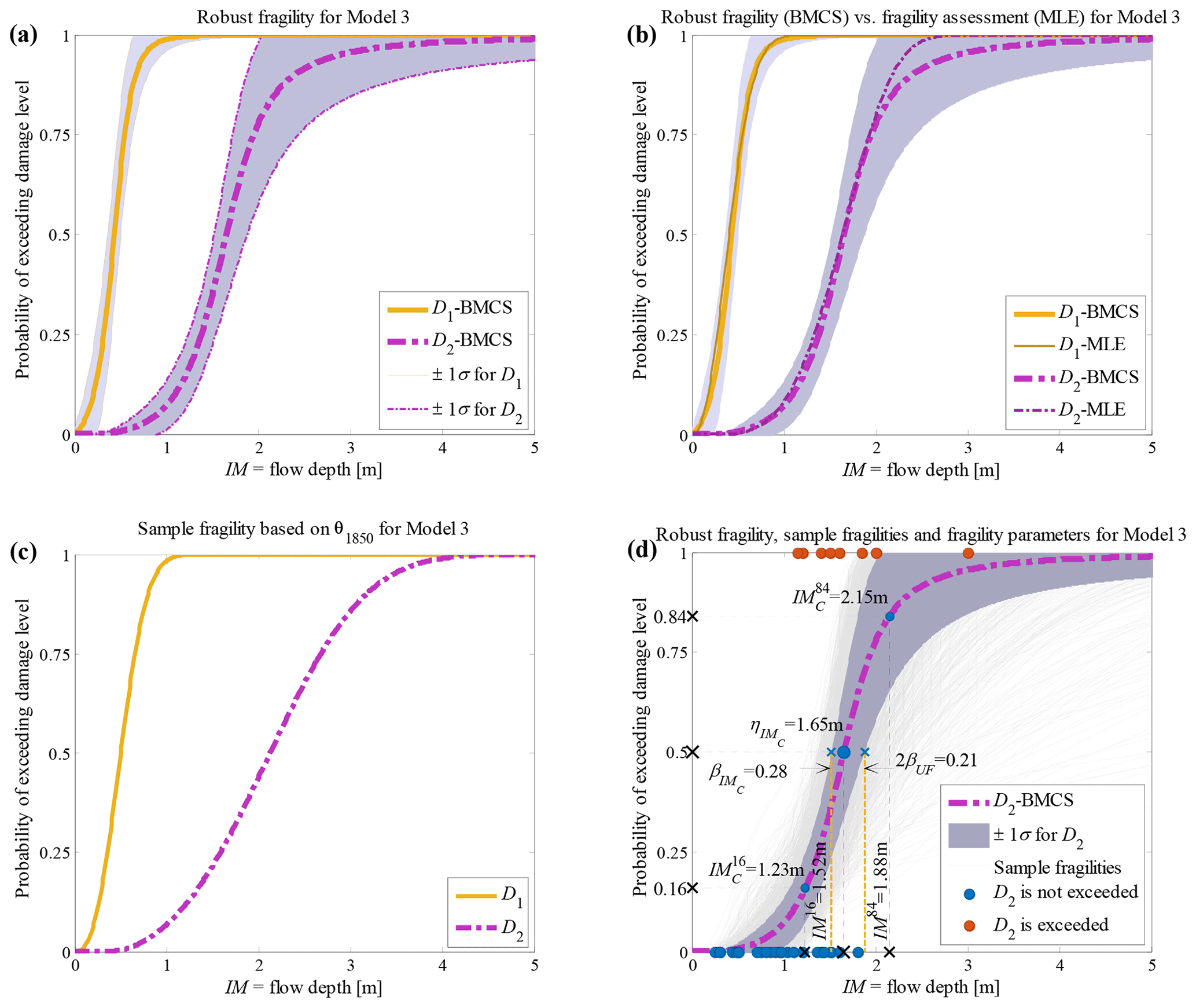
Figure 5 Building class 2 (non-engineered masonry, unreinforced with clay brick, 2 storey) of the Sulawesi–Palu 2018 tsunami considering fragility model class 𝕄₃ (a) hierarchical robust fragility curves and their ±1 standard deviation confidence intervals; (b) comparison between robust fragility and its confidence band (based on BMCS method) and fragility assessment based on MLE method; (c) the fragility curves $P(\left.D\ge D_j\right|\text{IM},{\mathit{\theta }}_{\mathrm{3},\mathrm{1850}})$, where $\mathrm{1}\le j\le \mathrm{2}$ associated with the 1850th realisation of the model parameters, θ_3,1850 (k=3 associated to model 𝕄₃, l=1850); and (d) robust fragility curve associated with the damage threshold D₂, together with all the sample fragilities and the equivalent lognormal fragility parameters.

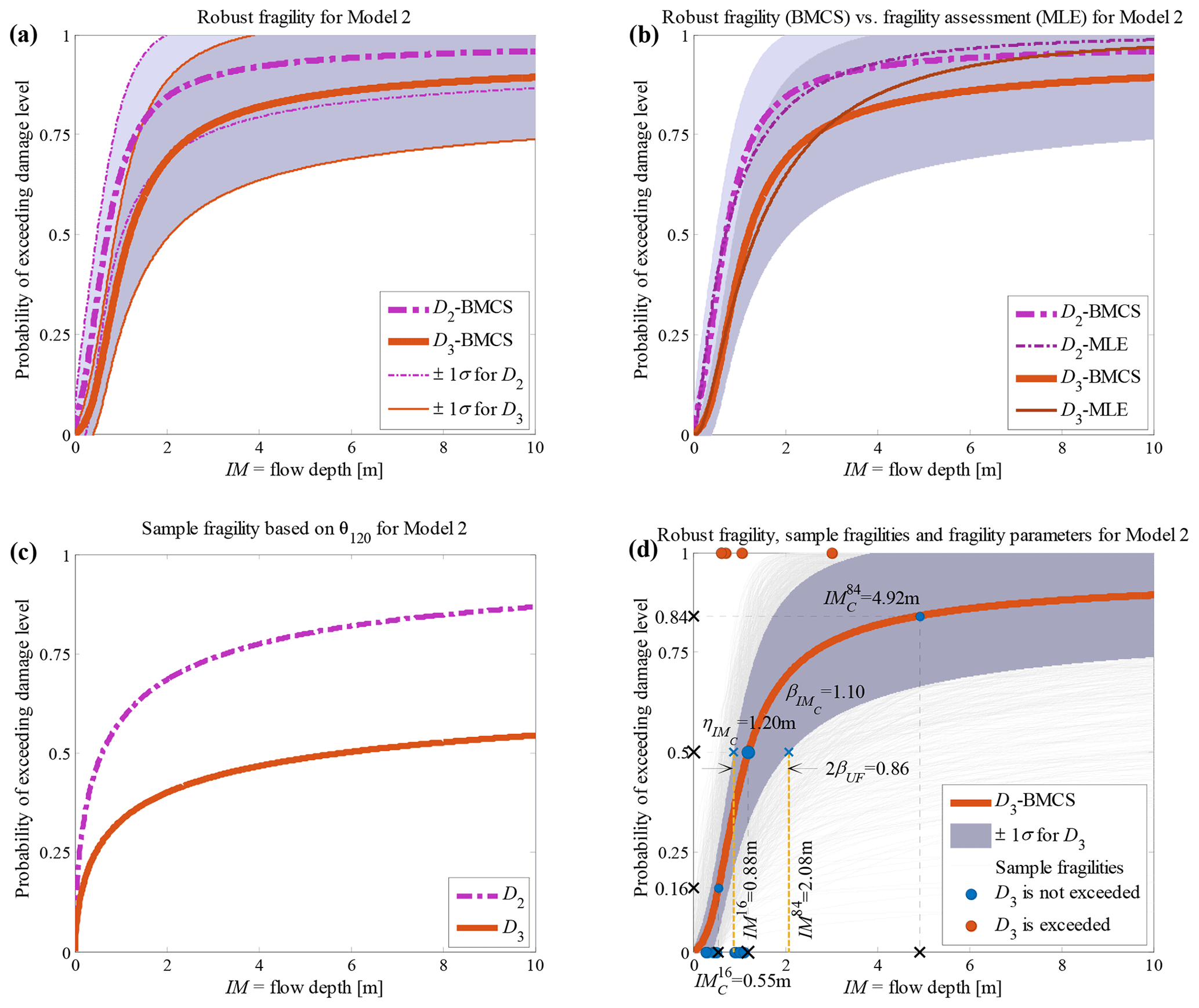
Figure 6 Building class 3 (non-engineered light timber) of the Sulawesi–Palu 2018 tsunami considering fragility model class 𝕄₂ (a) hierarchical robust fragility curves and their ±1 standard deviation confidence intervals; (b) comparison between robust fragility and its confidence band (based on BMCS method) and fragility assessment based on MLE method; (c) the fragility curves $P(\left.D\ge D_j\right|\text{IM},{\mathit{\theta }}_{\mathrm{2},\mathrm{120}})$, where $\mathrm{2}\le j\le \mathrm{3}$ associated with the 120th realisation of the model parameters, θ_2,120 (k=2 associated to model 𝕄₂, l=120); and (d) robust fragility curve associated with the damage threshold D₃, together with all the sample fragilities and the equivalent lognormal fragility parameters.

Table 5 The equivalent lognormal parameters and the epistemic uncertainty in the RF assessment for all the building classes, damage thresholds, and model classes 𝕄₁ to 𝕄₃.

3.7 Model selection

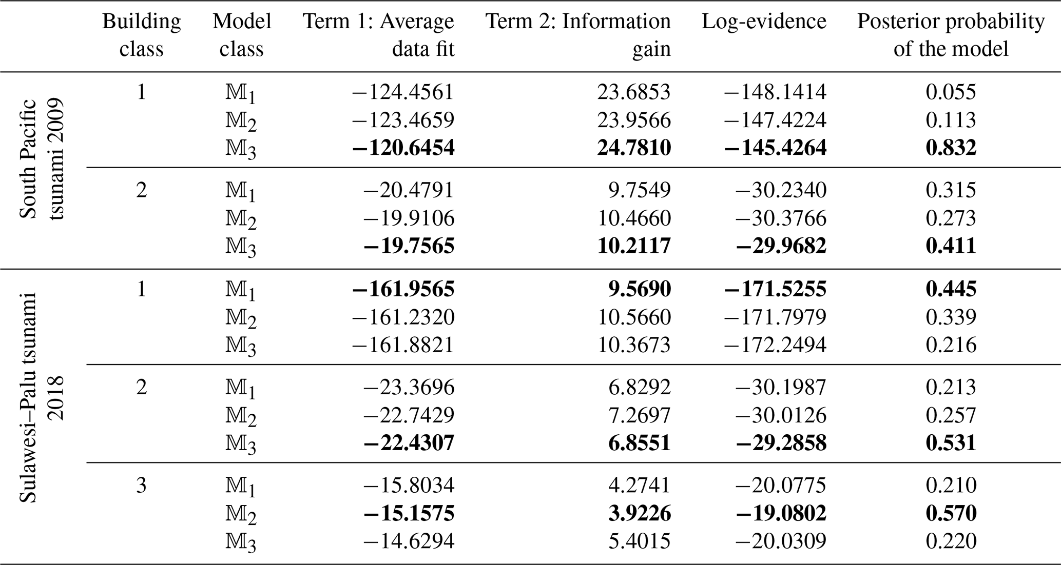
With reference to Eq. (12), the log-evidence ln [p(D|𝕄_k)] can be estimated by subtracting Term 2 from Term 1. Term 1 denotes the posterior mean of the log likelihood, and Term 2 is the relative entropy between the prior and the posterior. Within the BMCS method, these two terms are readily computable.

Given the samples generated from the joint posterior PDFs θ_k, Term 1 (the average data fit) can be seen as the expected value of the log likelihood over the vector of fragility parameters θ_k given the model 𝕄_k, i.e. ${\mathrm{E}}_{\left.{\mathit{\theta }}_k\right|\mathit{D},{\mathbb{M}}_k}\left(\ln \left[p\left(\mathit{D}\mathrm{|}{\mathbb{M}}_k\right)\right]\right)$. Term 2 (the relative entropy) is calculated as the expected value of information gain or entropy between the two PDFs posterior and prior over the vector θ given the model 𝕄_k, i.e. ${\mathrm{E}}_{\left.{\mathit{\theta }}_k\right|\mathbf{D},{\mathbb{M}}_k}\left(\ln \left[p({\mathit{\theta }}_k\mathrm{|}\mathit{D},{\mathbb{M}}_k)/p\left({\mathit{\theta }}_k\mathrm{|}{\mathbb{M}}_k\right)\right]\right)$. It is noted that based on Jensen's inequality, the mean information gain (relative entropy) of the posterior compared to the prior is always non-negative (see e.g. Jalayer et al., 2012; Ebrahimian and Jalayer, 2021). Hence, Term 2 should always be positive. Herein, p(θ_k|D,𝕄_k) is constructed by an adaptive kernel density function (see Eq. E5, Appendix E) as the weighted sum (average) of Gaussian PDFs centred among the samples θ_k given model 𝕄_k ($k=\mathrm{1}:\mathrm{3}$). The prior p(θ_k|𝕄_k) is a multivariate normal PDF, respectively, with the mean and covariance described previously for each model (see Eq. D1 in Appendix D). Table 6 shows the results for model class selection for all five building classes considered. The last column illustrates the posterior probability (weight) of the model P(𝕄_k|D) according to Eq. (10) assuming that the prior $P\left({\mathbb{M}}_k\right)=\frac{\mathrm{1}}{\mathrm{3}}$ (where $k=\mathrm{1}:\mathrm{3}$). The best model for each building class is shown in bold.

For instance, for Class 1 (masonry residential) for the South Pacific tsunami, model class 𝕄₃ (using a complementary log–log “cloglog” transformation of π_ij to the linear logarithmic space, see Eq. 5) is preferred, since it has an overall larger difference between data fit and mean information gain, which leads to a higher log-evidence. The posterior weights (last column of Table 6, see also Eq. 10) of 6 %, 11 % and 83 % are stabilised through different runs of the BMCS method. It should be noted that in Figs. 2 to 6 we reported directly the fragility results for the “best” fragility model class (i.e. the one that maximises log evidence) identified based on the procedure described here.

Table 6 Bayesian model class selection results for empirical fragility models. The best model for each building class is shown in bold.

3.8 The “basic” (MLE-Basic) method: fitting data to one damage state at a time

In the basic method (see Sect. 2.2), the fragility P(D≥D_j|IM) is obtained by using a generalised linear regression model according to Eq. (5) with logit, probit or cloglog link function fitted to the damage data (𝕄_k where $k=\mathrm{1}:\mathrm{3}$). With reference to the MLE method described previously, the vector x_j herein is the IM associated with all damage data (and not partial, as in the hierarchical fragility method described in Sect. 3.3), and y_j is the column vector of one-to-one probability assignment to the IM data in x_j, with zero (=0) assigned to those data with an observed damage threshold D<D_j and one (=1) to those with D≥D_j. Thus, for the empirical fragility associated with the damage threshold D_j, and based on the model 𝕄_k, there are two model parameters to be defined, namely ${\mathit{\theta }}_{\mathrm{MLE}\text{-}Basic}={\left\{{\mathit{\alpha }}_{\mathrm{0}},{\mathit{\alpha }}_{\mathrm{1}}\right\}}_k$. As noted previously, there might be conditions (depending on the quantity of the observed damage data) where a part of the fragility of damage threshold D_j lies below the fragility of the higher damage level D_j+1, indicating that $P\left(\left.{\text{DS}}_j\right|\text{IM}\right)<\mathrm{0}.$ This is due to the fact that in the traditional method there is no explicit requirement to satisfy P(DS_j|IM)>0 as compared to the proposed method. The MLE of model parameters {α₀,α₁} for the damage levels D_j, $j=\mathit{i}\mathit{n}\mathit{d}\mathit{e}\mathit{x}\left(\mathrm{2}:N\right)$ associated with the building classes in Table 3 are presented in Table 7.

Table 7 The Model parameters θ_MLE-Basic.

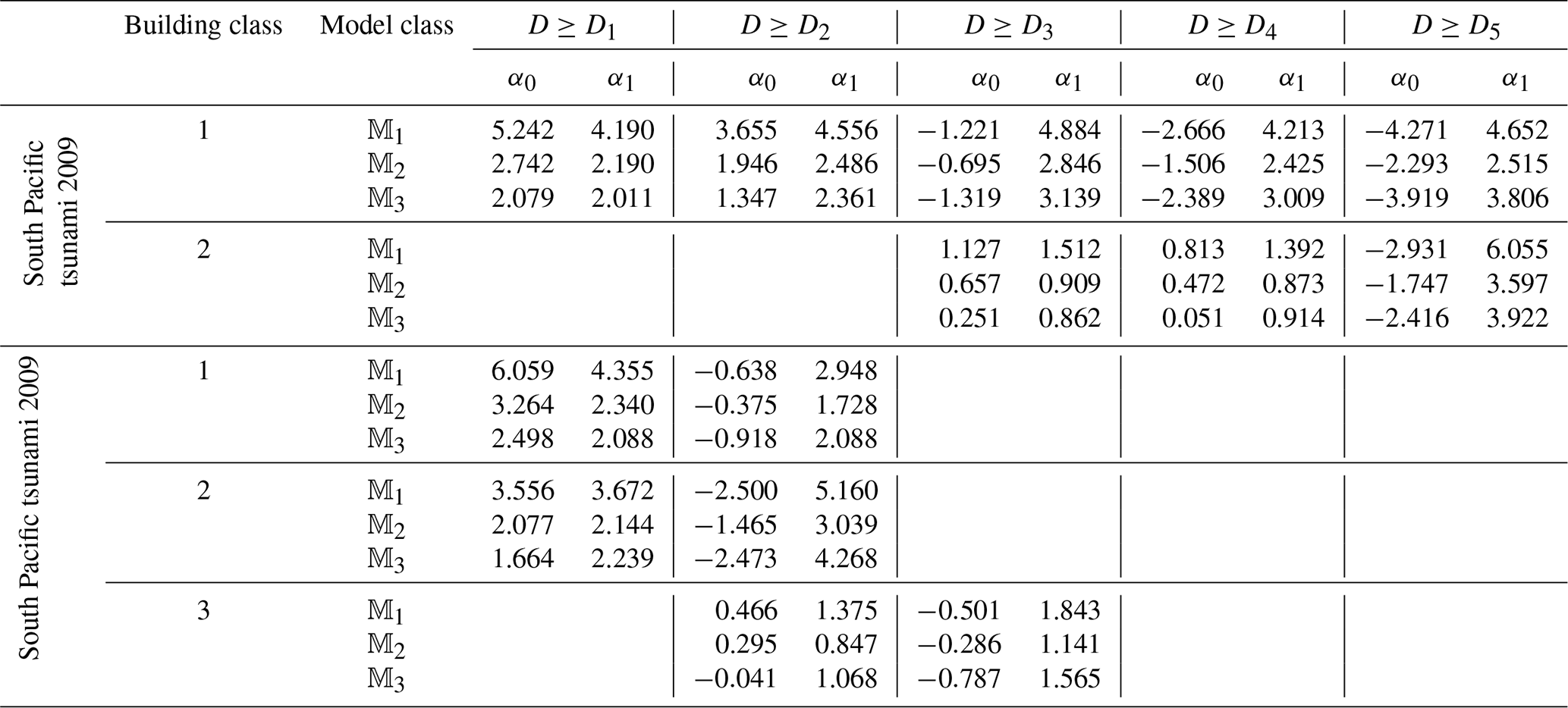
Figure 7 compares the fragility assessment obtained based on MLE-based hierarchical fragility modelling (see also the MLE-based curves in Figs. 2b to 6b) with the result of the fragility assessment by employing the MLE-Basic method for the “best” model class 𝕄_k $(k\in \left\{\mathrm{1},\mathrm{2},\mathrm{3}\right\})$ identified according to the procedure outlined in the previous section. It is noted that the fragility functional form is different between the two methods. MLE-based fragility assessment given 𝕄_k uses Eqs. (7) to (9) to construct a hierarchical fragility curve given that the conditional fragility term ${\mathit{\pi }}_{ij}=P(D\ge D_{j+\mathrm{1}}\left|D\ge D_j,{\text{IM}}_i\right.)$, $j=\mathit{i}\mathit{n}\mathit{d}\mathit{e}\mathit{x}\left(\mathrm{1}:N-\mathrm{1}\right)$ has one of the functional forms in Eq. (5). However, the fragility assessment using the MLE-Basic method employs directly one of the expressions in Eq. (5) (corresponding to 𝕄_k, $k=\mathrm{1}:\mathrm{3}$) to derive the fragility curve ${\mathit{\pi }}_{ij}=P(D\ge D_j\left|{\text{IM}}_i\right.)$ (based on the whole damage data) and $j=\mathit{i}\mathit{n}\mathit{d}\mathit{e}\mathit{x}(\mathrm{2}:N)$. This difference manifests itself in Fig. 7a (for brick masonry residential, Class 1, South Pacific tsunami) as the deviation between the two fragility models for higher damage thresholds D₄ and D₅. The deviations between the fragility curves are particularly noticeable at higher IM values (with exceedance probability >50 %); however, their medians are quite similar. In Fig. 7b for (timber residential buildings, Class 2, South Pacific tsunami) and 7e (light informal timber buildings, Class 3, Sulawesi–Palu tsunami), we can observe that fragility curves intersect in the case of the MLE-Basic fragility assessment. However, they do not intersect for hierarchical fragility curves. The intersection points of the consequent damage states D_j+1 with D_j when using the MLE-Basic fragility estimation method are shown with colour stars on each figure.

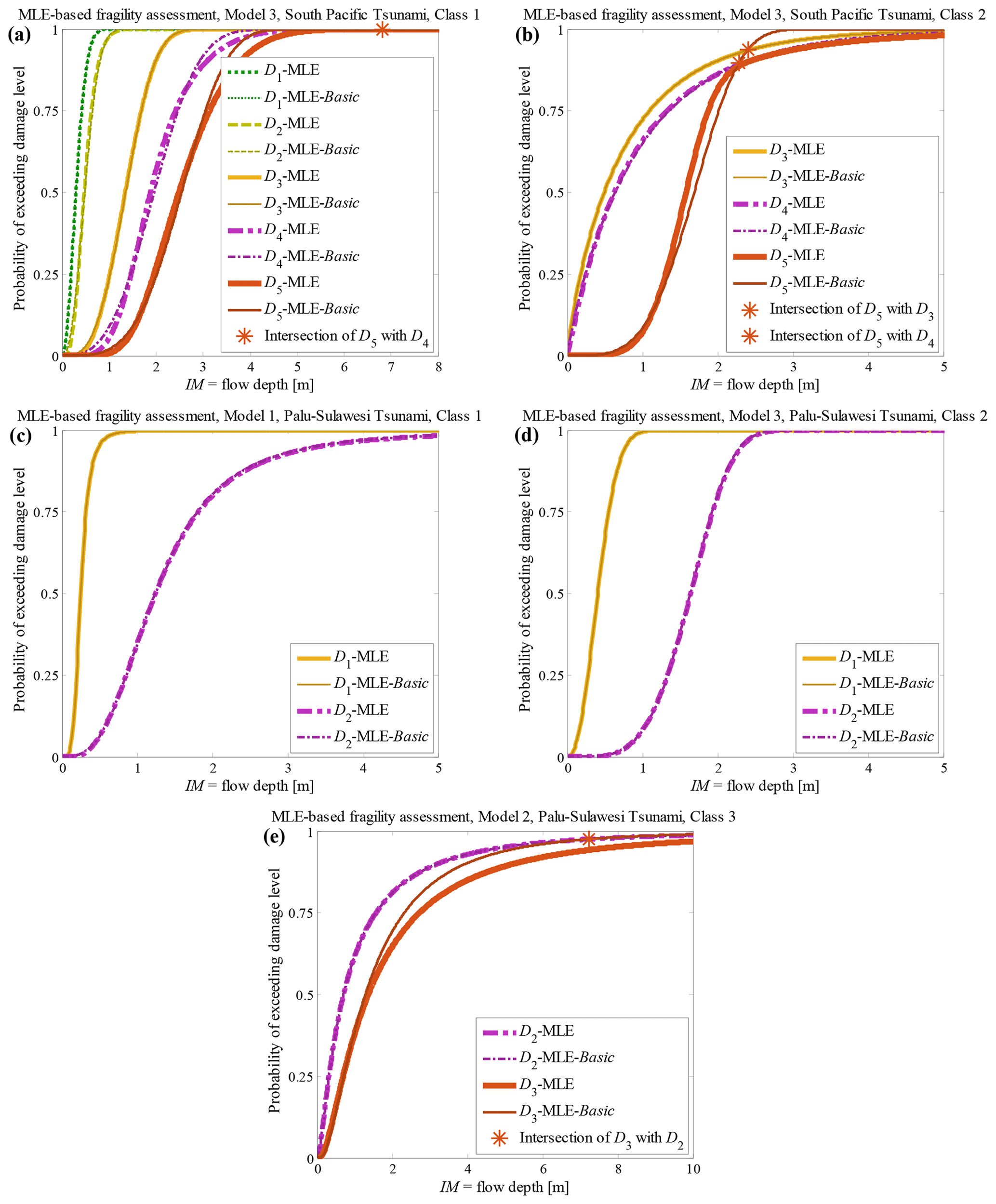
Figure 7 Comparison between the fragility assessment by MLE-based hierarchical fragility modelling and MLE-Basic fragility assessment given (a) South Pacific 2009 tsunami, Class 1, 𝕄₃; (b) South Pacific 2009 tsunami, Class 2, 𝕄₃; (c) Sulawesi–Palu 2018 tsunami, Class 1, 𝕄₁; (d) Sulawesi–Palu 2018 tsunami Class 2, 𝕄₃; and (e) Sulawesi–Palu 2018 tsunami Class 3, 𝕄₂.

Table 8 reports the fragility assessment parameters of the MLE and MLE-Basic methods for the damage thresholds D_index(2) to D_index(N) with the equivalent lognormal parameters ${\mathit{\eta }}_{{\mathrm{IM}}_C}$ and ${\mathit{\beta }}_{{\mathrm{IM}}_C}$ (explained in Sect. 2.5) for 𝕄₁ to 𝕄₃ for all five classes considered. The medians are almost identical among the four models while there are higher dispersion estimates for the MLE method derived by hierarchical fragility modelling.

Table 8 Comparison between fragility assessment based on MLE method (by hierarchical fragility modelling) and the MLE-Basic method for damage thresholds D_index(2) to D_index(N).

4 Discussion

The results outlined in this section show a fragility assessment for two different data sets corresponding to observed damaged in the aftermath of South Pacific and Sulawesi–Palu tsunami events. We have demonstrated the versatility of the proposed workflow and tool for hierarchical fragility assessment both for cases in which a large number of data points are available (e.g. Class 1, brick masonry residential, South Pacific tsunami; Class 1, one-storey non-engineered masonry, Sulawesi–Palu tsunami) and cases where very few data points are available (e.g. Class 2, timber residential, South Pacific tsunami; Class 3, non-engineered light timber, Sulawesi–Palu tsunami). Moreover, we demonstrated how the proposed workflow avoids crossing fragility curves (e.g. Class 2, timber residential, South Pacific tsunami; Class 3, non-engineered light timber, Sulawesi–Palu tsunami). The results illustrated for the five building classes demonstrate that the proposed workflow for hierarchical fragility assessment can be applied in cases in which data points are not available for all the damage levels within the damage scale.

5 Conclusion

An integrated procedure based on Bayesian model class selection (BMCS) for empirical hierarchical fragility modelling for a class of buildings or infrastructure is presented. This procedure is applicable to fragility modelling for any type of hazard as long as the damage scale consists of mutually exclusive and collectively exhaustive (MECE) damage states, and the observed damage data points are independent. This simulation-based procedure can (1) perform hierarchical fragility modelling for MECE damage states, (2) estimate the confidence interval for the resulting fragility curves, and (3) select the simplest model that fits the data best (i.e. maximises log evidence) amongst a suite of candidate fragility models (herein, alternative link functions for generalised linear regression are considered). The proposed procedure is demonstrated for empirical fragility assessment based on observed damage data to masonry residential (1 storey) and timber residential buildings due to the 2009 South Pacific tsunami in American Samoa and the Samoan Islands and non-engineered masonry buildings (1 and 2 storeys) and non-engineered light timber buildings due to the 2018 Sulawesi–Palu tsunami. It is observed that

• For each model class, the same set of simulation realisations is used to estimate the fragility parameters, the confidence band and the log evidence. The latter, which consists of two terms depicting the goodness of fit and the information gain between posterior distribution resulting from the observed data and the prior distribution, is used to compare the candidate fragility models to identify the model that maximises the evidence.

• Hierarchical fragility assessment can be done also based the maximum likelihood estimation (MLE) and the available statistical toolboxes (e.g. MATLAB's generalised linear model). For each damage level, the reference domain should be the subset of data that exceeds the consecutive lower damage level, instead of taking the entire set of data points as reference domain. Note that the basic fragility estimation (“MLE-Basic”, non-hierarchical fragility model) fits the damage data for each damage level at a time. In other words, the reference domain is set to all damage data.

• The procedure is also applicable to cases in which observed data are available only for a subset of the damage levels within the damage scale. The number of fragility curves is going to be equal to the total number of damage levels for which data are available minus one. This means, in order to have at least one fragility curve, one needs to have data available for at least two damage levels.

• Although the resulting fragility curves are not lognormal (strictly speaking), equivalent statistics work quite well in showing the fragility curves (median and logarithmic dispersion) and the corresponding epistemic uncertainty (logarithmic dispersion).

• The proposed BMCS method and the one based on MLE lead to essentially the same set of parameter estimates for hierarchical fragility estimation. However, the latter does not readily lead to the confidence band and log evidence.

• Using the basic method for fragility estimation (MLE-Basic) leads to results that are slightly different from the hierarchical fragility curves. The difference grows for higher damage levels. It is important to note that following the basic method MLE-Basic led to ill-conditioned results (i.e. fragility curves crossing) in some of the cases (Class 2 for the South Pacific tsunami and Class 3 for the Sulawesi–Palu tsunami, both Timber constructions) studied in this work.

The major improvement offered by this method is in providing a tool that can fit fragility curves to a set of hierarchical levels of damage or loss in an ensemble manner. This method, which starts from prescribed fragility models and explicitly ensures the hierarchical relation between the damage levels, is very robust in cases where few data points are available and/or where data are missing for some of the damage levels. This tool provides confidence bands for the fragility curves and performs model selection among a set of viable link functions for generalised regression. It is important to note that the proposed method is in general applicable to hierarchical vulnerability modelling for human or economic loss levels and to different types of hazards if (1) the defined levels are mutually exclusive and collectively exhaustive, and (2) a suitable intensity measure (IM) can be identified.

Appendix A: The derivation of Eq. (2)

The probability of being in damage state DS_j for a given intensity measure IM can be estimated as follows:

$$\begin{array}{}\text{(A1)}& \begin{array}{rl}& P\left({\text{DS}}_j|\text{IM}\right)\\ & =P\left[(D\ge D_j)\cdot (D<D_{j+\mathrm{1}})|\text{IM}\right]\\ & =\mathrm{1}-P\left[\stackrel{\mathrm{‾}}{(D\ge D_j)\cdot (D<D_{j+\mathrm{1}})}|\text{IM}\right]\\ & =\mathrm{1}-P\left[\stackrel{\mathrm{‾}}{(D\ge D_j)}+\stackrel{\mathrm{‾}}{(D<D_{j+\mathrm{1}})}|\text{IM}\right]\\ & =\mathrm{1}-\underset{\mathrm{ME}\triangleq P(D<D_j|\text{IM})+P(D\ge D_{j+\mathrm{1}}\left|\text{IM}\right)}{\underbrace{P\left[(D<D_j)+(D\ge D_{j+\mathrm{1}})|\text{IM}\right]}}\\ & =\mathrm{1}-P(D<D_j|\text{IM})-P(D\ge D_{j+\mathrm{1}}\left|\text{IM}\right)\\ & =P(D\ge D_j|\text{IM})-P(D\ge D_{j+\mathrm{1}}\left|\text{IM}\right)\end{array},\end{array}$$

where the upper-bar sign stands for the logical negation and is read as “NOT”, and (+) defines the logical sum and is read as “OR”. The above derivation is based on the rule of sum in probability and considers the fact that the two statements D<D_j and $D\ge D_{j+\mathrm{1}}$ are mutually exclusive (ME); thus, the probability of their logical sum is the sum of their probabilities.

Appendix B: The derivation of Eq. (7)

The probability of being in damage state DS_j (where j≥1) given the intensity measure evaluated at the location of building i, denoted as IM_i, based on Eq. (6) can be expanded in a recursive format as follows:

$$\begin{array}{}\text{(B1)}& \begin{array}{rl}& P\left(D{S}_j\right|{\text{IM}}_i)\\ & =\underset{\mathrm{1}-{\mathit{\pi }}_{ij}}{\underbrace{\left[\mathrm{1}-P(D\ge D_{j+\mathrm{1}}|D\ge D_j,{\text{IM}}_i)\right]}}\\ & \cdot \left[\mathrm{1}-P(D<D_j|{\text{IM}}_i)\right]\\ & =\left(\mathrm{1}-{\mathit{\pi }}_{ij}\right)\cdot [\mathrm{1}-P((D<D_j)\cdot \left(D\ge D_{j-\mathrm{1}}\right)+\mathrm{\cdots }\\ & +(D<D_{\mathrm{1}})\cdot (D\ge D_{\mathrm{0}})\left|{\text{IM}}_i\right)]\\ & =(\mathrm{1}-{\mathit{\pi }}_{ij})\cdot \left[\mathrm{1}-\sum _{k=\mathrm{0}}^{j-\mathrm{1}}P\left(\right(D<D_{k+\mathrm{1}})\cdot (D\ge D_k\left)\right|{\text{IM}}_i)\right]\\ & =(\mathrm{1}-{\mathit{\pi }}_{ij})\cdot \left[\mathrm{1}-\sum _{k=\mathrm{0}}^{j-\mathrm{1}}P\left({\text{DS}}_k\right|\text{IM})\right]\end{array},\end{array}$$

where (+) defines the logical sum and is read as “OR”. The above derivation is based on the rule of sum in probability and considers the fact that the recursive statements in the second term expressed generally as $(D<D_{k+\mathrm{1}})\cdot (D\ge D_k)$, where $\mathrm{0}\le k\le j-\mathrm{1}$, are ME; hence, the probability of their logical sum is the sum of their probabilities. It is important to note that in case where j=0, the above equation can be written as

$$\begin{array}{}\text{(B2)}& P\left({\text{DS}}_{\mathrm{0}}\right|{\text{IM}}_i)=\left(\mathrm{1}-{\mathit{\pi }}_{i\mathrm{0}}\right)\triangleq P(D<D_{\mathrm{1}}\left|{\text{IM}}_i\right).\end{array}$$

Appendix C: The derivation of log-evidence in Eq. (13)

From an information-based point of view, the logarithm of the evidence (log-evidence), denoted as ln [p(D|𝕄_k)], can provide a quantitative measure of the amount of information as evidence of model 𝕄_k. Moreover, the posterior PDF p(θ_k|D,𝕄_k) (see Eq. 14) over the domain of the model parameters Ω_θ given the kth model is equal to unity. Thus, ln [p(D|𝕄_k)] can be written as follows:

$$\begin{array}{}\text{(C1)}& \begin{array}{rl}\ln \left[p\left(\mathit{D}|{\mathbb{M}}_k\right)\right]=& \ln \left[p\left(\mathit{D}|{\mathbb{M}}_k\right)\right]\\ & \cdot \underset{=\mathrm{1.0}}{\underbrace{\underset{\mathrm{\Omega }{\mathit{\theta }}_k}{\int }p\left({\mathit{\theta }}_k|\mathit{D},{\mathbb{M}}_k\right)\mathrm{d}{\mathit{\theta }}_k}}\end{array}.\end{array}$$

Since the log-evidence is independent of θ, we can bring it inside the integral and do some simple manipulation (also using the relation in Eq. 11) as follows:

$$\begin{array}{}\text{(C2)}& \begin{array}{rl}& \ln \left[p\left(\mathit{D}|{\mathbb{M}}_k\right)\right]=\underset{\mathrm{\Omega }{\mathit{\theta }}_k}{\int }\ln \left[p\left(\mathit{D}|{\mathbb{M}}_k\right)\right]\cdot p\left({\mathit{\theta }}_k|\mathit{D},{\mathbb{M}}_k\right)\mathrm{d}{\mathit{\theta }}_k\\ & =\underset{{\mathrm{\Omega }}_{\mathit{\theta }}}{\int }\ln \left[{\displaystyle \frac{p\left(\mathit{D}|{\mathit{\theta }}_k,{\mathbb{M}}_k\right)p\left({\mathit{\theta }}_k|{\mathbb{M}}_k\right)}{p\left({\mathit{\theta }}_k|\mathit{D},{\mathbb{M}}_k\right)}}\right]\cdot p\left({\mathit{\theta }}_k|\mathit{D},{\mathbb{M}}_k\right)\mathrm{d}{\mathit{\theta }}_k\\ & =\underset{{\mathrm{\Omega }}_{\mathit{\theta }}}{\int }\ln \left[{\displaystyle \frac{p\left(\mathit{D}|{\mathit{\theta }}_k,{\mathbb{M}}_k\right)}{p\left({\mathit{\theta }}_k|\mathit{D},{\mathbb{M}}_k\right)/p\left({\mathit{\theta }}_k|{\mathbb{M}}_k\right)}}\right]\cdot p\left({\mathit{\theta }}_k|\mathit{D},{\mathbb{M}}_k\right)\mathrm{d}{\mathit{\theta }}_k\\ & =\underset{\mathrm{Term}\mathrm{1}}{\underbrace{\underset{{\mathrm{\Omega }}_{\mathit{\theta }}}{\int }\ln \left[p\left(\mathit{D}|{\mathit{\theta }}_k,{\mathbb{M}}_k\right)\right]\cdot p\left({\mathit{\theta }}_k|\mathit{D},{\mathbb{M}}_k\right)\mathrm{d}{\mathit{\theta }}_k}}\\ & -\underset{\mathrm{Term}\mathrm{2}}{\underbrace{\underset{{\mathrm{\Omega }}_{\mathit{\theta }}}{\int }\ln \left[{\displaystyle \frac{p\left({\mathit{\theta }}_k|\mathit{D},{\mathbb{M}}_k\right)}{p\left({\mathit{\theta }}_k|{\mathbb{M}}_k\right)}}\right]\cdot p\left({\mathit{\theta }}_k\mathit{D},{\mathbb{M}}_k\right)\mathrm{d}{\mathit{\theta }}_k}}\end{array}.\end{array}$$

Appendix D: Multivariate normal distribution and generating dependent Gaussian variables

Let us assume that the vector of parameters for the kth model is set to θ; i.e. θ=θ_k. A multivariate normal PDF can be expressed as follows:

$$\begin{array}{}\text{(D1)}& p\left(\mathit{\theta }\right)={\displaystyle \frac{\mathrm{1}}{\sqrt{(\mathrm{2}\mathit{\pi }{)}^n\left|\mathbf{S}\right|}}}\exp \left(-{\displaystyle \frac{\mathrm{1}}{\mathrm{2}}}{\left(\mathit{\theta }-{\mathit{\mu }}_{\mathit{\theta }}\right)}^{\mathrm{T}}{\mathbf{S}}^{-\mathrm{1}}\left(\mathit{\theta }-{\mathit{\mu }}_{\mathit{\theta }}\right)\right),\end{array}$$

where n is the number of components (uncertain parameters) of vector $\mathit{\theta }=\left\{{\mathit{\theta }}_i,i=\mathrm{1}:n\right\}$; μ_θ is the vector of the mean value of θ; and S is the covariance matrix. The positive definite matrix S_n×n can be factorised based on Cholesky decomposition as S=LL^T, where L_n×n is a lower triangular matrix (i.e. for all j>i, L_ij=0 where L_ij denotes the (i, j)-entry of the matrix L). A Gaussian vector θ_n×1 with mean μ_θ and covariance S can be generated as follows:

$$\begin{array}{}\text{(D2)}& \mathit{\theta }={\mathit{\mu }}_{\mathit{\theta }}+\mathbf{LZ},\end{array}$$

where Z_n×1 is a vector of standard Gaussian $i.i.d.$ random variables with zero mean 0_n×n and a covariance equal to the identity matrix I_n×n. To verify the properties of θ, we know that with reference to Eq. (D2), it should have a mean equal to μ_θ and a covariance matrix equal to S. The expectation of θ, denoted as E(θ), can be estimated as

$$\begin{array}{}\text{(D3)}& \text{E}\left(\mathit{\theta }\right)=\text{E}\left({\mathit{\mu }}_{\mathit{\theta }}+\mathbf{LZ}\right)=\text{E}\left({\mathit{\mu }}_{\mathit{\theta }}\right)+\mathbf{L}\underset{={\mathbf{0}}_{n\times \mathrm{1}}}{\underbrace{\text{E}\left(\mathbf{Z}\right)}}={\mathit{\mu }}_{\mathit{\theta }}.\end{array}$$

The covariance matrix of θ can be written as

$$\begin{array}{}\text{(D4)}& \begin{array}{rl}& \text{E}\left[\left(\mathit{\theta }-{\mathit{\mu }}_{\mathit{\theta }}\right){\left(\mathit{\theta }-{\mathit{\mu }}_{\mathit{\theta }}\right)}^T\right]=\text{E}\left({\mathbf{LZZ}}^T{\mathbf{L}}^T\right)\\ & =\mathbf{L}\underset{={\mathbf{I}}_{n\times n}}{\underbrace{\text{E}\left({\mathbf{ZZ}}^T\right)}}{\mathbf{L}}^T={\mathbf{LL}}^T=\mathbf{S}\end{array}.\end{array}$$

Thus, the vector θ can be written according to Eq. (D2).

Appendix E: Adaptive MCMC scheme

E1 MCMC procedure

The MCMC simulation scheme has a Markovian nature where the transition from the current state to a new state is done by using a conditional transition function that is conditioned on the current (last) state. Let us assume that the vector of parameters for the kth model is set to θ; i.e. θ=θ_k. To generate (i+1)th sample θ_i+1 from the current ith sample θ_i based on MH routine, the following procedure is adopted herein

• Simulate a candidate sample θ^* from a proposal distribution q(θ|θ_i). It is important to note that there are no specific restrictions about the choice of q(⋅) apart from the fact that it should be possible to calculate both $q\left({\mathit{\theta }}_{i+\mathrm{1}}\right|{\mathit{\theta }}_i)$ and $q\left({\mathit{\theta }}_i\right|{\mathit{\theta }}_{i+\mathrm{1}})$.

• Calculate the acceptance probability $min(\mathrm{1},r)$, where r is defined as follows (it is to note that the following Eq. (E1) is written in the general format for brevity compared to Eq. (14) of the paper, and we have used θ instead of θ_k and dropped the conditioning on 𝕄_k; hence, when we write the ith sample θ_i it is actually the ith sample drawn from θ_k and “k” is dropped for brevity):

  $$\begin{array}{}\text{(E1)}& \begin{array}{rl}r& ={\displaystyle \frac{p\left({\mathit{\theta }}^{*}|\mathit{D}\right)}{p\left({\mathit{\theta }}_i|\mathit{D}\right)}}\cdot {\displaystyle \frac{q\left({\mathit{\theta }}_i|{\mathit{\theta }}^{*}\right)}{q\left({\mathit{\theta }}^{*}|{\mathit{\theta }}_i\right)}}\\ & =\left(\underset{\mathrm{likelihood}\mathrm{ratio}}{\underbrace{{\displaystyle \frac{p\left(\mathit{D}|{\mathit{\theta }}^{*}\right)}{p\left(\mathit{D}|{\mathit{\theta }}_i\right)}}}}\cdot \underset{\mathrm{prior}\mathrm{ratio}}{\underbrace{{\displaystyle \frac{p\left({\mathit{\theta }}^{*}\right)}{p\left({\mathit{\theta }}_i\right)}}}}\right)\cdot \underset{\mathrm{proposal}\mathrm{ratio}}{\underbrace{{\displaystyle \frac{q\left({\mathit{\theta }}_i|{\mathit{\theta }}^{*}\right)}{q\left({\mathit{\theta }}^{*}|{\mathit{\theta }}_i\right)}}}}\end{array}.\end{array}$$

• Generate u from a uniform distribution between (0,1), u∼ uniform (0,1).

• If $u\le min(\mathrm{1},r)\to$ set ${\mathit{\theta }}_{i+\mathrm{1}}={\mathit{\theta }}^{*}$ (accept the candidate state to be taken as the next state of the Markov chain); else set ${\mathit{\theta }}_{i+\mathrm{1}}={\mathit{\theta }}_i$ (the current state is taken as the next state).

Estimating the likelihood in the arithmetic scale based on Eq. (E1) may encounter instability as p(D|θ) may become very small; thus, the likelihood ratio becomes indeterminate. To avoid this numerical instability, it is desirable to substitute the likelihood ratio in Eq. (E1) with $\exp \left(\ln \left(p\left(\mathit{D}|{\mathit{\theta }}^{*}\right)\right)-\ln \left(p\left(\mathit{D}|{\mathit{\theta }}_i\right)\right)\right)$ if the ratio becomes indeterminate or zero.

With reference to Eq. (E1), samples from the posterior can be drawn based on MH algorithm without any need to define the normalising C⁻¹ coefficient according to Eq. (14). Equation (E1) always accepts a candidate if the new proposal is more likely under the target posterior distribution than the old state. Therefore, the sampler will move towards the regions of the state space where the target posterior function has high density.

The choice of the proposal distribution q is very important. The ratio $q\left({\mathit{\theta }}_i\right|{\mathit{\theta }}^{*})/q({\mathit{\theta }}^{*}\left|{\mathit{\theta }}_i\right)$ corrects for any asymmetries in the proposal distribution. Intuitively, if $q\left({\mathit{\theta }}^{*}\right|{\mathit{\theta }}_i)=p({\mathit{\theta }}^{*}\left|\mathit{D}\right)$, the candidate state is always accepted (with r=1); thus, the closer q is to the target posterior PDF, the better the acceptance rate and the faster the convergence. This is not a trivial task as information about the important region p(θ|D) is not available. If the proposal distribution q is non-adaptive, it means that the information of the current sample θ_i is not used to explore the important region of the target posterior distribution p(θ|D); thus, we can say that $q\left({\mathit{\theta }}^{*}\right|{\mathit{\theta }}_i)=q({\mathit{\theta }}^{*})$. Therefore, it is more desirable to choose an adaptive proposal distribution which depends on the current sample (Beck and Au, 2002). Having the proposal PDF q centred around the current sample renders the MH algorithm like a local random walk that adaptively leads to the generation of the target PDF. However, if the Markov chain starts from a point that is not close to the region of the significant probability density of p(θ|D), the chance of generating a candidate state θ^* will become extremely small (and we will face high rejection of candidate samples). Therefore, most of the samples will be repeated. To solve this problem, Beck and Au (2002) introduce a sequence of PDFs that bridge the gap between the prior PDF and the target posterior PDF. This issue will be further explored hereafter under the adaptive MCMC. Finally, it can mathematically be shown that (see Beck and Au, 2002) if the current sample θ_i is distributed as $p(\cdot |\mathit{D})$, the next sample θ_i+1 is also distributed as $p(\cdot |\mathit{D})$.

E2 Adaptive Metropolis–Hastings algorithm (adaptive MCMC)

The adaptive MH algorithm (Beck and Au, 2002) introduces a sequence of intermediate candidate evolutionary PDF's that resemble more and more the target PDF. Let $\left\{p_{\mathrm{1}},p_{\mathrm{2}},\mathrm{\dots },p_{N_{\mathrm{chain}}}\right\}$ be the sequence (chain) of PDFs leading to $p\left(\mathit{\theta }\right|\mathit{D})=p_{N_{\mathrm{chain}}}$, where N_chain is the number of chains and each chain contains N_d samples (as indicated subsequently). The following adaptive simulation-based procedure is employed:

Step 1. Simulate N_d samples ${\left\{{\mathit{\theta }}_{\mathrm{1}},{\mathit{\theta }}_{\mathrm{2}},\mathrm{\dots },{\mathit{\theta }}_{N_d}\right\}}^{\left(\mathrm{1}\right)}$, where the superscript (1) denotes the first simulation level or the first chain (nc =1, where nc denotes the chain number/simulation level), with the target PDF p₁ as the first sequence of samples. Instead of accepting or rejecting a proposal for θ involving all its components simultaneously (called block-wise updating scheme), it might be computationally simpler and more efficient for the first chain to make proposals for individual components of θ one at a time (called component-wise updating approach). In the block-wise updating, the proposal distribution has the same dimension as the target distribution. For instance, if the model parameters involve n uncertain parameters (e.g. the vector of model parameters θ_n×1 in this paper has $n=\mathrm{2}(N-\mathrm{1})$ variables for each of the three models 𝕄₁, 𝕄₂, and 𝕄₃), we design an n-dimensional proposal distribution and either accept or reject the candidate state (with all n variables) as a block. The block-wise updating approach can be associated with high rejection rates. This may cause problem when we want to generate the first sequence of samples (first chain). Therefore, we have utilised the more stable component-wise updating for the first chain. We start from the first variable and generate a candidate state based on a proposal distribution for this individual component and finally accept or reject it based on MH algorithm. Note that in this stage we have varied the current component and kept the other variables in vector θ constant. Then, we move to the next components one by one and do the same procedure while taking into account the previous (updated) components. Therefore, what happens in the current step is conditional on the updated parameters in the previous steps.

Step 2. Construct a kernel density function κ⁽¹⁾ as the weighted sum (average) of n-dimensional Gaussian PDFs centred among the samples ${\left\{{\mathit{\theta }}_{\mathrm{1}},{\mathit{\theta }}_{\mathrm{2}},\mathrm{\dots },{\mathit{\theta }}_{N_d}\right\}}^{\left(\mathrm{1}\right)}$, with the covariance matrix S⁽¹⁾ of the samples ${\mathit{\theta }}_i^{\left(\mathrm{1}\right)}$ and the weights associated to each sample as w_i, where $i=\mathrm{1}:N_d$ as follows (see Ang et al., 1992; Au and Beck, 1999):

$$\begin{array}{}\text{(E2)}& \begin{array}{rl}{\mathit{\kappa }}^{\left(\mathrm{1}\right)}\left(\mathit{\theta }\right)& ={\displaystyle \frac{\mathrm{1}}{N_{\mathrm{seed}}}}\sum _{i=\mathrm{1}}^{N_{\mathrm{seed}}}{\displaystyle \frac{\mathrm{1}}{w_i^n\sqrt{(\mathrm{2}\mathit{\pi }{)}^n\left|{\mathbf{S}}^{\left(\mathrm{1}\right)}\right|}}}\\ & \cdot \exp \left(-{\displaystyle \frac{\mathrm{1}}{\mathrm{2}{w}_i^{\mathrm{2}}}}{\left(\mathit{\theta }-{\mathit{\theta }}_i^{\left(\mathrm{1}\right)}\right)}^{\mathrm{T}}{\left({\mathbf{S}}^{\left(\mathrm{1}\right)}\right)}^{-\mathrm{1}}\left(\mathit{\theta }-{\mathit{\theta }}_i^{\left(\mathrm{1}\right)}\right)\right)\end{array}.\end{array}$$

The kernel density κ⁽¹⁾ constructed in Eq. (E2) approximates p₁. The kernel function κ can be viewed as a PDF consisting of bumps at θ_i, where width w_i controls the common size of the bumps. Therefore, a large value of w_i tends to over-smooth the kernel density, while a small value may cause noise-shaped bumps. In view of this, w_i can be assumed to have a fixed width (=w), or alternatively the adaptive kernel estimate can be employed (Ang et al., 1992; Au and Beck, 1999) that is defined for each sample θ_i, $i=\mathrm{1}:N_d$. The adaptive kernel has better convergence and smoothing properties over the fixed-width kernel estimate. The fixed width w is estimated as follows (Epanechnikov, 1969):

$$\begin{array}{}\text{(E3)}& w={\left({\displaystyle \frac{\mathrm{4}}{(n+\mathrm{2})N_{\mathrm{dist}}}}\right)}^{\frac{\mathrm{1}}{n+\mathrm{4}}},\end{array}$$

where N_dist is the number of samples (N_dist≤N_d). For one-dimensional problems (n=1), this leads to the well-known fixed-width value of ${\left[(\mathrm{4}/\mathrm{3})N_{\mathrm{seed}}\right]}^{\mathrm{1}/\mathrm{5}}$. In the adaptive kernel method, the idea is to vary the shape of each bump so that a larger width (flatter bump) is used in regions of lower probability density. Following the general strategy used in the past (see Ang et al., 1992; Au and Beck, 1999), the adaptive band width w_i for the ith sample θ_i can be written as w_i=wλ_i, where the local bandwidth factor λ_i can be estimated as follows:

$$\begin{array}{}\text{(E4)}& {\mathit{\lambda }}_i={\left(\mathit{\kappa }\left({\mathit{\theta }}_i\right)/{\left(\prod _{j=\mathrm{1}}^{N_{\mathrm{seed}}}\mathit{\kappa }\left({\mathit{\theta }}_j\right)\right)}^{\frac{\mathrm{1}}{N_{\mathrm{seed}}}}\right)}^{-\mathit{\omega }},\end{array}$$

where $\mathrm{0}\le \mathit{\omega }\le \mathrm{1.0}$ is the sensitivity factor, and κ(θ_i) is calculated based on Eq. (E2) where θ=θ_i, with the choice of fixed-width w in Eq. (E3). The denominator in Eq. (E4) is a geometric mean of the kernel estimator at all N_d points. The value of ω=0.50 is employed herein as also suggested by other research endeavours (Abramson, 1982; Ang et al., 1992; Au and Beck, 1999). It is numerically more stable to estimate the denominator in Eq. (E4) as ${\prod }_{j=\mathrm{1}}^{N_{\mathrm{seed}}}\left[\mathit{\kappa }({\mathit{\theta }}_j{)}^{\mathrm{1}/N_{\mathrm{seed}}}\right]$.

Step 3. Simulate N_d Markov chain samples ${\left\{{\mathit{\theta }}_{\mathrm{1}},{\mathit{\theta }}_{\mathrm{2}},\mathrm{\dots },{\mathit{\theta }}_{N_d}\right\}}^{\left(\mathrm{2}\right)}$ with the target PDF p₂ as the second simulation level (nc =2). We use κ⁽¹⁾ as the proposal distribution q(⋅) in Eq. (E1) in this stage to generate the second chain of samples. To generally simulate sample θ from the kernel κ^(nc) (where nc $=\mathrm{1}:N_{\mathrm{chain}}$), we generate a discrete random index from the vector $[\mathrm{1},\mathrm{2},\mathrm{\dots },N_d]$ with the corresponding weights $\left[w_{\mathrm{1}},w_{\mathrm{2}},\mathrm{\cdots },w_{N_{\mathrm{seed}}}\right]$ using an inverse transformation sampling; if index =j, then generate θ from the Gaussian PDF κ_j, where

$$\begin{array}{}\text{(E5)}& \begin{array}{rl}{\mathit{\kappa }}_j\left(\mathit{\theta }\right)& ={\displaystyle \frac{\mathrm{1}}{(w{\mathit{\lambda }}_j{)}^n\sqrt{(\mathrm{2}\mathit{\pi }{)}^n\left|{\mathbf{S}}^{\left(\text{nc}\right)}\right|}}}\\ & \cdot \exp \left(-{\displaystyle \frac{\mathrm{1}}{\mathrm{2}(w{\mathit{\lambda }}_j{)}^{\mathrm{2}}}}(\mathit{\theta }-{\mathit{\theta }}_j{)}^{\mathrm{T}}{\left({\mathbf{S}}^{\left(\text{nc}\right)}\right)}^{-\mathrm{1}}(\mathit{\theta }-{\mathit{\theta }}_j)\right)\\ & ={\displaystyle \frac{\mathrm{1}}{\sqrt{(\mathrm{2}\mathit{\pi }{)}^n\left|{\mathbf{S}}_j^{\left(\text{nc}\right)}\right|}}}\\ & \cdot \exp \left(-{\displaystyle \frac{\mathrm{1}}{\mathrm{2}}}(\mathit{\theta }-{\mathit{\theta }}_j{)}^{\mathrm{T}}{\left({\mathbf{S}}_j^{\left(\text{nc}\right)}\right)}^{-\mathrm{1}}\left(\mathit{\theta }-{\mathit{\theta }}_j\right)\right)\end{array},\end{array}$$

where ${\mathbf{S}}_j^{\left(\text{nc}\right)}=w_j^{\mathrm{2}}{\mathbf{S}}^{\left(\text{nc}\right)}$, where S^(nc) is the covariance matrix of the samples ${\left\{{\mathit{\theta }}_{\mathrm{1}},{\mathit{\theta }}_{\mathrm{2}},\mathrm{\dots },{\mathit{\theta }}_{N_d}\right\}}^{\left(\text{nc}\right)}$. Appendix D shows how a sample θ can be drawn from the Gaussian PDF κ_i. From this sequence on, the MCMC updating is done in a block-wise manner as we generate a candidate θ and accept/reject it as a block. The second chain of samples ${\left\{{\mathit{\theta }}_{\mathrm{1}},{\mathit{\theta }}_{\mathrm{2}},\mathrm{\dots },{\mathit{\theta }}_{N_d}\right\}}^{\left(\mathrm{2}\right)}$ are then used to construct the kernel density κ⁽²⁾ based on Eq. (E2).

Step 4. In general, κ^(nc) is used as the proposal distribution in order to move from the ncth simulation level (which approximates p_nc) into (nc+1)th chain (with target PDF p_nc+1). This will continue until the N_chainth simulation level where Markov chain samples are simulated for the target updated $p\left(\mathit{\theta }\right|\mathit{D})=p_{N_{\mathrm{chain}}}$.

Appendix F: MCMC samples for each model

The adaptive MCMC procedure for drawing samples from the model parameters from the joint posterior PDF p(θ_k|D𝕄_k) is carried out by considering N_chain=6 chains (simulation levels) and N_d=2000 samples per each chain (see Appendix E). In the first simulation level (first chain, nc=1), for which a component-wise updating approach is employed (see Appendix E, Step 1 for the description of component-wise and block-wise updating), the first 20 samples are not considered in order to reduce the initial transient effect of the Markov chain. The proposal distribution (see Eq. E1) for each component is assumed to be a normal distribution with a coefficient of variation COV =0.30 herein. In addition, the prior ratio according to Eq. (E1) will become the ratio of two normal distributions for each component one at a time. In the next simulation levels (i.e. $\text{nc}=\mathrm{2}:\mathrm{6}$), the adaptive kernel estimate (Eq. E2) is employed; i.e. the MCMC updating is performed in a block-wise manner. There will be N_d Markov chain samples generated within the each chain, denoted as ${\left\{{\mathit{\theta }}_{k,\mathrm{1}},{\mathit{\theta }}_{k,\mathrm{2}},\mathrm{\cdots },{\mathit{\theta }}_{k,N_d}\right\}}^{\left(\text{nc}\right)}$, where $\text{nc}=\mathrm{2}:N_{\mathrm{chain}}(=\mathrm{6})$. The N_d samples of the last chain (nc=6) will be used as the fragility model parameters, as discussed in Sect. 3.6. It is important to note that the likelihood p(D|θ_k,𝕄_k) (used in calculating the acceptance probability within the MCMC procedure in Eq. E1) is estimated according to Eq. (13).

Figure F1 illustrates the histograms representing the drawn samples from the joint posterior PDFs corresponding to the sampled model parameters ${\left\{{\mathit{\theta }}_{k,\mathrm{1}},{\mathit{\theta }}_{k,\mathrm{2}},\mathrm{\cdots },{\mathit{\theta }}_{k,N_d}\right\}}^{\left(\mathrm{6}\right)}$ corresponding to the brick masonry residential, Class 1 South Pacific tsunami classes 𝕄_k ($k\in \left\{\mathrm{1},\mathrm{2},\mathrm{3}\right\}$) shown in Fig. 2. The marginal normal prior PDFs are also shown with dashed orange-coloured lines. The statistics of the samples, mean and confidence interval (CI) between 2nd and 98th percentiles for the posterior of model parameters θ_k are shown on the figures associated to each parameter. It is expected to have the mean values of the marginal posterior samples close to and comparable with those obtained by the MLE in Table 4.

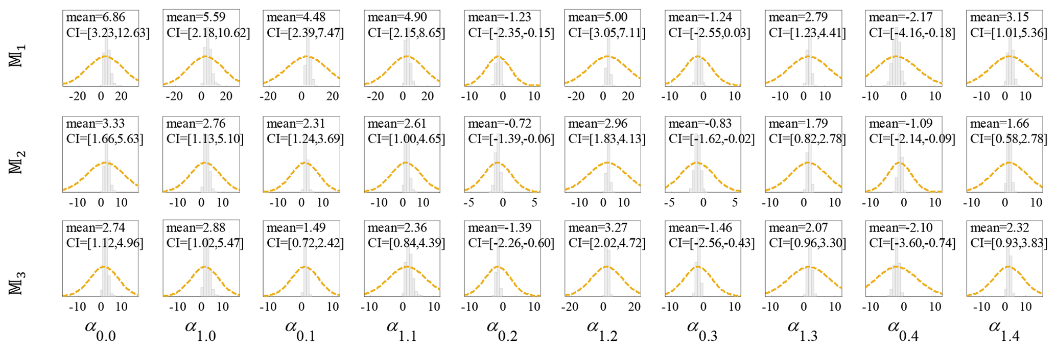
Figure F1 Distribution of the fragility model parameters ${\mathit{\theta }}_k=\left[{\left\{{\mathit{\alpha }}_{\mathrm{0},j},{\mathit{\alpha }}_{\mathrm{1},j}\right\}}_k,j=\mathrm{0}:\mathrm{4}\right]$ based on model class 𝕄_k (where $k=\mathrm{1}:\mathrm{3}$) for Class 1, brick masonry residential, South Pacific tsunami, by employing an adaptive MCMC procedure including samples drawn from the joint posterior PDF with their statistics (mean and COV) and the marginal normal priors (subfigures show the posterior statistics).