the Creative Commons Attribution 4.0 License.
the Creative Commons Attribution 4.0 License.
 | 15 May 2023
The role of preconditioning for extreme storm surges in the western Baltic Sea
Elin Andrée
Morten Andreas Dahl Larsen
Martin Stendel
Kristine Skovgaard Madsen
When natural hazards interact in compound events, they may reinforce each other. This is a concern today and in light of climate change. In the case of coastal flooding, sea-level variability due to tides, seasonal to inter-annual salinity and temperature variations, or larger–scale wind conditions modify the development and ramifications of extreme sea levels. Here, we explore how various prior conditions could have influenced peak water levels for the devastating coastal flooding event in the western Baltic Sea in 1872. We design numerical experiments by imposing a range of precondition circumstances as boundary conditions to numerical ocean model simulations. This allows us to quantify the changes in peak water levels that arise due to alternative preconditioning of the sea level before the storm surge. Our results show that certain preconditioning could have generated even more catastrophic impacts. As an example, a simulated increase in the water level of 36 cm compared to the 1872 event occurred in Køge just south of Copenhagen (Denmark) and surrounding areas – a region that was already severely impacted. The increased water levels caused by the alternative sea-level patterns propagate as long waves until encountering shallow and narrow straits, and after that, the effect vastly decreases. Adding artificial increases in wind speeds to each study point location reveals a near-linear relationship with peak water levels for all western Baltic locations, highlighting the need for good assessments of future wind extremes. Our research indicates that a more hybrid approach to analysing compound events and readjusting our present warning system to a more contextualised framework might provide a firmer foundation for climate adaptation and disaster risk management. In particular, accentuating the importance of compound preconditioning effects on the outcome of natural hazards may avoid under- or overestimation of the associated risks.
- Article
(5016 KB) - Full-text XML
- BibTeX
- EndNote


Several authors have recently demonstrated the importance of considering the compoundness of extreme events and suggested that such events may become more likely due to climate change (AghaKouchak et al., 2020; Santos et al., 2021; Vogel et al., 2021; Zscheischler et al., 2018). They include a range of natural hazards like floods and storms, the impacts of which may be enhanced or lessened by antecedent conditions that interact directly with the event, hence affecting the vulnerability of exposed areas (Bischiniotis et al., 2018; Bradstock et al., 2009; Johnson et al., 2016; McMillan et al., 2018; Raymond et al., 2020). The timescales of such “preconditioning” can vary from days to months or even years. For example, the exceptional 2018 European wildfire season that severely impacted northern Europe was preceded by above-average temperatures and abnormally dry (e.g. vegetation) conditions in most places, some extending back several months and some all the way back to 2017 (European Commission and Joint Research Centre, 2019). It was also generally exacerbated by unfavourable wind conditions and high temperatures during the summer. Compared to the average of 2008–2017, some countries like Norway, Sweden, Finland, Germany and the Czech Republic suffered a doubling or more of the number of recorded fires in 2018 (European Commission and Joint Research Centre, 2019). Similar examples involving different timescales include landslides that are predated by extensive soil erosion caused by, for example, rainfall or snowmelt (Hilker et al., 2009), as well as overland flooding induced by heavy rain that is exacerbated by falling on top of a very wet period, e.g. with saturated soils and filled water reservoirs (Hendry et al., 2019).
Management of the current and future risks of natural hazards often relies on learning and extrapolating from past extreme events, modelling, and climate change projections (Dangendorf et al., 2021; Frederikse et al., 2020; Harjanne et al., 2017; Travis and Bates, 2014). However, while the history of meteorological observations is long, modern-era instrumental measurements only date back to the founding of the first meteorological institutes in the latter part of the 19th century. As a result, comprehensive observations of low-probability high-impact events are generally scarce and limited to recent decades (Calafat and Marcos, 2020; Hallin et al., 2021; Jacobsen et al., 2021). In contrast, longer records include only the observed maxima, e.g. maximum observed water levels, inundation depths, precipitation intensities or wind speeds. Correspondingly, the extremes inferred from model simulations are mainly compared to observations in their ability to reconstruct maximum values and not their contexts (Marcos et al., 2015).
Storm surges and extreme sea levels are one of the main threats to people and properties along coastlines (Brown et al., 2018; Buchanan et al., 2017; Hallegatte et al., 2013; Vousdoukas et al., 2020; Wahl et al., 2017). Generally, high water levels are associated with low-pressure weather systems, resulting in strong winds piling seawater towards the shore and water levels exceeding the range of the astronomical tides. Wave-driven setup from waves breaking in the shallow surf zone may comprise 20 % to 30 % or more of the total surge during energetic wind conditions (Lavaud et al., 2020; Woodworth et al., 2019). However, the wind effect is only one of several drivers influencing high water levels' development, maximum elevation and duration. Other essential factors include sea-level variations due to tides (Arns et al., 2020), seasonal or inter-annual salinity and temperature variations, large-scale pressure fluctuations, dynamic water interactions with basin geometry and bathymetry (especially for marginal seas), and the initial distribution of seawater within a basin (Pugh, 1987). In combination, these factors can lead to both heightened and lowered surge levels.
Coastal flood risk assessments are generally based on local extreme sea-level statistics derived from time series of tide gauge measurements, with lengths varying from a few decades to more than 100 years. The extreme sea levels and their associated recurrence periods may be assessed using different variants of extreme value analysis on the observational records (Coles et al., 2001; Thorarinsdottir et al., 2017; Wahl et al., 2017). Similarly, future extreme sea-level statistics may be obtained by analysing modelled sea levels within a future time slice, e.g. 2071–2100, and contemporary scenario assumptions (Masson-Delmotte et al., 2021; Oppenheimer et al., 2019). It has been proposed that hydrodynamic models may be needed to refine flood risk assessments at regional to local scales. For example, Vousdoukas et al. (2016) suggest that by accounting for water-level attenuation due to land surface roughness, the estimated flood exposure decreases (inundation extent and depth) and hence also the estimated damages (Vafeidis et al., 2019). Likewise, several authors have recently addressed the potentially disproportional risks from compound coastal flooding, e.g. caused by a combination of storm surge and heavy rainfall (Bevacqua et al., 2019) or a surge combined with high river discharge (Couasnon et al., 2020), and the challenges for risk management concerning compound events in our study area (Modrakowski et al., 2022). Conversely, the role of preconditioning for the development of extreme sea levels has so far received less attention (Weisse and Weidemann, 2017).

Figure 1Map of the study area with a zoom-in on the Danish straits in the western Baltic Sea (a) and the entire Baltic Sea (b). Locations marked in the figure are mentioned in the text. Filled circles indicate locations of water-level measurements. This study focuses on the tide gauge locations marked in red.
As mentioned, the physical context is usually not considered in classical risk analysis, e.g. in calculations of statistical recurrence frequencies from observed annual maxima or other collections of extremes. Here we suggest that it is necessary to be able to “explain” the numbers and the associated uncertainty estimates to avoid under- or overestimation due to the compounded risks and, more generally, to improve confidence in the results of these kinds of studies for the benefit of adaptation planning. The motivation for this research is to address this research gap and investigate the potential influence of preconditioning of the Baltic Sea on an extreme wind-driven sea-level event in the western Baltic (Fig. 1).
The Baltic Sea is a marginal sea of the Atlantic Ocean characterised by complex coastlines. Its connection to the North Atlantic, via the North Sea and the shallow and narrow Danish straits, suppresses much of the sea-level variability coming from the North Atlantic. Instead, this flow restriction introduces other types of sea-level variability that may exacerbate extreme sea levels induced by storms. Atmospheric forcing can redistribute water between the different sub-basins in the Baltic or change the overall volume through water transport between the North and Baltic seas, which may cause the sea level to vary on timescales of weeks (Samuelsson and Stigebrandt, 1996; Weisse and Weidemann, 2017). Volume changes are commonly inferred from the water level at Landsort (Fig. 1b) because of its location close to the nodal line of the Baltic Sea, and it is referred to as the Baltic's filling level (Feistel et al., 2008; Lisitzin, 1974; Matthäus and Franck, 1992; Weisse and Weidemann, 2017). Likewise, oscillations related to the semi-enclosed nature of the Baltic Sea, known as seiches (Leppäranta and Myrberg, 2009; Pugh, 1987), contribute to sea-level variability. However, these are not yet fully understood (Weisse et al., 2021). The characteristic timescales for these oscillations have been estimated to be roughly equal to a day based on basin-wide (Wubber and Krauss, 1979), and sub-basin-wide (Jönsson et al., 2008) premises.
The importance of the contribution from filling levels and seiches to Baltic sea-level anomalies has previously been highlighted by Weisse and Weidemann (2017), who analysed sea-level data from a high-resolution tide-surge model driven by an atmospheric reanalysis. In their 64-year hindcast, high filling level (FL-H, defined as periods where the sea level near Landsort remains at least 15 cm above the local long-term mean for a minimum of 20 d; Mudersbach and Jensen, 2010) occurred on average 60 d per year. During these conditions, relatively lower wind speeds were needed to generate high sea levels. Weisse and Weidemann (2017) also showed that seiche contributions to peak water levels exceeded 10 cm in one-third of cases at the station Wismar on the German Baltic Sea coast.
For this study, we use a “storyline approach”, where we revisit the disastrous 1872 (western) Baltic Sea storm surge (Clemmensen et al., 2014; Colding, 1881; Rosenhagen and Bork, 2009), which stands as the worst storm surge on record experienced in the western Baltic Sea (Hallin et al., 2021). During this event, an unparalleled wind forcing from the northeasterly–easterly sector over a large expanse of the Baltic Sea (Rosenhagen and Bork, 2009) generated exceptional water levels, up to 3.5 m above average, affecting areas in Denmark, Germany and Sweden with catastrophic impacts (Colding, 1881; Hallin et al., 2021; Jacobsen et al., 2021). At least 271 persons drowned and about 15 000 lost their homes (Kiecksee et al., 1972; Petersen and Rohde, 1977). More than 400 sailing ships (15 Danish) and 23 steam ships became stranded or sank, mainly along the eastern shores of the Danish islands of Zealand and Falster (Bureau Veritas, 1872).
The main objective of our research is to answer the following question. What extreme water levels would have been obtained as a consequence of the 1872 storm if the antecedent conditions were different? We explore this research question using a set of numerical ocean model simulations that all arrive at states driven by the atmospheric conditions of the 1872 storm surge event. The differences between the simulations arise as we change the initial sea-level patterns (i.e. the prior conditions) of the simulations. This sensitivity test allows us to isolate the effects of preconditioning on extreme sea levels resulting from a specific storm. The regional atmospheric conditions during the 1872 storm have previously been reconstructed by Rosenhagen and Bork (2009) at the German national meteorological service Deutscher Wetterdienst (DWD). Their product yields higher maximum wind speeds that better agree with local observations than those generated in lower-resolution global reanalysis data (Feuchter et al., 2013). Here, the regional reconstruction is used as forcing for our simulations.
From historical records and modelling reconstructions of the storm surge event of 1872, it is evident that the Baltic Sea filling level in the weeks preceding 13 November 1872 was quite moderate. On this background – and given that the 1872 storm often serves as an absolute reference for, for example, climate change adaptation around the Baltic Sea – it is relevant to ask whether the 1872 storm is really the worst possible event that could have happened in the western Baltic. Since the filling level of the Baltic Sea exhibits natural variability with exceedances of the 1872 event, it is reasonable to assume that the initial filling level (serving as boundary conditions for the storm) could have been higher than it was (and lower as well, for that matter). To answer the above-mentioned question, we choose to replace the reconstructed filling level from 1872 with other physically consistent boundary conditions rather than artificially raising them by a factor, since local sea levels result from interactions between complex dynamical processes. While both methods generate synthetic events, which may be associated with a negligible probability, the former better supports our storyline approach, as it builds on real, historical events.
One of these events is the storm surge on 31 December 1904. For this storm, the pressure gradient in the western Baltic was about one-third larger than for the 1872 event. With easterly winds (rather than from the northeast as in 1872), water levels ran up to the “top five” at several locations in Denmark but remained well below the 1872 values (Jacobsen et al., 2021). Another event, which we use here as preconditioning, is a “silent storm surge” (i.e. a storm surge without a storm) of 4 January 2017 with high water levels, also among the top five at several locations (Jacobsen et al., 2021). This was due to a high water level in the days before the event. By definition, the observed combinations of wind and water levels during these previous events represent realistic conditions. While none are exact “scalings” of the 1872 event, we argue that our modifications are physically plausible, as they are well within the local range of natural variability. This extends to the question of the physical realism of the meteorological forcing scenarios, except for the transition within the model simulations (when we change from the preconditioning forcing data to those of the reconstructed 1872 event) – a transition that the model handles robustly.
In the following, we specifically compare the model simulations of 1872 with three alternative scenarios with more unfavourable preconditioning to quantify a range of implications of an “1872-like” storm. The substitute antecedent conditions are based on realistic simulations of contemporary sea-level events. In addition, we carry out a second set of simulations where we amplify the wind speeds used as input to the ocean model. These simulations aimed to assess the combined effect of storm and preconditioning enhancement on peak water levels.
Section 2 outlines the atmospheric conditions of the 1872 storm surge, the experimental design, the data sources and the ocean model setup. Section 3 presents our results and Sect. 4 the discussion and conclusions.
The following section describes the atmospheric conditions during the reference simulation, i.e. for the unperturbed simulation of the 1872 storm surge as reconstructed by our model system. We denote this as simulation O. Section 2.2 describes our three variant preconditioning scenarios, which we denote as experiment FL1, FL2 and S, and the physical conditions behind these cases. Section 2.3 describes the wind perturbation experiments, which are denoted by adding the percentual wind increase to the name of the experiment, e.g. “O + 20 %”, and Sect. 2.4 describes the model system.
2.1 Case study: the 1872 event
On 13 November 1872, catastrophic flooding took place along the southwestern Baltic Sea coasts (Fig. 1a). Water levels greatly surpassed previous records, and no flood event has even come close to the 1872 event since then. Water levels reached 3.38 m in Lübeck, 3.40 m in Travemünde and Eckernförde, 3.30 m in Kiel, 3.49 m in Schleswig, and 3.27 m in Flensburg (Petersen and Rohde, 1977). For Danish coastlines, Jacobsen et al. (2021) provide trend-free sea-level estimates based on the comprehensive collation of contemporaneous oceanic and atmospheric information by Colding (1881). Relative to the mean sea level in the year 2020, the water level reached 2.90 m at Køge and increased westward to more than 3.5 m by the Danish mainland (Jacobsen et al., 2021).
Unfavourable conditions for a storm surge are generated when westerlies transport large amounts of water through the Danish straits and into the Baltic Sea. A dangerous rise in the water level at the Baltic Sea coasts of Germany and Denmark can occur if the wind subsequently changes to a northeasterly direction. This mechanism was already discussed by Baensch (1875). Therefore, it is necessary to consider the atmospheric situation at least 2 weeks before the event when reconstructing the 1872 storm surge and similar events.
2.1.1 Atmospheric conditions
Between 1 and 11 November, low pressure was found over Scandinavia and the Norwegian Sea. Strong winds from westerly to southwesterly directions caused intense net transport of water through the Danish straits and into the Baltic Sea. The maximum cumulative transport at Cape Arkona on the island of Rügen occurred on 9 November (Rosenhagen and Bork, 2009). On 10 November, the weather pattern changed dramatically. A low crossed central Europe on quite an unusual track from northwest to southeast, while pressure rose sharply over Scandinavia. Consequently, the winds shifted from southwest to northeast, and the piled-up waters in the eastern Baltic Sea were released as a long wave travelling to the southwest. This situation – low pressure over central Europe, high pressure over Scandinavia and a maximum pressure gradient over the southwestern Baltic Sea – prevailed during the next 3 d, with both the high and the low intensifying further. On the morning of 13 November, the high over central Scandinavia had an unusually high sea-level pressure of 1047 hPa, whereas the low with a core pressure of 990 hPa was located over the border region of Saxony, Prussia and Bohemia. As a consequence, the northeasterly storm over the southwestern Baltic reached full gale force. With the weakening of both pressure centres, the strong winds died down, and water levels fell.
2.1.2 Data sources
The atmospheric conditions driving the development that culminated in the 1872 storm surge can be retrieved from a global reanalysis based on synoptic pressure observations (Compo et al., 2011). However, more local data are available than are included in global reanalyses. For our control simulation of the 1872 storm surge (denoted O), we therefore utilised two different sources of atmospheric forcing. First, to spin up the ocean model, we used forcing from the 20th Century Reanalysis in its most recent version 20CRv3 (Slivinski et al., 2019) for a simulation spanning the years 1871 to 1873. The 20CRv3 data set is available in 3-hourly resolution and 75 km grids (Slivinski et al., 2019) (https://psl.noaa.gov/data/gridded/data.20thC_ReanV3.html, last access: 1 December 2022). Second, we used a regional, gridded reconstruction with higher spatial (0.5 ∘ grids) and temporal (hourly) resolution (Rosenhagen and Bork, 2009) in the days preceding and during the storm surge event. This data set was supplied by the DWD. It is based on a more extensive set of observations and captures the very intense wind conditions during the event more accurately than the coarse, global reanalysis (Feuchter et al., 2013). For the analysis of the 1872 event, we have access to a substantial number of local and regional data, notably from Germany. Observations have also been preserved from other nations, many of which had already-established weather services. In Denmark, Niels Hoffmeyer reconstructed sea-level pressure fields from numerous observations that the Danish Meteorological Institute (DMI) had collected.
As pointed out in the previous section, one of the preconditions for the catastrophic flooding was the period of strong westerlies prior to the event that transported large amounts of water into the Baltic Sea. Therefore, the period from 1 to 14 November 1872 was considered in the reconstruction by Rosenhagen and Bork (2009), and the investigated area covered the northeast Atlantic and northern Europe as far east as the Baltic states. We used this data set when available, i.e. from 06:00 CET 1 November until the storm surge abated almost 2 weeks later.
The methods for generating the detailed 1872 atmospheric reconstruction are described in Rosenhagen and Bork (2009). Here, we give a brief overview of the concept behind the manipulation. Generally, we are interested in observations of sea-level pressure and wind direction and speed. From there, we can reconstruct the two-dimensional (geostrophic) wind fields that are required to run our ocean model. In practice, geostrophic wind fields can be determined by triangulation and compared to the wind observations. This construction is achieved by assuming an equilibrium between the Coriolis force and the pressure gradient force (Alexandersson et al., 1998). An extrapolation needs to be done to obtain winds at 10 m height, since the pressure fields have been reduced to sea level. Such extrapolations can be accomplished using empirical formulae. Many approaches have been suggested for this purpose, but common to them all is that they are quite dependent on the thermal layering of the lower troposphere, which we do not know. Further, this approach does not directly take into account frictional effects. Both factors can be approximated by using the distance from the sea, dependent on the wind direction.
2.2 Alternative preconditioning
To investigate scenarios of how altered antecedent conditions could have affected the development of the 1872 storm surge, we conducted three different experiments with alternative preconditioning. Two of the cases (FL1 and FL2) represent instances of high filling levels within the majority of the Baltic Sea. Case S incorporates a seiche effect. The data and methods for generating the scenarios are described in Sect. 2.2.1. The selection and physical conditions surrounding the instances are described in Sect. 2.2.3–2.2.4.
2.2.1 Scenario construction
As previously mentioned, the filling level of the Baltic Sea in November 1872 was fairly moderate. To demonstrate the implications for extreme sea levels if the Baltic had been preconditioned differently, we formed scenarios by imposing the atmospheric forcing of 1872 onto three alternative cases where the sea-level patterns were different (Fig. 2). The development of the Landsort water level for the respective simulations is shown in Fig. 3. In addition to showing the Landsort water level, Fig. 3 indicates the periods we use as preconditioning (i.e. alternative antecedent conditions) for the perturbed cases and the Landsort water levels corresponding to the snapshots in Fig. 2.
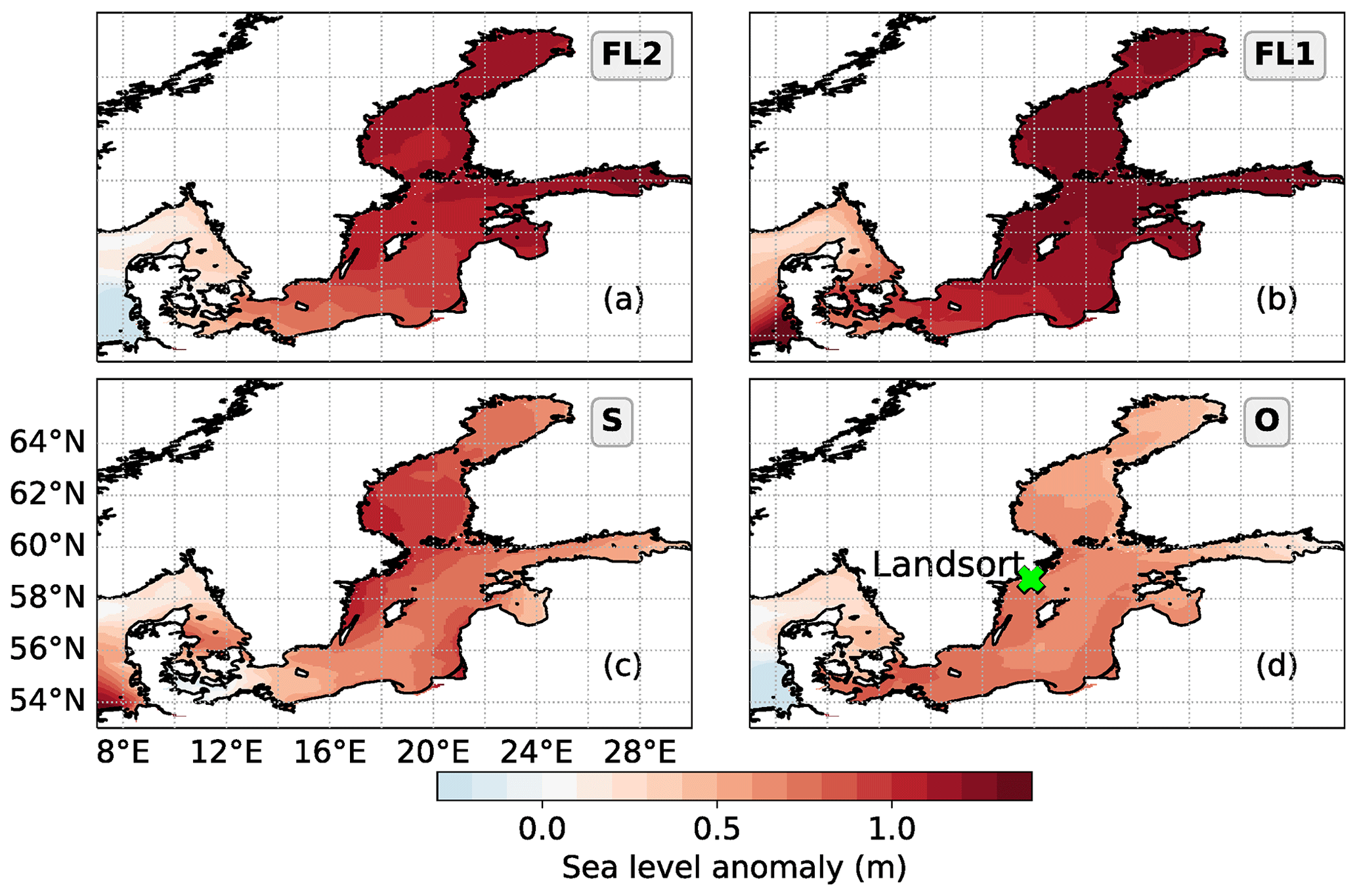
Figure 2The sea-level anomaly field that corresponds to the maximum water level at Landsort for each simulation (see Fig. 3 for time series). The magnitude of the sea-level anomalies is indicated by the colour bar. Panel (d) shows the unperturbed case (O) from 14:00 CET 11 November 1872. Preconditioning for the sea-level anomalies in panels (a) and (b) were obtained from an ocean hindcast (Andrée et al., 2021). The time is adjusted to match case O. Therefore, the time steps shown correspond to 9 November at 19:00 CET (FL2) and midnight (FL1), respectively. Case S (panel (c)) uses the same conditions as O, except that the atmospheric forcing between midnight on 9 November and up until 15:00 CET on 12 November 1872 is replaced by the corresponding times from 1 to 4 January 2017. The panel represents 04:00 CET on 12 November. Panel (d) shows the location of station Landsort, which is used to estimate the filling level.

Figure 3Preconditioning of the original (O) and alternative scenarios (FL2, FL1 and S) illustrated by the water level at station Landsort (lines). The dots show the Landsort water levels corresponding to the sea-level distributions in Fig. 2. Horizontal bars indicate the respective preconditioning periods; hashes indicate periods where the forcing in the alternative scenarios differs from that in O. See Sect. 2.2.1 for a description of the scenarios. The dotted bar indicates the period used to amplify the wind speed (see Sect. 2.3).
Scenarios FL1 and FL2 utilise monthly archived initial conditions from a regional ocean hindcast (Andrée et al., 2021). We forced the ocean model with the same regional reanalysis as the ocean hindcast (i.e. the Uncertainties in Ensembles of Regional Re-Analyses (UERRA) HARMONIE/V1 data set; Ridal et al., 2017) from the initialisation at the beginning of the respective month until the desired preconditioning state was reached (see Sect. 2.2.3–2.2.4). Horizontal bars in Fig. 3 mark these periods. The atmospheric forcing was thereafter switched directly to that of the high-resolution, 1872 reconstruction corresponding to 9 November. From then on and throughout the rest of the simulations, the atmospheric forcing that drives cases FL1 and FL2 is identical to the unperturbed (O) case. Differences in the dynamic development for each scenario are therefore solely due to perturbations of the initial state. The periods that utilise unperturbed atmospheric forcing from the 1872 event are indicated by solid colours (horizontal bars, Fig. 3). Case S is identical to O until midnight of 9 November 1872, when the forcing was switched to that of midnight of 1 January 2017. This forcing was utilised up until 15:00 CET on 4 January, when it was switched to the corresponding time from 12 November 1872. In effect, we replaced approximately 3.5 d of case O to incorporate a seiche effect in S.
2.2.2 Case FL2 – 13 March 1990
As a complement to using Landsort's water level, we did a spatial integration of sea-level anomalies eastward of 13 ∘ E to assess the Baltic's volume changes over time. The highest value corresponds to the Landsort maximum on 30 January 1983 and is described in Sect. 2.2.3 (case FL1). The second-highest event constitutes our case FL2, initialised on 13 March 1990.
The year 1990 started as unusually warm and was dominated by winds from southerly to westerly directions. Intense activity from low-pressure systems over the North Atlantic resulted in a succession of storms and frontal passages tracking over the North Sea. The strong zonal winds with intermittent episodes of northwesterly winds caused a net water transport into the Baltic Sea. From 21 February until 13 March, when case FL2 was initialised, the water level at Landsort steadily increased. Sea-level elevations were high overall but lower in the Bothnian Bay and Baltic Proper than in case FL1. The water level was exceptionally high also in the Gulf of Finland. Soomere and Pindsoo (2016) visualised modelled water levels above 80 cm near Tallinn for more than a week in March 1990.
2.2.3 Case FL1 – 1 February 1983
Case FL1 occurs in the aftermath of the highest observed water level at Landsort (Wolski et al., 2014). The atmospheric conditions leading up to this event constituted an extensive period of mild and wet weather with strong, zonal winds. The water level at Landsort started rising within the first few days of December. On 18 January, a low-pressure system that generated northwesterly, hurricane-strength winds along the Danish North Sea coastlines tracked from the north of the UK eastward towards the central Baltic Sea. During its passage, the relative water level at Landsort reached its highest observed value in an almost 136-year-long record. In the last week of January, southwesterly to westerly winds over the North Sea and the south to the central Baltic Sea were mainly between 10 and 20 m s−1. On 31 January, the Baltic Sea experienced winds of only a few metres per second, as a new low-pressure system was moving in over the northern UK. The wind-driven volume increase in the Baltic Sea generated persistent, elevated sea levels throughout most of the Baltic Sea (Fig. 2). The FL1 simulation was initialised from the state of the ocean at midnight on 1 February. At that time, the water level at Landsort had lowered slightly but remained exceptionally high (Fig. 3).
2.2.4 Case S – 4 January 2017
We constructed case S to incorporate the dynamics of a so-called silent surge event that impacted the western Baltic Sea in 2017 (She and Nielsen, 2019). The Danish Storm Council classified the silent surge as a 50-year event (i.e. 2 % or less chance of occurring in a given year) along Danish coastlines, despite only moderate and far-field wind forcing that was mainly distributed over the central Baltic Sea (She and Nielsen, 2019). A key component in this development was the preconditioning, with an elevated water level in the Baltic Sea and the Kattegat, in comparison to the southwestern Baltic Sea (She and Nielsen, 2019). This much more temporary and dynamic preconditioning is blended into case S.
Case S utilised the same atmospheric forcing and initial conditions as O, except for the period between midnight of 9 November and 15:00 CET on 12 November, which was replaced by midnight of 1 January to 15:00 CET on 4 January. This period was used to alter the preconditioning compared to O. Leading up to midnight of 9 November, southerly to southwesterly winds had piled up water in the northern Baltic Sea, generating a substantial sea-level gradient between the northern and southwestern ends. The onset of 1 January 2017 forcing started with northerly winds of around 10 m s−1 over the North Sea, southwesterly winds over the Baltic Proper and weaker northerly winds over the northern Baltic basins. Water that had been piled up in the Bothnian Bay had been released, and the wave energy was propagating southwards. The wind turned northwest, with around 10 m s−1 wind speeds over the Baltic and slightly higher over the North Sea. The wind field over the North Sea intensified and turned more westerly as a low-pressure system reached Norway. It tracked over the central Baltic Sea, following a southeasterly trajectory while generating northwesterly winds of around 20 m s−1 on its backside. At the forefront of the system, the southwesterly to easterly winds piled up water north- and westward. North of this low-pressure system, a high-pressure system intensified. This weather pattern generated northeasterly winds of about 20 m s−1 over the Baltic Sea along with northerly winds over Kattegat.
The atmospheric forcing that generated the 2017 surge continues to unfold for several hours after we switch back to the 1872 forcing (Sect. 2.2.1). In this way, the scenario captures the piling-up in the central Baltic Sea that sets the stage for the 2017 surge. It also captures the atmosphere's development into a persistent pressure distribution similar to 12 November 1872. From then on, we utilise the more intense and longer-lasting winds of 1872. In the observed development, relatively weaker northeasterly winds over the Baltic Sea persisted for some hours more, thereby adding to the severity of the 2017 surge.
2.3 Wind forcing amplification
In addition to the experiments detailed above, we conducted simulations of cases FL1, FL2 and O to amplify the wind forcing. These experiments aimed at illustrating whether changes in the wind forcing would generate feedback by either dampening or enhancing the influence of preconditioning in the perturbed scenarios relative to the control. We achieved this intensification of the wind forcing by increasing the wind speed by 20 % (FL1, FL2 and O) or 30 % (FL1 and FL2 only) in the atmospheric forcing, corresponding to 13 November 1872. This period is indicated by a dotted horizontal bar in Fig. 3.
2.4 Storm surge modelling
For the storm surge simulations, we used the regional 3D baroclinic ocean circulation model HIROMB-BOOS Model (HBM) for the North Sea and Baltic Sea (Berg and Poulsen, 2012; Kleine, 1994; She et al., 2007). For a detailed description see, for example, Berg and Poulsen (2012) and Poulsen and Berg (2012). HBM employs a two-way nesting scheme, allowing for the exchange of mass and momentum between the coarse and finer grids to resolve the complex flow structures of water exchange in the transition zone between the brackish Baltic Sea and the more saline North Sea. The coarse grid domain has a spatial resolution of 5.5 km and 50 vertical layers. The fine-grid domains are located in the German Bight and the inner Danish waters (transition zone between the North and Baltic Sea). They have 1.9 and 0.9 km spatial resolution with 24 and 52 vertical layers, respectively. We used climatological river runoff data obtained from the Hydrological Predictions for the Environment model for Europe (E-HYPE) (Donnelly et al., 2016). HBM has been used for a wide range of applications in, for example, climate and hindcast studies (Andrée et al., 2021; Fu et al., 2012; Madsen, 2009; Su et al., 2021; Tian et al., 2016) for assessing wind-driven sea-level sensitivity (Andrée et al., 2022) as well as for local marine management efforts of coastal estuaries (Murawski et al., 2021) and radioactive tracer studies (Lin et al., 2022). The present version was used for operational storm surge forecasting at the DMI between 2013 and 2018.
As already stated, we use case O as a reference simulation for the 1872 storm surge. The peak water levels obtained for this simulation agree with historical records within a few decimetres along the Danish coastlines but are overestimated by almost a metre at Travemünde. Overall, the results from case O confirm that the simulation is an appropriate point of departure for exploring alternative developments of the 1872 storm surge event.
Figure 2 shows the initial sea-level pattern in the Baltic Sea corresponding to the 1872 storm and the three alternative scenarios. As illustrated, cases FL2 and FL1 are characterised by overall increased volumes in the Baltic Sea. By contrast, case S is mainly characterised by a temporary piling-up of water in the Gulf of Bothnia. For both FL2 and FL1, the filling level is consistently higher than during the 1872 storm surge (O). Conversely, S is roughly similar in magnitude to O but exhibits a somewhat different sea-level pattern. Figure 3 shows the corresponding water levels measured at Landsort, which is often used to indicate the general Baltic Sea filling level (Feistel et al., 2008; Matthäus and Franck, 1992; Weisse and Weidemann, 2017). The timestamps on Fig. 3 are adjusted so that the development of cases FL2, FL1 and S matches that of the unperturbed event. As also shown in Fig. 2, cases FL2 and FL1 start with very high water levels at Landsort (Fig. 3) in comparison to the unperturbed event. At the end of the preconditioning period, the difference between these cases amounts to about 15 cm. This shift remains after the onset of the 1872 forcing (9 November), and very similar temporal patterns are displayed onward. This similarity can also be seen in case O regarding sub-daily oscillations. Cases FL2 and FL1 continued to be the highest throughout the event among the four cases presented here. The seiche event (case S) is identical to case O until the modification of the initial conditions on 9 November. Rather than the slow processes that bring about the high filling levels in cases FL2 and FL1 (Sect. 2.2.3–2.2.2), the preconditions for case S develop rapidly in just a little over a day. Even though the forcing only differs from case O for a few days, the water level reaches 27 cm higher at Landsort due to the characteristics of this preconditioning. The 1872 event, case O, maintains a Landsort water level of around 60 cm until the sharp decrease, shared by all events, during the night between 12–13 November. At the time of this drop in water level, the atmospheric forcing is identical for all cases, which results in nearly identical water-level reductions of 21 to 22 cm across all four cases.
Because of the connection between high water-level events in the western Baltic Sea and the associated filling level of the Baltic Sea in general (Weisse and Weidemann, 2017), we analysed the occurrence pattern between elevated sea levels and their corresponding duration for the entire observation period (1886–2021). For this analysis, we use Landsort observations available from the Swedish Meteorological and Hydrological Institute (SMHI, 2021) and dating back to 1886.

Figure 4Frequency of specific durations (1–14 d) for water levels of 40 to 70 cm. Panel (a) is for the entire period with observation data (1886–2021 – results provided per year), and panels (b)–(d) are for the specific events FL2, FL1 and S, respectively (results per event). Panels (b)–(d) have a similar y-axis range. Data are from the Swedish Meteorological and Hydrological Institute (SMHI) open data service (SMHI, 2021).
Specifically, we calculate the frequency with which certain elevated water levels occur (in 10 cm steps and aggregated to durations of 1–14 d). This analysis is performed on a yearly basis for the entire time series and per event for each of the events. As an example, a 3 d sea level of +60 cm occurs three times during FL2 and six times during FL1 but does not occur for event S (Fig. 4b–d). The same water-level threshold and duration occur on average 0.13 times per year (Fig. 4a).
From the empirical cumulative distribution function (not shown), we find that 99.0 % of the observations occur in the −50 to 50 cm interval and that 1-, 10- and 100-year return periods correspond to hourly water levels of approximately 75.7, 85.5 and 93.5 cm. Based on Fig. 4 and these return period statistics, the magnitude of water levels corresponding to FL1 and FL2 reflect relatively rare and extreme events, whereas event S is a high but not rare event. On this note, however, the 1-year return period level at Landsort accounts for 81 % of the 100-year return period level, keeping in mind the close relation to the general Baltic Sea filling level. Therefore, relatively high filling levels are seen at frequent intervals.
The freshwater content in the Baltic Sea means that there is a northward tilt of the sea level throughout the Baltic Sea. This characteristic results in a discrepancy between modelled values and observed relative water levels at Landsort, which is why we here choose not to reflect scenario preconditioning levels in terms of return period rates.
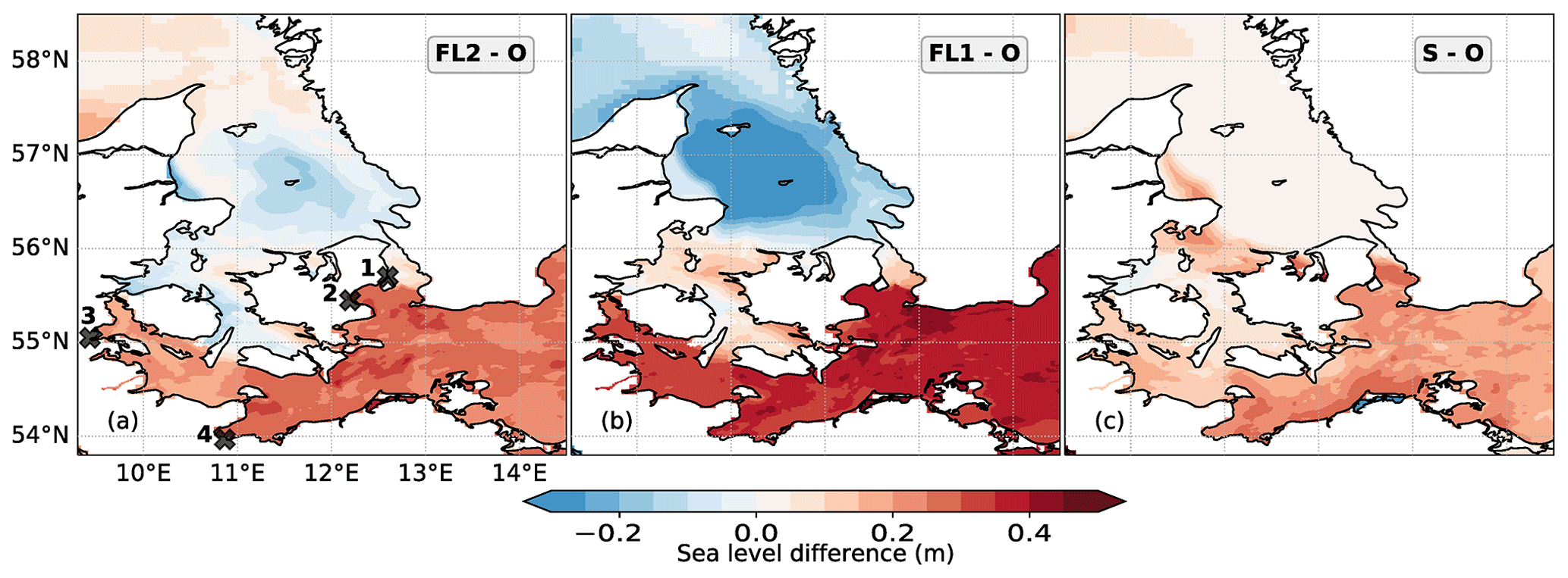
Figure 5The effect of alternative preconditioning on the 1872 storm surge. The panels show the difference between the maximum sea level obtained with alternative preconditioning and the maximum sea level obtained with the unperturbed preconditioning (O). The magnitude of the differences is indicated by the colour bar. Panel (a) shows the locations of København (Copenhagen, the Danish capital) (1), Køge (2), Aabenraa (3) and Travemünde (4).
Figure 5 shows the effect of the different preconditioning on the resulting maximum water levels in the western Baltic Sea. We subtracted the maximum values from the unperturbed case (O) from the maximums for cases FL2, FL1 and S to highlight spatial differences. The sea-level tilt between the northern- and easternmost basin ends versus the southern Baltic was most pronounced in the unperturbed representation. The maximum water level at Landsort occurred as the piled-up waters were released and propagated south and westwards, reducing the water level in the north and east and causing it to rise throughout the southwestern Baltic (Fig. 2d). The alternative preconditioning results in altered peak water levels throughout the southwestern Baltic Sea, as seen in Fig. 5. Of these, case FL1 results in the highest water levels by far. The peak water levels reach values in the general order of 0.3 to 0.45 m above the 1872 (case O) reference, with the largest differences seen as a piling-up south of the Swedish coastline, where the propagating waves encounter shallow depths. In a very narrow bay parallel to the German northeast coastline, the difference exceeds 0.5 m. In descending order, case FL1 is followed by case FL2 and case S, showing corresponding residuals relative to case O. FL2 results in values of 0.2 to 0.3 m and displays similar spatial patterns. For case S, on the other hand, differences of 0.25 to 0.3 m are mainly confined to the northeastern German coast, eastward of the narrow passageway between Germany and Denmark (Fehmarn Belt). One interesting feature of this case is that the signal of sea-level elevation extends into the sound, past the very shallow threshold (minimum depth of 8 m) separating Denmark's biggest island from Sweden. Up to 0.3 m higher water levels occur in the region of the Danish capital and Sweden's third-biggest city. For all cases, the three straits of Øresund, Storebælt and Lillebælt enforce drastically reduced residual levels, and the corresponding levels in Kattegat even show a negative amplitude for cases FL2 and FL1, with residual levels down to approximately −0.3 m for the latter of these.
Table 1Summary of the simulated peak water levels for the different experiments (Sect. 2). The unperturbed simulation (O) numbers are given in absolute values. For the remaining scenarios, the values shown indicate the difference to the unperturbed simulation (O's values subtracted). The Landsort column represents the maximum water level after 9 November (marked with dots in Fig. 3) and is included here for comparison. The experiments FL2, FL1 and S utilise the same atmospheric forcing as O but have different preconditioning. The scenarios denoted +20 % are the same as the respective O, FL2 and FL1, except that the wind speed was increased by 20 % on 13 November.
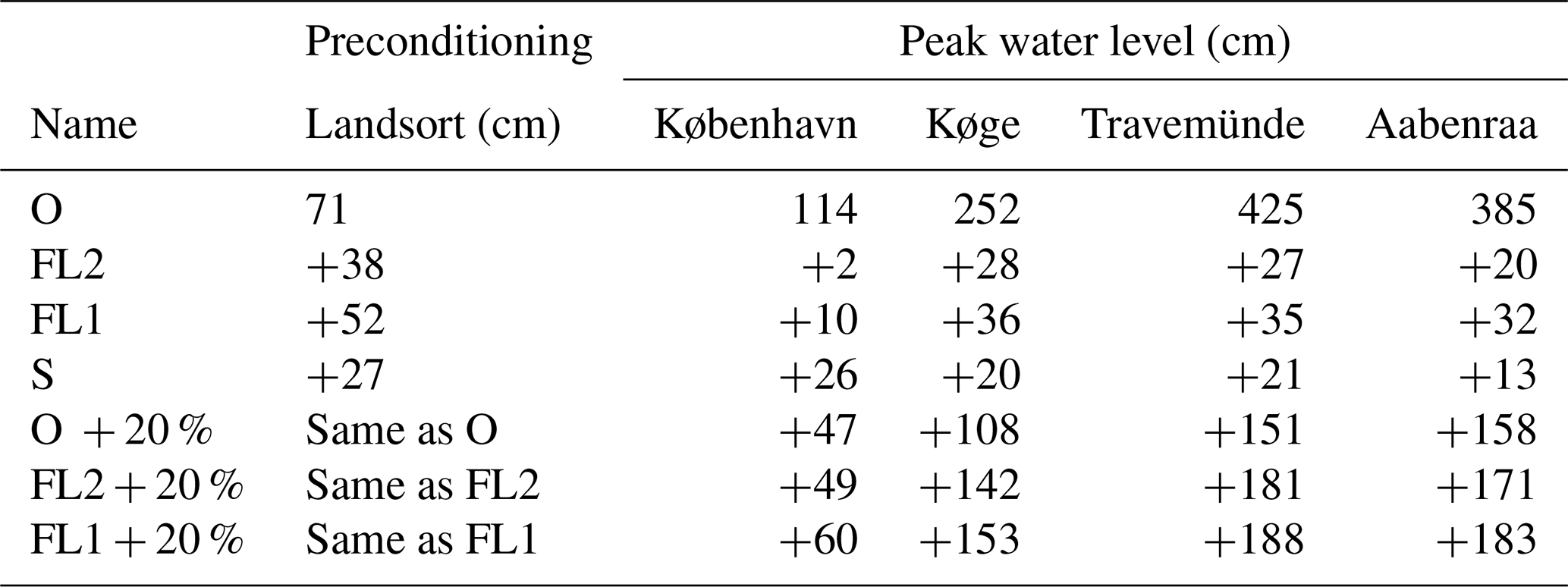
Table 2Time of the peak water levels reached (see Table 1). Absolute timestamps are retrieved from the unperturbed simulation (O). For the remaining scenarios, the values shown indicate the difference in minutes compared to the unperturbed simulation (O's timestamps subtracted).
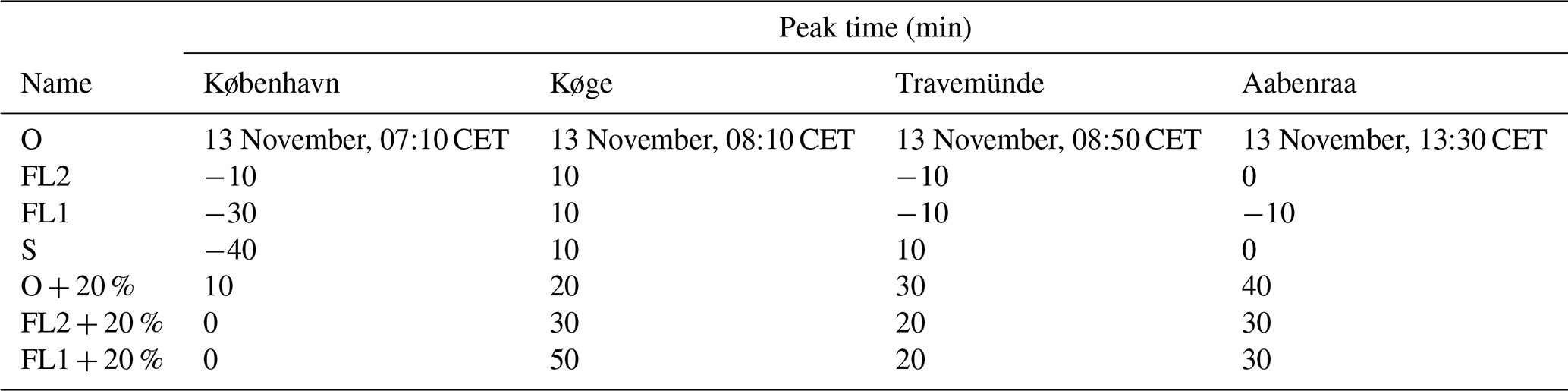
The maximum water levels (Table 1) and temporal water-level developments (Fig. 6) are shown for four different stations distributed around the western Baltic Sea (locations marked red in Fig. 1a). Referring to the O case, the timing of maximum levels occur within 1 h 40 min for København (Copenhagen), Køge and Travemünde (Table 2). In contrast, Aabenraa, located along the Jutland east coast in the westernmost part of the Baltic Sea, has a peak 6 h 20 min after København, which has the earliest of the other three peaks. The alternative preconditioning results in higher peak water levels, with differences ranging between 2 to 36 cm for all locations (Table 1). For comparison, the water level at Landsort was between 27 and 52 cm higher than O across the other scenarios. Between Køge and Copenhagen, the maximum water levels differ dramatically given the 30 km distance between them, with peak levels of 2.52 to 2.88 m for Køge and 1.14 to 1.40 m for Copenhagen (Table 1). Case FL1 exhibits the highest value for Køge, whereas case S is the highest for Copenhagen. In addition, Køge has a longer peak duration than Copenhagen. The fact that the Copenhagen time series is measured from the northern part of the city highly influences these results, as this location is located north of the shallow sill at the southern entrance of the sound. Therefore, these results mainly reflect inner-Copenhagen sea levels, whereas the suburbs of Copenhagen facing towards the south are likely to experience sea levels more comparable to those for Køge. Peak water levels for Aabenraa and Travemünde vary between 4.25 to 4.60 and 3.85 to 4.17 m, respectively, with the same order of cases as for Køge, whereas the peak duration to a higher degree resembles that of Copenhagen.
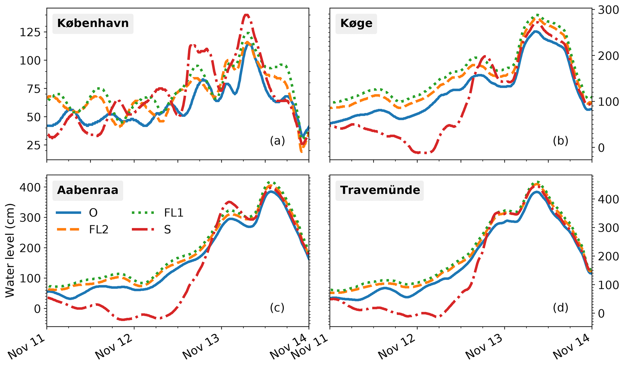
Figure 6The effect over time of alternative preconditioning for the 1872 storm surge. The panels show how the water levels develop over time for the unperturbed case (O) and the three alternative preconditioning scenarios (FL2, FL1 and S) at four different locations. Notice the differences in the y-axis scale.

Figure 7The effect of alternative preconditioning and wind speed intensification on peak water levels at four locations. The sea level's response to the amplified wind speed is strongly dependent on the model's wind-stress parameterisation and drag coefficient, as discussed in Andrée et al. (2022) for the same model. The experiments O, FL2, FL1 and S with an amplification factor of 1 are the same as in Fig. 6. In addition, experiments O, FL2 and FL1 were run with wind speeds multiplied by a factor of 1.2 or 1.3 for FL2 and FL1 only. The lines show linear fits to the peak water levels for FL2, FL1 and S, respectively (filled circles). Note the different scales on the y axes. See Sect. 2 for details on the respective intensification.
To investigate the combined effect of stronger winds and enhanced preconditioning for the 1872 event, we amplified the wind fields used to force the ocean simulations. The amplification was restricted to 13 November, and we used a fixed factor over the entire wind field. The results from intensifying the wind speed by 20 % (cases FL2, FL1 and O) and 30 % (cases FL2 and FL1) are shown in Fig. 7. Amplification of the wind speed resulted in increased peak water levels with an almost linear response (Fig. 7). This finding depends strongly on the model's wind-stress parameterisation and drag coefficient, which was discussed in Andrée et al. (2022) for idealised simulations with the same model. The linear response seems to indicate that, at least for the peak values, any dynamic changes to the sea-level patterns induced by the enhanced wind are marginal. At Copenhagen, 20 % wind speed amplification resulted in 40 % to 41 % (up to 0.5 m) higher water levels and 63 % to 65 % (up to almost 0.8 m) for a 30 % increase in the wind speed. Køge had a slightly higher response for 20 % wind speed increase (41 % to 43 %, up to 1.14 m) and lower for 30 % (61 % to 63 %, 1.76 m). Corresponding increases for Aabenraa reached 36 % to 41 % (up to 1.58 m) and 56 % to 58 % (2.33 m) and for Travemünde 33 % to 36 % (up to 1.54 cm) and 52 % to 53 % (2.38 m), respectively.
As shown in Table 2, the higher wind speeds delay the peak water levels in all cases and for all locations, while the preconditioning itself shifts the peak times both backwards and forwards in time.
In this paper, we quantify extreme water levels that may have been obtained as a consequence of the 1872 storm if the preconditioning was different. For this aim, we compared realistic model simulations of the 1872 storm surge with three alternative scenarios having more unfavourable preconditioning, drawn from reconstructions of contemporary sea-level events.
4.1 Effect of preconditioning
As shown in Table 1 and Figs. 5–6, the simulated extreme water levels for all three alternative scenarios overshoot the unperturbed values. When comparing S against FL2 and FL1, it is evident that the antecedent sea-level patterns also play a key role. The latter is also clearly seen from Fig. 6 regarding the local dynamics observed at København, Køge, Travemünde and Aabenraa. Depending on the exposed site of interest, our findings further suggest that the role of the preconditioning is crucial and that the effect is site-specific.
While this study intends to generate physically plausible scenarios, the way we modify the preconditions of the 1872 simulation by chaining together different physical events is purely synthetic. One could argue whether the combinations are physically conceivable, since they effectively represent unobserved events. All three of the cases FL2, FL1 and S could, however, be relevant in a climate change context.
Firstly, experiments FL2 and FL1 comprise high filling levels in the Baltic Sea. Figure 6 shows that the developments of these events are highly similar. Due to the higher filling level (14 m higher Landsort water level for FL1 than FL2), experiment FL1 results in higher peak water levels (Table 1). However, the difference is lower than the difference at Landsort. This discrepancy implies that the differences in peak water levels due to an increased volume in the Baltic Sea are not simple linear superpositions of the historic peak water levels and the volume difference as reflected by Landsort's filling level. An increased volume in the Baltic Sea will result from anthropogenic sea-level rise. Simply adding these drivers' contributions might overestimate the future peak water levels.
Secondly, experiment S demonstrates a scenario where an extra-tropical cyclone (ETC) precedes the 1872 event, similar to the 2017 storm surge event. Such successive events could become more common under the climate warming scenarios because of more frequent atmospheric blocking. Atmospheric blocking events are prevailing meteorological disturbances, commonly anti-cyclonic weather patterns, that deflect the large-scale westerly flow in the mid-latitudes (Barriopedro et al., 2006; Stendel et al., 2021; Woollings et al., 2018). Such flow-diversions can cause weather patterns to be blocked over a region, and the phenomenon is linked to various hydro-meteorological extremes (Rutgersson et al., 2022; Stendel et al., 2021). It has been proposed that atmospheric blocking events will occur more frequently in the future with climate change, particularly in the Northern Hemisphere (Nabizadeh et al., 2019). However, the understanding is hampered by the fact that climate models tend to underestimate the frequency of events (Zappa et al., 2014) and by a lack of knowledge of the feedback processes that may arise due to potential future changes in atmospheric dynamics (Stendel et al., 2021).
We have discussed different approaches to preconditioning and their effects on extreme water levels. By comparing the 1872 and 2017 floods, it is clear that wind speed is also an essential factor. So the question arises whether the 1872 storm with altered preconditioning would constitute a “worst-case event”. Two other storm events with a synoptic situation comparable to the 1872 event occurred in the 20th century. On 30–31 December 1904, the second-highest water level (1.43 m) for the period 1889–2007 was observed in Fredericia. In Travemünde (2.22 m) and Flensburg (2.33 m), high water levels were observed as well. On 30–31 December 1913, 9 years later, the highest recorded water level was recorded in Gedser. In Svendborg, water was 5 to 6 ft (1.5 to 1.8 m) and in Flensburg 2 m above normal. These events resemble the 1872 catastrophe, with strong westerlies followed by storms from the northeast. From these events, global reanalysis-based estimates of the pressure gradients in the region are larger than in 1872. In both cases (1904 and 1913), this situation persisted for only a couple of hours. In addition, the wind was from a slightly different direction, so not much damage was caused. However, a combination of the location and track of the 1872 low with pressure gradients of, for example, the 1904 low over a more extended period appears synoptically entirely possible. This would result in winds approximately 30 % stronger than in the 1872 case.
It is not clear whether such a situation would happen more frequently under climate change conditions (Stendel et al., 2021). As Scandinavian highs often occur in autumn and winter, strong lows moving eastward over northern Germany could initiate similar flooding events. With increasing temperatures, the atmosphere can bear more water vapour, so it appears possible that such a low could undergo vigorous development.
More speculatively, intense low-pressure systems originating from tropical cyclones have been observed over Great Britain. While this appears to have happened before (for example, the “great storm of 1703”), from a physical perspective, such events could be expected to happen more frequently in a warmer climate. There is, however, currently no indication in model simulations that such kinds of events will occur more frequently than in the past.
4.2 Implications for risk management
The 1872 storm surge was exceptional in both intensity and loss of lives and is by far the worst event documented in the western Baltic Sea by strong historical evidence (Hallin et al., 2021; Jacobsen et al., 2021). In this respect, the event has frequently been used as the benchmark worst-case scenario for coastal floods in the Baltic. However, given the results discussed above, one could argue for using even more extreme values from a physical perspective. While undoubtedly the severity of the 1872 storm was driven by high wind speeds (above 30 m s−1), we show here that the filling level of the Baltic Sea can add several decimetres more. Given that large parts of the coastal areas in the western Baltic are low-lying, this is a significant contribution. What remains is to quantify the present and future probability of such compound events. The 1872 storm surge has already been classified as a “low-probability, high impact event”, so these would be even more rare events. Speculatively, extrapolating from Fig. 6 would have resulted in approximately the same flood levels as in 1872 by “swapping” 5 % on the wind speed for optimal preconditioning, which perhaps would be more probable than the 1872 event itself.
Compared to 1872, the geography of the Baltic Sea region has significantly changed, and the number of people, assets and societal interests located along the coasts have increased as a result of general population growth and coastal urbanisation. Most of the major coastal cities along the Baltic Sea, including the low-lying capital region of Denmark that sits within the bottleneck passageway to the North Sea, have expanded in size and now critically rely on infrastructure that requires protection from seawater. Hence, the need for robust evidence on the risks of current and future storm surges has never been higher.
As mentioned above, extreme sea-level statistics based on tide gauge measurements or future projections of extreme sea levels currently generally comprise the “standard” for engineers and risk managers to cope with the accumulating climate risks due to storm surges and sea-level rise. Our research shows that a more hybrid approach, combining extreme sea-level statistics with state-of-the-art climate and ocean modelling, might be needed to understand the context of these extremes better. In this way, we can better account for the uncertainties and ensure a more robust platform for decision-making on climate change adaptation and disaster risk management. Such a hybrid approach could take the form displayed in this paper, where historical, well-described high-water-level events like the 1872 storm are revisited, and detailed numerical models are used to expand the uncertainty (e.g. by supplementing actual tide gauge measurements with perturbed model members) and to add to our physical understanding of how a combination of different factors lead to specific water levels.
4.3 Compound events under climate change and pre-warning system
As discussed previously, compound events, a combination of weather and climate extremes, are increasingly becoming a concern for many locations as the climate warms (AghaKouchak et al., 2020; Zscheischler et al., 2018). Those investigations, however, have not shed light on today's non-extreme events. The Intergovernmental Panel on Climate Change (IPCC) has identified one of the primary climate-change-related compound events as the consecutive occurrence of extreme or non-extreme events (IPCC, 2012). Climate change is altering storm surge events in our research area, and a non-extreme sea-level event today can have enormous consequences when it is paired with a subsequent, more severe storm surge event. As demonstrated by our results, a strong storm surge event in the western Baltic Sea area might have highly diverse effects depending on the initial filling conditions. However, our earlier attention was primarily drawn to the extreme cases, leaving the more common events largely under-researched (Weisse and Weidemann, 2017). Preconditioning and storm surge duration were found to be critical in this research. Thus, the current early warning system is challenged.
The local storm surge early warnings are a vital tool for reducing the impact of events on human activities and preventing economic loss in the face of global warming scenarios. The current storm surge warning system is based on a straightforward peak-over-threshold method, with the threshold increasing in tandem with the rise in mean sea level. The issue with the existing warning system is that it is difficult to contemplate storm surge events lasting over an extended period of time. As a result, non-extreme events are typically overlooked while developing an early warning system. We demonstrated that an early warning system should in principle consider far more time than the conventional forecast method now in use (5 d), i.e. to better account for the potential preconditioning of an extreme storm surge event. ECMWF began the operational application of medium-range forecasts (6–15 d) in 1979 (Bengtsson, 1985). With more than 40 years of experience, the medium-range forecast is becoming increasingly accurate, and recent advances in identifying the growing errors in the long-range forecast have contributed to enhance the operating system's predictability (Lillo and Parsons, 2017; Matsueda and Palmer, 2018). Our findings provide guidance for future developments of early warning systems. Indeed, it is easier to provide warnings for the longer-duration volume buildup in the Baltic Sea than for the shorter piling-up duration in experiment S. Early warnings for FL experiment situations that are well-designed allow for more time for planning and execution of hazard prevention and preparation measures.
Natural hazards and extreme events are contingent on the conditions before the event itself. However, historical records from before modern-era instrumental measurements often comprise only maximum values. Even when high-resolution observational or model products are available, it has long been the practice to assess the peak values without considering their context through the application of extreme value analysis. Perturbations of one or several of the constituents that together comprise a natural hazard allow for explorations of alternative scenarios to take the hazard context into account. This study focused on perturbations of the preconditioning of an exceptional storm surge event in the mouth of a semi-enclosed inland water body. The hazard is a high-impact, low-probability storm surge event that occurred in the western Baltic Sea in 1872. We generated alternative developments of the extreme sea-level hazard for this event by substituting the initial conditions. Here, we showed that alternative conditions could have further worsened the impacts by adding several decimetres to peak water levels. We suggest that a more hybrid approach of assessing the combined drivers and their contexts could provide a more robust foundation for climate adaptation and disaster risk management.
Furthermore, we find that the pressure gradient of this notorious storm has been exceeded by similar pressure patterns on at least two occasions during the 20th century, although these events have been shorter lasting. When adding artificial intensification of the wind speed, our simulations yield almost linear responses of further water-level increases throughout the western Baltic Sea, highlighting the need for good assessments of wind extremes.
We stress that understanding and awareness of preconditioning increases the actionable information before a natural hazard. Earlier warnings allow for more time for planning and executing hazard prevention and preparation efforts.
The HBM model codes used in this paper are available from Zenodo (https://doi.org/10.5281/zenodo.6769238, Su, 2022).
For access to the research data used in this paper, please contact the corresponding author.
EA: drafting of the paper and acquisition, analysis and interpretation of data. JS: acquisition, analysis and interpretation of data, editing of the paper. MADL, MS and MD: analysis and interpretation of data, editing of the paper. KSM, MD and MADL: project supervision. All authors contributed to the paper and approved the submitted version.
The contact author has declared that none of the authors has any competing interests.
Publisher's note: Copernicus Publications remains neutral with regard to jurisdictional claims in published maps and institutional affiliations.
This article is part of the special issue “Coastal hazards and hydro-meteorological extremes”. It is not associated with a conference.
Part of the funding was provided by the Danish State through the Danish Climate Atlas. A portion of the work was carried out within the “Extreme events in the coastal zone – a multidisciplinary approach for better preparedness” project, hosted by Uppsala University and funded by the Swedish Research Council, Formas.
This research has been supported by the Svenska Forskningsrådet Formas (grant no. 2018-01784).
This paper was edited by Joanna Staneva and reviewed by two anonymous referees.
AghaKouchak, A., Chiang, F., Huning, L. S., Love, C. A., Mallakpour, I., Mazdiyasni, O., Moftakhari, H., Papalexiou, S. M., Ragno, E., and Sadegh, M.: Climate extremes and compound hazards in a warming world, Annu. Rev. Earth Pl. Sc., 48, 519–548, 2020. a, b
Alexandersson, H., Schmith, T., Iden, K., and Tuomenvirta, H.: Long-term variations of the storm climate over NW Europe, The Global Atmosphere and Ocean System, 6, 97–120, 1998. a
Andrée, E., Su, J., Larsen, M. A. D., Madsen, K. S., and Drews, M.: Simulating major storm surge events in a complex coastal region, Ocean Model., 162, 101802, https://doi.org/10.1016/j.ocemod.2021.101802, 2021. a, b, c
Andrée, E., Drews, M., Su, J., Larsen, M. A. D., Drønen, N., and Madsen, K. S.: Simulating wind-driven extreme sea levels: Sensitivity to wind speed and direction, Weather and Climate Extremes, 36, 100422, https://doi.org/10.1016/j.wace.2022.100422, 2022. a, b, c
Arns, A., Wahl, T., Wolff, C., Vafeidis, A. T., Haigh, I. D., Woodworth, P., Niehüser, S., and Jensen, J.: Non-linear interaction modulates global extreme sea levels, coastal flood exposure, and impacts, Nat. Commun., 11, 1–9, 2020. a
Baensch, O.: Die Sturmfluth an den Ostsee-Küsten des Preussischen Staates vom 12./13. November 1872, Zeitschrift für Bauwesen, Berlin, 1875. a
Barriopedro, D., García-Herrera, R., Lupo, A. R., and Hernández, E.: A climatology of Northern Hemisphere blocking, J. Climate, 19, 1042–1063, 2006. a
Bengtsson, L.: Medium-range forecasting at the ECMWF, in: Advances in Geophysics, vol. 28, Elsevier, 3–54, https://doi.org/10.1016/S0065-2687(08)60184-3, 1985. a
Berg, P. and Poulsen, J. W.: Implementation details for HBM, in: DMI Technical Report 12-11, p. 147, DMI Copenhagen, https://www.dmi.dk/fileadmin/Rapporter/TR/tr12-11.pdf (last access: 1 December 2022), 2012. a, b
Bevacqua, E., Maraun, D., Vousdoukas, M. I., Voukouvalas, E., Vrac, M., Mentaschi, L., and Widmann, M.: Higher probability of compound flooding from precipitation and storm surge in Europe under anthropogenic climate change, Science Advances, 5, eaaw5531, https://doi.org/10.1126/sciadv.aaw5531, 2019. a
Bischiniotis, K., van den Hurk, B., Jongman, B., Coughlan de Perez, E., Veldkamp, T., de Moel, H., and Aerts, J.: The influence of antecedent conditions on flood risk in sub-Saharan Africa, Nat. Hazards Earth Syst. Sci., 18, 271–285, https://doi.org/10.5194/nhess-18-271-2018, 2018. a
Bradstock, R. A., Cohn, J. S., Gill, A. M., Bedward, M., and Lucas, C.: Prediction of the probability of large fires in the Sydney region of south-eastern Australia using fire weather, Int. J. Wildland Fire, 18, 932–943, https://doi.org/10.1071/WF08133, 2009. a
Brown, S., Nicholls, R. J., Goodwin, P., Haigh, I., Lincke, D., Vafeidis, A., and Hinkel, J.: Quantifying land and people exposed to sea-level rise with no mitigation and 1.5 ∘C and 2.0 ∘C rise in global temperatures to year 2300, Earths Future, 6, 583–600, 2018. a
Buchanan, M. K., Oppenheimer, M., and Kopp, R. E.: Amplification of flood frequencies with local sea level rise and emerging flood regimes, Environ. Res. Lett., 12, 064009, https://doi.org/10.1088/1748-9326/aa6cb3, 2017. a
Bureau Veritas: 44. Jahrgang (1872) Registre international de classification de navires, in: Deutsches Schiffahrtsmuseum Bremerhaven, vol. 44, Bureau Veritas, iSSN 11380883, http://www.digishelf.de/piresolver?id=54962810X (last access: 1 December 2022), 1872. a
Calafat, F. M. and Marcos, M.: Probabilistic reanalysis of storm surge extremes in Europe, P. Natl. Acad. Sci. USA, 117, 1877–1883, https://doi.org/10.1073/pnas.1913049117, 2020. a
Clemmensen, L. B., Bendixen, M., Hede, M. U., Kroon, A., Nielsen, L., and Murray, A. S.: Morphological records of storm floods exemplified by the impact of the 1872 Baltic storm on a sandy spit system in south-eastern Denmark, Earth Surf. Proc. Land., 39, 499–508, https://doi.org/10.1002/esp.3466, 2014. a
Colding, A.: Nogle Undersøgelser over Stormen over Nord- og Mellem-Europa af 12'te–14'de November 1872, Bianco Lunos Kgl. Hof-Bogtrykkeri, https://doi.org/10.48563/dtu-0000041, 1881. a, b, c
Coles, S., Bawa, J., Trenner, L., and Dorazio, P.: An introduction to statistical modeling of extreme values, vol. 208, Springer, ISBN 978-1-4471-3675-0, 2001. a
Compo, G. P., Whitaker, J. S., Sardeshmukh, P. D., Matsui, N., Allan, R. J., Yin, X., Gleason, B. E., Vose, R. S., Rutledge, G., Bessemoulin, P., Brönnimann, S., Brunet, M., Crouthamel, R. I., Grant, A. N., Groisman, P. Y., Jones, P. D., Kruk, M. C., Kruger, A. C., Marshall, G. J., Maugeri, M., Mok, H. Y., Nordli, Ø., Ross, T. F., Trigo, R. M., Wang, X. L., Woodruff, S. D., and Worley, S. J.: : The twentieth century reanalysis project, Q. J. Roy. Meteor. Soc., 137, 1–28, https://doi.org/10.1002/qj.776, 2011. a
Couasnon, A., Eilander, D., Muis, S., Veldkamp, T. I. E., Haigh, I. D., Wahl, T., Winsemius, H. C., and Ward, P. J.: Measuring compound flood potential from river discharge and storm surge extremes at the global scale, Nat. Hazards Earth Syst. Sci., 20, 489–504, https://doi.org/10.5194/nhess-20-489-2020, 2020. a
Dangendorf, S., Frederikse, T., Chafik, L., Klinck, J. M., Ezer, T., and Hamlington, B. D.: Data-driven reconstruction reveals large-scale ocean circulation control on coastal sea level, Nat. Clim. Change, 11, 514–520, https://doi.org/10.1038/s41558-021-01046-1, 2021. a
Donnelly, C., Andersson, J. C., and Arheimer, B.: Using flow signatures and catchment similarities to evaluate the E-HYPE multi-basin model across Europe, Hydrolog. Sci. J., 61, 255–273, https://doi.org/10.1080/02626667.2015.1027710, 2016. a
European Commission and Joint Research Centre, Gazzard, R., Müller, M., Sciunnach, R., Pecl, J., Konstantinov, V., Sbirnea, R., Cruz, M., Chassagne, F., Nugent, C., Benchikha, A., Kok, E., Gonschorek, A., Mharzi Alaoui, H., Maianti, P., Timovska, M., Zaken, A., Repšienė, S., Ascoli, D., Botnen, D., Leray, T., Libertà, G., Moffat, A., San-Miguel-Ayanz, J., Leisavnieks, E., Mitri, G., Pezzatti, B., Ruuska, R., Kaliger, A., Stoof, C., Fonzo, M., Beyeler, S., Oom, D., Eritsov, A., Maren, A., Pešut, I., Papageorgiou, K., Sandahl, L., Pfeiffer, H., Fresu, G., Debreceni, P., Longauerová, V., Sydorenko, S., Glazko, Z., Branco, A., Marzoli, M., Theodoridou, C., De Rigo, D., Jaunķiķis, Z., Ferrari, D., Durrant, T., Micillo, G., Piwnicki, J., Humer, F., Vivancos, T., Joannelle, P., Szczygieł, R., Pereira, T., Moreira, J., Vacik, H., Assali, F., Lopez-Santalla, A., Dursun, K., Petkoviček, S., Baltaci, U., Nuijten, D., Nagy, D., Jakša, J., Conedera, M., Abbas, M., Toumasis, I., Boca, R., and Mara, S.: Forest fires in Europe, Middle East and North Africa 2018, Publications Office of the European Union, https://doi.org/10.2760/561734, 2019. a, b
Feistel, R., Seifert, T., Feistel, S., Nausch, G., Bogdanska, B., Broman, B., Hansen, L., Holfort, J., Mohrholz, V., Schmager, G., Hagen, E., Perlet, I., and Wasmund, N.: Digital Supplement, chap. 20, John Wiley & Sons, Ltd, 625–667, https://doi.org/10.1002/9780470283134.ch20, 2008. a, b
Feuchter, D., Jörg, C., Rosenhagen, G., Auchmann, R., Martius, O., and Brönnimann, S.: The 1872 Baltic Sea storm surge, in: Weather extremes during the past 140 years, edited by: Brönnimann, S. and Martius, O., Geographica Bernensia G89, 91–98, https://doi.org/10.4480/GB2013.G89.10, 2013. a, b
Frederikse, T., Landerer, F., Caron, L., Adhikari, S., Parkes, D., Humphrey, V. W., Dangendorf, S., Hogarth, P., Zanna, L., Cheng, L., and Wu, Y.-H.: The causes of sea-level rise since 1900, Nature, 584, 393–397, https://doi.org/10.1038/s41586-020-2591-3, 2020. a
Fu, W., She, J., and Dobrynin, M.: A 20-year reanalysis experiment in the Baltic Sea using three-dimensional variational (3DVAR) method, Ocean Sci., 8, 827–844, https://doi.org/10.5194/os-8-827-2012, 2012. a
Hallegatte, S., Green, C., Nicholls, R. J., and Corfee-Morlot, J.: Future flood losses in major coastal cities, Nat. Clim. Change, 3, 802–806, https://doi.org/10.1038/nclimate1979, 2013. a
Hallin, C., Hofstede, J. L. A., Martinez, G., Jensen, J., Baron, N., Heimann, T., Kroon, A., Arns, A., Almström, B., Sørensen, P., and Larson, M. A: A Comparative Study of the Effects of the 1872 Storm and Coastal Flood Risk Management in Denmark, Germany, and Sweden, Water, 13, 1697, https://doi.org/10.3390/w13121697, 2021. a, b, c, d
Harjanne, A., Haavisto, R., Tuomenvirta, H., and Gregow, H.: Risk management perspective for climate service development – Results from a study on Finnish organizations, Adv. Sci. Res., 14, 293–304, https://doi.org/10.5194/asr-14-293-2017, 2017. a
Hendry, A., Haigh, I. D., Nicholls, R. J., Winter, H., Neal, R., Wahl, T., Joly-Laugel, A., and Darby, S. E.: Assessing the characteristics and drivers of compound flooding events around the UK coast, Hydrol. Earth Syst. Sci., 23, 3117–3139, https://doi.org/10.5194/hess-23-3117-2019, 2019. a
Hilker, N., Badoux, A., and Hegg, C.: The Swiss flood and landslide damage database 1972–2007, Nat. Hazards Earth Syst. Sci., 9, 913–925, https://doi.org/10.5194/nhess-9-913-2009, 2009. a
IPCC: Managing the Risks of Extreme Events and Disasters to Advance Climate Change Adaptation, in: A Special Report of Working Groups I and II of the Intergovernmental Panel on Climate Change, edited by: Field, C. B., Barros, V., Stocker, T. F., Qin, D., Dokken, D. J., Ebi, K. L., Mastrandrea, M. D., Mach, K. J., Plattner, G.-K., Allen, S. K., Tignor, M., and Midgley, P. M., Cambridge University Press, Cambridge, UK and New York, NY, USA, 582, https://www.ipcc.ch/report/managing-the-risks-of-extreme-events-and-disasters-to-advance (last access: 1 December 2022), 2012. a
Jacobsen, T., Sørensen, C., Woge Nielsen, J., and Su, J.: Historical extreme high water levels along the coastline of Denmark, DMI Report 21-28, Danish Meteorological Institute, Danish Coastal Authority, ISBN 978-87-7478-702-0, 2021. a, b, c, d, e, f, g
Johnson, F., White, C. J., van Dijk, A., Ekstrom, M., Evans, J. P., Jakob, D., Kiem, A. S., Leonard, M., Rouillard, A., and Westra, S.: Natural hazards in Australia: floods, Climatic Change, 139, 21–35, https://doi.org/10.1007/s10584-016-1689-y, 2016. a
Jönsson, B., Döös, K., Nycander, J., and Lundberg, P.: Standing waves in the Gulf of Finland and their relationship to the basin-wide Baltic seiches, J. Geophys. Res.-Oceans, 113, C03004, https://doi.org/10.1029/2006JC003862, 2008. a
Kiecksee, H., Thran, P., and Kruhl, H.: Die Ostsee-Sturmflut 1872: Heinz Kiecksee; mit einem Beitrag von P. Thran und H. Kruhl, Schriften des Deutschen Schiffahrtsmuseums, Westholsteinische Verlagsanstalt Boyens, ISBN 3-8042-0116-4, 1972. a
Kleine, E.: Das operationelle Modell des BSH für Nordsee und Ostsee: Konzeption und Übersicht, Bundesamt für Seeschiffahrt und Hydrographie, 1994. a
Lavaud, L., Bertin, X., Martins, K., Arnaud, G., and Bouin, M.-N.: The contribution of short-wave breaking to storm surges: The case Klaus in the Southern Bay of Biscay, Ocean Model., 156, 101710, https://doi.org/10.1016/j.ocemod.2020.101710, 2020. a
Leppäranta, M. and Myrberg, K.: Physical oceanography of the Baltic Sea, Springer Science & Business Media, ISBN 978-3-540-79703-6, 2009. a
Lillo, S. P. and Parsons, D. B.: Investigating the dynamics of error growth in ECMWF medium-range forecast busts, Q. J. Roy. Meteor. Soc., 143, 1211–1226, 2017. a
Lin, M., Qiao, J., Hou, X., Steier, P., Golser, R., Schmidt, M., Dellwig, O., Hansson, M., Örjan Bäck, Vartti, V.-P., Stedmon, C., She, J., Murawski, J., Aldahan, A., and Schmied, S. A.: Anthropogenic 236U and 233U in the Baltic Sea: Distributions, source terms, and budgets, Water Res., 210, 117987, https://doi.org/10.1016/j.watres.2021.117987, 2022. a
Lisitzin, E.: Seiches, in: Sea-Level Changes, Elsevier Oceanography Series, chap. 7, Elsevier, 185–196, https://doi.org/10.1016/S0422-9894(08)70781-5, 1974. a
Madsen, K. S.: Recent and future climatic changes in temperture, salinity, and sea level of the the North Sea and the Baltic Sea, PhD thesis, University of Copenhagen, ISBN 978-3-844-31270-6, 2009. a
Marcos, M., Calafat, F. M., Berihuete, Á., and Dangendorf, S.: Long-term variations in global sea level extremes, J. Geophys. Res.-Oceans, 120, 8115–8134, 2015. a
Masson-Delmotte, V., Zhai, P., Pirani, A., Connors, S. L., Péan, C., Berger, S., Caud, N., Chen, Y., Goldfarb, L., Gomis, M. I., Huang, M., Leitzell, K., Lonnoy, E., Matthews, J., Maycock, T. K., Waterfield, T. O., Yelekçi, R. Y., and Zhou, B. (Eds.): Climate Change 2021: The Physical Science Basis. Contribution of Working Group I to the Sixth Assessment Report of the Intergovernmental Panel on Climate Change, Summary for Policymakers, Cambridge University Press, in press, 2021. a
Matsueda, M. and Palmer, T.: Estimates of flow-dependent predictability of wintertime Euro-Atlantic weather regimes in medium-range forecasts, Q. J. Roy. Meteor. Soc., 144, 1012–1027, 2018. a
Matthäus, W. and Franck, H.: Characteristics of major Baltic inflows – a statistical analysis, Cont. Shelf Res., 12, 1375–1400, 1992. a, b
McMillan, S. K., Wilson, H. F., Tague, C. L., Hanes, D. M., Inamdar, S., Karwan, D. L., Loecke, T., Morrison, J., Murphy, S. F., and Vidon, P.: Before the storm: antecedent conditions as regulators of hydrologic and biogeochemical response to extreme climate events, Biogeochemistry, 141, 487–501, https://doi.org/10.1007/s10533-018-0482-6, 2018. a
Modrakowski, L.-C., Su, J., and Nielsen, A. B.: The Precautionary Principles of the Potential Risks of Compound Events in Danish Municipalities, Frontiers in Climate, 3, 772629, https://doi.org/10.3389/fclim.2021.772629, 2022. a
Mudersbach, C. and Jensen, J.: Küstenschutz an der Deutschen Ostseeküste, Zur Ermittlung von Eintrittswahrscheinlichkeiten extremer Sturmflutwasserstände, Korrespondenz Wasserwirtschaft, 3, 136–144, 2010. a
Murawski, J., She, J., Mohn, C., Frishfelds, V., and Nielsen, J. W.: Ocean Circulation Model Applications for the Estuary-Coastal-Open Sea Continuum, Frontiers in Marine Science, 8, 657720, https://doi.org/10.3389/fmars.2021.657720, 2021. a
Nabizadeh, E., Hassanzadeh, P., Yang, D., and Barnes, E. A.: Size of the Atmospheric Blocking Events: Scaling Law and Response to Climate Change, Geophys. Res. Lett., 46, 13488–13499, https://doi.org/10.1029/2019GL084863, 2019. a
Oppenheimer, M., Glavovic, B. C. Hinkel, J., van de Wal, R., Magnan, A. K., Abd-Elgawad, A., Cai, R., Cifuentes-Jara, M., DeConto, R. M., Ghosh, T., Hay, J., Isla, F., Marzeion, B., Meyssignac, B., and Sebesvari, Z.: Sea Level Rise and Implications for Low-Lying Islands, Coasts and Communities, in: IPCC Special Report on the Ocean and Cryosphere in a Changing Climate, edited by: Pörtner, H.-O., Roberts, D. C., Masson-Delmotte, V., Zhai, P., Tignor, M., Poloczanska, E., Mintenbeck, K., Alegría, A., Nicolai, M., Okem, A., Petzold, J., Rama, B., and and Weyer, N. M., Cambridge University Press, Cambridge, UK and New York, NY, USA, 321–445, https://doi.org/10.1017/9781009157964.006, 2019. Cambridge University Press, Cambridge, UK and New York, NY, USA, 321–445, https://doi.org/10.1017/9781009157964.006, 2019. a
Petersen, M. and Rohde, H.: Sturmflut: die grossen Fluten an den Küsten Schleswig-Holsteins und in der Elbe, Wachholtz, ISBN 978-3-529-06163-9, 1977. a, b
Poulsen, J. W. and Berg, P.: More details on HBM-general modelling theory and survey of recent studies, Tech. rep., Danish Meteorological Institute, 2012. a
Pugh, D. T.: Tides, surges and mean sea level, John Wiley and Sons Inc., New York, NY, ISBN 978-0-471-91505-8, 1987. a, b
Raymond, C., Horton, R. M., Zscheischler, J., Martius, O., AghaKouchak, A., Balch, J., Bowen, S. G., Camargo, S. J., Hess, J., Kornhuber, K., Oppenheimer, M., Ruane, A. C., Wahl, T., and White, K.: Understanding and managing connected extreme events, Nat. Clim. Change, 10, 611–621, https://doi.org/10.1038/s41558-020-0790-4, 2020. a
Ridal, M., Olsson, E., Unden, P., Zimmermann, K., and Ohlsson, A.: Uncertainties in Ensembles of Regional Re-Analyses-Deliverable D2.7 HARMONIE reanalysis report of results and dataset, Tech. rep., Swedish Meteorological and Hydrological Institute, http://www.uerra.eu/publications/deliverable-reports.html (last access: 30 June 2021), 2017. a
Rosenhagen, G. and Bork, I.: Rekonstruktion der Sturmwetterlage vom 13. November 1872, Küste, 75, 51–70, 2009. a, b, c, d, e, f, g
Rutgersson, A., Kjellström, E., Haapala, J., Stendel, M., Danilovich, I., Drews, M., Jylhä, K., Kujala, P., Larsén, X. G., Halsnæs, K., Lehtonen, I., Luomaranta, A., Nilsson, E., Olsson, T., Särkkä, J., Tuomi, L., and Wasmund, N.: Natural hazards and extreme events in the Baltic Sea region, Earth Syst. Dynam., 13, 251–301, https://doi.org/10.5194/esd-13-251-2022, 2022. a
Samuelsson, M. and Stigebrandt, A.: Main characteristics of the long-term sea level variability in the Baltic Sea, Tellus A, 48, 672–683, 1996. a
Santos, V. M., Casas-Prat, M., Poschlod, B., Ragno, E., van den Hurk, B., Hao, Z., Kalmár, T., Zhu, L., and Najafi, H.: Statistical modelling and climate variability of compound surge and precipitation events in a managed water system: a case study in the Netherlands, Hydrol. Earth Syst. Sci., 25, 3595–3615, https://doi.org/10.5194/hess-25-3595-2021, 2021. a
She, J. and Nielsen, J. W.: 'Silent' storm surge extremes in the western Baltic Sea on 4 January 2017, J. Oper. Oceanogr., 12, S111–S116, 2019. a, b, c
She, J., Berg, P., and Berg, J.: Bathymetry impacts on water exchange modelling through the Danish Straits, J. Marine Syst., 65, 450–459, 2007. a
Slivinski, L. C., Compo, G. P., Whitaker, J. S., Sardeshmukh, P. D., Giese, B. S., McColl, C., Allan, R., Yin, X., Vose, R., Titchner, H., Kennedy, J., Spencer, L. J., Ashcroft, L., Brönnimann, S., Brunet, M., Camuffo, D., Cornes, R., Cram, T. A., Crouthamel, R., Domínguez-Castro, F., Freeman, J. E., Gergis, J., Hawkins, E., Jones, P. D., Jourdain, S., Kaplan, A., Kubota, H., Le Blancq, F., Lee, T. C., Lorrey, A., Luterbacher, J., Maugeri, M., Mock, C. J., Moore, G. W. K., Przybylak, R., Pudmenzky, C., Reason, C., Slonosky, V. C., Smith, C. A., Tinz, B., Trewin, B., Valente, M. A., Wang, X. L., Wilkinson, C., Wood, K., and Wyszyński, P.: Towards a more reliable historical reanalysis: Improvements for version 3 of the Twentieth Century Reanalysis system, Q. J. Roy. Meteor. Soc., 145, 2876–2908, 2019. a, b
SMHI: SMHI Open Data: The national archive for oceanographic data, Swedish Meteorological and Hydrological Institute [data set], https://www.smhi.se/data/oceanografi/ladda-ner-oceanografiska-observationer#param=sealevelrh2000,stations=all,stationid=207 (last access: 1 December 2022), 2021. a, b
Soomere, T. and Pindsoo, K.: Spatial variability in the trends in extreme storm surges and weekly-scale high water levels in the eastern Baltic Sea, Cont. Shelf Res., 115, 53–64, 2016. a
Stendel, M., Francis, J., White, R., Williams, P. D., and Woollings, T.: Chapter 15 – The jet stream and climate change, Climate Change, 2021, 327–357, https://doi.org/10.1016/B978-0-12-821575-3.00015-3, 2021. a, b, c, d
Su, J.: HBM DKSS version 2013 (DKSS-2013), Zenodo [code], https://doi.org/10.5281/zenodo.6769238, 2022. a
Su, J., Andrée, E., Nielsen, J. W., Olsen, S. M., and Madsen, K. S.: Sea Level Projections From IPCC Special Report on the Ocean and Cryosphere Call for a New Climate Adaptation Strategy in the Skagerrak-Kattegat Seas, Front. Mar. Sci., 8, 629470, https://doi.org/10.3389/fmars.2021.629470, 2021. a
Thorarinsdottir, T. L., Guttorp, P., Drews, M., Kaspersen, P. S., and de Bruin, K.: Sea level adaptation decisions under uncertainty, Water Resour. Res., 53, 8147–8163, https://doi.org/10.1002/2016WR020354, 2017. a
Tian, T., Su, J., Boberg, F., Yang, S., and Schmith, T.: Estimating uncertainty caused by ocean heat transport to the North Sea: experiments downscaling EC-Earth, Clim. Dynam., 46, 99–110, https://doi.org/10.1007/s00382-015-2571-8, 2016. a
Travis, W. R. and Bates, B.: What is climate risk management?, Climate Risk Management, 1, 1–4, https://doi.org/10.1016/j.crm.2014.02.003, 2014. a
Vafeidis, A. T., Schuerch, M., Wolff, C., Spencer, T., Merkens, J. L., Hinkel, J., Lincke, D., Brown, S., and Nicholls, R. J.: Water-level attenuation in global-scale assessments of exposure to coastal flooding: a sensitivity analysis, Nat. Hazards Earth Syst. Sci., 19, 973–984, https://doi.org/10.5194/nhess-19-973-2019, 2019. a
Vogel, J., Paton, E., Aich, V., and Bronstert, A.: Increasing compound warm spells and droughts in the Mediterranean Basin, Weather and Climate Extremes, 32, 100312, https://doi.org/10.1016/j.wace.2021.100312, 2021. a
Vousdoukas, M. I., Voukouvalas, E., Mentaschi, L., Dottori, F., Giardino, A., Bouziotas, D., Bianchi, A., Salamon, P., and Feyen, L.: Developments in large-scale coastal flood hazard mapping, Nat. Hazards Earth Syst. Sci., 16, 1841–1853, https://doi.org/10.5194/nhess-16-1841-2016, 2016. a
Vousdoukas, M. I., Mentaschi, L., Hinkel, J., Ward, P. J., Mongelli, I., Ciscar, J.-C., and Feyen, L.: Economic motivation for raising coastal flood defenses in Europe, Nat. Commun., 11, 1–11, 2020. a
Wahl, T., Haigh, I. D., Nicholls, R. J., Arns, A., Dangendorf, S., Hinkel, J., and Slangen, A. B. A.: Understanding extreme sea levels for broad-scale coastal impact and adaptation analysis, Nat. Commun., 8, 16075, https://doi.org/10.1038/ncomms16075, 2017. a, b
Weisse, R. and Weidemann, H.: Baltic Sea extreme sea levels 1948–2011: Contributions from atmospheric forcing, Proc. IUTAM, 25, 65–69, https://doi.org/10.1016/j.piutam.2017.09.010, 2017. a, b, c, d, e, f, g, h
Weisse, R., Dailidienė, I., Hünicke, B., Kahma, K., Madsen, K., Omstedt, A., Parnell, K., Schöne, T., Soomere, T., Zhang, W., and Zorita, E.: Sea level dynamics and coastal erosion in the Baltic Sea region, Earth Syst. Dynam., 12, 871–898, https://doi.org/10.5194/esd-12-871-2021, 2021. a
Wolski, T., Wiśniewski, B., Giza, A., Kowalewska-Kalkowska, H., Boman, H., Grabbi-Kaiv, S., Hammarklint, T., Holfort, J., and Lydeikaitė, Ž.: Extreme sea levels at selected stations on the Baltic Sea coast, Oceanologia, 56, 259–290, https://doi.org/10.5697/oc.56-2.259, 2014. a
Woodworth, P. L., Melet, A., Marcos, M., Ray, R. D., Wöppelmann, G., Sasaki, Y. N., Cirano, M., Hibbert, A., Huthnance, J. M., Monserrat, S., and Merrifield, M. A.: Forcing factors affecting sea level changes at the coast, Surv. Geophys., 40, 1351–1397, 2019. a
Woollings, T., Barriopedro, D., Methven, J., Son, S.-W., Martius, O., Harvey, B., Sillmann, J., Lupo, A. R., and Seneviratne, S.: Blocking and its response to climate change, Current Climate Change Reports, 4, 287–300, 2018. a
Wubber, C. and Krauss, W.: The two dimensional seiches of the Baltic Sea, Oceanol. Acta, 2, 435–446, 1979. a
Zappa, G., Masato, G., Shaffrey, L., Woollings, T., and Hodges, K.: Linking Northern Hemisphere blocking and storm track biases in the CMIP5 climate models, Geophys. Res. Lett., 41, 135–139, 2014. a
Zscheischler, J., Westra, S., Van Den Hurk, B. J., Seneviratne, S. I., Ward, P. J., Pitman, A., AghaKouchak, A., Bresch, D. N., Leonard, M., Wahl, T., and Zhang, X. B.: Future climate risk from compound events, Nat. Clim. Change, 8, 469–477, 2018. a, b