Pseudo-prospective testing of 5-year earthquake forecasts for California using inlabru

Probabilistic earthquake forecasts estimate the likelihood of future earthquakes within a specified time-space-magnitude window and are important because they inform planning of hazard mitigation activities on different time scales. The spatial component of such forecasts, expressed as seismicity models, generally relies upon some combination of past event locations and underlying factors which might affect spatial intensity, such as strain rate, fault location and slip rate or past seismicity. For the first time, we extend previously reported spatial seismicity models, generated using the open source inlabru package, to time-independent earthquake forecasts using California as a case study. The inlabru approach allows the rapid evaluation of point process models which integrate different spatial datasets. We explore how well various candidate forecasts perform compared to observed activity over three contiguous 5-year time periods using the same training window for the input seismicity data. In each case we compare models constructed from both full and declustered earthquake catalogues. In doing this, we compare the use of synthetic catalogue forecasts to the more widely used grid-based approach of previous forecast testing experiments. The simulated catalogue approach uses the full model posteriors to create Bayesian earthquake forecasts, not just the mean. We show that simulated catalogue based forecasts perform better than the grid-based equivalents due to (a) their ability to capture more uncertainty in the model components and (b) the associated relaxation of the Poisson assumption in testing. We demonstrate that the inlabru models perform well overall over various time periods: The full catalogue models perform favourably in the first testing period (2006–2011) while the declustered catalogue models perform better in the 2011–2016 testing period, with both sets of models performing less well in the most recent (2016–2021) testing period. Together, these findings demonstrate a significant improvement in earthquake forecasting is possible although this has yet to be tested and proven in true prospective mode.

1 Introduction

Probabilistic earthquake forecasts represent our best understanding of the expected occurrence of future seismicity (Jordan and Jones, 2010). Developing demonstratively robust and reliable forecasts is therefore a key goal for seismologists. A key component of such forecasts, regardless of the timescale in question, is a reliable spatial seismicity model that incorporates as much useful spatial information as possible in order to identify areas at risk. For example in probabilistic seismic hazard modelling (PSHA) a time-independent spatial seismicity model is developed by combining a spatial model for the seismic sources with a frequency magnitude distribution. In light of the ever-growing abundance of earthquake data and the presence of spatial information that might help understand patterns of seismicity, Bayliss et al. (2020) developed a spatially varying point process model for spatial seismicity using log-Gaussian Cox processes evaluated with the Bayesian integrated nested Laplace approximation method (Rue et al., 2009) implemented with the open-source R package inlabru (Bachl et al., 2019). Time-independent earthquake forecasts require not only an understanding of spatial seismicity, but also need to prove themselves to be consistent with observed event rates and earthquake magnitudes in the future.

Forecasts can only be considered meaningful if they can be shown to demonstrate a degree of proficiency at describing what future seismicity might look like. The Regional Earthquake Likelihood Model (RELM, Field, 2007) experiment and subsequent collaboratory for the study of earthquake predictability (CSEP) experiments challenged forecasters to construct earthquake forecasts for California, Italy, New Zealand and Japan (e.g. Schorlemmer et al., 2018; Taroni et al., 2018; Rhoades et al., 2018, and other articles in this special issue) to be tested in prospective mode using a suite of predetermined statistical tests. The testing experiments found that the best performing model for seismicity in California was the Helmstetter et al. (2007) smoothed seismicity model, whether aftershocks were included or not (Zechar et al., 2013). This model requires no mosaic of seismic source zones to be constructed, requiring only one free parameter, the spatial dimension of the smoothing kernel. In the years since this experiment originally took place, there has been considerable work both to improve the testing protocols and to develop new forecast models which may improve upon the performance of the data-driven Helmstetter et al. (2007) model, primarily by including different types of spatial information to augment what can be inferred from the seismicity alone. Multiplicative hybrid models (Marzocchi et al., 2012; Rhoades et al., 2014, 2015) have shown some promise, but these require some care in construction and further testing is needed (Bayona et al., 2022). The performance of smoothed seismicity models has been found to be inconsistent in testing outside of California, e.g. with the Italian CSEP experiment finding smoothed past seismicity alone did not do as well as models with much longer term seismicity and fault information (Taroni et al., 2018). Thus, finding and testing new methods of allowing different data types to be easily included in developing a forecast model is an important research goal. Here we explore in particular the role of testing an ensemble of point process simulated catalogues (Savran et al., 2020) in comparison with traditional grid-based tests, where the underlying point process is locally averaged in a grid element.

In this paper we construct and test a series of time-independent forecasts for California by building on the spatial modelling approach described by Bayliss et al. (2020). As a first step in the modelling we take a pseudo-prospective approach to model design, with the forecasts being tested retrospectively on time periods subsequent to the data on which they were originally constructed, and test the models' performance against actual outcome using the pyCSEP package (Savran et al., 2021, 2022). This is not a sufficient criterion for evaluating forecast power in true prospective mode, but is a necessary step on the way, and (given similar experience of hindcasting in cognate disciplines such as meteorology) can inform the development of better real-time forecasting models. The results presented here will in due course be updated and tested in true prospective mode, using a training dataset up to the present. We first test the pseudo-prospective seismicity forecasts in a manner consistent with the RELM evaluations. For this comparison we use a grid of event rates and the same training and testing time windows to provide a direct comparison to the forecasts of the smoothed seismicity models of Helmstetter et al. (2007), which use seismicity data alone as an input, and provide a suitable benchmark for our study. We then extend this approach to the updated CSEP evaluations for simulated catalogue forecasts (Savran et al., 2020) and show that the synthetic catalogue-based forecasts perform better than the grid-based equivalents, due to their ability to capture more uncertainty in the model components and the relaxation of the Poisson assumption in testing.

2 Method

We develop a series of spatial models of seismicity modelled by a time-independent log-Gaussian Cox process and fitted with inlabru. This process is summarized in the workflow in Fig. 1, which describes the steps involved in constructing an inlabru model, and takes the reader through the process from data to forecasts so that an independent researcher can reproduce the method presented here. The models take as input 20 years (1985–2005) of California earthquakes with magnitude ≥4.95 from the UCERF3 dataset (Field et al., 2014), with the magnitude cut-off chosen to be consistent with the RELM forecast criteria. The locations of these events are an intrinsic component of a point process model with spatially varying intensity λ(s), where the intensity is described as a function of some underlying spatial covariates x_m(s), e.g. input data from seismicity catalogues or geodetic observations of strain rate, and a Gaussian random field ζ(s) to account for spatial structure that is not explained by the model covariates. The spatially varying intensity can then be described with a linear predictor η(s) such that

$$\begin{array}{}\text{(1)}& \mathit{\lambda }\left(\mathbf{s}\right)=e^{\mathit{\eta }\left(\mathbf{s}\right)},\end{array}$$

and η(s) can be broken down into a sum of linearly combined components:

$$\begin{array}{}\text{(2)}& \mathit{\eta }\left(\mathbf{s}\right)={\mathit{\beta }}_{\mathrm{0}}+\sum _{m=\mathrm{1}}^M{\mathit{\beta }}_{\mathrm{m}}{x}_m\left(\mathbf{s}\right)+\mathit{\zeta }\left(\mathbf{s}\right).\end{array}$$

The β₀ term is an intercept term, which would describe a spatially homogeneous Poisson intensity if no other components were included, and each β_m describes the weighting of individual spatial components in the model. β₀ is essentially the uniform average or base level intensity, which allows the possibility of earthquakes happening over all of the region of interest as a null hypothesis, so “surprises” are possible, although unlikely after adding the other terms and renormalising. The models are built on a mesh (step 2 of Fig. 1) which is required to perform numerical integration in the spatial domain, with the model intensity evaluated at each mesh vertex as a function of the random field (RF, which is mapped by stochastic partial differential equations or SPDE in step 3 of Fig. 1) and other components of the linear predictor function (Eq. 2). Fitting the model with integrated nested Laplace approximations using inlabru results in a posterior probability distribution for each of the model component weights, the random field and the joint posterior probability distribution for the intensity as a function of these components. The expected number of events can then be approximated by summing over the mesh and associated weights over the area of interest (Step 5 of Fig. 1). The performance of the models can then be evaluated by comparing the expected versus the observed number of events, and the models ranked using the resulting model deviance information criterion (DIC). The DIC is commonly used in other applications of Bayesian inference, including inlabru applications to other problems, such as spatial distributions of species in ecology. The DIC measures the relative likelihood of a model given the likelihood inferred from some observed data and a penalty for the effective number of parameters to identify a preferred model, so that models of varying complexity can be evaluated fairly in competition with one another. With the definition used here, DIC is lower for a model with a better likelihood.

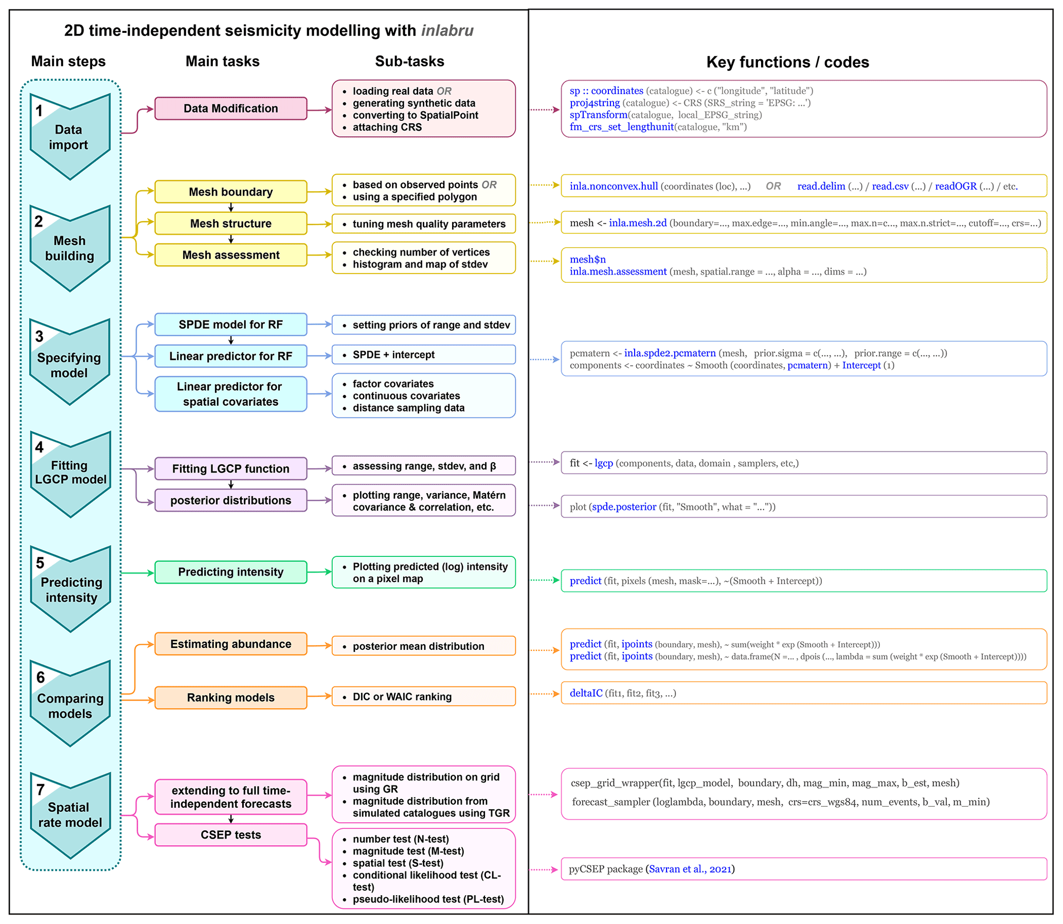
Figure 1 The workflow for generating spatial seismicity models in inlabru, with functions shown on the right.

In Bayliss et al. (2020) a range of California spatial forecast models were tested on how well the spatial model created by inlabru fitted the observed point locations, so were essentially a retrospective test of the spatial model alone in order to understand which components were most useful in developing and improving such models. Here we extend these models to full time-independent forecasts and test them in pseudo-prospective mode for California, again using the approach of testing different combinations of data sets as input data. We develop a series of new spatial models to compare with the smoothed seismicity forecast of Helmstetter et al. (2007). These models contain a combination of four different covariates that were found to perform well in terms of DIC in Bayliss et al. (2020). These are shown in Fig. 2 and include the strain rate (Kreemer et al., 2014) (SR) map, NeoKinema model slip rates (NK) attached to mapped faults in the UCERF3 model (Field et al., 2014), a past seismicity model (MS) and a fault distance map (FD) constructed using the UCERF3 fault geometry, with fault polygons buffered by their recorded dip. The past seismicity model used here is derived from events in the UCERF3 catalogue that occurred prior to 1984. For this data set, we fitted a model which contained only a Gaussian random field to the observed events, thus modelling the seismicity with a random field where we do not have to specify a smoothing kernel, the smoothing is an emergent property of the latent random field. This results in a smoothed seismicity map of events which occurred before our training dataset. This smoothed seismicity model also includes smaller magnitude events and those where the location or magnitude of the event is likely to be uncertain, so may account for some activity that is not observed or explicitly modelled (e.g. due to short-term clustering) at this time. Each of these components (SR, MS, NK, FD) is included as a continuous spatial covariate combined with a random field and intercept component. The M4.95+ events from 1985–2005 are used to construct the point process itself (M is used throughout to represent different magnitude scales depending on the source). The exact combination of components in a model is reflected in the model name as set out in Table 1: Model SRMS includes strain rate and past seismicity as spatial covariates, model FDSRMS includes fault distance, strain rate and past seismicity and model SRMSNK includes the strain rate, past seismicity and fault slip rates. More details on each of these model components and their performance in describing locations of observed seismicity can be found in Bayliss et al. (2020). Step 7 of the workflow covers the steps described below and results presented here.

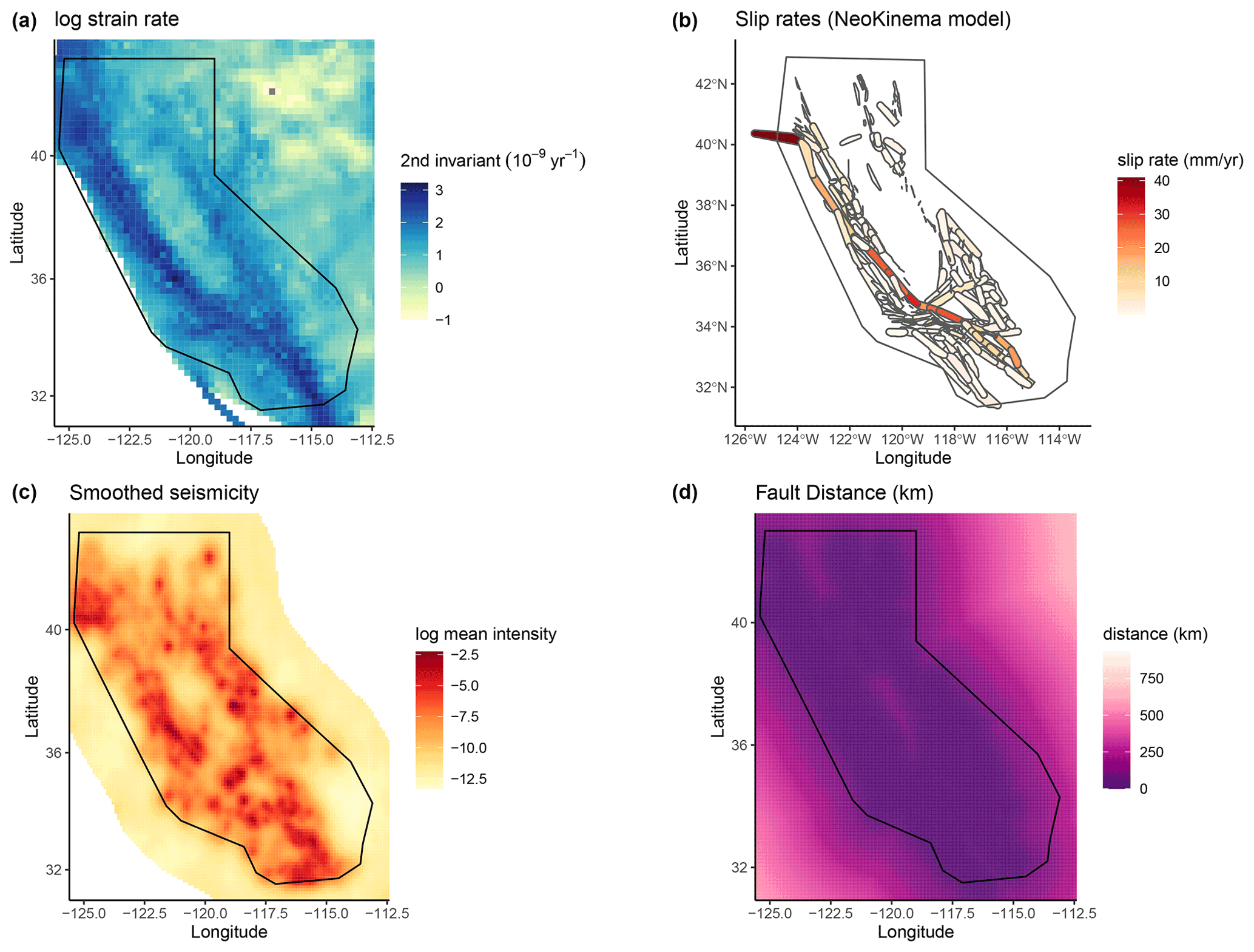
Figure 2 Input model covariates:  (a–d) strain rate (SR), NeoKinema slip rates from UCERF3 (NK), smoothed seismicity from a Gaussian random field for events before 1984 (MS), distance to nearest (UCERF3, dip and uniformly buffered) fault in km (FD).

2.1 Developing full forecasts from spatial models

The inlabru models provide spatial intensity estimates which can be converted to spatial event rates by considering the time scales involved. Since the models we develop here are to be considered time-independent, we assume that the number of events expected in this time period is “scaleable” in a straightforward manner, consistent with a (temporally homogeneous) spatially varying Poisson process. However we know that the rate of observed events is not Poissonian due to observed spatiotemporal clustering (Vere-Jones and Davies, 1966; Gardner and Knopoff, 1974) and that short time scale spatial clustering can lead to higher rates anticipated in areas where large clusters have previously been recorded (Marzocchi et al., 2014). To test the impact of clustering on our forecasts, we include models made from both the full and declustered catalogues, assuming that the full catalogues might overestimate the spatial intensity due to observed spatiotemporal clustering and forecast higher rates in areas with recent spatial clustering. We decluster the catalogue by removing events allocated as aftershocks or foreshocks within the UCERF3 catalogue, which were determined by a (Gardner and Knopoff, 1974) clustering algorithm (UCERF3 Appendix K). This results in 6 spatial models that we use from this point on, containing components as outlined in Table 1. Figures 3 and 4 respectively show the differences between the different models for the full and declustered catalogue models, with the posterior median of the log intensity for each of these on the diagonal. The top right part of each plot shows a pairwise comparison of the log median intensity of each model, while the bottom left component shows the pairwise differences in model variance. The differences in models are much clearer in the declustered catalogue models, once the clustering has been removed. This further highlights the role of random field in the full catalogue models is largely to account for spatial clustering. The model outcomes are constructed using an equal area projection of California and converted to latitude and longitude only in the final step before testing. This figure represents the set of models formed by the training data set.

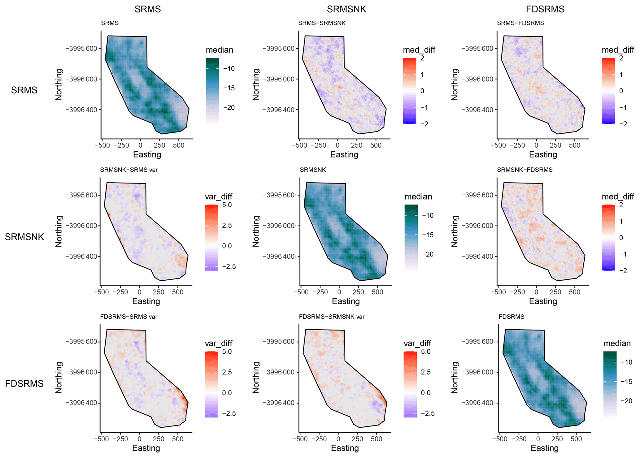
Figure 3 Pairwise comparison of models for full catalogue models. The top-right side of the plot shows differences in log median intensity and the lower left section shows the differences in model variances between the different models. The median log intensities for each model are shown on the diagonal. Models include combinations of smoothed past seismicity (MS), strain rate (SR), fault distance (FD) and fault slip rates (NK).

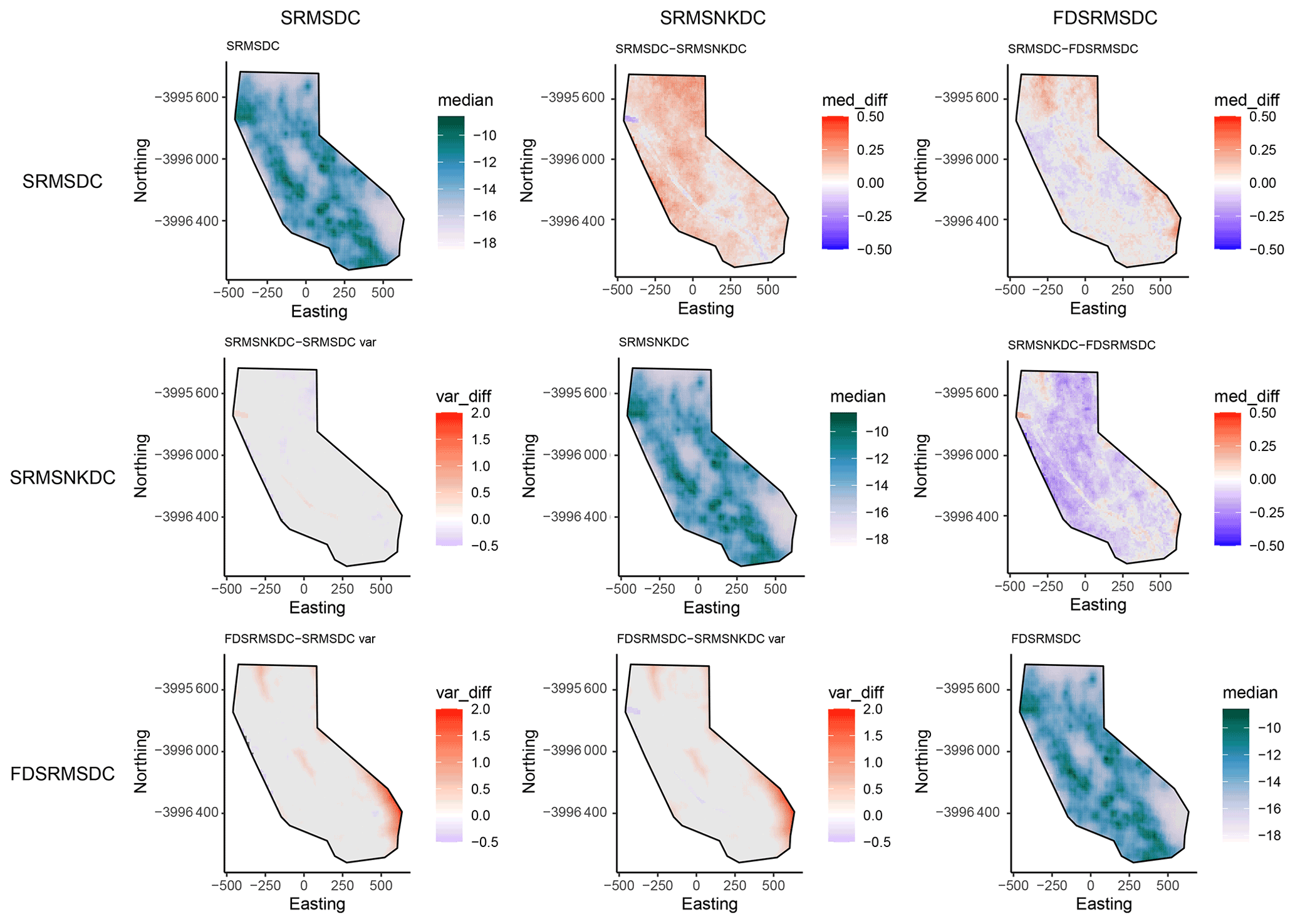
Figure 4 Pairwise comparison of models for declustered catalogue models. The top-right side of the plot shows differences in log median intensity and the lower left section shows the differences in model variances between the different models. The median log intensities for each model are shown on the diagonal. Models include combinations of smoothed past seismicity (MS), strain rate (SR), fault distance (FD) and fault slip rates (NK).

To extend this approach to a full forecast, we distribute magnitudes across the number of expected events according to a frequency-magnitude distribution. Given the small number of large events in the input training catalogue, a preference between a tapered Gutenberg-Richter (TGR) or standard Gutenberg-Richter magnitude distribution with a rate parameter a, related to the intensity λ, and an exponent b cannot be fully expressed. The choice of a b-value is not straightforward, as the b-value can be biased by several factors (Marzocchi et al., 2020) and is known to be affected by declustering (Mizrahi et al., 2021). In this case, we assume b=1 for both clustered and declustered catalogues, which is different from the maximum likelihood b-value obtained from the training catalogues (0.91 and 0.75 for the full and declustered catalogues, respectively). This was a pragmatic choice given that the high magnitude cut-off and therefore limited catalogue size is likely to result in a biased b-value estimate (Geffers et al., 2022). For the TGR magnitude distribution we assume a corner magnitude of M_c=8 for the California region as proposed by (Bird and Liu, 2007) and used in the Helmstetter et al. (2007) models.

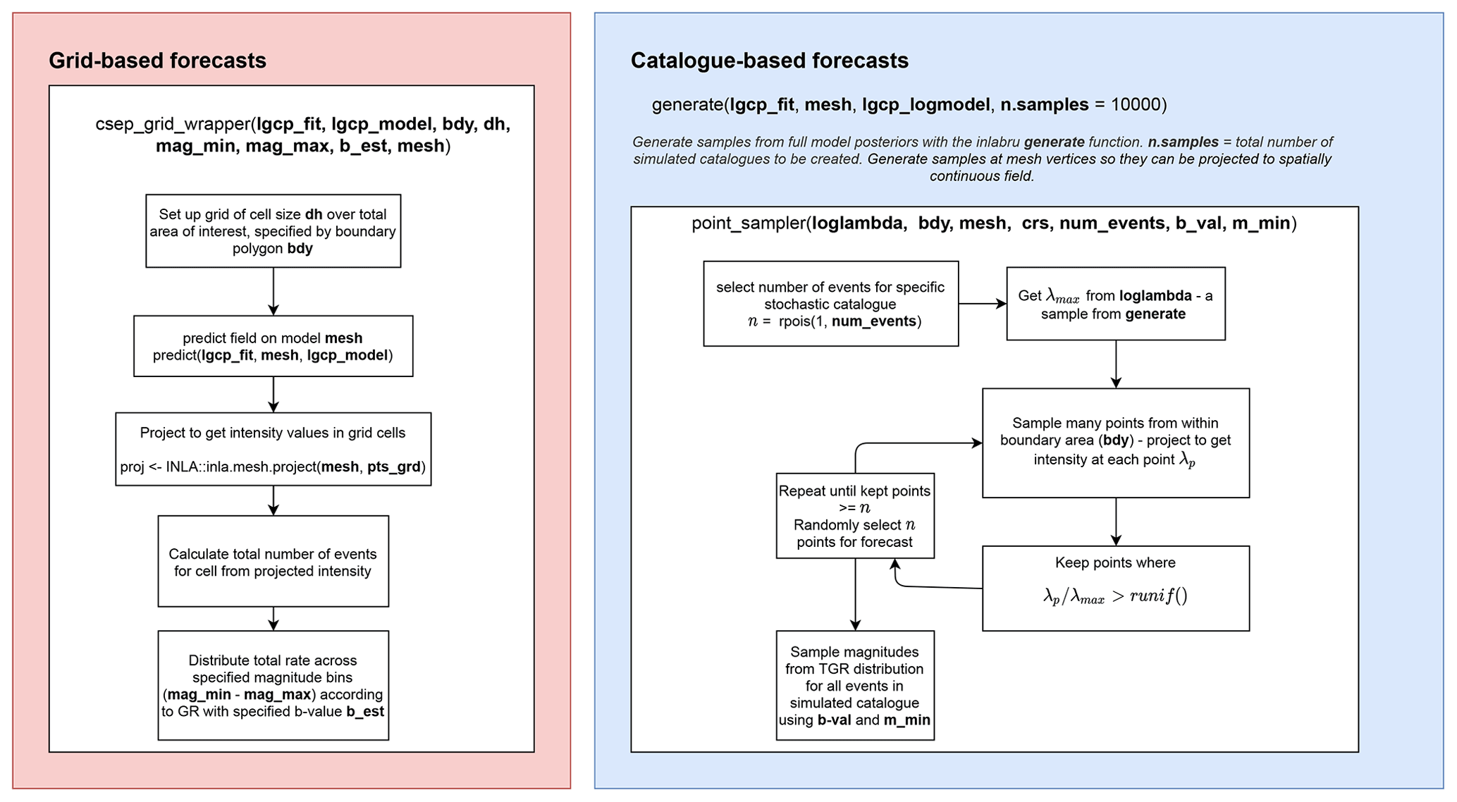
Figure 5 Schematic of the code for constructing grid-based (left) and simulated catalogue-based (right) earthquake forecasts given an inlabru LGCP intensity model. These represent step 7 of the workflow.

A schematic diagram showing how grid-based and catalogue-based approaches are applied is shown in Fig. 5, again to allow reproducibility of our results. The flowchart describes the necessary steps for extending a spatial model on a non-uniform grid to the specific formats required in forecast testing. For the gridded forecasts (which assume a uniform event rate or intensity within the area of each square element), we use the posterior median intensity as shown on the diagonals in Figs. 3 and 4, transformed to a uniform grid of 0.1 ° × 0.1° latitude and longitude within the RELM region. We use latitude-longitude here as preferred by the pyCSEP tests. Magnitudes are then distributed across magnitude bins on a cell-by-cell basis according to the chosen magnitude-frequency distribution and the total rate expected in the cell. In this paper, we show GR magnitudes for the gridded forecasts. For the catalogue-based forecasts, we generate 10 000 samples from the full posteriors of the model components to establish 10 000 realizations of the model spatial intensity within the testing polygon. We then sample a number of points consistent with the modelled intensity. In this case, we use the expected number of points given the mean intensity (as in step 6 in Fig. 1) for 1 year, and randomly select an exact number of events for a simulated catalogue from a Poisson distribution about the mean rate, scaled to the number of years in the forecast. To sample events in a way that is consistent with modelled spatial rates, we sample many points and calculate the intensity value at the sampled points given the realization of the model. We then implement a rejection sampler to retain points that have a significantly large intensity ratio compared to the largest intensity in the specific model realization, with points retained only if the intensity ratio is greater than a uniform random variable between 0 and 1, i.e. points are retained with a probability equal to $\mathrm{1}-\frac{{\mathit{\lambda }}_{\mathrm{p}}}{{\mathit{\lambda }}_{\max }}$. The set of retained points for each catalogue is then assigned a magnitude sampled from a TGR distribution, by methods described in Vere-Jones et al. (2001). Here, we only sample magnitudes from a TGR distribution in line with the approach of Helmstetter et al. (2007), to allow a like for like comparison with this benchmark.

2.2 CSEP tests

To test how well each forecast performs, we first test the consistency of the model forecasts, developed from data between 1985 and 2005, with observations from 3 subsequent and contiguous 5-year time periods, using standard CSEP tests for the number, spatial and magnitude distribution and conditional likelihood of each forecast. The original CSEP tests calculate a quantile score for the number (N), likelihood (L) (Schorlemmer et al., 2007) and spatial (S) and magnitude (M) (Zechar et al., 2010) tests, based on simulations that account for uncertainty in the forecast and a comparison of the observed and simulated likelihoods. We use 100 000 simulations of the forecasts to ensure convergence of the test results. The number test is the most straightforward, summing the rates over all forecast bins and comparing this with the total number of observed events. The quantile score is then the probability of observing at least N_obs events given the forecast, assuming a Poisson distribution of the number of events. Zechar et al. (2010) suggest using a modified version of the original N-test that tests the probability of (a) at least N_obs events with score δ₁ and (b) at most N_obs events with score δ₂ in order to test the range of events allowed by a forecast. Here we report both N-test quantile scores in line with this suggestion.

The likelihood test compares the performance of individual cells within the forecast. The likelihood of the observation given the model is described by a Poisson likelihood function in each cell and the total joint likelihood described by the product over all bins. The quantile score measures if the joint log-likelihood over many simulations falls within the tail of the observed likelihoods, with the score defined by the fraction of simulated joint log-likelihoods less than or equal to the observed. The conditional likelihood or CL test is a modification of the L test developed due to the dependence of L test results on the number of events in a forecast (Werner et al., 2010, 2011). The CL test normalizes the number of events in the simulation stage to the observed number of events in order to limit the effect of a significant mismatch in event number between forecast and observation. The magnitude and spatial tests compare the observed magnitude and spatial distributions by isolating these from the full likelihood. This is again achieved with a simulation approach and by summing and normalizing over the other components. For the M test, the sum is over the spatial bins while the S test sums over all magnitude bins to isolate the respective components of interest. The final test statistic in both cases is again the fraction of observed log likelihoods within the range of the simulated log likelihood values. In all cases small values are considered inconsistent with the observations. We use a significance value of 0.05 for the likelihood-based tests and 0.025 for the number tests to be consistent with previous forecast testing experiments (Zechar et al., 2013).

In the new CSEP tests (Savran et al., 2020) the test distribution is determined from the simulated catalogues rather than a parametric likelihood function. For the N test the construction of the test distribution is straightforward, being created from the number of events in each simulated catalogue and the quantile score calculated relative to this distribution. For the equivalent to the likelihood test a numerical, grid-based approximation to a point process likelihood is calculated (Savran et al., 2020). This is a more general approach than using the Poisson likelihood as in the grid-based tests, which penalizes models that do not conform to a Poisson model. The distribution of pseudo-likelihood is then the collection of calculated pseudo-likelihood results for each simulated catalogue. The spatial and magnitude test distributions are derived from the pseudo-likelihood in a similar fashion to the grid-based approach, as explained in detail by Savran et al. (2020). The quantile scores are calculated similar to the original test cases, but because the simulations are based on the constructed pseudo-likelihood rather than a Poisson likelihood, the simulated catalogue approach allows for forecasts which are overdispersed relative to a Poisson distribution. Similarly to the original tests, very small values will be considered inconsistent with the observations.

3 Full and declustered catalogue models

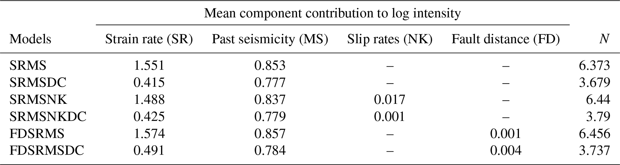
In constructing the three models both with and without clustering, we can examine relative contributions of the model components given differences in spatial intensity resulting from short-term spatiotemporal clustering. Table 1 shows the posterior mean component of the log intensity for each model both with and without clustering for M4.95+ seismicity, and the number of expected events per year for each model. The greatest contribution in the full catalogue models comes from the strain rate (SR) for each model, with the past seismicity also making a significant contribution to the intensity. For the models where the catalogue has been declustered, the contribution to the posterior mean from the past seismicity is only slightly lower while the SR contribution is much smaller, effectively swapping the relative contributions of these components. This suggests that the SR component is more useful when considering the full earthquake catalogue than when the catalogue has been declustered. In both full and declustered catalogue models, the number of expected events is similar across all three models, thus we expect the models to perform similarly in the CSEP N tests.

Figure 4 shows that the declustered catalogue models appear much smoother than those constructed from the full catalogue, as they have lower intensity in areas with large seismic sequences in the training period. They also have a smaller range in intensity than the full catalogue models, with the (median) highest rates lower and the (median) lowest rates higher than the full catalogue models, meaning they cover less of the extremes at either end.

Table 1 Posterior means of model components and number of expected events for full and declustered (DC) models.

4 Model testing

We now test the models using the pyCSEP package for python (Savran et al., 2021, 2022). We begin with the standard (grid-based) CSEP test models described by Schorlemmer et al. (2007) and Zechar et al. (2010) included in pyCSEP and described in Sect. 2.2.

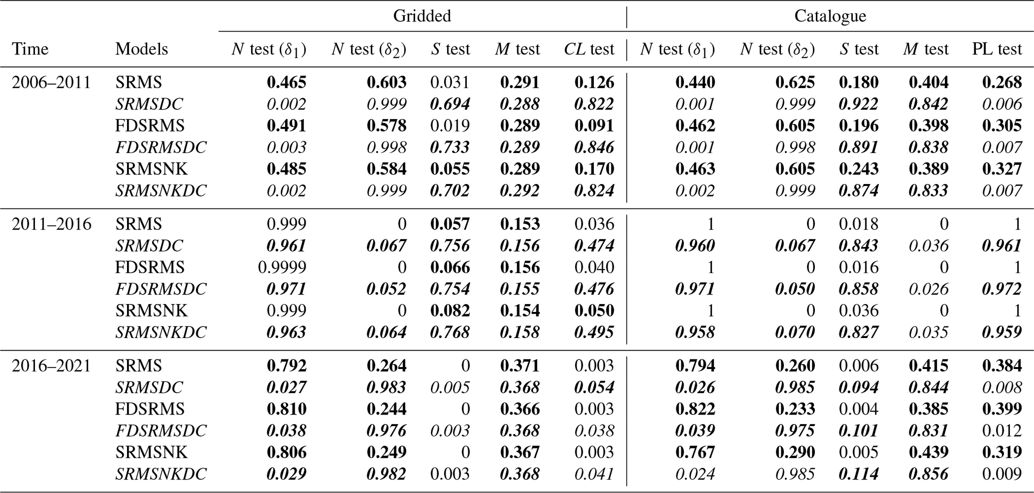
Table 2 Quantile scores for CSEP tests. Upper bounds for S, L and PL tests, lower bound for N. Bold indicates consistency with observations and italics highlight declustered models.

4.1 Grid-based forecast tests

We first compare the performance of our 5-year forecasts, developed with a training window of 1985–2005, over the testing period 1 January 2006–1 January 2011 with the Helmstetter et al. (2007) forecast. This testing time period was chosen to be consistent with the original RELM testing period. In this time, the comcat catalogue (https://earthquake.usgs.gov/data/comcat/, last access: 28 August 2022) includes 32 M4.95+ events in the study region defined by the RELM polygon. All the models, regardless of their components or which catalogue is used, perform well in the magnitude tests due to the use of the GR distribution. This is true even though we have used a fixed b-value of 1 for both catalogues, suggesting that the choice of b-value is not hugely influential in this testing period. The forecast tests are shown visually in Fig. 6 and the quantile scores are reported in Table 2 for all tests and time periods. A model is considered to pass a test if the quantile score is ≥0.05 for all tests except the N test, where the significance level is set at ≥0.025 for both score components and the model fails if either score fails (Schorlemmer et al., 2010; Zechar et al., 2010). In Fig. 6 the observed likelihood is shown as a coloured symbol (red circle for a failed test and green square for a passed test) and the forecast range is shown as a horizontal bar, for ease of comparison. In the number test (N test), the declustered forecasts significantly underpredict the number of expected events in all cases due to the much smaller number of expected events per year and the large number of events that actually occurred in the testing time period. In spatial testing (S test), the full catalogue models all perform poorly. In contrast, the declustered catalogue models all pass the S test. In the conditional likelihood tests (CL test), all of the models perform well and pass the CL test (Fig. 6), with the declustered models performing better due to better spatial performance.

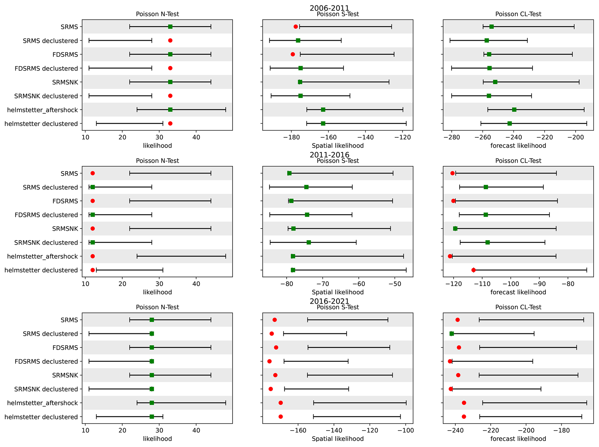
Figure 6 Grid-based forecast tests for all forecasts for three 5-year time periods: 2006–2011 (top), 2011–2016 (middle) and 2016–2021(bottom). The bars represent the 95 % confidence interval derived from simulated likelihoods from the forecast, while the symbol represents the observed likelihood for observed events. The green square identifies that a model has passed the test and a red circle indicates inconsistency between forecast and observation. The forecasts are compared to both the full (Helmstetter aftershock) and declustered models of Helmstetter et al. (2007). Models include combinations of smoothed past seismicity (MS), strain rate (SR), fault distance (FD) and fault slip rates (NK).

We then repeat the tests for two additional 5-year periods of California earthquakes illustrated in Fig. 6. In all time windows, the M test results remain consistent across all models. In the 2011–2016 period, there are 13 M4.95+ events within the RELM polygon, and this significant reduction in event number means that our full catalogue models and the Helmstetter models all significantly overestimate the actual number of events, with the true number outside of the 95 % confidence intervals of the models. In contrast, most of the models perform better in the S test during this time period with all full catalogue models and all declustered catalogue models recording a passing quantile score (Table 2). Each of the models made with a declustered catalogue passes the CL test, and the full catalogue model with slip rates also passes.

In the 2016–2021 period (Fig. 6 bottom) there are 30 M4.95+ events, which is within the confidence intervals shown for all tested models so all models pass the N test for the first time. However none of the tested models pass the S test due to the spatial distribution of the events in this time period being highly clustered in areas without exceptionally high rates, even for models developed from the full catalogue. The CL test results for the 2016–2021 period show that none of the models perform particularly well in this time period, with only one of the declustered catalogue models passing the test, and only barely.

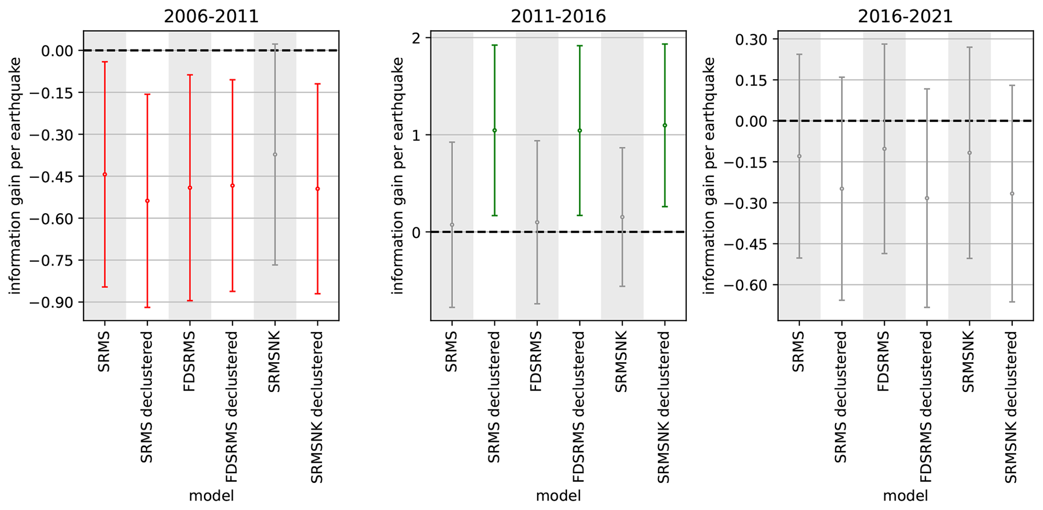
Figure 7 T-test results for the inlabru models showing information gain per earthquake relative to the full Helmstetter et al. (2007) model (Helmstetter aftershock in Fig. 6) for three time periods. Red indicates forecasts are worse in terms of information gain and green indicates forecasts performing better than the benchmark forecast. Grey forecasts are not significantly different in terms of information gain. Models include combinations of smoothed past seismicity (MS), strain rate (SR), fault distance (FD) and fault slip rates (NK).

These statistical tests (N, S, M and CL) investigate the consistency of a forecast made during the training window with the observed outcome. They do not compare the performance of models directly with each other, but with observed events. One method of comparing forecasts is by considering their information gain relative to a fixed model with a paired T-test (Rhoades et al., 2011). Here, we implement the paired T-test for the gridded forecast to test the performance against the Helmstetter et al. (2007) aftershock forecast as a benchmark, because it performed best in comparison to other RELM models in previous CSEP testing over various time scales (Strader et al., 2017). The results of the comparison are shown in Fig. 7. For the first time period (2006–2011) the models perform similarly in terms of information gain, and all of the inlabru models perform worse than the Helmstetter model. For the 2011–2016 period, the inlabru models developed from the declustered catalogues perform better in terms of information gain than those developed from the full catalogue and significantly better than the Helmstetter model. In the most recent testing period (2016–2021), the inlabru models have an information gain range that includes the Helmstetter model. Together these results imply that the inlabru models provide a positive and significant information gain on a 5–10-year time period after the end of the training period for declustered catalogue models, and not otherwise.

4.2 Simulated catalogue forecasts

Our second stage of testing uses simulated catalogues in order to make use of the newer CSEP tests (Savran et al., 2020). We use the number, spatial and pseudo-likelihood (PL) tests to evaluate these forecasts, with the PL test replacing the grid-based L test. In our case, as described above, the number of events in the simulated catalogues is inherently Poisson due to the way they are constructed, but the spatial distribution is perturbed from a homogeneous Poisson distribution due to the contributions of model covariates and the random field itself (e.g. see Eq. 1, where a homogenous Poisson process would include only the intercept term β₀) and the parameter values are sampled from the posterior at each simulation and therefore vary from simulation to simulation. Figure 8 shows the test distributions for each forecast as a letter-value plot (Hofmann et al., 2011), an extended boxplot which includes more quantiles of the distribution until the quantiles become too uncertain to discriminate. This allows us to understand more of the full distribution of model pseudo-likelihood than a standard quantile range or boxplot, while allowing easy comparisons between the results for different forecast models.

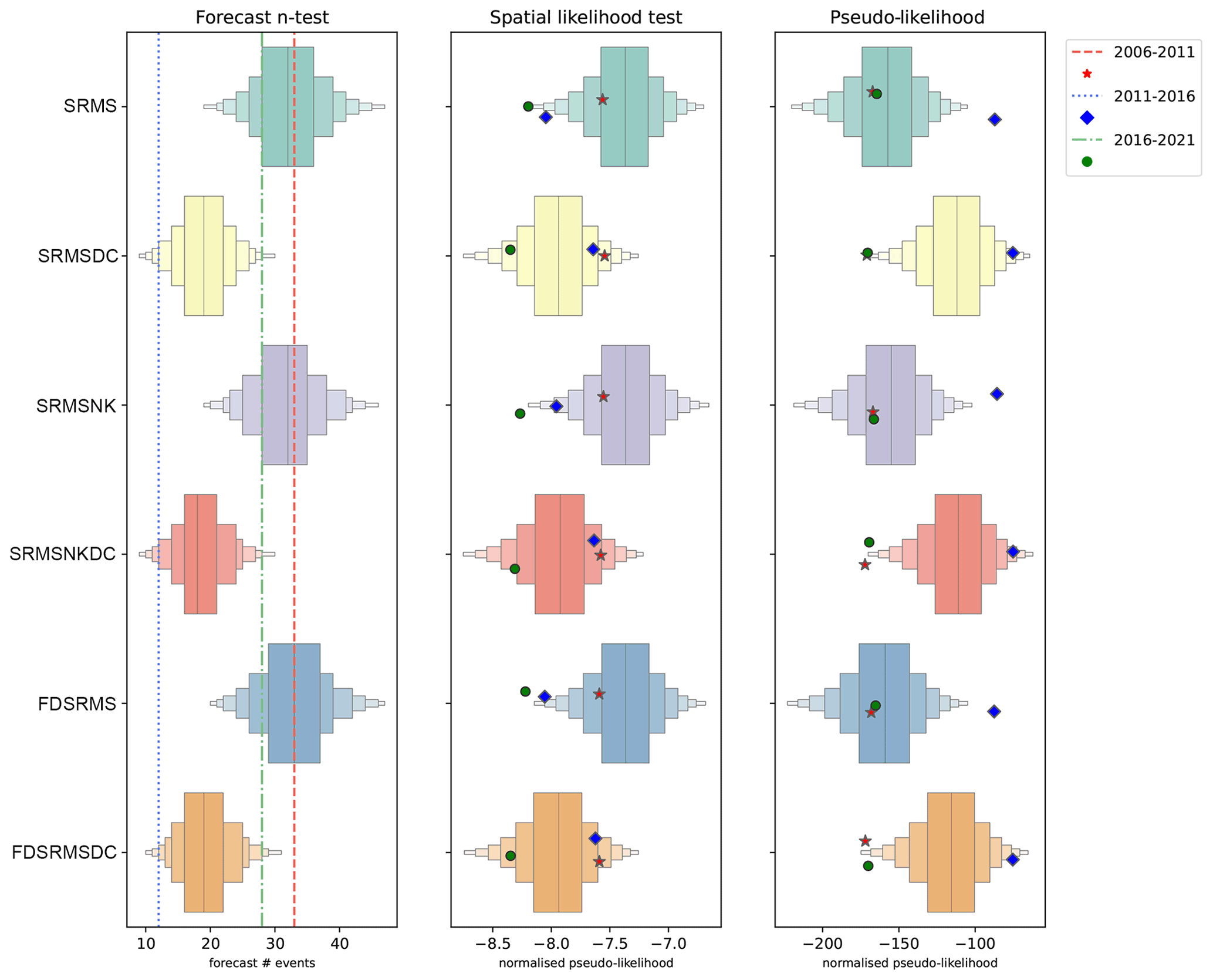
Figure 8 N test, S test and pseudo-likelihood results for each of the 6 inlabru models when forecasts are generated from 10 000 synthetic catalogues sampling from the full inlabru model posteriors. For the N test, the number of observed events for the 2006–2011, 2011–2016 and 2016–2021 are shown by the red, blue and green dashed lines, respectively. For the S and pseudo-likelihood tests, the observed test statistic for each time period is shown as a symbol (red star for 2006–2011, blue diamond for 2011–2016 and green circle for 2016–2021). Models include combinations of smoothed past seismicity (MS), strain rate (SR), fault distance (FD) and fault slip rates (NK), where DC indicates a model built with a declustered catalogue.

We expect the grid-based and simulated catalogue approaches to have similar results in terms of the magnitude (M) tests due to the similarity of magnitude distributions used in construction. All models pass the M test in the testing periods 2006–2011 and 2016–2021, but only the declustered models pass the M test in the 2011–2016 testing period when the number of observed events was smaller. Similarly, we do not expect significant differences in the N-tests with this approach, since our method of determining the number of events will result in a Poisson distribution of the number of events. However, since the number of events varies in each synthetic catalogue we can look at the distribution of the number of events in the synthetic data produced by the ensemble of forecast catalogues relative to the observed number. This is shown in the left panel of Fig. 8, with the observed number of events for each time period shown with a dashed line. Again, the declustered models do better in the 2011–2016 period, although it is clear that the observed number of events is low even for them.

We might expect the most noticeable differences to occur in the spatial test, because it measures the spatial component consistency with observed events and because we are now using the full posterior distribution of spatial components, and therefore potentially allowing more variation in the observed spatial models. The middle panel of Fig. 8 shows the spatial likelihood distribution constructed from simulated catalogues.

Similar to the grid-based examples, for the 2006–2011 period (red star indicator) the spatial performance of the SRMS and FDSRMS models is better when the full, rather than declustered catalogue, has been used in model construction.

All of the models pass the S test when considering quantile scores in this time period. Similarly, when testing the 2011–2016 period (test statistic shown with a blue diamond), all of the models built from the declustered catalogue pass the S test, while the full catalogue models do more poorly. In 2016–2021 (green circle), the spatial performance of all models is again poor. The best-performing models in this time period are the FDSRMS declustered and SRMSNK declustered models (Table 2), with the declustered catalogue models generally doing better than the full catalogue models.

Finally, the pseudo-likelihood test (Fig. 8, right) incorporates both spatial and rate components of the forecast, much like the grid-based likelihood. For the inlabru models, the preference between the models for the full and declustered catalogues changes with time period with both sets of models doing poorly in the 2016–2021 period (green circle). All of the full catalogue models pass in 2006–2011 and in 2016–2021. Like the grid-based likelihood test, the pseudo-likelihood test penalizes for the number of events in the forecast, which allows the full catalogue models to pass the pseudo-likelihood test even when they have poor spatial performance, as in the 2016–2021 testing period.

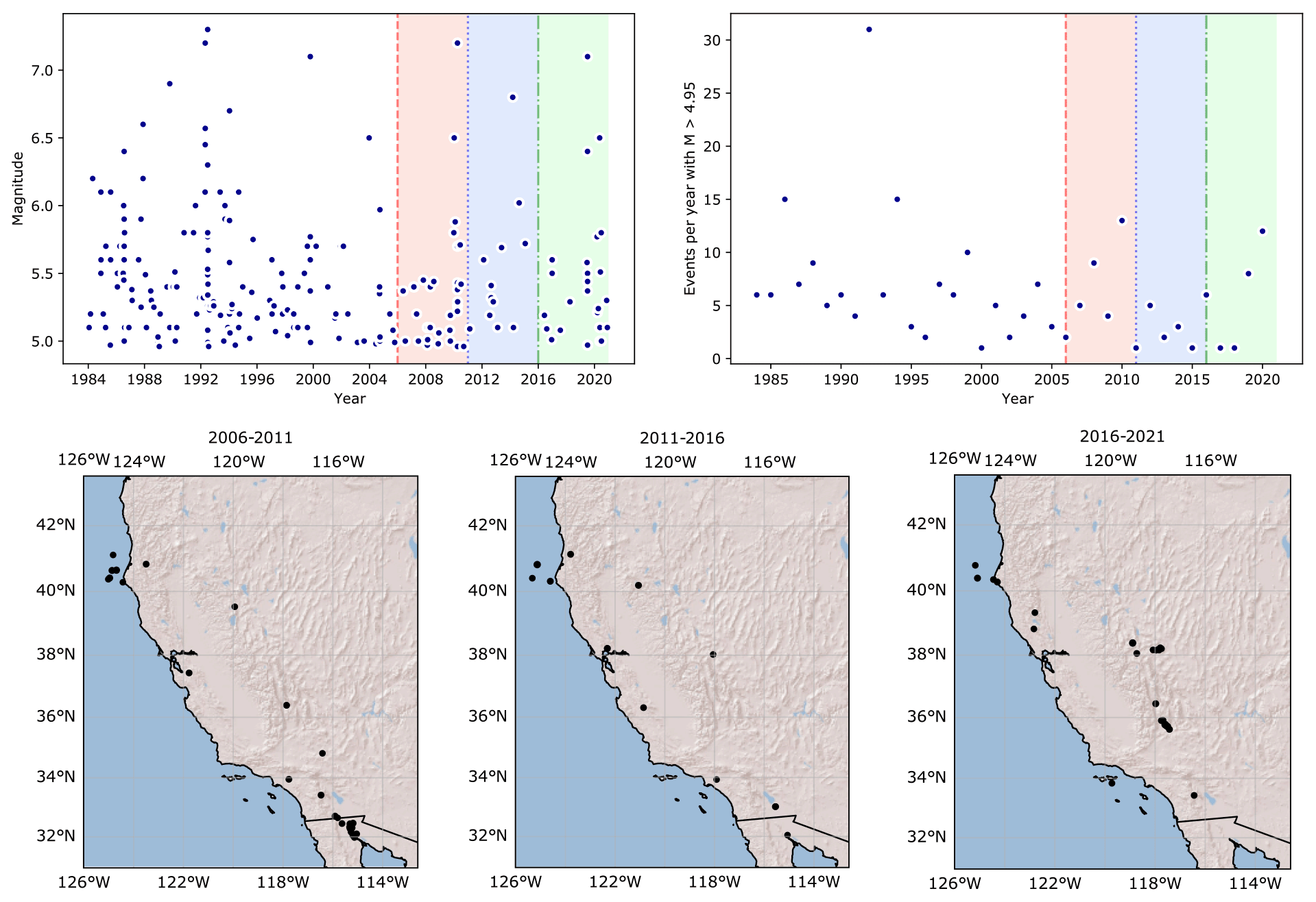
Figure 9 Top: Catalogue of events in California from 1985–2021. The period 1985–2005 is used for model construction, and the three testing periods are shown with red, blue and green backgrounds. The left panel shows the magnitude of events in time and the right the number of events in each year. Bottom: the comcat catalogues for the three 5-year testing intervals.

5 Discussion

5.1 Number of events

While the full catalogue models performed well in the tests for the first 5-year time window, the other two sets of test results were less promising. This can be largely explained by the number of events that occurred in the 10-year period from 2006–2016 (red and blue backgrounds in Fig. 9, top right). In this time 45 events were recorded in the comcat catalog, compared to 32 events in the 5 years between 2006–2011. In the 20 years from 1985–2005 used in our model construction, a total of 155 events with M > 4.95 were recorded, which is an average of 7.8 events per year. Bayona et al. (2022) found that 10-year prospective tests of hybrid RELM models mostly overestimated the number of events, again due to the small number of events in the 2011–2020 testing period used in their analysis. Helmstetter et al. (2007) explicitly used the average number of events per year with magnitude > 4.95 (7.38 events) to condition their models. It is therefore not surprising that the declustered forecasts perform oppositely, with poor performance in the 2006–2011 time period and better performances in the 2011–2016 time period when fewer events occurred. This is a common issue in CSEP testing, reported both in Italy when the 5-year tests occurred in a time period with a large cluster of events in a historically low seismicity area (Taroni et al., 2018) and in New Zealand, where the Canterbury earthquake sequence occurred in the middle of the CSEP testing period (Rhoades et al., 2018) resulting in significantly more events than expected. Strader et al. (2017) found that 4 of the original RELM forecasts overpredicted the number of events in the 2006–2011 time window and 11 overpredicted the number of events in the second 5-year testing window (2011–2016), including the Helmstetter model. Overall, the inlabru model N test results were comparable to the Helmstetter model performance in the grid-based assessment and performed well at forecasting at least the minimum number of events in all but the declustered models in the first testing period (Table 2).

5.2 Full and declustered catalogue models

We did not filter for main shocks in the observed events, so we might expect the N test results for the declustered models to do poorly, but they were consistent with observed behaviour in 2 of the 3 tested time periods in both the grid-based and catalogue-based testing. If we consider only the lower bound of the N test, the declustered models pass the test in the full 2011–2021 time period and only perform poorly in 2006–2011, a time period which arguably contained many more than the average number of events (Fig. 9). Similarly, the full catalogue models do poorly on the upper N test in 2011–2016 but otherwise pass in time windows with higher numbers of events.

The declustered models pass spatial tests more often than the full catalogue models because they are less affected by recent clustering, and perhaps benefit from being smoother overall than the full catalogue models (Figs. 3 and 4). The superior performance of the declustered models may not have been entirely obvious had we tested only the 2006–2011 period and relied solely on the “pass” criterion from the full suite of tests: only the full-catalogue (non-declustered) synthetic catalogue forecast models get a pass in all consistency tests in this time period. This highlights a need for forecasts to be assessed over different time scales in order to truly understand how well they perform, a point previously raised by Strader et al. (2017) when assessing the RELM forecasts, and more generally embedded in the evaluation of forecasting power since the early calculations of Lorenz (1963) for a simple but nonlinear model for the earth's atmosphere in meteorological forecasting.

We conclude that neither a full nor declustered catalogue necessarily gives a better estimate of the future number of events in any 5-year time period, although the declustered models tend to perform better spatially, and may be more suitable for longer term forecasting. Given that different declustering methods may retain different specific events and different total numbers of events, different declustering approaches may lead to significant differences in model performances, especially in time periods with a small number of events in the full catalogue. To truly discriminate between which approach is best, a much longer testing time frame would be needed to ensure a suitably large number of events.

5.3 Spatial performance of gridded and simulated catalogue forecasts

In general, the simulated catalogue-based forecasts were more likely to pass the tests than the gridded models. This is most obvious in the first testing period, when the simulated catalogue-based models based on the full catalogue passed all tests and those for the declustered catalogues only failed due to the smaller expected number of events. Similarly, in the most recent testing period (2016–2021) the simulated catalogue forecasts are able to just pass the S test where all models fail in the gridded approach. Bayona et al. (2022) suggested that the spatial performance of multiplicative hybrid models in the 2011–2020 period suffered due to the presence of significant clustering associated with the 2016 Hawthorne Swarm in northwestern Nevada at the edge of the testing region and the 2019 Ridgecrest sequence, and that the absence of large on-fault earthquakes in the testing period had potentially affected model performance of hybrids with geodetic components. They further suggested that the performance of these models in this testing period could be a result of reduced predictive ability with time, since hybrid models have performed better in retrospective analyses.

The simulated catalogue approach allows us to consider more aspects of the uncertainty in our model. For example, we could further improve upon this by considering potential variation in the b-value in the ensemble catalogues which arises from magnitude uncertainties, an issue that may be particularly relevant when dealing with homogenized earthquake catalogues (Griffin et al., 2020) or where the b-value of the catalogue is more uncertain (Herrmann and Marzocchi, 2020).

5.4 Roadmap – where next?

The main limitation of the work presented here, and many other forecast methodologies, is how aftershock events are handled. Our choice of (a relatively high) magnitude threshold for modelling may have also benefited the full model by ignoring many small magnitude events that would be removed by a formal declustering procedure. The real solution to this is to formally model the clustering process.

The approach presented here strongly conforms with current practice. In time-independent forecasting and PSHA, catalogues are routinely declustered to be consistent with Poisson occurrence assumptions. Operational forecasting already relies heavily on models, such as the epidemic type aftershock sequence model (ETAS, Ogata, 1988), to handle aftershock clustering (Marzocchi et al., 2014), but few attempts have been made to account for background spatial effects beyond a simple continuous Poisson rate. The exceptions to this are changes to the spatial components of ETAS models (Bach and Hainzl, 2012), the recent developments in spatially varying ETAS (Nandan et al., 2017) and extensions to the ETAS model that also incorporate spatial covariates (Adelfio and Chiodi, 2020). However, the more versatile inlabru approach allows for more complex spatial models than has yet been implemented with these approaches. The inlabru approach also provides a general framework to test the importance of different covariates in the model, and a fully Bayesian method for forecast generation as we have implemented here.

One way to handle these conflicts is to model the seismicity formally as a Hawkes process, where the uncertainty in the tradeoff between the background and clustered components is explicit and can be formally accounted for. In future work we will modify the workflow of Fig. 1 to test the hypothesis that this approach will improve the ability for inlabru to forecast using both time-independent and time-dependent models.

6 Conclusions

We have demonstrated the first extension of spatial inlabru intensity models for seismicity to fully time-independent models, created using both classical uniform grids and fully Bayesian catalogue-type forecasts that make use of full model posteriors. We demonstrate that the inlabru models perform well in pseudo-prospective testing mode, passing the standard CSEP tests and performing favourably in competition with existing time-independent CSEP models over the 2006–2011 period. Forecasts constructed using a declustered catalogue as input performed less well in terms of the number of expected events, but nevertheless described spatial seismicity well even where the testing catalogue had not been declustered, and the declustered models performed better than the full catalogue models in the 2011–2016 testing period. Further testing on longer time scales would be necessary to assess if full or declustered catalogues provide a better estimate of the number of expected events on the time scales examined here. In the most recent testing period, i.e. the one with the longest time lag between the learning and the testing phase, neither full or declustered catalogue models perform well, suggesting a possible degree of memory loss over a decadal time scale in both clustered and declustered seismicity. Simulated catalogue forecasts that make use of full model posteriors passed consistency tests more often than the grid-based equivalents, most likely due to their ability to account for uncertainty in the model itself, including test metrics that do not rely on the Poisson assumption. This demonstrates the potential of fully Bayesian earthquake forecasts that include spatial covariates to improve upon existing forecasting approaches.