the Creative Commons Attribution 4.0 License.
the Creative Commons Attribution 4.0 License.
 | 06 Oct 2022
Partitioning the contributions of dependent offshore forcing conditions in the probabilistic assessment of future coastal flooding
Deborah Idier
Remi Thieblemont
Goneri Le Cozannet
François Bachoc
Getting a deep insight into the role of coastal flooding drivers is of great interest for the planning of adaptation strategies for future climate conditions. Using global sensitivity analysis, we aim to measure the contributions of the offshore forcing conditions (wave–wind characteristics, still water level and sea level rise (SLR) projected up to 2200) to the occurrence of a flooding event at Gâvres town on the French Atlantic coast in a macrotidal environment. This procedure faces, however, two major difficulties, namely (1) the high computational time costs of the hydrodynamic numerical simulations and (2) the statistical dependence between the forcing conditions. By applying a Monte Carlo-based approach combined with multivariate extreme value analysis, our study proposes a procedure to overcome both difficulties by calculating sensitivity measures dedicated to dependent input variables (named Shapley effects) using Gaussian process (GP) metamodels. On this basis, our results show the increasing influence of SLR over time and a small-to-moderate contribution of wave–wind characteristics or even negligible importance in the very long term (beyond 2100). These results were discussed in relation to our modelling choices, in particular the climate change scenario, as well as the uncertainties of the estimation procedure (Monte Carlo sampling and GP error).
- Article
(4544 KB) - Full-text XML
-
Supplement
(1624 KB) - BibTeX
- EndNote


Coastal flooding is generally not caused by a unique physical driver but by a combination of them, including mean sea level changes, atmospheric storm surges, tides, waves, river discharges, etc. (e.g. Chaumillon et al., 2017). The intensity of surge itself depends on atmospheric pressure and winds as well as on the site-specific shape of shorelines and water depths (bathymetry). Hence, compound events, resulting from the co-occurrence of two or more extreme values of these processes is a significant reason for concern regarding adaptation. For example, flood severity is significantly increased by the co-occurrence of extreme waves and surges at a number of major tide gauge locations (Marcos et al., 2019), of high sea level and high river discharge in the majority of deltas and estuaries (Ward et al., 2018), and of high sea level and rainfall at major US cities (Wahl et al., 2015). This intensification of compound flooding is expected to be exacerbated under climate change (Bevacqua et al., 2020). A deeper knowledge of coastal flooding drivers is thus a key element for the planning of adaptation strategies such as engineering, sediment-based or ecosystem-based protection, accommodation, planned retreat, or avoidance (Oppenheimer et al., 2019; see also the discussion by Wahl et al., 2017).
In this study, we analyse compound coastal flooding at the town of Gâvres on the French Atlantic coast. This site has been impacted by four major coastal flooding events since 1905 (Idier et al., 2020a), in particular, by the storm event Johanna on 10 March 2008, which resulted in about 120 flooded houses (Gâvres mayor: personal communication, 2019; Idier et al., 2020a). Flooding processes at this site are known to be complex (macrotidal regime and wave overtopping, variety of natural and human coastal defences, various exposure to waves due to the complex shape of shorelines; see a thorough investigation by Idier et al., 2020a). We aim to unravel which offshore forcing conditions among wave characteristics (significant wave height, peak period, peak direction), wind characteristics (wind speed at 10 m, wind direction) and still water level (combination of mean sea level, tides and atmospheric surges) drive severe compound flood events, considering projected sea level rise (SLR), up to 2200.
We adopt here a probabilistic approach to assess flood hazard; i.e. we aim to compute the probability of flooding and to quantify the contributions of the drivers with respect to the occurrence of the flooding event by means of global sensitivity analysis, denoted GSA (Saltelli et al., 2008). This method presents the advantage of exploring the sensitivity in a global manner by covering all plausible scenarios for the inputs' values and by fully accounting for possible interactions between them. The method has been applied successfully in different application cases in the context of climate change (e.g. Anderson et al., 2014; Wong and Keller, 2017; Le Cozannet et al., 2015, 2019a; Athanasiou et al., 2020).
Unlike these previous studies, the application of GSA to our study site faces two main difficulties: (1) the physical processes related to flooding are modelled with numerical simulations that have an expensive computational time cost (i.e. larger than the simulated time), which hampers the Monte Carlo-based procedure for estimating the sensitivity measures, and (2) the offshore forcing conditions cannot be considered independent, and the probabilistic assessment should necessarily account for their statistical dependence. This complicates the decomposition of the respective contributions of each physical drivers in GSA (see a discussion by Do and Razavi, 2020).
Our study proposes a procedure to overcome both difficulties by combining multivariate extreme value analysis (Heffernan and Tawn, 2004; Coles, 2001) with advanced GSA techniques specifically adapted to handle dependent inputs (Iooss and Prieur, 2019) and probabilistic assessments (Idrissi et al., 2021). To overcome the computational burden of the procedure, we adopt a metamodelling approach; i.e. we perform a statistical analysis of existing databases of pre-calculated high-fidelity simulations to construct a costless-to-evaluate statistical predictive model (named “metamodel” or “surrogate”) to replace the long-running hydrodynamic simulator (see e.g. Rohmer et al., 2020).
The article is organized as follows. Section 2 describes the test case of Gâvres, the data and the numerical hydrodynamic simulator used to assess flood hazard. In Sect. 3, we describe the overall procedure to partition the uncertainty contributions of dependent offshore forcing conditions for future coastal flooding. The procedure is then applied to Gâvres, and results are analysed in Sect. 4 for future climate conditions. In Sect. 5, the influence of different scenario assumptions in addition to the offshore forcing conditions is further discussed, namely the magnitude of the flooding events, the influence of the climate change scenario, the digital elevation model (DEM) used as input of the hydrodynamic numerical model and the intrinsic stochastic character of the waves.
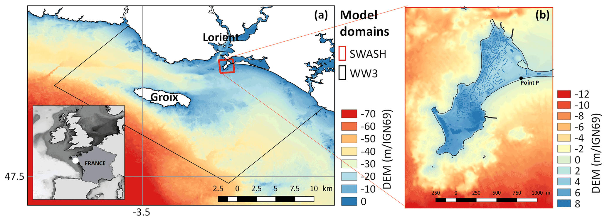
Figure 1Digital elevation model (DEM expressed with respect to IGN69, French national vertical datum) and computational domain of the study site of Gâvres for the spectral wave model WW3 (a) and for the non-hydrostatic phase-resolving model SWASH (b). The insert in (a) provides the regional setting. The point P indicates an observation point on the coast. Adapted from Idier et al. (2020a).
2.1 Numerical modelling of flooding
The considered case study corresponds to the coastal town of Gâvres on the French Atlantic coast in a macrotidal environment (mean spring tidal range: 4.2 m). Since 1864, more than 10 coastal flooding events have hit Gâvres (Le Cornec et al., 2012). The flooding modelling is based on the non-hydrostatic phase-resolving model SWASH (Zijlema et al., 2011), which allows for simulating wave overtopping and overflow. The implementation and validation on the study site is described in Idier et al. (2020a), and we summarize here the main aspects. The computational domain and the digital elevation model (DEM) are shown in Fig. 1 (red domain). The DEM (denoted DEM 2015) is representative of the 2015 local bathymetry and topography and of the 2018 coastal defences. The space and time resolution are, respectively, 3 m in the horizontal dimension, two layers along the vertical dimension and more than 10 Hz. The offshore wave conditions (south of the island of Groix) are propagated to the boundaries of the SWASH model using the spectral wave model WW3 (WAVEWATCH III; Ardhuin et al., 2010), taking into account the local tide, atmospheric surge and wind (see large spatial domain in Fig. 1a). The combined WW3–SWASH model chain has been validated with respect to the area that was flooded during the Johanna storm event (which occurred on 10 March 2008): the model slightly overestimates the number of flooded houses by about 3 %, which can be considered very satisfactory for such complex environments.
The inland impact of a storm event is assessed by estimating the total water volume Y that has entered the territory at high tide. This is performed by first running the WW3 model (over 2 h to reach steady wave conditions) and then the SWASH model by considering a time span of 20 min (with 5 min spin-up) and steady-state offshore forcing conditions. The value of Y is the volume at the end of the simulation. Such simulation costs about 90 min of time computation on approximately 48 cores. Figure 2 provides the maps of water depth and the corresponding value of Y computed with the above-described simulator for five different storm events. In the study, we use the volume value Y = 50, 2000 and 15 000 m3 to categorize the flooding event as “minor”, “moderate” and “very large”. In addition, to account for the random character of waves, the modelling of the coastal flood induced by overtopping processes is combined with a random generation of wave characteristics in SWASH as described by Idier et al. (2020b). For given offshore forcing conditions, the simulation is repeated nr = 20 times, and the median value (denoted mY) of Y is calculated. The impact of wave stochasticity is further discussed in Sect. 5.1.
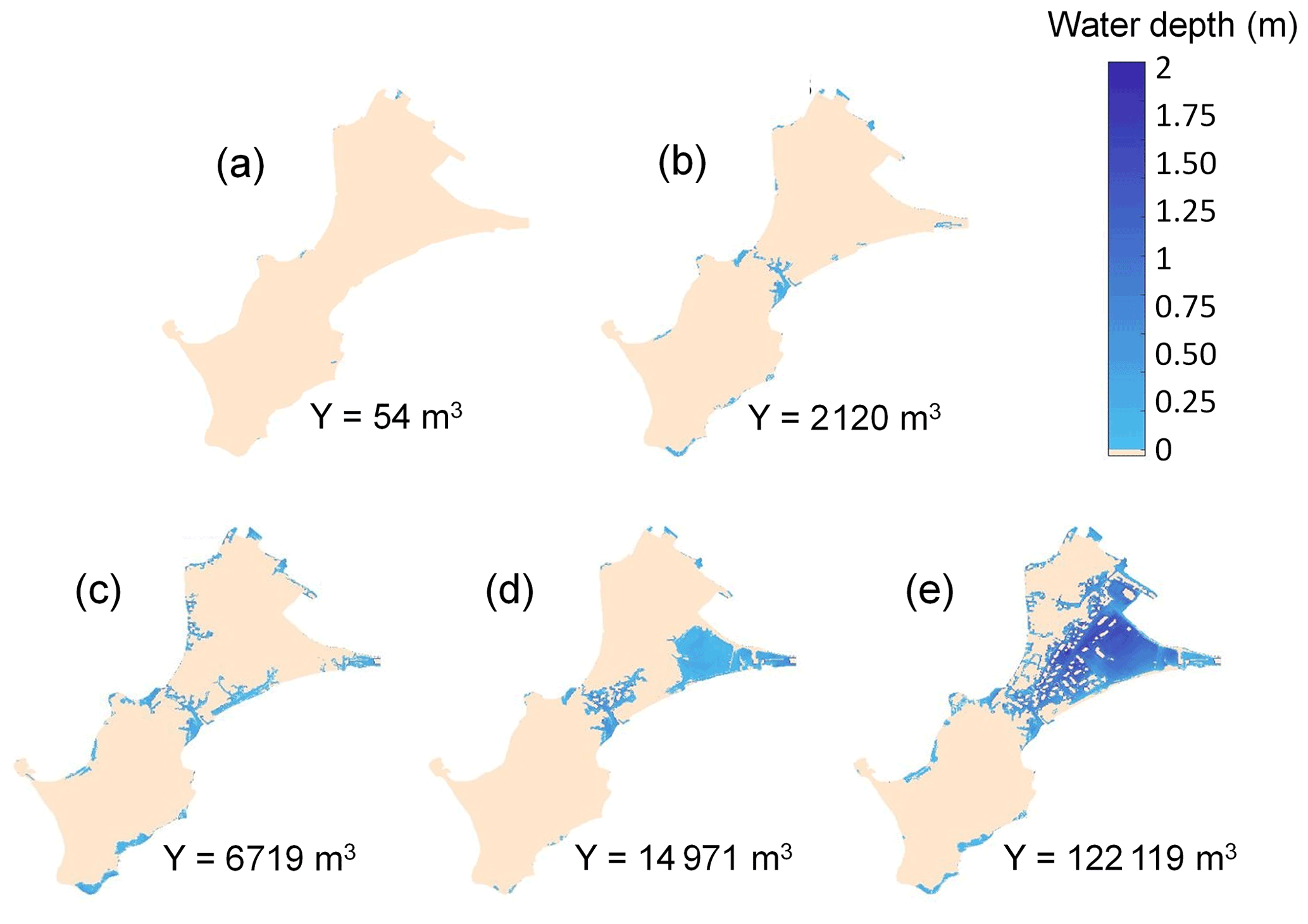
Figure 2Examples of five maps of water depth modelled by the numerical simulator described in Sect. 2 using DEM 2015. The value of the flood-induced inland water volume Y is indicated for the five cases. In the study, the volume values of 50, 2000 and 15 000 m3 have been selected to categorize the flooding event as minor, moderate and very large. Note that due to lack of numerical results with Y close to 15 000 m3 in the database of simulation results (see Sect. 5), panel (d) is provided using DEM 2008 instead.

Figure 3Overview of the N = 50 000 randomly generated samples of offshore conditions (red dots). Blue dots correspond to the hindcast conditions used to fit the statistical methods described in Sect. 3.3. Green dots and squares correspond to the n = 144 training data points used to set up the GP metamodel (the selection approach is detailed in Sect. 3.2). The squares correspond to cases that are deliberately selected outside the range of the red dots to cover a broader range of situations. SWL is defined with respect to the mean sea level (MSL).
2.2 Offshore forcing conditions
The modelling chain is forced by six offshore conditions, namely the still water level (SWL) – expressed with respect to the mean sea level, the significant wave height (Hs), the peak period (Tp), the direction (Dp), the wind speed at 10 m (U) and wind direction (Du). These are defined using a database composed of hindcasts of past conditions offshore of the study site over the period 1900–2016. This dataset was built via the concatenation of hindcasts of different sources (see Table 1 of Idier et al., 2020a, for further details) completed by bias corrections using a quantile–quantile correction method. A total of > 80 000 past events characterized by (SWL, Hs, U, Tp, Dp and Du) taken at the time instant of the high tide are used in the following to constrain the statistical methods of Sect. 3. The visual analysis of the extracted conditions (blue dots in Fig. 3) suggests a moderate-to-large statistical dependence between the forcing conditions because we can clearly see a structure between the points: if they were independent, no structure would be noticed. The analysis of the pairwise Pearson's correlation highlights a high and statistically significant correlation coefficient of 62 % and of 50 % for (Hs, U) and (Hs, Tp), respectively. In addition, the examination of the extremal dependence using the summary statistics described by Coles et al. (1999) shows that (SWL, Hs, U) presents statistically significant positive dependence in the class of asymptotic independence (ranging between 28 % and 46 %). Further details are provided in Sect. S1 in the Supplement.
2.3 Sea level projections
The analysis is conducted for future climate conditions by computing a future still water level as SWLf(t) = SLRRCP(t)+SWL, where SLRRCP(t) is the value of the local mean sea level change in the future (relative to a given reference date) for a given a climate change scenario, i.e. an RCP (Representative Concentration Pathway) scenario, and SWL is the present-day still water level expressed with respect to the mean sea level of the considered reference date.
In this study, we use the SLRRCP(t) projections provided by Kopp et al. (2014) in the vicinity of the study site (including corrections of vertical ground motion of −0.25 ± 0.16 mm yr−1). These projections and associated uncertainty were based on a combination of expert community assessment (the Fifth Assessment Report of the Intergovernmental Panel on Climate Change, IPCC AR5); expert elicitation (e.g. Bamber and Aspinall, 2013); and process modelling (e.g. the fifth phase of the Coupled Model Intercomparison Project, CMIP5) for most sea level contributors, i.e. thermal expansion and ocean dynamical changes, ice-sheet melting, glacier melting and groundwater storage changes. The data are provided with a reference date of 2000 for 5 time horizons (2030, 2050, 2100, 2150 and 2200), for 33 percentile levels pSLR and for 3 RCP scenarios (RCP2.6, RCP4.5 and RCP8.5). The values for intermediate time instants as well as percentile levels are obtained via interpolation (linear for percentile levels and kriging-based for time horizons; Williams and Rasmussen, 2006).
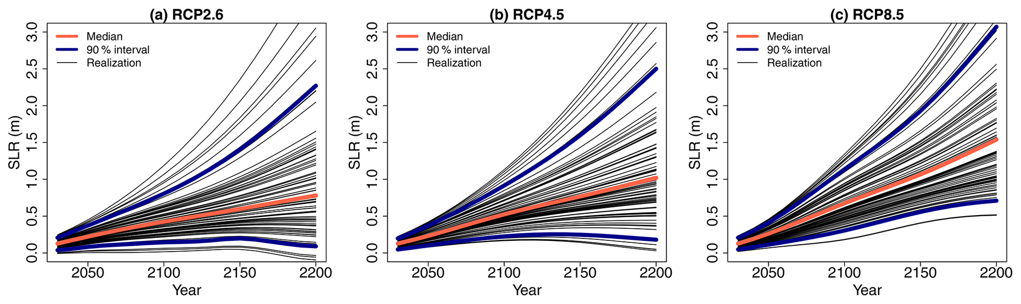
Figure 4Future projection of regional SLR for 3 different RCP scenarios. The red line indicates the median, and the blue lines indicate the bounds of the 90 % confidence interval provided by Kopp et al. (2014). The different black lines correspond to a subset of 75 randomly generated time series using the procedure described in Sect. 2.3.
In summary, time series of SLRRCP are defined by combining an RCP scenario with a percentile level pSLR (ranging between 0 and 1). Figure 4 shows the projections for the three RCP scenarios considering pSLR = 50 % (median in red) and pSLR = 5 % and 95 % (90 % interval in blue). To account for the uncertainty in SLRRCP, the following random sampling procedure is proposed: (1) a percentile level pSLR is randomly and uniformly sampled between 0 and 1, and (2) the inverse of the empirical cumulative distribution estimated based on the data by Kopp et al. (2014) is then used to sample a time series of projected SLRRCP(t) values for a given RCP scenario; i.e. the same pSLR level is considered over the period 2030–2200 (with a time step of 10 years). See some examples in Fig. 4 of random realizations following this procedure.

Figure 5Flowchart of the procedure. The sections describing the methods/data are indicated in grey next to the boxes.
3.1 Overall procedure
The objective is twofold. First, we aim to estimate the flooding probability Pf defined as the probability that the median value mY (related to wave stochasticity; see Sect. 2.1) of the inland water volume Y induced by the flood exceeds a given threshold YC, namely
where E(.) is the expectation operator, I{A} is the indicator function which takes up 1 if A is true and 0 otherwise and denotes the hydrodynamic simulator f(.) described in Sect. 2 which takes the vector x of offshore forcing conditions as inputs to compute mY by conducting nr = 20 repeated numerical simulations. Second, we aim to quantify the contributions of each offshore forcing conditions to the occurrence of the flooding event defined by {mY>YC}. The different steps of the procedure are depicted in Fig. 5 and described below.
Step 1. To overcome the large computation time cost to estimate mY, we set up a metamodel (see details in Sect. 3.3) which is trained using a number n of inputs and the corresponding median value (computed by running the hydrodynamic simulator nr times). As a metamodel, we opt for the Gaussian process (GP) regression method (Williams and Rasmussen, 2006), whose implementation and validation are described in Sect. 3.2. One advantage of the GP is that it is capable of accounting for the metamodel error, i.e. the uncertainty related to the approximation of the true numerical model by a metamodel that is built using only a finite number of simulation results (see Step 3).
Step 2. Using the database of hindcasts described in Sect. 2.2, a multivariate extreme value analysis is conducted to randomly generate a large number N of “extreme but realistic” random realizations x of the scalar offshore meteo-oceanic conditions via a Monte Carlo procedure (Sect. 3.3). The effect of SLR is accounted for by following the random procedure described in Sect. 2.3.
Step 3. Using the validated GP metamodel, Pf is estimated using the N randomly generated realizations of the offshore conditions. The respective contribution of the different offshore forcing conditions to the occurrence of the flooding event {mY>YC} is quantified using the tools of GSA (Sect. 3.4). We account for two sources of uncertainty in the estimation procedure, namely the Monte Carlo sampling and the GP error, by replicating B times the estimation within a Monte Carlo-based approach described in Sect. 3.5.
3.2 Step 1: Gaussian process metamodel
Let us consider the set of n training data . In the context of GP modelling (also named as kriging, Williams and Rasmussen, 2006), we assume, prior to any numerical model run, that is a realization of a GP (MY(x)) with
-
a mean (also named trend) (where gj is fixed basis functions and βj is the regression coefficients of the k input variables)
-
a stationary covariance function (named kernel) written as with σ2 the variance parameter.
For new offshore forcing conditions x∗, the predictive probability distribution follows a GP with mean μGP(x∗) and variance V(x∗) defined using the universal kriging equations (e.g. Roustant et al., 2012) as follows:
where ; C is the covariance matrix between the points , whose element is ; c(x∗) is the vector composed of the covariance between MY(x∗) and the points ; g(x∗) is the vector of trend functions values at x∗; is the experimental matrix; the best linear estimator of β is ; and by assuming to be stationary (Williams and Rasmussen, 2006).
The n numerical experiments used to train the GP model are selected by combining two techniques: (1) for the extreme values, we use the approach developed by Gouldby et al. (2014) by means of a clustering algorithm applied to a large dataset of extreme forcing conditions, with this database being constructed through a combination of Monte Carlo random sampling and multivariate extreme value analysis performed on the database of hindcast conditions described in Sect. 2.2, and (2) for low and moderate values, we use the conditioned Latin hypercube sampling procedure of Minasny and McBratney (2006), for which the reader can refer to Rohmer et al. (2020) for further details on the implementation for the site of interest here.
To validate the assumption of replacing the true numerical simulator by the kriging mean (Eq. 2a), we measure whether the GP model is capable of predicting “yet-unseen” input configurations, i.e. samples that have not been used for training. This can be examined by using a K-fold cross-validation approach (e.g. Sect. 7.10 of Hastie et al., 2009). To do so, the training data are first randomly split into K roughly equal-sized parts (named folds). For the kth fold, we fit the GP model to the other K−1 parts of the data and calculate the prediction error of the fitted model when predicting the kth part of the data. We do this at each iteration of the procedure and compute the coefficient of determination denoted as follows:
where n(k) is the size of the kth part of the data (), xi is the ith element of the kth part of the data, is the prediction at xi using the GP model fitted using the kth part of the data removed (i.e. the GP model is fitted using K−1 parts of the data), is the median value of Y related to xi computed using the modelling procedure of Sect. 2 and is the average value of the numerically computed median values for the kth part of the data. A coefficient close to 1.0 indicates that the GP model is successful in matching the new observations that have not been used for the training. The spread of further informs on the stability of the predictive capability across the k folds.
3.3 Step 2: multivariate extreme value analysis
The flooding probability (Eq. 1) is computed via a Monte Carlo sampling approach based on the random generation of the offshore conditions. To do so, two classes of offshore conditions are considered: “amplitude” random variables X = (SWL, Hs, U), which can take up very large values, and covariates Xc = (Tp, Dp, Du), which are dependent on the values of the amplitude variables. Considering amplitude variables, a multivariate extreme value analysis (Coles, 2001) is conducted to extrapolate their joint probability density to extreme values by taking into account the dependence structure. A three-step approach is performed as follows.
Step 1. Fitting of the marginals of amplitude variables through the combination of the empirical distribution, below a suitable high threshold u, and of the generalized Pareto distribution (GPD), above the selected threshold u (Coles and Tawn, 1991), using the method of moments. The threshold value u of the amplitude random variables is selected using the Bayesian cross-validation procedure developed by Northrop et al. (2017).
Step 2. The dependence structure of the amplitude variables is modelled using the approach of Heffernan and Tawn (2004). Let us denote the vector of all variables (with prior transformation onto common standard Laplace margins, Keef et al., 2013) except the ith variable . A multivariate non-linear regression model is set up as follows:
where > υ (i.e. having large values), a and b are parameters vectors (one value per parameter for each pair of variables), υ is a threshold that is selected using the diagnostic tools described in Heffernan and Tawn (2004; Sect. 4.4), and W is a vector of residuals. The model is adjusted using the maximum-likelihood method assuming that the residuals W are Gaussian and independent of Xi with a mean and variance to be calculated. Once fitted, a Monte Carlo simulation procedure is used to randomly generate realizations of the amplitude variables X (after transformation back on physical scales) by following the algorithm described in Sect. 4.3 of Heffernan and Tawn (2004).
Step 3. Based on the generated dataset of amplitude variables, the random samples for the directional covariates Dp and Du are generated by using the empirical distribution conditional on the values of Hs and of U, respectively. The peak period Tp values are generated by following the approach described by Gouldby et al. (2014) based on a regression model using wave steepness conditional on Hs.
3.4 Step 3: global sensitivity analysis and Shapley effect
The objective is to investigate the influence of the offshore conditions with respect to the occurrence of the event mY>YC in relation to the flooding probability defined in Eq. (1). To do so, we opt for the GSA approach based on the Shapley effects proposed by Idrissi et al. (2021) and applied in the field of reliability assessment. For sake of presentation clarity, we first present the Shapley effect by considering the situation where the variable of interest is a scalar variable (Sect. 3.4.1). Second, we present the adaptation in relation to the problem of flooding probability (Sect. 3.4.2).
3.4.1 Shapley effect for a scalar variable of interest
Among all the GSA methods (Iooss and Lemaître, 2015), we opt for a variance-based GSA, denoted VBSA (Saltelli et al., 2008), which aims to decompose the total variance of the scalar variable of interest denoted here Z into the respective contributions of each uncertainty, with this percentage being a measure of sensitivity.
Recall that f(.) is the numerical simulator. Consider the k-dimensional vector x as a random vector of k random input variables Xi () related to the different offshore forcing conditions. Then, the variable of interest Z=f(x) is also a random variable (as a function of a random vector). VBSA determines the part of the total unconditional variance Var(Z) of the output Z resulting from each input random variable Xi. Formally, VBSA relies on the first-order Sobol' indices (ranging between 0 and 1), which can be defined as
where E(.) is the expectation operator.
When the input variables are independent, the index Si corresponds to the main effect of Xi, i.e. the share of variance of Y that is due to a given Xi. The higher the influence of Xi is, the lower the variance is when fixing Xi to a constant value, hence the closer Si is to 1.
When dependence/correlation exists among the input variables (as is the case in our study; see Sect. 2.2), a more careful interpretation of Eq. (5) should be given: in this situation, a part of the sensitivity of all the other input variables correlated with the considered variable contributes to Si, which cannot be interpreted as the proportion of variance reduction related to fixing Xi. To overcome this difficulty, an extension of the Sobol' indices has been proposed in the literature, namely the Shapley effects (Owen, 2014; Iooss and Prieur, 2019; Song et al., 2016). The advantage of these effects is to allocate a percentage of the model output's variance to each input variable which includes not only the individual effect but also the higher-order interaction and, above all, the (statistical) dependence. By summing to the total variance (i.e. the sum of all normalized effects is one) and by being non-negative, the Shapley effects allow for an easy interpretation (Iooss and Prieur, 2019).
Formally, the sensitivity indices are defined based on the Shapley value (Shapley, 1953) that is used in game theory to evaluate the “fair share” of a player in a cooperative game; i.e. it is used to fairly distribute both gains and costs to multiple players working cooperatively. Formally, a k-player game with the set of players is defined as a real-valued function that maps a subset of K to its corresponding cost so that c(A) is the cost that arises when the players in the subset A of K participate in the game. The Shapley value of player i with respect to c(.) is defined as
where |A| is the size of the set A.
In the context of GSA, the set of players K can be seen as the set of inputs of f(.), and c(.) can be defined so that for A⊆K, c(A) measures the variance of Z caused by the uncertainty of the inputs in A. Owen (2014) proposed the so-called “closed Sobol' indices” as the cost function:
where XA is the subset of inputs selected by the indices in A, namely ().
The Shapley effect can thus be defined as
3.4.2 Shapley effect for the occurrence of a flooding event
In our study, the Shapley effect cannot be directly applied because we are not interested in the variance of a scalar variable (denoted Z in Sect. 3.4.1) but in the occurrence of an exceedance event in relation to the flooding probability defined in Eq. (1). Thus, we rely on the adaptation of the Shapley effect to this case, namely “target Shapley effects” proposed by Idrissi et al. (2021) as follows:
where .
The target Shapley effects TShi can be interpreted as a percentage of the variance of the indicator function allocated to the input Xi and measures the influence of the input to the occurrence of the flooding event (defined by the exceedance of the median value mY of Y above YC).
3.5 Estimation procedure
In practice, the Shapley effects defined in Eq. (9) are evaluated using a “given data” approach, i.e. through the post-processing of the Monte Carlo-based results using the nearest-neighbour search-based estimator developed by Broto et al. (2020) with the “sobolshap_knn” function of the R package “sensitivity” (Iooss et al., 2021) using five neighbours and a pre-whitening of the inputs with the procedure by Kessy et al. (2018).
In this estimation, two major sources of uncertainty should be accounted for, namely the Monte Carlo sampling and the GP error (related to the approximation of the true numerical model by a GP built using a finite number of simulation results). This is done as follows.
Step 1. A set of N random realizations of the forcing conditions are generated using the methods described in Sect. 3.3.
Step 2. For the N randomly generated forcing conditions, a conditional (stochastic) N-dimensional simulation of the GP (knowing the training data) is generated using Eqs. (2a) and (2b), and the N values of mY are estimated.
Step 3. Using the set of N values of mY, the flooding probability is estimated using Eq. (1), and the Shapley effects are computed using the nearest-neighbour search-based estimator.
Steps 1 to 3 are repeated B times to generate a set of B Shapley effects (one effect per forcing condition). The variability in these estimates then reflects the use of different sets of random samples (sampling error) and the use of different conditional simulations of the GP (GP error).
In this section, we apply the procedure described in Sect. 3 to partition the uncertainty in the occurrence of the event {mY>YC} by considering a base (reference) case defined by a volume threshold YC = 2000 m3, which corresponds to a flooding event of moderate magnitude (see Fig. 2b), and by the effect of SLR for the RCP4.5 scenario (see Fig. 4b). The latter RCP scenario is selected because it approximately corresponds to the intended nationally determined contributions submitted in 2015 ahead of the Paris Agreement approval (UNFCCC, 2016). The impact of these assumptions is further discussed in Sect. 5.
4.1 Step 1: GP metamodel training and validation
Using the approach described in Sect. 3.2, we first select 100 offshore conditions used as inputs to the modelling chain to calculate the corresponding median value mY (green circles in Fig. 3). In addition, 44 extra cases (squares in Fig. 3) were defined using the set of high-tide conditions that were randomly generated for the design of the early-warning system at Gâvres (Sect. 2.5 of Idier et al., 2021). These conditions were used as inputs of the metamodel implemented by Rohmer et al. (2020) to predict the flooding-induced water height at the observation point P (Fig. 1b), which is a critical location with respect to seawater entry during a storm event; the conditions leading to a positive water height were then selected. In total, n=144 computer experiments were performed.
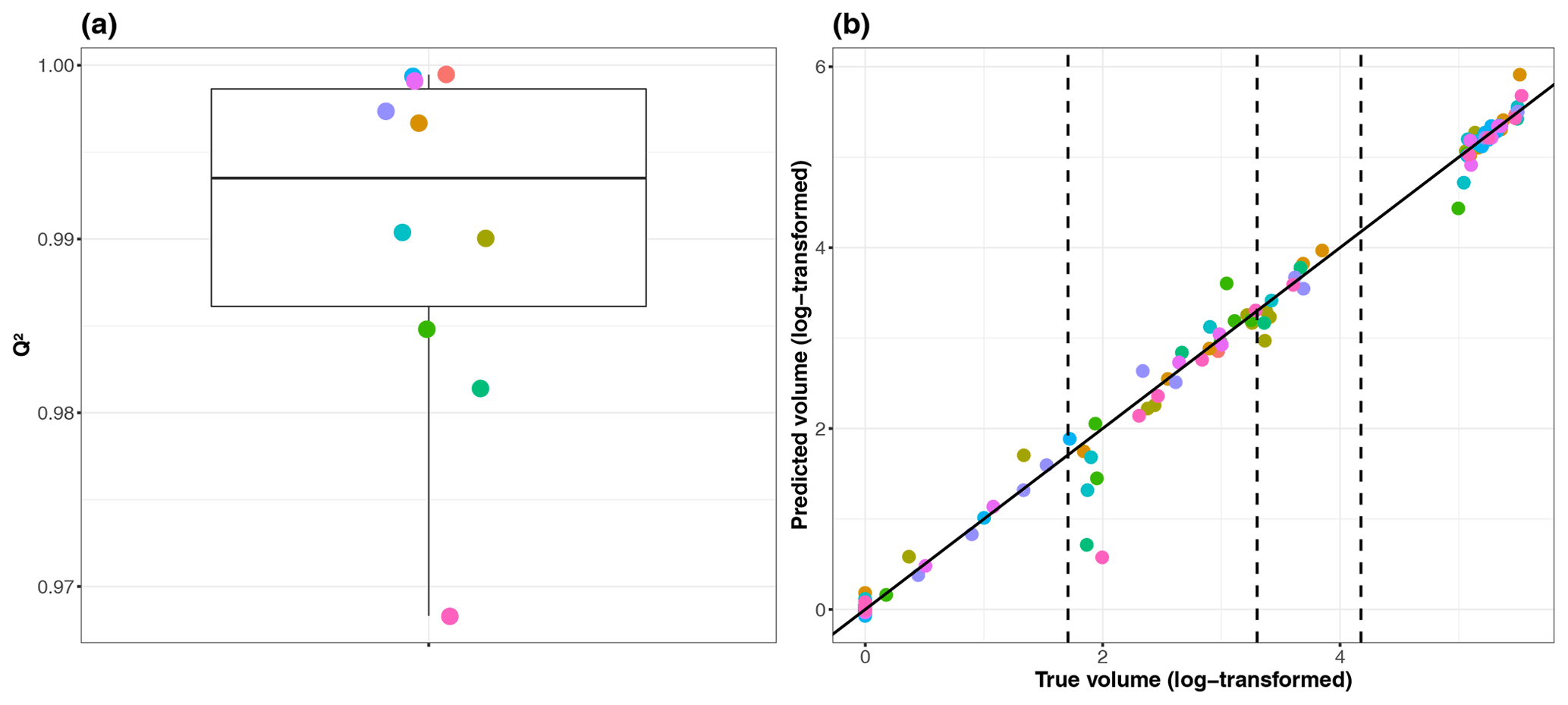
Figure 6(a) Boxplot of performance indicator values Q2 (for the 10 folds of the cross-validation procedure). Each colour indicates the number index of the corresponding fold. (b) Comparison between the volume (log10-transformed) estimated using the “true” numerical simulator and the ones predicted using the GP model for each of the 10 folds of the cross-validation procedure. The closer the dots are to the first bisector, the more satisfactory the predictive capability of the trained GP model is. The vertical dashed lines indicate the threshold YC (log10-transformed) used in the study (50, 2000 and 15 000 m3).
The GP model is trained by assuming a linear trend μ and a Matérn kernel model in Eqs. (2a) and (2b) and using a maximum-likelihood estimation of the GP parameters (e.g. Roustant et al., 2012). The GP metamodel is validated using a 10-fold cross validation procedure as described in Sect. 3.2. Due to the highly skewed distribution of mY, we use a logarithm transformation, i.e. log10(mY+1). The cross-validation procedure shows a high predictive capability of the trained metamodel with a median value Q2 ≈ 99.35 % (calculated across the 10 folds) and a small spread (as shown by the small inter-quartile width of 1.25 %; see Fig. 6a). Our preliminary tests also showed that the logarithm transformation improved the predictive capability with an increase in Q2 of 10 %. The scatterplot in Fig. 6b confirms that the predictive capability of the trained GP model is very satisfactory (the dots almost align along the first bisector). However, we can notice some deviations, in particular in the vicinity of the volume threshold defining minor flooding event, i.e. . This provides a clear justification for accounting for the GP error in the GSA results by following the procedure described in Sect. 3.5.
4.2 Step 2: multivariate extreme value analysis
We use the database of hindcast conditions described in Sect. 2.2 to extract > 80 000 offshore forcing conditions characterized by (SWL, Hs, U, Tp, Dp and Du) taken at the time instant of the high tide (blue dots in Fig. 3). Following Step 1 described in Sect. 3.3, the extracted data are used to fit the marginals of the amplitude variables using the GPD distribution with the selected threshold values of = 3.59 m, uSWL = 2.37 m and uU = 9.51 m s−1 by applying the procedure of Northrop et al. (2017) over the quantile range [85.0 %, 99.9 %]. The goodness of GPD fit is also checked by analysing the different diagnostic plots provided in Sect. S2.
Following Step 2 in Sect. 3.3, the dependence is modelled with the selected threshold υ of Eq. (4) set up at 0.97 (expressed as a probability of non-exceedance). On this basis, the Monte Carlo simulation procedure described by Heffernan and Tawn (2004) is used to randomly generate N = 50 000 events using the R package “texmex” (Southworth et al., 2020). Based on the generated dataset, the corresponding covariate values are also generated (Step 3 in Sect. 3.3). Figure 3 provides an overview of the randomly generated samples (red dots) for the amplitude variables and for the covariates. The visual analysis of this figure confirms the moderate-to-large statistical dependence between the sampled forcing conditions (if they were independent, no structure would be noticed) with satisfactory reproduction of the structure of the observations (blue dots). The examination of the (a,b) parameters of the dependence model (as defined in Eq. 4) indicates a non-negligible positive strength of dependence in the class of asymptotic independence (Sect. S1) in agreement with the analysis made on the hindcast database (Sect. 2.2).
4.3 Step 3: uncertainty partitioning over time
The N = 50 000 randomly generated forcing conditions in addition to the random SLR time series (see some examples in Fig. 4) are used as inputs of the validated GP models to evaluate the time evolution of Pf for YC = 2000 m3 given for RCP4.5 (Fig. 7). Preliminary convergence analysis showed that 50 000 Monte Carlo samples were sufficient to reach stable results; this is also shown by the very small uncertainty band's width in Fig. 7 (see in particular the inserted plot) defined by the lower and upper bounds computed using B=50 replicates of the estimation procedure (described in Sect. 3.5). Figure 7 shows that Pf increases over time in a non-linear manner and reaches values of ∼ 1.5 % in the long term by 2100 and ∼ 22 % in the very long term by 2200.

Figure 7Time evolution of the probability of the event given SLR projections for the scenario RCP4.5. The inserted figure indicates the very small uncertainty band's width, whose limits are the lower and upper bounds computed using B=50 replicates of the estimation procedure (Sect. 3.5) accounting for GP and sampling error.
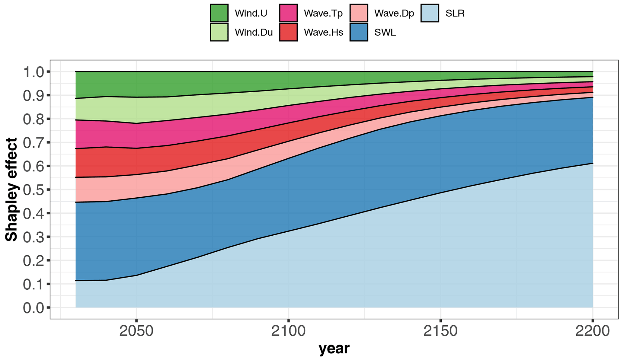
Figure 8Time evolution of the Shapley effects, relative to the occurrence of the event given SLR projections for the scenario RCP4.5, estimated by computing the median value from B=50 replicates of the estimation procedure (Sect. 3.5) accounting for GP and sampling error.
Table 1Shapley effects relative to the occurrence of the event given SLR projections for the scenario RCP4.5, estimated by computing the median value from B=50 replicates of the estimation procedure (Sect. 3.5) accounting for GP and sampling error. The numbers in brackets correspond to the minimum and maximum value computed from the B=50 replicates.
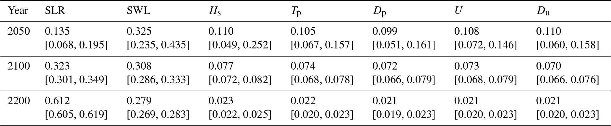
The Shapley effects for the flooding event {mY>2000 m3} were evaluated using the 50 000 GP model evaluations using B=50 replicates of the estimation procedure (Sect. 3.5) accounting for GP and sampling error. Preliminary convergence analysis showed us that 50 000 samples were sufficient to reach low uncertainty estimates as shown at given time instants in Table 1. This also confirms that both error sources (GP and sampling) have a small influence. Figure 8 depicts the time evolution of the Shapley effects, which measure the influence of the inputs on the occurrence of the flooding event.
Several effects are noticed as follows.
-
The influence of SLR increases over time with a non-negligible contribution of ∼ 13.5 % even in the short term (< 2050) until reaching ∼ 32 % in the long term (2100) by following a relatively steep evolution (with an increase of almost 140 % from 2020 to 2100).
-
After 2100, SLR contribution continues to increase until reaching ∼ 61 % in the very long term (2200). This means that by 2200, SLR dominates the cumulative contributions of all remaining uncertainties.
-
In the short term, the major contributor corresponds to SWL. The Shapley effect is of ∼ 32 %, while the remaining forcing conditions have contributions of the order of ∼ 10 %–11 %. By 2100, SLR Shapley effect exceeds the one of SWL.
-
Over time, the contributions of all forcing conditions (except SLR) decrease (to compensate the SLR increase because the sum of all Shapley effects is one). We note that by 2075 (2150, respectively), the cumulative contribution of both SLR and SWL represents ∼ 50 % (75 %, respectively) of the variance.
-
After 2100, the Shapley effects of the wave and wind characteristics (Hs, Tp, Dp, U, Du) reach low levels (∼ 7 %–8 %), and after 2150, the contributions are < 3 %, which provides strong evidence of their negligible role in the very long term; i.e. their individual effect and their dependence and their interactions with the other variables are almost zero. This effect would not have been revealed if “traditional” sensitivity analysis (using Sobol' indices) had been used, because the strong dependence among the inputs would not have been accounted for (Sect. S3).
In this section, we first investigate whether the conclusions on the uncertainty partitioning (Sect. 4.3) might change depending on some key modelling choices (Sect. 5.1). Second, we further discuss the implications of different limitations for both the numerical and the statistical modelling (Sect. 5.2).
5.1 Influence of key modelling choices
The uncertainty partitioning in Sect. 4.3 underlines the key influence of SLR on the occurrence of the event . We investigate here to which extent alternative assumptions underlying our approach might change the above-described conclusions, namely the following.
-
The volume threshold YC used to define when a flooding event occurs. The analysis was performed given a threshold YC = 2000 m3 related to a moderate flooding event (Fig. 2), and it is re-conducted here by, respectively, focusing on minor and very large flooding events defined for YC = 50 and 15 000 m3 (as illustrated in Fig. 2).
-
The choice in the RCP scenario to constrain the SLR projections described in Sect. 2.3. The analysis was conducted given the RCP4.5 scenario, i.e. given a scenario related to relatively moderate SLR magnitude (Fig. 4b), compared to RCP8.5 in particular (Fig. 4c). The analysis is here re-conducted for the RCP2.6 and 8.5 scenarios.
-
The choice of the DEM. This modelling choice is known to highly influence the results (see e.g. Abily et al., 2016), and we investigate to which extent an alternative DEM might change the sensitivity analysis results by considering DEM 2008 (with the same resolution of 3 m as DEM 2015), which corresponds to the conditions before the major flooding event of Johanna in 2008, i.e. prior to the protective measures relying on the raise of the dykes in the aftermath of this event.
-
The choice of the summary statistics to account for wave stochasticity. The analysis was conducted by using the median value mY of Y as described in Sect. 2.1. The analysis is here re-conducted using the first quartile (denoted Q25) or the third quartile (denoted Q75).
For each analysis, the corresponding assumption was changed, and the whole analysis (described in Sect. 3.1) was re-conducted, i.e. (1) new hydrodynamic simulations, (2) training of new GP models (the predictive capability is confirmed as shown in Sect. S5), and (3) GP-based estimate of the flooding probability and of the Shapley effects within a Monte Carlo-based simulation procedure (Sect. 3.5).
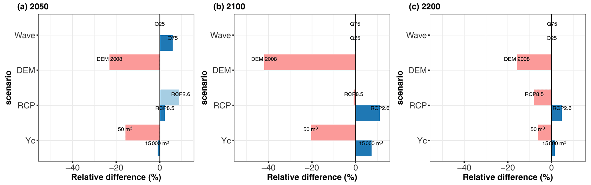
Figure 9Relative differences of the Shapley effect for SLR (using the median value computed for B=50 replicates of the estimation procedure) with respect to the base case at different time horizons (2050 in a, 2100 in b and 2200 in c) considering alternative modelling choices for the volume threshold YC, the RCP scenario, DEM and the summary statistics of wave stochasticity.
Figure 9 summarizes these results and shows that the SLR effect both depends on our modelling choices and on the considered time horizon. Before 2100, it is strongly influenced by the DEM (Fig. 9a and b), with a reduction in SLR influence by −40 % to −20 %. The differences in the short/long term were expected because DEM 2008 presents some sectors of lower topographic elevation of coastal defences (Sect. S4) compared to DEM 2015 (in particular on the south-eastern sector, which is highly exposed to storm impacts). A more detailed analysis of the uncertainty contribution (Sect. S5) shows that the decrease in SLR influence for DEM 2008 goes in parallel with higher contributions of wave characteristics, hence confirming that drivers of flooding change depending on the DEM, with the sectors with lower topographic elevation having a higher sensitivity to wave-induced flooding, i.e. overtopping at least until 2100.
The second major driver of SLR influence is the choice in the threshold. Reducing its value (case YC = 50 m3) reduces SLR contribution, which is directly translated into an increase in SWL contribution (Sect. S5). This SLR–threshold relation directly reflects how SLR acts on the flooding likelihood: it acts as an “offset”, which means that it induces a higher seawater level at the coast, hence a higher likelihood of flooding. Thus, the lower the threshold value is, the lower the necessary SLR magnitude to induce flooding is, hence the lower influence is. This threshold also means that results presented in Fig. 8 are specific to our case study in Gâvres. In other settings where flooding is dominated by overflow, breaching or overtopping with another threshold, the partition of uncertainties is expected to be different.
The third driver of SLR influence is the choice in the RCP scenario. Before 2100, making the assumption of the RCP2.6 scenario leads to an increase in SLR influence, up to ∼ 10 %. It is only in the very long term (beyond 2100) that assuming the RCP8.5 scenario leads to a reduction in the SLR influence. Like for YC, this is the offset effect of SLR that influences the most: for RCP8.5, the mode of the SLR distribution (in red in Fig. 4c) exceeds the one of the other scenarios after 2100 and can induce a high seawater level at the coast, hence potentially a water volume value close to YC = 2000 m3 and a higher flooding likelihood. This means that SLR values sampled around the mode will impact the occurrence of the flooding event (and the flooding probability) less because a small SLR offset is here necessary to trigger the flooding event. This is not the case for the two alternative RCP scenarios because the mode is of lower magnitude and any SLR values sampled above it will have a key impact on the flooding occurrence.
Finally, the uncertainty partitioning is shown to be very slightly influenced by the choice of the summary statistics for the wave stochasticity (Fig. 9) especially in the long term after 2100. This result differs from the one of Idier et al. (2020b), who showed the importance of this effect is comparable to the one of SLR value as long as the still water level remains smaller than the critical level, above which overflow occurs. The differences between both studies may be explained by the differences in the procedure. Idier et al. (2020b) analysed this effect for two specific past storm events, whereas our study covers a large number of events by randomly sampling different offshore forcing conditions. To conclude on this effect (relative to the others), further investigations are thus necessary and could benefit for instance from recent GSA for stochastic simulators (Zhu and Sudret, 2021).
5.2 Limitations
While the analysis in Sect. 5.1 covers the main modelling choices of our procedure, we acknowledge that several aspects deserve further improvements.
Regarding the modelling of the flood processes, one of our main assumptions is to perform simulations with steady-state offshore forcing conditions, i.e. without accounting for the time evolution of the forcing conditions around the high tide (Sect. 2.1). First, this choice was guided by the computational budget that could be afforded to account for wave stochasticity via repeated numerical simulations. A total of 144 × 20 = 2880 numerical simulations were performed here for our analysis: such a large number of simulations would be difficult to achieve using non-stationary numerical simulations because a single run takes about 3 d of computation on 48 cores. Second, Idier et al. (2020b) showed, for two historical storm events, that the value of Y remains of the same order of magnitude between a steady-state and a non-stationary simulation. Therefore, the temporal effect is expected to only moderately influence our conclusions regarding uncertainty partitioning. If, however, other flooding indicators are chosen (e.g. total flooded area or water height at a given inland location), i.e. indicators that are more sensitive to the time evolution of offshore conditions, non-stationary simulations are mandatory. In this case, time dimension should be accounted for at different levels of the procedure: (1) metamodelling with functional inputs (e.g. using the procedure developed by Betancourt et al., 2020), (2) integrating additional variables in the multivariate extreme value analysis like event duration and event spacing (e.g. Callaghan et al., 2008), and (3) randomly generating time-varying forcing conditions (e.g. using the stochastic emulator used by Cagigal et al., 2020, to force ensemble long-term shoreline predictions).
Regarding the physical drivers of flooding, the analysis was focused on marine flooding by considering the joint wave–wind–sea level effects, but additional processes are also expected to play a role in driving the compound flooding, like river discharge (in particular with the proximity of the Blavet River1 on the study area) or rainfall. Including additional drivers is made here feasible by the flexibility of the approach of Heffernan and Tawn (2004) for analysing high-dimensional extremes. This was shown in particular by Jane et al. (2020), who also highlighted the value of copula-based approaches, such as vine copula. An avenue for future research could include the comparison of different approaches for multivariate extreme value analysis, i.e. a type of modelling uncertainty on top of the uncertainties in the parametrization and in the threshold selection of these techniques (e.g. Northrop et al., 2017).
Finally, regarding the drivers' evolution under climate change, we used the projections from Kopp et al. (2014). These are generally consistent with the latest IPCC sea level projections presented in the Special Report on Ocean and Cryosphere in a Changing Climate (Oppenheimer et al., 2019). The range of these projections is also similar with medium-confidence projections provided by the Sixth Assessment Report of the IPCC, at least until 2100 (Fox-Kemper et al., 2021). Yet, the highest quantiles may not represent the possibility of marine ice-sheet collapse in Antarctica well (De Conto et al., 2021). The lowest quantiles of the projections of Kopp et al. (2014) need to be considered even more cautiously, with the 17 % quantile being a reasonable minimal estimate (named the low-end scenario; see e.g. Le Cozannet et al., 2019b) given the scientific evidence available today. Integrating these updated data is a line of future work whose implementation will benefit from the low computational budget of the metamodels. In addition, one of our main assumptions regarding SLR is that only SWL is impacted, while the current wave and wind climate remains unchanged in the future. This assumption should be reconsidered in future work in particular in light of recent projections (see e.g. Morim et al., 2020, for wave and Outten and Sobolowski, 2021, for wind) and by taking advantage of recent advances in stochastic modelling like that used by Cagigal et al. (2020).
At the macrotidal site of Gâvres (French Brittany), we have estimated the time evolution of the flooding probability defined so that the median value mY (related to wave stochasticity) of the inland water volume Y induced by the flooding exceeds a given threshold YC. For moderate flooding events (with YC = 2000 m3), the flooding probability rapidly reaches ∼ 1.5 % by 2100 and (quasi-)linearly increases until ∼ 22 % in the very long term (by 2200). By relying on Shapley effects, our study underlines the key influence of SLR on the occurrence of the event mY>YC regardless of the YC value together with a small-to-moderate contribution of wave and of wind characteristics and even of negligible importance in the very long term for the covariates Dp, Du and Tp. This growing influence of SLR (and then of the climate scenarios over the 21st and 22nd centuries) was expected and is a feature that would be observed across many coastal sites around the world. Yet, the time evolution of the flood probability (and associated uncertainty) remains site-specific, i.e. mostly related to the particular conditions that generate flooding in each coastal area, and could not have been quantified without the implementation of the proposed procedure.
The analysis of the main uncertainties in the estimation procedure (Monte Carlo sampling and GP error) shows a minor impact here, which is a strong indication that the combined GP–Shapley effect approach is a robust tool worth integrating into the toolbox of coastal engineers and managers to explore and characterize uncertainties related to compound coastal flooding under SLR. However, to reach an operative level, two key aspects deserve further investigation: (1) the optimized computational effort with appropriate metamodelling techniques (e.g. Betancourt et al., 2020, for functional inputs and Zhu and Sudret, 2021, for stochastic simulators) combined with an advanced Monte Carlo sampling scheme (like importance sampling, Demange-Chryst et al., 2022) and (2) the capability to assess the impact of alternative modelling choices (extreme value modelling and numerical modelling, in addition to those described in Sect. 5.1) on the sensitivity analysis, i.e. a problem named “sensitivity analysis of sensitivity analysis” by Razavi et al. (2021). This latter aspect requires a more general framework to incorporate multiple levels of uncertainty, i.e. a first level that corresponds to the forcing conditions, a second level that is related to the modelling choices and a third level that is related to the stochastic nature of our numerical model (related to wave stochasticity).
Codes are available upon request to the first author.
All references of the data used to develop the numerical and the statistical models presented are included in the paper. The authors are available for any specific requirement.
The supplement related to this article is available online at: https://doi.org/10.5194/nhess-22-3167-2022-supplement.
JR, DI and GLC designed the concept. JR, DI and FB set up the methods. JR, DI, RT, GLC and FB set up the numerical experiments. DI performed the numerical analyses with the hydrodynamic model. RT and GLC pre-processed and provided the projection data. JR undertook the statistical analyses. JR wrote the manuscript draft, DI, RT, GLC and FB reviewed and edited the manuscript.
The contact author has declared that none of the authors has any competing interests.
Publisher's note: Copernicus Publications remains neutral with regard to jurisdictional claims in published maps and institutional affiliations.
The authors thank the ANR (Agence Nationale de la Recherche) for its financial support to the RISCOPE (Risk-based system for coastal flooding early warning) project (grant no. ANR-16-CE04-0011). We thank Fabrice Gamboa (IMT, Institut de Mathématiques de Toulouse), Thierry Klein (IMT and ENAC, Ecole Nationale de l'Aviation Civile), Rodrigo Pedreros (BRGM) and Bertrand Iooss (EDF, IMT) for fruitful discussions. We are grateful to Panagiotis Athanasiou and the two anonymous reviewers, whose comments improved the paper.
This research has been supported by the Agence Nationale de la Recherche (grant no. ANR-16-CE04-0011). This research was partly conducted with the support of the CIROQUO consortium in applied mathematics (https://doi.org/10.5281/zenodo.6581217), gathering partners in technology and academia in the development of advanced methods for computer experiments.
This paper was edited by Animesh Gain and reviewed by Panagiotis Athanasiou and two anonymous referees.
Abily, M., Bertrand, N., Delestre, O., Gourbesville, P., and Duluc, C. M.: Spatial Global Sensitivity Analysis of High Resolution classified topographic data use in 2D urban flood modelling, Environ. Modell. Softw., 77, 183–195, 2016.
Anderson, B., Borgonovo, E., Galeotti, M., and Roson, R.: Uncertainty in climate change modelling: can global sensitivity analysis be of help?, Risk Anal., 34, 271–293, 2014.
Ardhuin, F., Rogers, W. E., Babanin, A. V., Filipot, J., Magne, R., Roland, A., Van der Westhuysen, A., Queffeulou, P., Lefevre, J., Aouf, L., and Collard, F.: Semiempirical dissipation source functions for ocean waves. Part I: Definition, calibration, and validation, J. Phys. Oceanogr., 40, 917–941, 2010.
Athanasiou, P., van Dongeren, A., Giardino, A., Vousdoukas, M. I., Ranasinghe, R., and Kwadijk, J.: Uncertainties in projections of sandy beach erosion due to sea level rise: an analysis at the European scale, Sci. Rep., 10, 11895, https://doi.org/10.1038/s41598-020-68576-0, 2020.
Bamber, J. L. and Aspinall, W. P.: An expert judgement assessment of future sea level rise from the ice sheets, Nat. Clim. Change, 3, 424–427, 2013.
Betancourt, J., Bachoc, F., Klein, T., Idier, D., Pedreros, R., and Rohmer, J.: Gaussian process metamodeling of functional-input code for coastal flood hazard assessment, Reliab. Eng. Syst. Safe., 198, 106870, https://doi.org/10.1016/j.ress.2020.106870, 2020.
Bevacqua, E., Vousdoukas, M. I., Zappa, G., Hodges, K., Shepherd, T. G., Maraun, D., Mentaschi, L., and Feyen, L.: More meteorological events that drive compound coastal flooding are projected under climate change, Communications Earth & Environment, 1, 1–11, 2020.
Broto, B., Bachoc, F., and Depecker, M.: Variance reduction for estimation of Shapley effects and adaptation to unknown input distribution, SIAM/ASA Journal of Uncertainty Quantification, 8, 693–716, 2020.
Cagigal, L., Rueda, A., Anderson, D. L., Ruggiero, P., Merrifield, M. A., Montaño, J., Coco, G., and Méndez, F. J.: A multivariate, stochastic, climate-based wave emulator for shoreline change modelling, Ocean Model., 154, 151–184, 2020.
Callaghan, D. P., Nielsen, P., Short, A., and Ranasinghe, R. W. M. R. J. B.: Statistical simulation of wave climate and extreme beach erosion, Coastal Engineering, 55, 375–390, 2008.
Chaumillon, E., Bertin, X., Fortunato, A. B., Bajo, M., Schneider, J.-L., Dezileau, L., Walsh, J. P., Michelot, A., Chauveau, E., Créach, A., Hénaff, A., Sauzeau, T., Waeles, B., Gervais, B., Jan, G., Baumann, J., Breilh, J.-F., and Pedreros, R.: Storm-induced marine flooding: Lessons from a multidisciplinary approach, Earth-Sci. Rev., 165, 151–184, 2017.
Coles, S.: An Introduction to Statistical Modeling of Extreme Values, Springer Verlag, London, 2001.
Coles, S., Heffernan, J., and Tawn, J.: Dependence Measures for Extreme Value Analyses, Extremes, 2, 339–365, 1999.
Coles, S. G. and Tawn, J. A.: Modelling extreme multivariate events, J. Roy. Stat. Soc. Ser. B Met., 53, 377–392, 1991.
De Conto, R. M., Pollard, D., Alley, R. B., Velicogna, I., Gasson, E., Gomez, N., Sadai, S., Condron, A., Gilford, D. M., Ashe, E. L., and Kopp, R. E.: The Paris Climate Agreement and future sea-level rise from Antarctica, Nature, 593, 83–89, 2021.
Demange-Chryst, J., Bachoc, F., and Morio, J.: Shapley effect estimation in reliability-oriented sensitivity analysis with correlated inputs by importance sampling, arXiv [preprint], arXiv:2202.12679, 2022.
Do, N. C. and Razavi, S.: Correlation effects? A major but often neglected component in sensitivity and uncertainty analysis, Water Resour. Res., 56, e2019WR025436, https://doi.org/10.1029/2019WR025436, 2020.
Fox-Kemper, B., Hewitt, H. T., Xiao, C., Aðalgeirsdóttir, G., Drijfhout, S. S., Edwards, T. L., Golledge, N. R., Hemer, M., Kopp, R. E., Krinner, G., Mix, A., Notz, D., Nowicki, S., Nurhati, I. S., Ruiz, L., Sallée, J.-B., Slangen, A. B. A., and Yu, Y.: Ocean, Cryosphere and Sea Level Change, in: Climate Change 2021: The Physical Science Basis. Contribution of Working Group I to the Sixth Assessment Report of the Intergovernmental Panel on Climate Change, edited by: Masson-Delmotte, V., Zhai, P., Pirani, A., Connors, S. L., Péan, C., Berger, S., Caud, N., Chen, Y., Goldfarb, L., Gomis, M. I., Huang, M., Leitzell, K., Lonnoy, E., Matthews, J. B. R., Maycock, T. K., Waterfield, T., Yelekçi, O., Yu, R., and Zhou, B., Cambridge University Press, Cambridge, United Kingdom and New York, NY, USA, 1211–1362, https://doi.org/10.1017/9781009157896.011, 2021.
Gouldby, B., Méndez, F. J., Guanche, Y., Rueda, A., and Mínguez, R.: A methodology for deriving extreme nearshore sea conditions for structural design and flood risk analysis, Coastal Engineering, 88, 15–26, 2014.
Hastie, T., Tibshirani, R., and Friedman, J.: The Elements of Statistical Learning: Data Mining, Inference, and Prediction, Springer-Verlag, New York, 2009.
Heffernan, J. E. and Tawn, J. A.: A conditional approach for multivariate extreme values (with discussion), J. Roy. Stat. Soc. Ser. B Met., 66, 497–546, 2004.
Idier, D., Rohmer, J., Pedreros, R., Le Roy, S., Lambert, J., Louisor, J., Le Cozannet, G., and Le Cornec, E.: Coastal flood: a composite method for past events characterisation providing insights in past, present and future hazards—joining historical, statistical and modelling approaches, Nat. Hazards, 101, 465–501, 2020a.
Idier, D., Pedreros, R., Rohmer, J., and Le Cozannet, G.: The effect of stochasticity of waves on coastal flood and its variations with sea-level rise, Journal of Marine Science and Engineering, 8, 798, https://doi.org/10.3390/jmse8100798, 2020b.
Idier, D., Aurouet, A., Bachoc, F., Baills, A., Betancourt, J., Gamboa, F., Klein, T., López-Lopera, A. F., Pedreros, R., Rohmer, J., and Thibault, A.: A User-Oriented Local Coastal Flooding Early Warning System Using Metamodelling Techniques, Journal of Marine Science and Engineering, 9, 1191, https://doi.org/10.3390/jmse9111191, 2021.
Idrissi, M. I., Chabridon, V., and Iooss, B.: Developments and applications of Shapley effects to reliability-oriented sensitivity analysis with correlated inputs, Environ. Modell. Softw., 143, 105115, https://doi.org/10.1016/j.envsoft.2021.105115, 2021.
Iooss, B. and Lemaître, P.: A review on global sensitivity analysis methods, in: Uncertainty management in simulation-optimization of complex systems, edited by: Dellino, G. and Meloni, C., Springer, Boston, MA, 101–122, 2015.
Iooss, B. and Prieur, C.: Shapley effects for Sensitivity Analysis with correlated inputs: Comparisons with Sobol' Indices, Numerical Estimation and Applications, Int. J. Uncertain. Quan., 9, 493–514, 2019.
Iooss, B., Da Veiga, S., Janon, A., and Pujol, G.: sensitivity: Global Sensitivity Analysis of Model Outputs, R package version 1.27.0, https://CRAN.R-project.org/package=sensitivity (last access: 15 September 2022), 2021.
Jane, R., Cadavid, L., Obeysekera, J., and Wahl, T.: Multivariate statistical modelling of the drivers of compound flood events in south Florida, Nat. Hazards Earth Syst. Sci., 20, 2681–2699, https://doi.org/10.5194/nhess-20-2681-2020, 2020.
Keef, C., Papastathopoulos, I., and Tawn, J. A.: Estimation of the conditional distribution of a multivariate variable given that one of its components is large: Additional constraints for the Heffernan and Tawn model, J. Multivariate Anal., 115, 396–404, 2013.
Kessy, A., Lewin, A., and Strimmer, K.: Optimal whitening and decorrelation, Am. Stat., 72, 309–314, 2018.
Kopp, R. E., Horton, R. M., Little, C. M., Mitrovica, J. X., Oppenheimer, M., Rasmussen, D. J., Strauss, B. H., and Tebaldi, C.: Probabilistic 21st and 22nd century sea‐level projections at a global network of tide‐gauge sites, Earth's future, 2, 383–406, https://doi.org/10.1002/2014EF000239, 2014.
Le Cornec, E., Le Bris, E., and Van Lierde, M.: Atlas des risques littoraux sur le departement du Morbihan. Phase 1: Recensement et Consequences des tempetes et coups de vent majeurs, GEOS-AEL and DHI Technical report, 476 pp., 2012 (in French).
Le Cozannet, G., Rohmer, J., Cazenave, A., Idier, D., van De Wal, R., De Winter, R., Pedreros, R., Balouin, Y., Vinchon, C., and Oliveros, C.: Evaluating uncertainties of future marine flooding occurrence as sea-level rises, Environ. Modell. Softw., 73, 44–56, 2015.
Le Cozannet, G., Bulteau, T., Castelle, B., Ranasinghe, R., Wöppelmann, G., Rohmer, J., Bernon, N., Idier, D., Louisor, J., and Salas-y-Mélia, D.: Quantifying uncertainties of sandy shoreline change projections as sea level rises, Sci. Rep., 9, 1–11, 2019a.
Le Cozannet, G., Thiéblemont, R., Rohmer, J., Idier, D., Manceau, J. C. and Quique, R.: Low-end probabilistic sea-level projections, Water, 11, 1507, https://doi.org/10.3390/w11071507, 2019b.
Marcos, M., Rohmer, J., Vousdoukas, M. I., Mentaschi, L., Le Cozannet, G., and Amores, A.: Increased extreme coastal water levels due to the combined action of storm surges and wind waves, Geophys. Res. Lett., 46, 4356–4364, 2019.
Minasny, B. and McBratney, A. B.: A conditioned Latin hypercube method for sampling in the presence of ancillary information, Comput. Geosci., 32, 1378–1388, 2006.
Morim, J., Trenham, C., Hemer, M., Wang, X. L., Mori, N., Casas-Prat, M., Semedo, A., Shimura, T., Timmermans, B., Camus, P., Bricheno, L., Mentaschi, L., Dobrynin, M., Feng, Y., and Erikson, L.: A global ensemble of ocean wave climate projections from CMIP5-driven models, Scientific Data, 7, 1–10, 2020.
Northrop, P. J., Attalides, N., and Jonathan, P.: Cross-validatory extreme value threshold selection and uncertainty with application to ocean storm severity, J. Roy. Stat. Soc. C-App., 66, 93–120, 2017.
Oppenheimer, M., Glavovic, B. C., Hinkel, J., van de Wal, R., Magnan, A. K., Abd-Elgawad, A., Cai, R., Cifuentes-Jara, M., DeConto, R. M., Ghosh, T., Hay, J., Isla, F., Marzeion, B., Meyssignac, B., and Sebesvari, Z.: Sea Level Rise and Implications for Low-Lying Islands, Coasts and Communities, in: IPCC Special Report on the Ocean and Cryosphere in a Changing Climate, edited by: Pörtner, H.-O., Roberts, D. C., Masson-Delmotte, V., Zhai, P., Tignor, M., Poloczanska, E., Mintenbeck, K., Alegría, A., Nicolai, M., Okem, A., Petzold, J., Rama, B., and Weyer, N. M., Cambridge University Press, Cambridge, UK and New York, NY, USA, 321–445, https://doi.org/10.1017/9781009157964.006, 2019.
Outten, S. and Sobolowski, S: Extreme wind projections over Europe from the Euro-CORDEX regional climate models, Weather and Climate Extremes, 33, 100363, 2021.
Owen, A. B.: Sobol' indices and Shapley value, SIAM/ASA Journal of Uncertainty Quantification, 2, 245–251, 2014.
Razavi, S., Jakeman, A., Saltelli, A., Prieur, C., Iooss, B., Borgonovo, E., Plischke, E., Lo Piano, S., Iwanaga, T., Becker, W., Tarantola, S., Guillaume, J. H. A., Jakeman, J., Gupta, H., Melillo, N., Rabitti, G., Chabridon, V., Duan, Q., Sun, X., Smith, S., Sheikholeslami, R., Hosseini, N., Asadzadeh, M., Puy, A., Kucherenko, S., and Maier, H. R.: The Future of Sensitivity Analysis: An essential discipline for systems modeling and policy support, Environ. Modell. Softw., 137, 104954, https://doi.org/10.1016/j.envsoft.2020.104954, 2021.
Rohmer, J., Idier, D., and Pedreros, R.: A nuanced quantile random forest approach for fast prediction of a stochastic marine flooding simulator applied to a macrotidal coastal site, Stoch. Env. Res. Risk A., 34, 867–890, 2020.
Roustant, O., Ginsbourger, D., and Deville, Y.: DiceKriging, DiceOptim: Two R packages for the analysis of computer experiments by kriging-based metamodeling and optimization, J. Stat. Softw., 51, 1–55, 2012.
Saltelli, A., Ratto, M., Andres, T., Campolongo, F., Cariboni, J., Gatelli, D., Saisana, M., and Tarantola, S. (Eds.): Global sensitivity analysis: the primer, JohnWiley & Sons, 2008.
Shapley, L. S.: A value for n-person games, in: Contributions to the Theory of Games, Volume II, Annals of Mathematics Studies, edited by: Kuhn, H. and Tucker, A. W., Princeton University Press, Princeton, NJ, 307–317, 1953.
Song, E., Nelson, B., and Staum, J.: Shapley effects for global sensitivity analysis: Theory and computation, SIAM/ASA Journal on Uncertainty Quantification, 4, 1060–1083, 2016.
Southworth, H., Heffernan, J. E., and Metcalfe, P.D: texmex: Statistical modelling of extreme values, R package version 2.4.8, https://cran.r-project.org/web/packages/texmex/index.html (last access: 15 September 2022), 2020.
UNFCCC: Report of the Conference of the Parties on its twenty-first session, held in Paris from 30 November to 13 December 2015, Addendum part two: Action taken by the Conference of the Parties at its twenty-first session, FCCC/CP/2015/10/Add.1, Bonn, Germany, 2016.
Wahl, T., Jain, S., Bender, J., Meyers, S. D., and Luther, M. E.: Increasing risk of compound flooding from storm surge and rainfall for major US cities, Nat. Clim. Change, 5, 1093–1097, 2015.
Wahl, T., Haigh, I. D., Nicholls, R. J., Arns, A., Dangendorf, S., Hinkel, J., and Slangen, A. B.: Understanding extreme sea levels for broad-scale coastal impact and adaptation analysis, Nature Commun., 8, 1–12, 2017.
Ward, P. J., Couasnon, A., Eilander, D., Haigh, I. D., Hendry, A., Muis, S., Veldkamp, T. I. E., Winsemius, H. C., and Wahl, T.: Dependence between high sea-level and high river discharge increases flood hazard in global deltas and estuaries, Environ. Res. Lett., 13, 084012, https://doi.org/10.1088/1748-9326/aad400, 2018.
Williams, C. K. and Rasmussen, C. E.: Gaussian processes for machine learning, MIT Press, Cambridge, MA, 2006.
Wong, T. E. and Keller, K.: Deep uncertainty surrounding coastal flood risk projections: A case study for New Orleans, Earths Future, 5, 1015–1026, 2017.
Zhu, X. and Sudret, B.: Global sensitivity analysis for stochastic simulators based on generalized lambda surrogate models, Reliab. Eng. Syst. Safe., 214, 107815, https://doi.org/10.1016/j.ress.2021.107815, 2021.
Zijlema, M., Stelling, G., and Smit, P.: SWASH: An operational public domain code for simulating wave fields and rapidly varied flows in coastal waters, Coastal Engineering, 58, 992–1012, 2011.
See Blavet gauge measurements (in French) at https://www.vigicrues.gouv.fr/niv3-station.php?CdEntVigiCru=8&CdStationHydro=J571211004&GrdSerie=H&ZoomInitial=3 (last access: 15 September 2022).