the Creative Commons Attribution 4.0 License.
the Creative Commons Attribution 4.0 License.
 | 27 Nov 2020
Multi-hazard risk assessment for roads: probabilistic versus deterministic approaches
Stefan Oberndorfer
Philip Sander
Sven Fuchs
Mountain hazard risk analysis for transport infrastructure is regularly based on deterministic approaches. Standard risk assessment approaches for roads need a variety of variables and data for risk computation, however without considering potential uncertainty in the input data. Consequently, input data needed for risk assessment are normally processed as discrete mean values without scatter or as an individual deterministic value from expert judgement if no statistical data are available. To overcome this gap, we used a probabilistic approach to analyse the effect of input data uncertainty on the results, taking a mountain road in the Eastern European Alps as a case study. The uncertainty of the input data are expressed with potential bandwidths using two different distribution functions. The risk assessment included risk for persons, property risk and risk for non-operational availability exposed to a multi-hazard environment (torrent processes, snow avalanches and rockfall). The study focuses on the epistemic uncertainty of the risk terms (exposure situations, vulnerability factors and monetary values), ignoring potential sources of variation in the hazard analysis. As a result, reliable quantiles of the calculated probability density distributions attributed to the aggregated road risk due to the impact of multiple mountain hazards were compared to the deterministic outcome from the standard guidelines on road safety. The results based on our case study demonstrate that with common deterministic approaches risk might be underestimated in comparison to a probabilistic risk modelling setup, mainly due to epistemic uncertainties of the input data. The study provides added value to further develop standardized road safety guidelines and may therefore be of particular importance for road authorities and political decision-makers.
- Article
(3460 KB) - Full-text XML
- BibTeX
- EndNote


Mountain roads are particularly prone to natural hazards, and consequently, risk assessment for road infrastructure focused on a range of different hazard processes, such as landslides (Benn, 2005; Schlögl et al., 2019), rockfall (Bunce et al., 1997; Hungr and Beckie, 1998; Roberds, 2005; Ferlisi et al., 2012; Michoud et al., 2012; Unterrader et al., 2018) and snow avalanches (Schaerer, 1989; Kristensen et al., 2003; Margreth et al., 2003; Zischg et al., 2005; Hendrikx and Owens, 2008; Rheinberger et al., 2009; Wastl et al., 2011). These studies have in common that they exclusively address the interaction of individual hazards with values at risk of the built environment and/or of society and use qualitative, semi-quantitative and/or quantitative approaches. However, there is still a gap in multi-hazard risk assessments for road infrastructure. The article provides a comparison of a standard (deterministic) risk assessment approach for road infrastructure exposed to a multi-hazard environment with a probabilistic risk analysis method to show the potential bias in the results. The multi-hazard scope of the study is based on a spatially oriented approach to include all relevant hazards within our study area. Using this approach, we address the consequences of multi-hazard impact on road infrastructure and compare the monetary loss of the different hazard types. The standard framework from ASTRA (2012) for road risk assessment is based on a deterministic approach and computes road risk based on a variety of input variables. Data are generally addressed with single values without considering potential input data uncertainty. We used this standardized framework for operational risk assessment for roads and transportation networks and supplemented this well-established deterministic method with a probabilistic framework for risk calculation (Fig. 1). A probabilistic approach enables the quantification of epistemic uncertainty and uses probability distributions to characterize data uncertainty of the input variables, while a deterministic computation uses single values with discrete values without uncertainty representation. While the former calculates risk with constant or discrete values, ignoring the epistemic uncertainty of the variables, the latter enables the consideration of the potential range of parameter values by using different distributions to characterize the input data uncertainty. Our study focuses on the epistemic uncertainty of the risk terms (exposure situations, vulnerability factors and monetary values), ignoring potential sources of variation within hazard analysis. Thus, the probability of occurrence of the hazard event was not assessed in a probabilistic way. Since deriving the likelihood of occurrence as part of the hazard analysis is crucial for risk analysis, a large source of uncertainty is attributed to this factor (Schaub and Bründl, 2010).

Figure 1Exemplified flowchart for the risk assessment method following the standard approach (deterministic risk model) from ASTRA (2012), which was supplemented with the probabilistic risk model in the present study. In the deterministic approach each risk variable is addressed with single values, and the specific risk situations are summed up to risk categories for each hazard process class and scenario (probability of occurrence of the hazard process) and finally to the collective risk, whereas the probabilistic setup uses a probability distributions to characterize each risk variable and further aggregates risk by stochastic simulation to the total risk (et seqq.: et sequentes).
2.1 Multi-hazard risk assessment
According to Kappes et al. (2012a), two approaches to multi-hazard risk analysis can be distinguished, a spatially oriented and a thematically defined method. While the first aims to include all relevant hazards and associated loss in an area, the latter deals with the influence or interaction of one hazard process on another hazard, frequently addressed as hazard chains or cascading hazards, meaning that the occurrence of one hazard is triggering one or several second-order (successive) hazards. One of the major issues in multi-hazard risk analysis – see Kappes et al. (2012a) for a comprehensive overview – lies in the different process characteristics which lead to challenges for a sound comparison of the resulting risk level among different hazard types due to different reference units. Standardization by a classification scheme for frequency and intensity thresholds of different hazard types resulting in semi-quantitative classes or ranges allows for a comparison among different hazard types, such as that shown in Table 2. Therefore, the analysis of risk for transport infrastructure is often focused on an assessment of different hazard types affecting a defined road section rather than on hazard chains or cascades (Schlögl et al., 2019). Following this approach, hazard-specific vulnerability can be assessed either in terms of loss estimates (e.g. Papathoma-Köhle et al., 2011; Fuchs et al., 2019) or in terms of other socioeconomic variables, such as limited access in the case of road blockage or interruption (Schlögl et al., 2019). Focusing on the first and neglecting any type of hazard chains, our study demonstrates the application of risk to a specific road section in the Eastern European Alps and shows the sensitivity of the results using deterministic and probabilistic risk approaches.
2.2 Deterministic risk concept
Quantitative risk analyses for natural hazards are regularly based on deterministic approaches, and the temporal and spatial occurrence probability of a hazard process with a given magnitude is multiplied by the expected consequences, the latter defined by values at risk times vulnerability (Varnes, 1984; International Organization for Standardization, 2009). A universal definition of risk relates the likelihood of an event with the expected consequences, thus manifesting risk as a function of hazards times consequences (UNISDR, 2004; International Organization for Standardization, 2009). Depending on the spatial and temporal scale, values at risk include exposed elements, such as buildings (Fuchs et al., 2015, 2017), infrastructure systems (Guikema et al., 2015) and people at risk (Fuchs et al., 2013). These elements at risk are linked to potential loss using vulnerability functions, indices or indicators (Papathoma-Köhle, 2017) and can be expressed in terms of direct and indirect, as well as tangible and intangible, loss (Markantonis et al., 2012; Meyer et al., 2013). While direct loss occurs immediately due to the physical impact of the hazard, indirect loss occurs with a certain time lag after an event (Merz et al., 2004, 2010). Furthermore, the distinction between tangible or intangible loss depends on whether or not the consequences can be assessed in monetary terms. In this context, vulnerability is defined as the degree of loss given to an element of risk as a result from the occurrence of a natural phenomenon of a given intensity, ranging between 0 (no damage) and 1 (total loss) (UNDRO, 1979; Fell et al., 2008a; Fuchs, 2009). This definition highlights a physical approach to vulnerability within the domain of natural sciences, neglecting any societal dimension of risk. However, the expression of vulnerability due to the impact of a threat on the element at risk considerably differs among hazard types (Papathoma-Köhle et al., 2011).
Using a deterministic approach, the calculation of risk has repeatedly been conceptualized by Eq. (1) (e.g. Fuchs et al. 2007; Oberndorfer et al., 2007; Bründl et al. 2009) and is dependent on a variety of variables, all of which are subject to uncertainties (Grêt-Regamey and Straub, 2006).
where Ri,j is the risk dependent of object i and scenario j, pj is the probability of defined scenario j, pi,j is the probability of exposure of object i to scenario j, Ai is the value of object i (the value at risk affected by scenario j), and vi,j is the vulnerability of object i in dependence on scenario j.
With respect to mountain hazard risk assessment, standardized approaches are available, such as IUGS (1997), Dai et al. (2002), Bell and Glade (2004), and Fell et al. (2008a, b) for landslides; Bründl et al. (2010) for snow avalanches; and Bründl (2009) or ASTRA (2012) for a multi-hazard environment. These approaches, however, usually neglect the inherent uncertainties of involved variables. In particular, they ignore the probability distributions of the variables (Grêt-Regamey and Straub, 2006) by obtaining the results with constant input parameters, which may lead to bias (over- and underestimation dependent on the scale of input variables) in the results. Therefore, loss assessment for natural hazard risk is associated with high uncertainty (Špačková et al., 2014; Špačková, 2016), and studies quantifying uncertainties of the expected consequences are underrepresented (Grêt-Regamey and Straub, 2006), especially regarding natural hazard impacts on roads (Schlögl et al., 2019). For the assessment of an optimal mitigation strategy for an avalanche-prone road Rheinberger et al. (2009) consider parameter uncertainty by assuming a joint (symmetric) deviation of ±5 % for all input values to construct a confidence interval for the baseline risk. The assessment of uncertainty of natural hazard risk is therefore frequently represented by sensitivity analyses to show the sensitivity through a shift in input values on the results. Thus, the use of confidence intervals allows for a discrete calculation of risk with different model setups. In our study, we quantify the potential uncertainties within road risk assessment using a stochastic risk assessment approach under consideration of the probability distribution of input data.
2.3 Uncertainties within risk assessment
Since the computation of risk for roads requires a variety of auxiliary calculations, a broad range of input data are used, such as the spatial and temporal probability of occurrence of specific design events. These auxiliary calculations subsequently provide variables necessary for risk computation of the respective system under investigation. Individual contributing variables are often characterized either as the mean value of the potential spectrum from a statistical dataset or, as a consequence of incomplete data, as a single value from expert judgement. Expert information is frequently processed with semi-quantitative probability classes and therefore subjected to considerable uncertainties. Consequently, they serve as rough qualitative appraisals encompassing a high degree of uncertainty.
The use of vulnerability parameters or lethality values as a function of process-specific intensities is often based on incomplete or insufficient statistical data resulting from missing event documentation (Fuchs et al., 2013). As discussed in Kappes et al. (2012a), Papathoma-Köhle et al. (2011, 2017), and Ciurean et al. (2017) with respect to mountain hazards, potential sources of uncertainty in vulnerability assessment are independent of the applied assessment method. The amplitude in data is not only considerably high in continuous vulnerability curves or functions but also in discrete (minimum and maximum) vulnerability values referred to as matrices (coefficients) and in indicator- and index-based methods used to calculate the cumulative probability of loss. With regard to the uncertainty in vulnerability matrices, Ciurean et al. (2017) suggested a fully probabilistic simulation in order to quantify the propagation of errors between the different stages of analysis by substituting the range of minimum–maximum values with a probability distribution for each variable in the model.
Grêt-Regamey and Straub (2006) listed potential sources of uncertainties in risk assessment models and classified uncertainties into aleatory and epistemic uncertainties. The first is considered as inherent to a system associated with the natural variability over space and time (Winter et al., 2018) and the variability of underlying random or stochastic processes (Merz and Thieken, 2005, 2009), which cannot be further reduced by an increase in knowledge, information or data. The latter results from incomplete knowledge and can be reduced with an increase of cognition or better information of the system under investigation (Merz and Thieken, 2005, 2009; Grêt-Regamey and Straub, 2006). Particularly referring to deterministic risk analysis, epistemic uncertainty is associated with a lack of knowledge about quantities of fixed but poorly known values (Merz and Thieken, 2009). Špačková (2016) pointed out the importance of interactions (correlations) between uncertainties which may affect the final results, an issue that was also discussed in the framework of multi-hazard risk assessments (Kappes, 2012a, b). Therefore, uncertainties should be included in the analysis by their upper and lower credible limits or by integrating confidence intervals reflecting the incertitude of input data; for an in-depth discussion see e.g. Apel et al. (2004), Merz and Thieken (2005, 2009), Bründl et al. (2009), and Winter et al. (2018).
2.4 Deterministic versus probabilistic risk
Deterministic and probabilistic methods for risk analysis differ significantly in approach. Deterministic methods generally use a defined value (point value) for probability and for the impact (consequence) and consider risk by multiplying the probability of occurrence with the potential consequences. The result is an “expected value” of risk. If multiple risks e.g. with varying frequencies are addressed, the total risk is expressed as the simple sum of single risks resulting in an expected annual average loss. However, information about probability or best- and/or worst-case scenarios are often excluded. In particular, the following shortcomings of deterministic approaches can be summarized (Tecklenburg, 2003), which in turn leads us to a recommendation of probability-based risk approaches:
A deterministic method gives equal weight to those risks that have a low probability of occurrence and high impact and to those risks that have a high probability of occurrence and low impact by using a simple multiplication of probability and impact, a topic which is also known as the risk aversion effect and is controversially discussed in the literature (e.g. Wachinger et al., 2013; Lechowska, 2018).
By multiplying the two elements of probability and impact, these values are no longer independent. Therefore, this method is not adequate for aggregation of risks where both probability and impact information need to remain available. Due to multiplication, the only information that remains is the mean value.
The actual impact will definitely deviate from the deterministic value (i.e. the mean).
Without the value-at-risk (VaR) information, there is no way to determine how reliable the mean value is and how likely it might be exceeded. The VaR is a measure of risk in economics and describes the probability of loss within a time unit, which is expressed as a specified quantile of the loss distribution (Cottin and Döhler, 2013).
In this context, deterministic systems are perfectly predictable, and the state of the parameters to describe the system behaviour are fixed (single) values associated with total determination following an entirely known rule, whereas probabilistic systems include some degree of uncertainty and the variables and/or parameters to describe the state of the system are therefore random (Kirchsteiger, 1999). The variables and/or parameters in probabilistic systems are described with probability distributions due to incomplete knowledge, rather than with a discrete single or point value which is assumed to be totally certain. Probabilistic risk modelling uses stochastic simulation with a defined distribution function to generate random results within the setting of the boundary conditions. The deterministic variable is usually included within the input distribution. In Table 1 the two different methods are compared.
Table 1Deterministic versus probabilistic method for risk analysis adjusted and compiled from Sander et al. (2015) and Kirchsteiger (1999).

In our study we present an probabilistic design for loss calculation in order to compute the potential spectrum of input data with simple distribution functions and further aggregate the intermediate data of exposure situations as well as hazard- and scenario-related modules to the probability density function (PDF) of the total collective risk RC by means of stochastic simulation (Fig. 1). Consequently, damage induced by natural hazard impact to road infrastructure as well as to traffic are represented by a range of monetary values as a prognostic distribution of the expected annual average loss instead of an individual amount.
The study area is located in the Eastern European Alps, within the federal state of Salzburg, Austria (Fig. 2). The case study is a road segment of the federal highway B99 with an overall length of 2 km ranging from km 52.8 to km 54.8 and is endangered by multiple types of natural hazards. The road segment was chosen to demonstrate the advantages of using probabilistic risk approaches in comparison to traditional deterministic methods. The mountain road under examination is part of a north–south traverse over the main ridge of the Eastern European Alps and is therefore an important regional transit route. Furthermore, the road provides access to the ski resort of Obertauern.
As shown in Fig. 2, the road segment is affected by three avalanche paths, four torrent catchments and one rockfall area. The four torrent catchments have steep alluvial fans on the valley basin. The road segment is located at the base of these fans or the road is slightly notched in the torrential cone and passes the channels either with bridges or with culverts. The rockfall area is situated in the western part of the road segment. Approximately two-thirds of the study area is affected from rockfall processes either as single blocks or by multiple blocks.
The road is frequently used for individual traffic from both sides of the alpine pass. Hence, a mean daily traffic (MDT) of 3600 cars is observed. This constant frequency represents the standard situation for the potentially exposed elements at risk. However, especially in the winter months the average daily traffic can considerably increase up to an amount of about 7000 cars. Thus, the traffic data underlie short-term daily and longer-term seasonal fluctuations with peaks up to double of the mean value. The importance of dynamic risk computation needed for traffic corridors was also discussed earlier by Zischg et al. (2005) and Fuchs et al. (2013) with respect to the spatiotemporal shifts in elements at risk. Besides its use as a regional transit route, the road is also a central bypass for one of the main transit routes through the Eastern European Alps. Hence, any closure of this main transit route (A10 Tauern motorway) results in a significant increase of daily traffic frequency up to a total of 19 650 cars. The evaluation of the dataset in terms of the bandwidth of the traffic data is shown in Table A6.
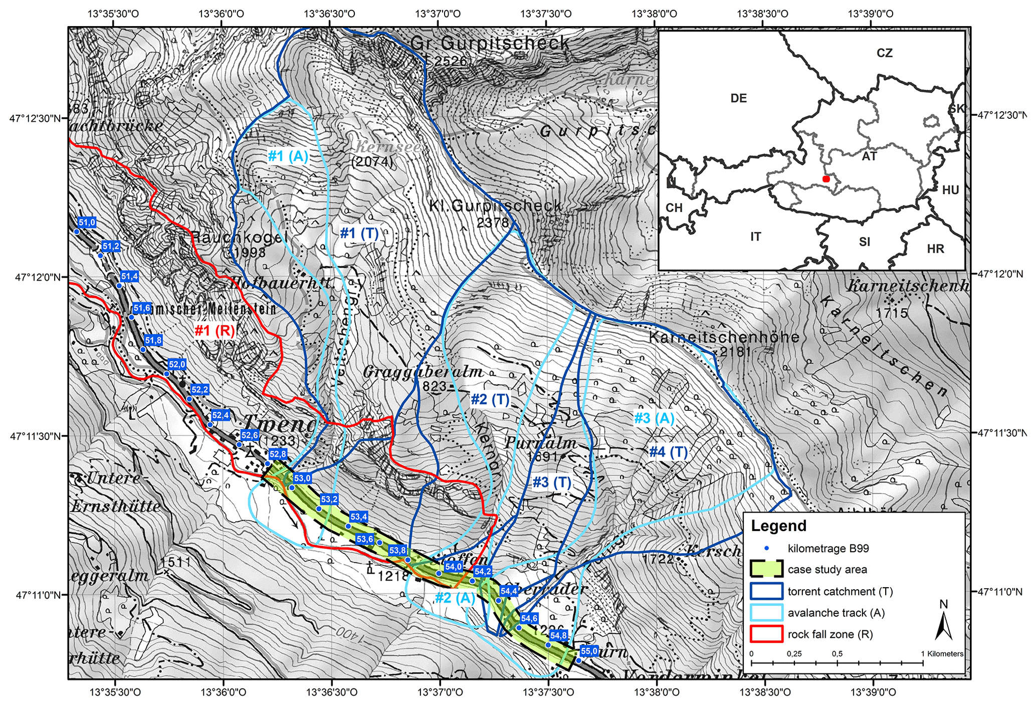
Figure 2Overview of the case study area and location of the natural hazards along the road segment (Source base map: © BEV 2020 – Federal Office of Metrology and Surveying, Austria, with permission N2020/69708).
4.1 Hazard analysis
The hazard analysis was part of technical studies undertaken for the road authority of the federal state of Salzburg (Geoconsult, 2016; Oberndorfer, 2016). The results regarding the spatial impact of the hazard processes on the elements at risk and the corresponding hazard intensities were used for the loss assessment in this research. The hazard assessment included the steps of hazard disposition analysis to detect potential hazard sources within the perimeter of the road followed by a detailed numerical hazard analysis. Therefore, these analyses considered approaches for hazard-specific impact assessment according to the engineering guidelines of e.g. Bründl (2009), ASTRA (2012) and Bründl et al. (2015) and relevant engineering standards and technical regulations (Austrian Standards Organisation, 2009, 2010, 2017). The physical impact parameters of the hazard processes were calculated using numerical simulation software, such as Flow-2D for flash floods and debris flows (Flow-2D Software, 2017), SamosAT (Snow Avalanche MOdelling and Simulation – Advanced Technology) for dense-snow and powder-snow avalanches (Sampl, 2007), and Rockyfor3D for rockfall (Dorren, 2012). The hazard analyses were executed without probabilistic calculations; thus, the generated results were integrated as constant input in the risk analysis.
For the multi-hazard purpose three hazard types were evaluated: (1) hydrological hazards (torrential floods, flash floods and debris flows), (2) geological hazards (rockfall and landslides) and (3) snow avalanches (dense-snow and powder-snow avalanches). For each hazard type, intensity maps for the affected road segment were computed. The intensity maps specify for a specific hazard scenario the spatial extent of a certain physical impact (e.g. pressure, velocity or inundation depth) during a reference period (Bründl et al., 2009). In order to transfer the physical impact to object-specific vulnerability values for further use in the risk assessment, three process-specific intensity classes were distinguished (Table 2). These intensity classes were based on the underlying technical guidelines (Bründl, 2009; ASTRA, 2012; Bründl et al., 2015) and were slightly adapted to comply with the regulatory framework in Austria (Republik Österreich, 1975, 1976; BMLFUW, 2011). Table 2 represents the intensity classes which correspond to the affiliated object-specific vulnerability and lethality values (mean damage values) in Tables A7 and A8.
Table 2Process-specific intensity classes with pressure p, height h (suffix hws refers to water and solids), velocity v, depth d and energy E. These are compiled and adapted from Bründl (2009), ASTRA (2012) and Republik Österreich (1975) in conjunction with Republik Österreich (1976) and BMLFUW (2011). The low intensity class for debris flow has the same intensity indicators as for inundation because it was assumed that low intensity debris flow events have the same characteristics as hydrological processes.
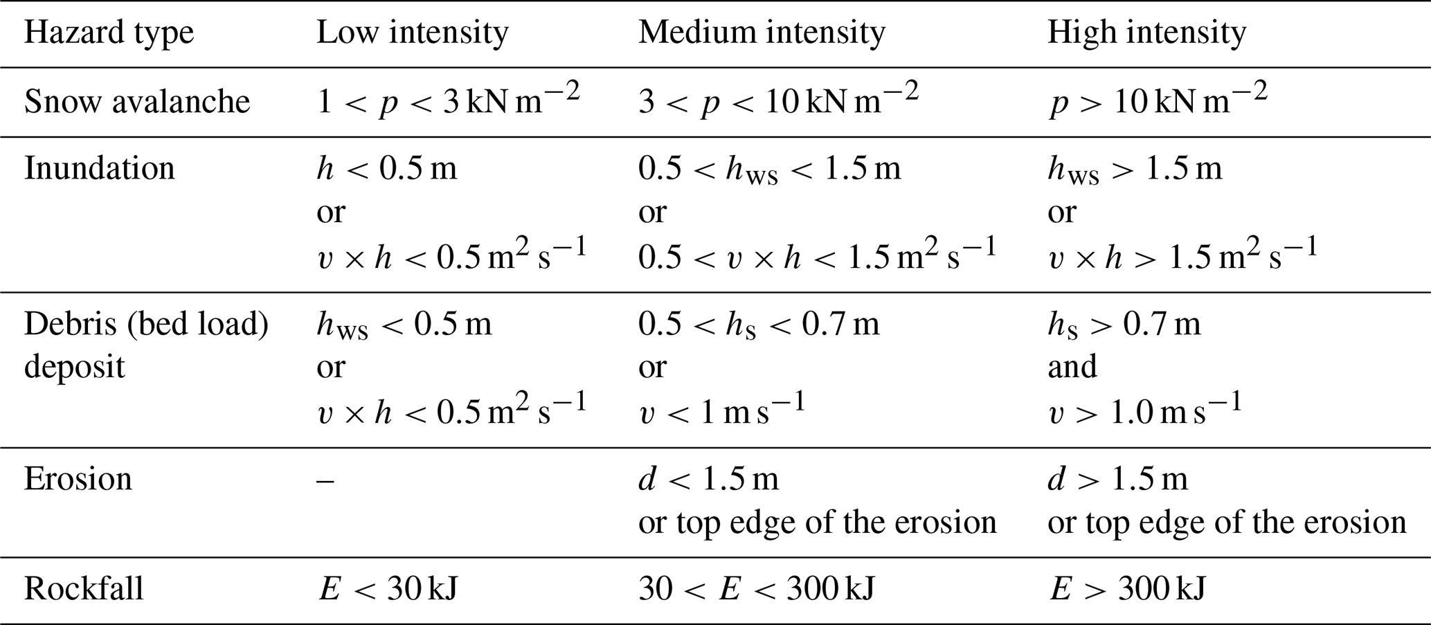
To determine the intensities of individual hazard processes, two different return periods were selected, a 1-in-10-year and a 1-in-30-year event (probability of occurrence p10=0.1 and p30=0.033). All three snow avalanches can either develop as powder-snow avalanches or as dense-snow avalanches, depending on the meteorological and/or snowpack conditions. Due to the catchment characteristics of the torrents two different indicator processes were assigned for assessing the hazard effect, depending on the two occurrence intervals. Therefore, the occurrence interval served as a proxy for the process type, since we assumed for the frequently occurring events (p=0.1) the hazard type “flash floods with sediment transport” and for the medium-scale recurrence intervals (p=0.033) debris flow processes.
4.2 Standard guideline for risk assessment
The method to calculate road risk for our case study followed the deterministic standard framework of the ASTRA (2012) guideline for operational road risk assessment. The identification of elements at risk regarding their quantity, characteristics and value as well as their temporal and spatial variability was assessed through an exposure analysis. The assessment of the vulnerability of objects (affected road segment, culverts, bridges, etc.) and the lethality of persons was carried out by a consequence analysis to characterize the extent of potential losses. The finally resulting collective risk RC (Eq. 2) as a sum of all hazard types over all object classes and scenarios – under the assumption that the occurrence of the individual hazards is independent of each other – was expressed in monetary terms per year as a prognostic value. RC is therefore defined as the expected annual damage caused by certain hazards and is frequently used as a risk indicator (Merz et al., 2009; Špačková et al., 2014). Hence, RC was calculated based on Eq. (1) by summing up the partial risk over all scenarios j and objects i (Bründl et al., 2009, 2015; Bründl, 2009; ASTRA, 2012):
where RC,j is the total collective risk of scenario j and objects i .
According to the ASTRA (2012) guideline, the collective risk RC is divided into three main risk groups: (1) risk for persons RP, (2) property or asset risk RA, and (3) risk of non-operational availability or disposability RD.
4.2.1 Risk for persons RP
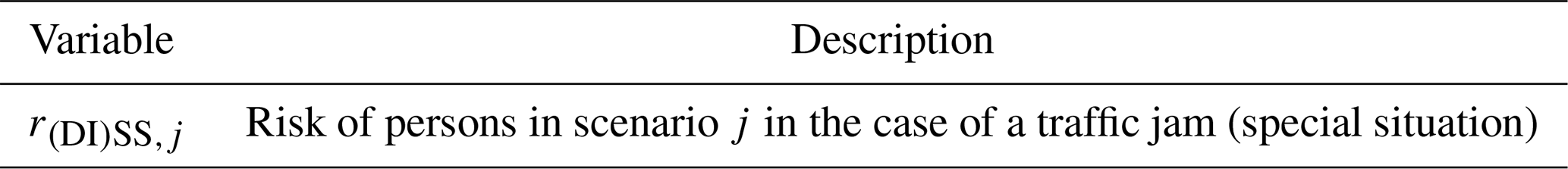
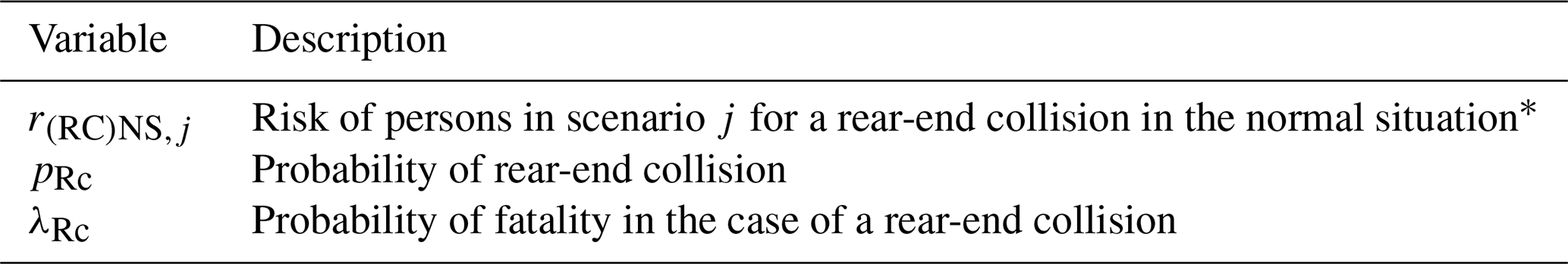
The risk characterization for persons in terms of the direct impact of a natural hazard on cars was distinguished in a standard situation for flowing traffic and a situation during a traffic jam, which was seen as a specific situation leading to a significant increase of potentially endangered persons. Additionally, another specific case was also included representing a rear-end collision either on stagnant cars or on the process depositions on the road in the case of the standard situation. The probability for a rear-end collision depends on the characteristics of the road and is influenced by a factor of e.g. the visual range, the winding and steepness of the road, the velocity, and traffic density (ASTRA, 2012). Furthermore, an additional specific scenario was explicitly considered in the case of the road closure of the main transit route (A10 Tauern motorway) due to the resulting temporal peak of the mean daily traffic. The statistical mean daily traffic (MDT) was used as the mean quantity of persons NP travelling along the road (Table A7).
In order to compute RP, the expected annual losses of persons travelling along the road segment under a defined hazard scenario j was calculated as a combination of the specific damage potential or potential damage extent of persons and the damage probability of the exposure situation k for persons using the road under investigation. The potential losses for persons were monetized by the cost for a statistical human life as published by the Austrian Federal Ministry of Transportation, Innovation and Technology (BMVIT, 2014). The published average national expenses of road accidents include material and immaterial costs (bodily injury, property damage and overhead expenses) of road accidents and are based on statistical evaluations of the national database as well as on the willingness-to-pay approach for human suffering. The monetized costs for a statistical human life equal EUR 3 million. Thus, road risk for persons was calculated with three road-specific exposure situations k (Bründl et al., 2009):
-
direct impact of the hazard event – standard situation (Eq. A1; Table A1),
-
direct impact of the hazard event – specific situation due to a traffic jam (Eq. A2; Table A2),
-
indirect effect – rear-end collision (Eq. A3; Table A3).
The risk variables to assess RP are stated in Table A6 for the exposure situations and in Table A7.
4.2.2 Property risk RA
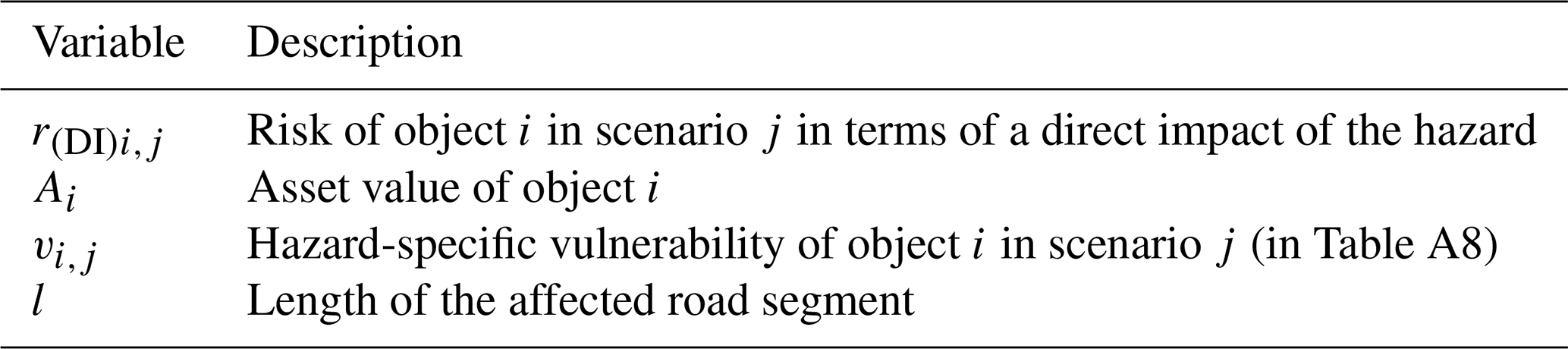
The property risk due to the direct impact of the hazard process on physical assets of the road infrastructure was calculated for each object i and scenario j using Eq. (A4) with Table A4 under consideration of risk variables in Table A8. The damage probability was assumed to be equal to the frequency of the scenario j.
With respect to the potential direct tangible losses within the study area, the physical assets including e.g. the road decking of the street segment, culverts and bridges were expressed by the building costs of the assets calculated from a reference price per unit (Table A8). The physical assets of affected cars were not addressed as this damage type is not included in the standard guideline due to the assumption of obligatory insurance coverage. The monetized costs refer to replacement costs and reconstruction costs, respectively, instead of depreciated values, which is strongly recommended in risk analysis by Merz et al. (2010) due to the fact that replacement cost systematically overestimates the damage. Since there is a limitation of reliable or even available data on replacement costs, the usage of reconstruction costs is a pragmatic procedure to calculate damage.
4.2.3 Risk due to non-operational availability RD
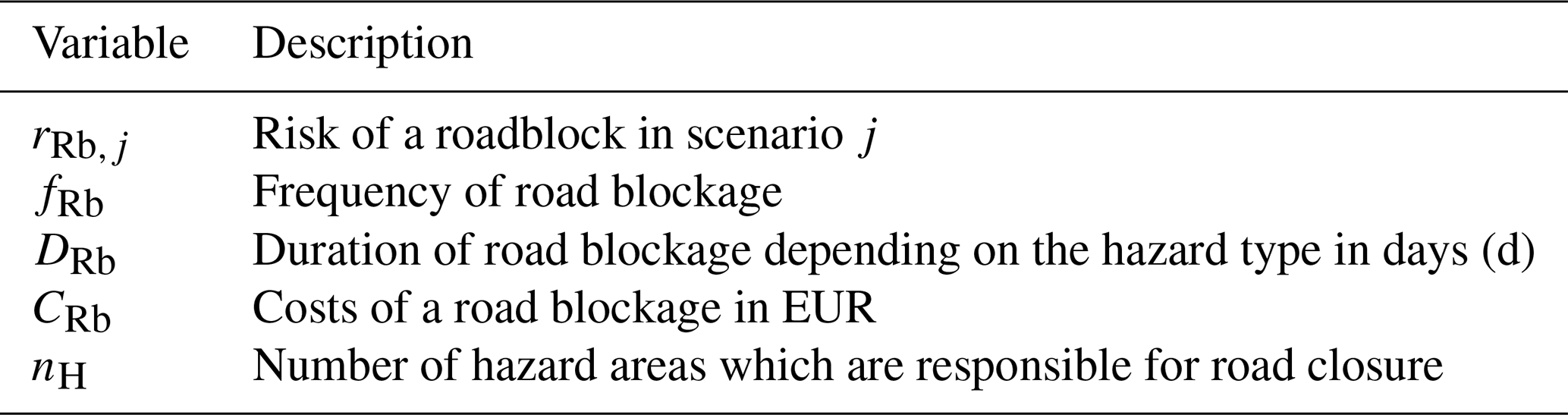
The risk due to non-operational availability can be generally separated into economic losses due to (1) road closure after a hazard event or (2) as a result of precautionary measures for road blockage. The former addresses the mandatory reconditioning of the road, and interruption time depends on the severity of the damage. For our case study, only the precautionary non-operational availability was calculated with Eq. (A5), Table A5 and variables in Table A9 because the village of Obertauern can be accessed from both directions of the mountain pass road. Therefore, a general accessibility of the village was supposed because it was assumed that events only lead to a road closure on one side of the pass. Potential costs resulting from time delays for necessary detours or e.g. from an increase of environmental or other stresses were neglected. The maximum intensity of the process served as a proxy for the duration of the road closure.
The direct intangible costs for non-operational availability of the road were approximated from statistical data accounting for the business interruption and the loss of profits of the tourism sector in the village of Obertauern due to road closure (see Table A9). The village of Obertauern is a major regional tourism hot spot, and therefore the predominant income revenues are based on tourism; thus other business divisions were neglected. Regarding the precautionary expected losses only snow avalanches were included, due to the obligatory legal implementation of monitoring by a regional avalanche commission. Thus, a reliable procedure for a road closure could be assumed.
4.3 Risk computation
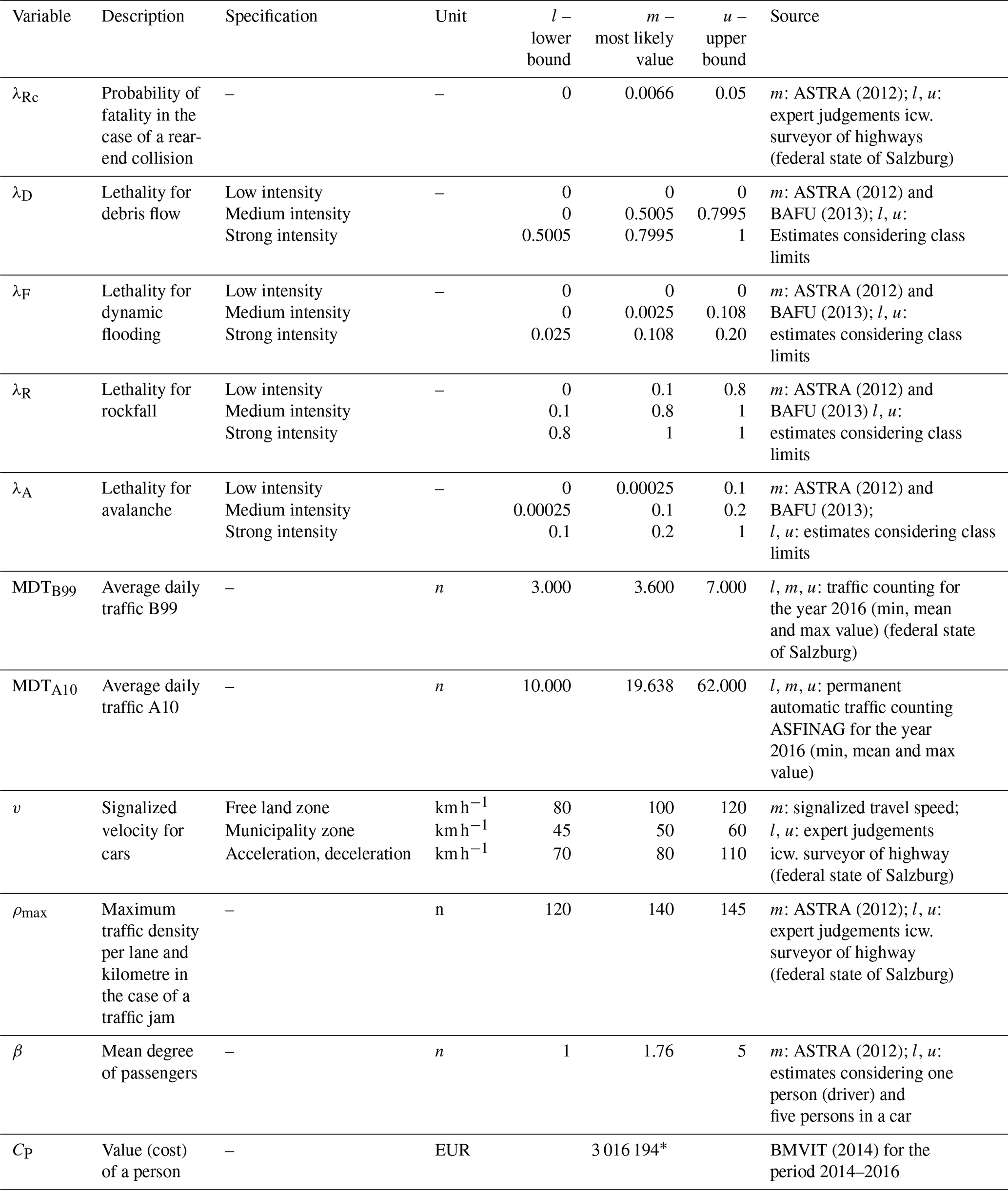
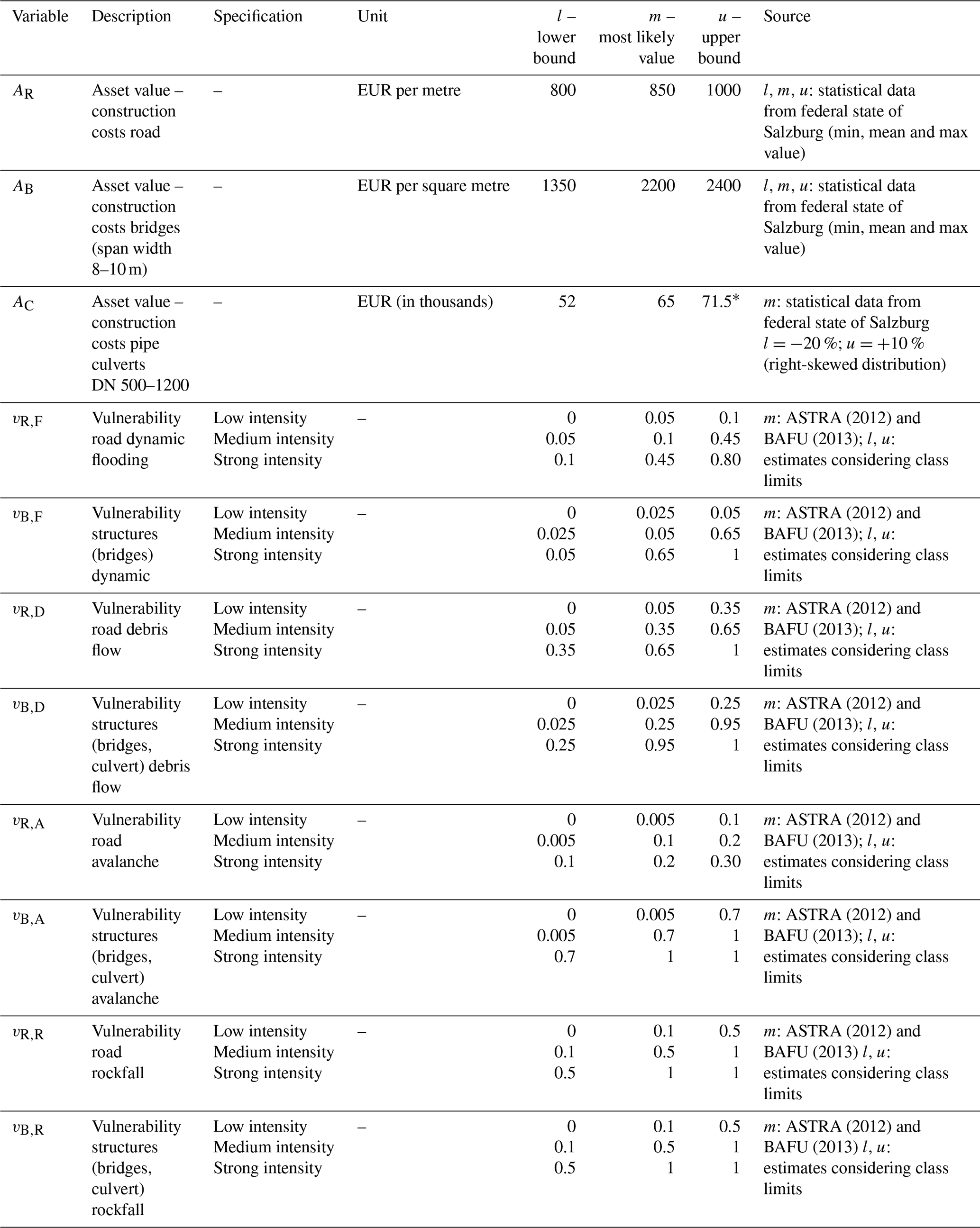
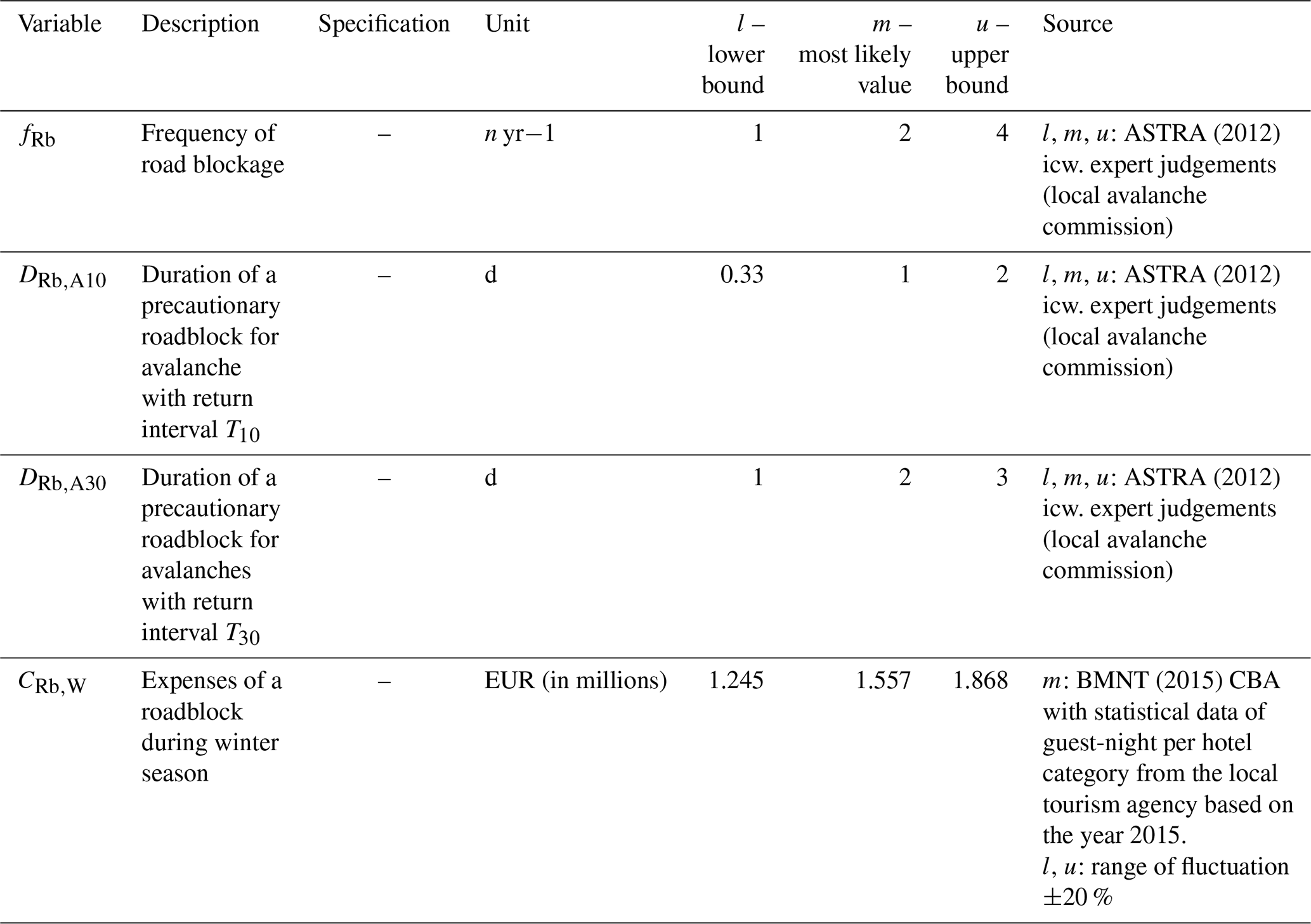
For the purpose of computing road risk, the risk Eqs. (A1) to (A5) from the standard guideline (ASTRA, 2012), stated in the Appendix in conjunction with Tables A1 to A5, were used without further modification both for the deterministic and for the probabilistic calculation. Hence, the probabilistic setup is based on the same equations as the standard approach, but the variables were addressed with probability distributions instead of single values. In a first step, the deterministic result was computed as a base value for comparison with the results (probability density functions, PDFs) of the two diverging probabilistic setups. In a second step, a probabilistic model was integrated into the same calculation setup to consider the bandwidth of the risk-contributing variables. Using this probabilistic model, the individual risk variables were addressed with two separate probability distributions. The flowchart in Fig. 1 illustrates the risk assessment method and distinguishes between the deterministic and the probabilistic risk model. The diagram exemplarily demonstrates the calculation steps for both model setups. Whereas only the single value of the input data was processed within the standard (deterministic) setup, the probabilistic risk model utilized the bandwidth of each variable denoted in Tables A6 to A9. These values were either defined from statistical data, expert judgement or existing literature. The range represents the assumed potential scatter of the variables including a minimum (lower bound l), an expected or most likely value (m) and a maximum value (upper bund u). The deterministic setup was calculated with the expected value, which corresponds in most cases to the recommended input value of the guideline. The choice of the variable range in Tables A6 to A9 is case study specific and cannot be transferred to other studies without careful validation.
4.3.1 Probabilistic framework
Within the probabilistic risk modelling setup, the contributing variables for computing the prognostic annual loss were calculated in a stochastic way using their potential range. The probabilistic risk calculation was conducted with the software package RIAAT – Risk Administration and Analysis Tool (RiskConsult GmbH, 2015). The probabilistic setup comprised two different and independent calculation runs each with two different distribution functions to characterize the uncertainty of the input variables. Hence, each variable was modelled using either (1) a triangular or three-point distribution (TPD) or (2) a beta-PERT (programme evaluation and review technique) distribution (BPD) within the probabilistic model, which generated two independent probabilistic setups and results. The discrete risk calculation with two different approaches of probability distributions facilitated a comparison of the applicability and the sensitivity of the simple distribution functions on the results. The expected annual monetary losses induced by the three hazard types were aggregated and further compacted to the probability density function (PDF) of the total risk caused by multi-hazard impact. Finally, the two different PDFs from the stochastic risk assessment were compared with the result from the deterministic method to show the potential dynamics in the results.
Triangular distribution (TPD)
The triangular distribution derives its statistical properties from the geometry: it is defined by three parameters l for the lower bound, m for the most likely value (the mode) and u for the upper bound. Whereas lower and upper bounds define on both edges the limited bandwidth, the most likely value indicates that values in the middle are more probable than the boundary values and also allows for the representation of skewness. The TPD is a popular distribution in the risk analysis field (Cottin and Döhler, 2013) for example to reproduce expert estimates. Especially if little or no information about the actual distribution of the parameter or only an estimate of the additional variables to fit the theoretical distribution is feasible, a best possible approximation can be achieved using the TPD. If there is no representative empirical data available as a basis for risk prediction, complex analytical (theoretical) distributions, which are harder to model and communicate, may not represent the reality better than a simple triangular distribution (Sander, 2012).
Beta-PERT distribution (BPD)
The beta-PERT distribution (programme evaluation and review technique) is a simplification of the beta distribution with the advantage of an easier modelling and application (Sander, 2012). It requires the same three parameters as a triangular distribution: l for the lower bound, m for the most likely value (mode) and u for the upper bound. In contrast to the two parametric normal distribution N(μ, σ) – μ for average and σ for standard deviation – the beta-PERT distribution is limited on the edges and allows for modelling asymmetric situations. Risk parameters commonly have a natural boundary, for example vulnerability factors ranging from 0 (no loss) to 1 (total loss). Therefore, estimating min–max values instead of standard deviation is more realistic or feasible, as there are in most cases no data available to express the mean variation. Moreover, BPD allows for smoother shapes, making it suitable to model a distribution that is actually an aggregation of several other distributions.
For a given number of risks, each with a probability of occurrence and an individual probability distribution, the potential number of combinations (scenarios) escalates nonlinearly. Especially if dependencies or correlations between different risks are included and/or numerous partial risks are aggregated to an overall risk the application of analytical methods have computational restrictions. Stochastic simulations are better suited to work on such complex models (Tecklenburg, 2003). Therefore, the aggregation of the distributions were calculated by means of Latin hypercube sampling (LHS), which is a stochastic simulation technique comparable to Monte Carlo simulation (MCS) with the advantages of faster data processing, better fitting on the theoretical input distribution and more efficient calculation, as fewer iterations are needed to get equally good results (Sander, 2012). LHS consistently produces values for the distribution's statistics that are nearer to the theoretical values of the input distribution than MCS. These advantages are possible because the real random numbers used to select samples for the MCS tend to have local clusters, which are only averaged out for a very large number of draws. Addressing this issue using LHS can immediately improve the quality of the result by splitting the probability distribution into n intervals of equal probability, where n is the number of iterations that are to be performed on the model. In the present study, 1 000 000 iterations where performed for every single simulation to get consistent results.
In Table 3 the results for each risk group (RP, RA and RD) as well as for the total multi-hazard risk RC calculated with the standard deterministic risk approach are shown and compared to those obtained by the two probabilistic setups using two different probability distributions (TPD and BPD). The results associated with the two distribution functions are displayed as a median value of the PDF to show their deviation to the outcome of the standard approach. Based on our case study, the road risk over all hazard types and scenarios (multi-hazard risk) with the deterministic approach results in EUR 76.0 thousand per year. The results with the probabilistic approach referring to the median of the PDFs amounts to a monetary risk of EUR 105.6 thousand per year (TPD) and EUR 90.9 thousand per year (BPD), respectively. Compared to the standard approach the median of the PDFs equals an increase of 38 % (BPD) and 19 % (TPD), depending on the choice of probability distribution to model the uncertainties of the input variables. Focusing on the 95th percentile (P95) of the results – non-exceedance probability of 95 %, shown in Fig. 3 – an increase of 79 % (TPD) and 46 % (BPD) to the deterministic result can be observed. Figure 3 illustrates, based on the Lorenz curves for the two distributions (TPD and BPD), the scale of deviation of the total multi-hazard risk RC within the probabilistic risk modelling and compared to the standard outcome. The graphs show the potential uncertainties of the risk computation, which can be covered by a suitable choice of a value-at-risk (VaR) level. For example, with a benchmark of the 95th percentile (P95), 95 % of the potential uncertainties within the risk calculation can be covered by using a probabilistic risk assessment approach. However, a suitable VaR level depends on the general safety requirement of the system as well as on the degree of uncertainty of the input variables.
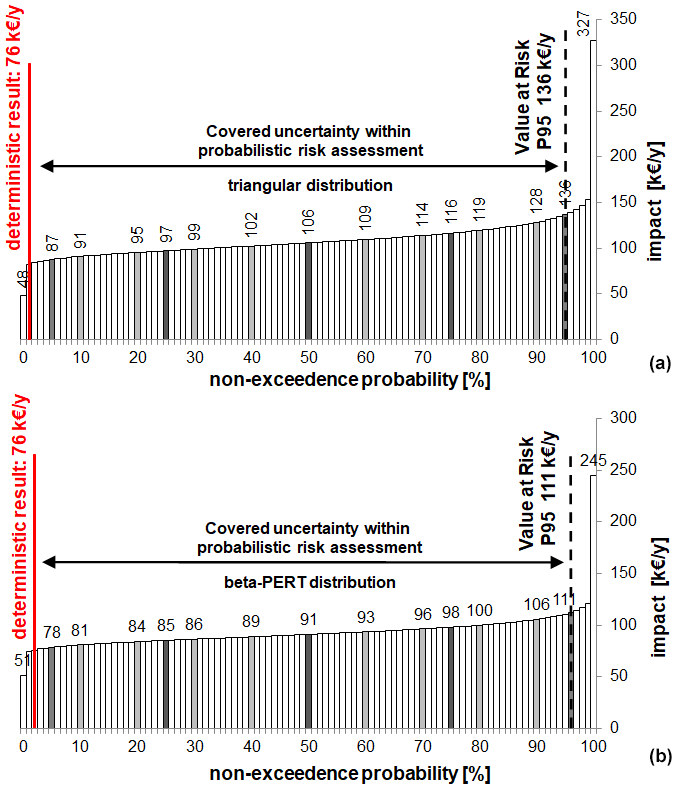
Figure 3Lorenz curves for a (a) triangular distribution and (b) beta-PERT distribution showing the scale of deviation of the total multi-hazard risk RC within the probabilistic risk modelling and compared to the deterministic result (in units of thousands of EUR per year).
Geological hazards (rockfall) contribute with a fraction of 7.8 % to the total risk (or, in absolute numbers, EUR 5.9 thousand, see Table 3) based on the deterministic model, which can be attributed to the relatively small importance in comparison to the other hazard types in the study area. Hydrological hazards pose the highest risk (50.5 %, or, in absolute numbers, EUR 38.4 thousand per year) previous to avalanche hazards (41.7 %, or, in absolute numbers, EUR 31.7 thousand per year). Overall, RP (44.9 %; EUR 34.1 thousand per year) has the highest share on the total multi-hazard risk narrowly followed by RA (38.9 %; EUR 29.6 thousand per year), both associated with direct damage. The hydrological hazards (predominantly debris flow processes) with a portion of 76.5 % or EUR 26.1 thousand per year have a disproportionately high share on RP due to the high-intensity hazard impact. Similarly, the semi-empirical lethality factors shown in Table A7 have high values (λD=0.8) just like the impact of rockfall on cars with a probability of death of λR=1.0. Thus, these event types yield in high monetary losses in contrast to snow avalanches with a lethality factor for a high intensity of λA=0.2. By modelling the hazard-specific lethality with probability functions a wider scatter can be achieved, but the effect still remains due to the heavy weight around the most likely value m. The indirect losses related to RD with a fraction of 16.3 %, or, in absolute numbers, EUR 12.4 thousand per year have a minor portion because this risk group is only relevant for snow avalanches.
Table 3Comparison of the deterministic versus probabilistic results for the three risk categories depending on the three hazard types and the total collective risk with risk for persons RP, asset risk RA, disposability risk RD and total collective risk RC with absolute values (in units of thousands of EUR per year) in the first row and as percentage in the second row. For the probabilistic data, the median value of the triangular or three-point distribution (TPD) and the beta-PERT distribution (BPD) functions are displayed. Note that risk-based aggregated losses do not equal the sum of the sub-components because probabilistic metrics such as P50 are not additive. Thus, the computational sum as well as the percentage are slightly different.

The results related to our case study (Table 3 and Fig. 4) show that due to the shape and the mathematical definition of the distribution the TPD leads to the highest variation in the monetary losses. The boxplots in Fig. 4 display the results from the probabilistic simulation for the three risk categories (RP, RA and RD) and for the total hazard-specific risk (RC) relating to the three hazard types (Fig. 3a–c) and for the total multi-hazard collective risk (Fig. 4d) with respect to the measures of the central tendency of the PDF. The boxplot diagrams are thereby plotted against the deterministic value to show its position. The wide range of the distribution in RC is markedly caused by RP, which exhibits a broad bandwidth and a right-skewed distribution. Hence, unlike RA and RD, the physical injuries expressed as the economic losses of persons (RP) are responsible for the highest divergence to the standard approach and show a considerable scatter. The main causes for the striking deviations can be associated with the relatively high monetary value of persons which was modelled as discrete point value in combination with the fluctuations of the MDT and the variations of the hazard-specific lethality. The monetized costs for a statistical human life equal EUR 3 million (Table A7) and are based on a statistical survey of the economic expenses for a road accident in Austria (BMVIT, 2014). Although we ascribe this value to a high degree of uncertainty the valuation of the expenses for a statistical human life was not attributed to a probability distribution due to the case-study-specific fixed governmental requirements in Austria. The discussion of a monetarily evaluation of a human life is still ongoing across scientific disciplines using different economic approaches (e.g. Hood, 2017). Furthermore, the lethality factors also correspond to the high variation of RP which are seen as very sensitive parameters. Therefore, we encourage further research on hazard-specific lethality functions for road risk management either based on comprehensive empirical datasets or on representative hazard impact modelling. Due to the strong effect of RP on RC the results have to be carefully interpreted, as they are sensitive to the input variables. Therefore, the values in our case study especially the cost for human life cannot be directly transferred to other application without a detailed validation and verification of national regulations.

Figure 4Probabilistic results for the three risk categories per hazard type (a torrent processes, b snow avalanches and c rockfall) and for the total collective risk (d) based on the two distribution functions triangular or three-point distribution (TPD) and the beta-PERT distribution (BPD) with risk for persons RP, asset risk RA, disposability risk RD and total collective risk RC (in units of thousands of EUR per year).
Apart from RP where the deterministic result is located below or near the 5th percentile of both PDFs, RA and RD are mostly within the interquartile range between the 25th quartile and the median compared to the standard approach (Fig. 4). In this context, RA for snow avalanche exceeds the median and is situated between the median and the 75th quartile. The effect can be traced back to the left-skewed distribution of the vulnerability factor vB,A for medium avalanche hazard intensities regarding the object class structures (bridges and culverts) in Table A8. In general, due to the shape and the mathematical characteristics of the distribution, the BPD leads to a stronger compaction around the median than the TPD which can be well explained by the properties of the BPD which has, in comparison to the TPD, a larger weight around the most likely value m.
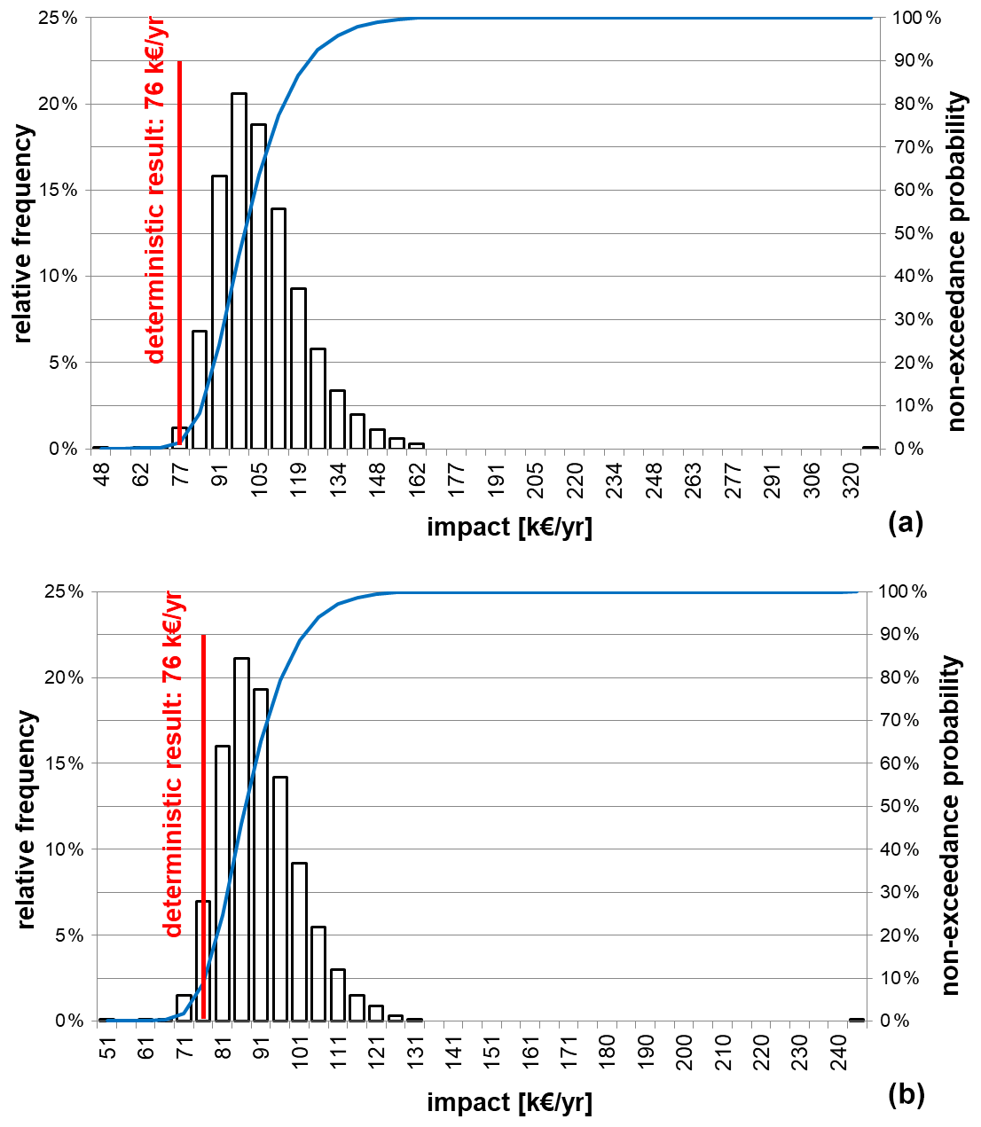
Figure 5Probability density function (PDF) and cumulative distribution function (CDF) for a (a) triangular distribution and (b) beta-PERT distribution (in units of thousands of EUR per year).
In Fig. 5, the PDF and the cumulative distribution function (CDF) are shown for RC with the two probabilistic model results and the deterministic result. In both cases (TPD and BPD), the deterministic result is situated at the lower edge of the PDF near or under the 5th percentile. Thus, the deterministic result of our case study covers approximately less than 5 % of the potential bandwidth of the probability distribution. The TPD has a wide range, whereas the BPD is considerably flattened on the boundary of the amplitude. The results of the two distributions have in common that they are allocated right skewed. In contrast to the location of the median, the deterministic result is on the far-left side of both distributions and is exceeded by more than 95 % of the potential outcome.
The results based on our case study provide evidence that the monetary risk calculated with a standard deterministic method following the conventional guidelines is lower than applying a probabilistic approach. Thus, without consideration of uncertainty of the input variables risk might be underestimated using the operational standard risk assessment approach for road infrastructure. The mathematical product of the frequency of occurrence and the potential consequences with single values and, in a narrower sense, the multiplication of the partial risk factors in the second part of the risk equation may lead to a bias in the risk magnitude because the multiplication of the ancillary calculations generates a theoretical value ignoring the full scope of the total risk.
The far-left position of the deterministic value within the PDF of the probabilistic result in our study can be traced back to fact that the multiplication of two positive symmetrical distributions results in a right-skewed distribution because the product of the small numbers at the lower ends of the bandwidths results in much smaller numbers than the product of the high numbers at the upper ends of the bandwidths. When right-skewed distributions are used as an input and aggregated, the effect of skewness shifts the deterministic value (represented by the most likely value) to the left side of the resulting distribution. Even if conservative risk values are used in a deterministic setup, a potential scatter (upper and lower bounds) remains, which leads within a probabilistic calculation through aggregation of the partial risk elements and sub-results to a right-skewed distribution according to the skewness of input variables. Since risk values of our study are in most cases asymmetric with primarily positive skews, the deterministic result migrates during aggregation to the left side of the PDF in Fig. 5. The deterministic risk value is usually expressed either as a theoretical mean value or as the most likely value, neglecting the potential distribution functions of the input data. Thus, the compression of the input values to a single deterministic risk value with total determination prevents an actual prognosis of reliability that would have been achieved by specifying bandwidths (Sander, 2012). Furthermore, the simple summation of the scenario related and the object-based risk to receive the cumulative risk level instead of using probabilistic risk aggregation leads to an underestimation of the final risk. Hence, the full spectrum of risk cannot be represented with deterministic risk assessment, which may further lead to biased decisions on risk mitigation.
The value-at-risk (VaR) approach by considering a reliable percentile of the non-exceedance probability e.g. P95 as shown in Fig. 3 – depending on the desired coverage of the risk potential from society, authorities or organizations – might be an appropriate concept to tackle this challenge. In this context, a higher VaR value implies a higher safety level for the system under investigation. The final results of risk assessments are subject to uncertainties mainly due to insufficient data basis of input variables, which can be addressed using a PDF to represent uncertainties involved. For further decisions on the realization of mitigation measures a high VaR value such as P95 covers these uncertainties with a defined shortfall probability and thus supports decision-makers with more information about road risk. In turn, as a further practical improvement this benchmark can be compared to the same grade of safety for the costs of mitigation measures, since cost assessments for defence structures are also subject to considerable uncertainties. Thus, an optimal risk-based design of defence structures might encompass a balance between the same VaR level both of a probabilistic risk and a probabilistic cost assessment utilizing a cost–benefit analysis (CBA). However, within a probabilistic approach the scale of deviation is dependent on the choice of distribution for modelling the bandwidth of the variables, and the results are sensitive to the defined spectrum of input information stated in Tables A6–A9. These variables are case study specific and cannot be directly transferred to other road risk assessments without careful validation. However, probabilistic risk assessment (PRA) enables a transparent representation of potential losses due to the explicit consideration of the entire potential bandwidth of the variables contributing to risk. Since comparable results can be achieved based on predefined values (Bründl et al., 2009), we still recommend the consideration of the deterministic value as a comparative value to the probabilistic method.
Road risk assessment is usually afflicted with data scarcity; thus, risk operators and practitioners are often dependent on expert appraisals, which are subject to uncertainties. In order to improve data quality, upper and lower values and the expected value can be easily estimated for fitting a simple distribution of the input variables. Even though empirical values such as statistical data are available, a certain degree of uncertainty remains. Therefore, simple distribution functions such as TPD or BPD can adjust the shape of the distribution more conveniently than complex probability distributions, since the required additional parameters to adjust a complex distribution are simple not available. Hence, for a prognostic prediction, risk modelling with complex distributions in contrast to simple techniques cannot be justified if there is a lack of empirical data.
A limitation of our study is that the performance of the probabilistic approach cannot be verified and validated with empirical data, but the results show that the explicit inclusion of epistemic uncertainty leads to a bias in risk magnitude. The probabilistic approach allows for the quantification of uncertainty and thus enables decision-makers to better assess the quality and validity of the results from road risk assessments. This can facilitate the improvement of road safety guidelines (for example by implementing a VaR concept) and thus is of particular importance for authorities responsible for operational road safety, for design engineers and for policymakers due to a general increase of information for optimal decision-making under budget constraints. Furthermore, the paper addresses the second part of the risk concept in terms of the consequence analysis. The results of the hazard analysis serve thereby as a constant input using the physical modelling of the hazard processes without the consideration of probabilistic methods. Thus, the probability of occurrence of the hazard processes was mathematically processed as a point value within the probabilistic design, since the hazard analyses (with deterministic design events to assess the hazard intensities as a function of the return interval) was part of prior technical studies. Further considerations of a probabilistic modelling of the frequency of the events were outside of the study design and might be addressed in subsequent studies. Therefore, we expect a considerable source of epistemic uncertainty within the hazard analysis which emphasizes the necessity for the additional inclusion of probability-based hazard analyses in a holistic multi-hazard risk environment. Even though the presented methodology in this study focuses on a road segment exposed to a multi-hazard environment on a local scale, the approach can easily be transferred to other risk-oriented purposes.
A1 Risk for persons RP
A1.1 Direct impact of the hazard event – standard situation
Table A1Risk variables and their derivation for the calculation of RP: direct impact – standard situation. 1 The reduction factor considers that not all hazard areas get simultaneously released by the same triggering event. 2 The number of hazard areas for the three hazard types was calculated as discrete values based on field surveys according to the release probability as a function of the event frequency (avalanches: nA10=6, nA30=7; torrent processes: nT10=7, nT30=8; rockfall: pRbE=0, not relevant). 3 The length of the affected street segment is a discrete (single) value according to the results of the hazard analyses.

A1.2 Direct impact of the hazard event – special situation due to a traffic jam
Table A2Risk of persons in scenario j for the calculation of RP: direct impact – traffic jam. The calculation of the variables is according to Table A1.
A1.3 Indirect effect – rear-end collision
Table A3Risk variables and their description for the calculation of RP: rear-end collision. The calculation of the residual variables is according to Table A1. * A rear-end collision is only valid in the case of a standard situation (no traffic jam). The scenario is not relevant for low-intensity hazard events with deposition heights < 0.15 m.
A2 Property risk RA
Table A4Risk variables and their description for the calculation of RA: direct impact. The calculation of the residual variables is according to Table A1.
A3 Risk due to non-operational availability RD
Table A5Risk variables and their description for the calculation of RD. The calculation of the residual variables is according to Table A1.
Risk variables
A4 Probability of loss – exposure
Table A6Bandwidth (credible intervals with l – lower bound, m – most likely value and u – upper bound) of the variables within the probabilistic risk analysis for calculating exposure situations. Units: h for hours, n for numbers and yr for years. ASFINAG: Autobahnen- und Schnellstraßen-Finanzierungs-Aktiengesellschaft; in consultation with: icw. * Event types 1, 5 and 10 equate to single-stone, multiple-stone and small-scale rockslide, respectively.

A5 Degree of damage – risk for persons RP
Table A7Bandwidth (credible intervals with l – lower bound, m – most likely value and u – upper bound) of the variables within the probabilistic risk analysis for calculating RP. Units: h for hours and n for numbers. * The monetary value of a person was used as single (point) value, as this value is recommended by the Austrian government.
A6 Extent of damage – risk for material assets RA
Table A8Bandwidth (credible intervals with l – lower bound, m – most likely value and u – upper bound) of the variables within the probabilistic risk analysis for calculating RA. * Base value according to the federal state of Salzburg: %, % (right-skewed distribution). DN: nominal diameter.
A7 Degree of damage – risk for operational availability RD
Table A9Bandwidth (credible intervals with l – lower bound, m – most likely value and u – upper bound) of the variables within the probabilistic risk analysis for calculating RD. Units: d for days, n for numbers and yr for years.
All risk-related data are publicly available (see references throughout the paper as well as in the Appendix).
SO initiated the research; was responsible for data collection, literature research, the preparation of the paper and the visualization of the results; and performed the risk simulations with additional contributions by PS. PS contributed to additional information on probabilistic risk calculation. SF compiled the background on risk assessment and helped to shape the research, analysis and the paper. All authors discussed the results and contributed to the final paper.
Sven Fuchs is member of the Editorial Board of Natural Hazards and Earth System Sciences.
This work was supported by the government of the federal state of Salzburg, Austria, especially from the Geological Survey under supervision of Ludwig Fegerl and Gerald Valentin. The geological hazard analysis was conducted by Geoconsult ZT GmbH by Andreas Schober on behalf of the government of the federal state of Salzburg, which provided the hazard data for the risk analysis.
Open-access funding was provided by the BOKU Vienna (University of Natural Resources and Life Sciences, Vienna) Open Access Publishing Fund.
This paper was edited by Thomas Glade and reviewed by two anonymous referees.
Apel, H., Thieken, A. H., Merz, B., and Blöschl, G.: Flood risk assessment and associated uncertainty, Nat. Hazards Earth Syst. Sci., 4, 295–308, https://doi.org/10.5194/nhess-4-295-2004, 2004.
ASTRA: Naturgefahren auf Nationalstraßen: Risikokonzept, Methodik für eine risikobasierende Beurteilung, Prävention und Bewältigung von gravitativen Naturgefahren auf Nationalstraßen V2.10, Bundesamt für Straßen (ASTRA), Bern, Switzerland, 98 pp., 2012.
Austrian Standards International: Protection works for torrent control – Terms and their definitions as well as classification, ONR 24800:2009 02 15, Austrian Standards International, Vienna, 2009.
Austrian Standards International: Permanent technical avalanche protection – Terms, definition, static and dynamic load assumptions, ONR 24805:2010 06 01, Austrian Standards International, Vienna, 2010.
Austrian Standards International: Technical protection against rockfall – Terms and definitions, effects of actions, design, monitoring and maintenance, ONR 24810:2017 02 15, Austrian Standards International, Vienna, 2017.
BAFU – Bundesamt für Umwelt BAFU: Objektparameterliste EconoMe 2.2, Bern, 2013.
Bell, R. and Glade, T.: Quantitative risk analysis for landslides – Examples from Bíldudalur, NW-Iceland, Nat. Hazards Earth Syst. Sci., 4, 117–131, https://doi.org/10.5194/nhess-4-117-2004, 2004.
Benn, J. L.: Landslide events on the West Coast, South Island, 1867–2002, New Zeal. Geogr., 61, 3–13, https://doi.org/10.1111/j.1745-7939.2005.00001.x, 2005.
BMLFUW: Richtlinie für Gefahrenzonenplanung, available at: https://www.bmlrt.gv.at/forst/wildbachlawinenverbauung/richtliniensammlung/GZP.html (last access: 23 November 2020), 2011.
BMNT: Richtlinien für die Wirtschaftlichkeitsuntersuchung und Priorisierung von Maßnahmen der Wildbach- und Lawinenverbauung (Kosten-Nutzen-Untersuchung), available at: https://www.bmnt.gv.at/forst/wildbach-lawinenverbauung/richtliniensammlung/Richtlinien.html (last access: 1 June 2016), 2015.
BMVIT: Durchschnittliche Unfallkosten Preisstand 2011, Bundesministerium für Verkehr, Innovation und Technologie BMVIT, available at: https://www.bmvit.gv.at/verkehr/strasse/sicherheit/strassenverkehrsunfaelle/ukr2012.html (last access: 1 June 2016), 2014.
Bründl, M. (Ed.): Risikokonzept für Naturgefahren-Leitfaden, Nationale Plattform für Naturgefahren (PLANAT), Bern, Switzerland, 422 pp., 2009.
Bründl, M., Romang, H. E., Bischof, N., and Rheinberger, C. M.: The risk concept and its application in natural hazard risk management in Switzerland, Nat. Hazards Earth Syst. Sci., 9, 801–813, https://doi.org/10.5194/nhess-9-801-2009, 2009.
Bründl, M., Bartelt, P., Schweizer, J., Keiler, M., and Glade, T.: Review and future challenges in snow avalanche risk analysis, in: Geomorphological Hazards and Disaster Prevention, edited by: Alcántara-Ayala, I. and Goudie, A. S., Cambridge University Press, Cambridge, UK, 49–61, 2010.
Bründl, M., Ettlin, L., Burkard, A., Oggier, N., Dolf, F., and Gutwein, P.: EconoMe – Wirksamkeit und Wirtschaftlichkeit von Schutzmaßnahmen gegen Naturgefahren, Formelsammlung, available at: https://econome.ch/eco_work/doc/Formelsammlung_EconoMe_4-0_2016_D.pdf (last access: 23 November 2020), 2015.
Bunce, C., Cruden, D., and Morgenstern, N.: Assessment of the hazard from rock fall on a highway, Can. Geotech. J., 34, 344–356, https://doi.org/10.1139/t97-009, 1997.
Ciurean, R. L., Hussin, H., van Westen, C. J., Jaboyedoff, M., Nicolet, P., Chen, L., Frigerio, S., and Glade, T.: Multi-scale debris flow vulnerability assessment and direct loss estimation of buildings in the Eastern Italian Alps, Nat. Hazards, 85, 929–957, https://doi.org/10.1007/s11069-016-2612-6, 2017.
Cottin, C. and Döhler, S.: Risikoanalyse. Modellierung, Beurteilung und Management von Risiken mit Praxisbeispielen, Springer Spektrum, Wiesbaden, Germany, https://doi.org/10.1007/978-3-658-00830-7, 2013.
Dai, E. C., Lee, C. F., and Ngai, Y. Y.: Landslide risk assessment and management: an overview, Eng. Geol., 64, 65–87, https://doi.org/10.1016/S0013-7952(01)00093-X, 2002.
Dorren, L. K. A.: Rockyfor3D (V5.1) Transparent description of the complete 3D rockfall model, available at: https://www.ecorisq.com (last access: 1 June 2016), 2012.
Fell, R., Corominas, J., Bonnard, C., Cascini, L., Leroi, E., and Savage, W.: Guidelines for landslide susceptibility, hazard and risk zoning for land-use planning, Eng. Geol., 102, 85–98, https://doi.org/10.1016/j.enggeo.2008.03.022, 2008a.
Fell, R., Corominas, J., Bonnard, C., Cascini, L., Leroi, E., and Savage, W.: Guidelines for landslide susceptibility, hazard and risk zoning for land-use planning – Commentary, Eng. Geol., 102, 99–111, https://doi.org/10.1016/j.enggeo.2008.03.014, 2008b.
Ferlisi, S., Cascini, L., Corominas, J., and Matano, F.: Rockfall risk assessment to persons travelling in vehicles along a road: the case study of the Amalfi coastal road (southern Italy), Nat. Hazards, 62, 691–721, https://doi.org/10.1111/nzg.12170, 2012.
Flow-2D Software: Flow-2D Reference Manual, Flow-2D Software Inc., Nutrioso, 2017.
Fuchs, S.: Susceptibility versus resilience to mountain hazards in Austria – paradigms of vulnerability revisited, Nat. Hazards Earth Syst. Sci., 9, 337–352, https://doi.org/10.5194/nhess-9-337-2009, 2009.
Fuchs, S., Heiss, K., and Hübl, J.: Towards an empirical vulnerability function for use in debris flow risk assessment, Nat. Hazards Earth Syst. Sci., 7, 495–506, https://doi.org/10.5194/nhess-7-495-2007, 2007.
Fuchs, S., Keiler, M., Sokratov, S., and Shnyparkov, A.: Spatiotemporal dynamics: the need for an innovative approach in mountain hazard risk management, Nat. Hazards, 68, 1217–1241, https://doi.org/10.1007/s11069-012-0508-7, 2013.
Fuchs, S., Keiler, M., and Zischg, A.: A spatiotemporal multi-hazard exposure assessment based on property data, Nat. Hazards Earth Syst. Sci., 15, 2127–2142, https://doi.org/10.5194/nhess-15-2127-2015, 2015.
Fuchs, S., Röthlisberger, V., Thaler, T., Zischg, A., and Keiler, M.: Natural hazard management from a coevolutionary perspective: Exposure and policy response in the European Alps, Ann. Am. Assoc. Geogr., 107, 382–392, https://doi.org/10.1080/24694452.2016.1235494, 2017.
Fuchs, S., Keiler, M., Ortlepp, R., Schinke, R., and Papathoma-Köhle, M.: Recent advances in vulnerability assessment for the built environment exposed to torrential hazards: Challenges and the way forward, J. Hydrol., 575, 587–595, https://doi.org/10.1016/j.jhydrol.2019.05.067, 2019.
Geoconsult ZT GmbH: Gefahrenanalyse B99, Technischer Bericht Sturzprozesse, Salzburg, 2016.
Grêt-Regamey, A. and Straub, D.: Spatially explicit avalanche risk assessment linking Bayesian networks to a GIS, Nat. Hazards Earth Syst. Sci., 6, 911–926, https://doi.org/10.5194/nhess-6-911-2006, 2006.
Guikema, S., McLay, L., and Lambert, J. H.: Infrastructure Systems, Risk Analysis, and Resilience – Research Gaps and Opportunities, Risk Anal., 35, 560–561, https://doi.org/10.1111/risa.12416, 2015.
Hendrikx, J. and Owens, I.: Modified avalanche risk equations to account for waiting traffic on avalanche prone roads, Cold Reg. Sci. Technol., 51, 214–218, https://doi.org/10.1016/j.coldregions.2007.04.011, 2008.
Hood, K.: The science of value: Economic expertise and the valuation of human life in US federal regulatory agencies, Soc. Stud. Sci., 47, 441–465, https://doi.org/10.1177/0306312717693465, 2017.
Hungr, O. and Beckie, R.: Assessment of the hazard from rock fall on a highway: Discussion, Can. Geotech. J., 35, 409, https://doi.org/10.1139/t98-002, 1998.
International Organization for Standardization: Risk management – Principles and guidelines on implementation, ISO 31000, Geneva, 2009.
IUGS Committee on Risk Assessment: Quantitative risk assessment for slopes and landslides – The state of the art, in: Proceedings of the International Workshop of Landslide Risk Assessment, Honolulu, USA, 3–12, 1997.
Kappes, M. S., Keiler, M., von Elverfeldt, K., and Glade, T.: Challenges of analyzing multi-hazard risk: a review, Nat. Hazards, 64, 1925–1958, https://doi.org/10.1007/s11069-012-0294-2, 2012a.
Kappes, M. S., Gruber, K., Frigerio, S., Bell, R., Keiler, M., and Glade, T.: The MultiRISK platform: The technical concept and application of a regional-scale multihazard exposure analysis tool, Geomorphology, 151/152, 139–155, https://doi.org/10.1016/j.geomorph.2012.01.024, 2012b.
Kirchsteiger, C.: On the use of probabilistic and deterministic methods in risk analysis, J. Loss Prevent. Proc., 12, 399–419, https://doi.org/10.1016/S0950-4230(99)00012-1, 1999.
Kristensen, K., Harbitz, C., and Harbitz, A.: Road traffic and avalanches – methods for risk evaluation and risk management, Surv. Geophys., 24, 603–616, https://doi.org/10.1023/B:GEOP.0000006085.10702.cf, 2003.
Lechowska, E.: What determines flood risk perception? A review of factors of flood risk perception and relations between its basic elements, Nat. Hazards, 94, 1341–1366, https://doi.org/10.1007/s11069-018-3480-z, 2018.
Margreth, S., Stoffel, L., and Wilhelm, C.: Winter opening of high alpine pass roads – analysis and case studies from the Swiss Alps, Cold Reg. Sci. Technol., 37, 467–482, https://doi.org/10.1016/S0165-232X(03)00085-5, 2003.
Markantonis, V., Meyer, V., and Schwarze, R.: Review Article “Valuating the intangible effects of natural hazards – review and analysis of the costing methods”, Nat. Hazards Earth Syst. Sci., 12, 1633–1640, https://doi.org/10.5194/nhess-12-1633-2012, 2012.
Merz, B. and Thieken, A. H.: Separating natural and epistemic uncertainty in flood frequency analysis, J. Hydrol., 309, 114–132, https://doi.org/10.1016/j.jhydrol.2004.11.015, 2005.
Merz, B. and Thieken, A. H.: Flood risk curves and associated uncertainty bounds, Nat. Hazards, 51, 437–458, https://doi.org/10.1007/s11069-009-9452-6, 2009.
Merz, B., Kreibich, H., Thieken, A., and Schmidtke, R.: Estimation uncertainty of direct monetary flood damage to buildings, Nat. Hazards Earth Syst. Sci., 4, 153–163, https://doi.org/10.5194/nhess-4-153-2004, 2004.
Merz, B., Elmer, F., and Thieken, A. H.: Significance of “high probability/low damage” versus “low probability/high damage” flood events, Nat. Hazards Earth Syst. Sci., 9, 1033–1046, https://doi.org/10.5194/nhess-9-1033-2009, 2009.
Merz, B., Kreibich, H., Schwarze, R., and Thieken, A.: Review article “Assessment of economic flood damage”, Nat. Hazards Earth Syst. Sci., 10, 1697–1724, https://doi.org/10.5194/nhess-10-1697-2010, 2010.
Meyer, V., Becker, N., Markantonis, V., Schwarze, R., van den Bergh, J. C. J. M., Bouwer, L. M., Bubeck, P., Ciavola, P., Genovese, E., Green, C., Hallegatte, S., Kreibich, H., Lequeux, Q., Logar, I., Papyrakis, E., Pfurtscheller, C., Poussin, J., Przyluski, V., Thieken, A. H., and Viavattene, C.: Review article: Assessing the costs of natural hazards – state of the art and knowledge gaps, Nat. Hazards Earth Syst. Sci., 13, 1351–1373, https://doi.org/10.5194/nhess-13-1351-2013, 2013.
Michoud, C., Derron, M.-H., Horton, P., Jaboyedoff, M., Baillifard, F.-J., Loye, A., Nicolet, P., Pedrazzini, A., and Queyrel, A.: Rockfall hazard and risk assessments along roads at a regional scale: example in Swiss Alps, Nat. Hazards Earth Syst. Sci., 12, 615–629, https://doi.org/10.5194/nhess-12-615-2012, 2012.
Oberndorfer, S.: Technischer Bericht – Gefahrenanalyse Wildbach – Lawinengefahren B99 Katschberg Straße, Radstadt – Obertauern – Mauterndorf, km24,70–km62,60, Ziviltechnikerkanzlei Oberndorfer, Leogang, 2016.
Oberndorfer, S., Fuchs, S., Rickenmann, D., and Andrecs, P.: Vulnerabilitätsanalyse und monetäre Schadensbewertung von Wildbachereignissen in Österreich, Bundesforschung- und Ausbildungszentrum für Wald, Naturgefahren und Landschaft, Vienna, Austria, 5 pp., 2007.
Papathoma-Köhle, M., Kappes, M., Keiler, M., and Glade, T.: Physical vulnerability assessment for alpine hazards: state of the art and future needs, Nat. Hazards, 58, 645–680, https://doi.org/10.1007/s11069-010-9632-4, 2011.
Papathoma-Köhle, M., Gems, B., Sturm, M., and Fuchs, S.: Matrices, curves and indicators: A review of approaches to assess physical vulnerability to debris flow, Earth-Sci. Rev., 171, 272–288, https://doi.org/10.1016/j.earscirev.2017.06.007, 2017.
Republik Österreich: Forstgesetz 1975, BGBl 440/1975, Republik Österreich, Vienna, 1975.
Republik Österreich: Verordnung des Bundesministeriums für Land- und Forstwirtschaft vom 30. Juli 1976 über die Gefahrenzonenpläne, BGBl 436/1975, Republik Österreich, Vienna, 1976.
Rheinberger, C. M., Bründl, M., and Rhyner, J.: Dealing with the white death: Avalanche risk management for traffic routes, Risk Anal., 29, 76–94, https://doi.org/10.1111/j.1539-6924.2008.01127.x, 2009.
RiskConsult GmbH: RIAAT Risk Administration and Analysis Tools, Manual, Version 28-F01, Innsbruck, 2015.
Roberds, W.: Estimating temporal and spatial variability and vulnerability, in: Landslide risk management, edited by: Hungr, O., Fell, R., Couture, R., and Eberhardt, E., Taylor and Francis Group, London, UK, 129–157, 2005.
Sampl, P.: SamosAT – Beschreibung der Modelltheorie und Numerik, AVL List GmbH, Graz, 2007.
Sander, P.: Probabilistische Risiko-Analyse für Bauprojekte. Entwicklung eines branchenorientierten softwaregestützten Risiko-Analyse-Systems, Innsbruck University Press, Innsbruck, Austria, 2012.
Sander, P., Reilly, J. J., and Moergeli, A.: Quantitative Risk Analysis – Fallacy of the Single Number, in: ITA World Tunnel Congress 2015, Dubrovnik, Croatia, 2015.
Schaerer, P.: The avalanche-hazard index, Ann. Glaciol., 13, 241–247, 1989.
Schaub, Y. and Bründl, M: Zur Sensitivität der Risikoberechnung und Maßnahmenbewertung von Naturgefahren, Schweizerische Zeitschrift für Forstwesen, 161, 27–35, https://doi.org/10.3188/szf.2010.0027, 2010.
Schlögl, M., Richter, G., Avian, M., Thaler, T., Heiss, G., Lenz, G., and Fuchs, S.: On the nexus between landslide susceptibility and transport infrastructure – an agent-based approach, Nat. Hazards Earth Syst. Sci., 19, 201–219, https://doi.org/10.5194/nhess-19-201-2019, 2019.
Špačková, O., Rimböck, A., and Straub, D.: Risk management in Bavarian Alpine torrents: a framework for flood risk quantification accounting for subscenarios, in: Proc. of the IAEG Congress 2014, IAEG XII congress, Torino, Italy, 2014.
Špačková, O.: RAT Risk Analysis Tool. Risk assessment and cost benefit analysis of risk mitigation strategies – Methodology, Technical University of Munich, Engineering Risk Analysis Group, Munich, Germany, 2016.
Tecklenburg, T.: Risikomanagement bei der Akquisition von Großprojekten in der Bauwirtschaft, PhD thesis, Schüling Verlag, Münster, Germany, 2003.
UNDRO: Natural disasters and vulnerability analysis, Department of Humanitarian Affairs/United Nations Disaster Relief Office, Geneva, 1979.
UNISDR: Living with risk: A global review of disaster reduction initiatives, United Nations Publication, Geneva, 2004.
Unterrader, S., Almond, P., and Fuchs, S.: Rockfall in the Port Hills of Christchurch: Seismic and non-seismic fatality risk on roads, New Zeal. Geogr., 74, 3–14, https://doi.org/10.1111/nzg.12170, 2018.
Varnes, D.: Landslide hazard zonation: a review of principles and practice, UNESCO, Paris, 1984.
Wachinger, G., Renn, O., Begg, C., and Kuhlicke, C.: The risk perception paradox – implications for governance and communication of natural hazards, Risk Anal., 33, 1049–1065, https://doi.org/10.1111/j.1539-6924.2012.01942.x, 2013.
Wastl, M., Stötter, J., and Kleindienst, H.: Avalanche risk assessment for mountain roads: a case study from Iceland, Nat. Hazards, 56, 465–480, https://doi.org/10.1007/s11069-010-9703-6, 2011.
Winter, B., Schneeberger, K., Huttenlau, M., and Stötter, J.: Sources of uncertainty in a probabilistic flood risk model, Nat. Hazards, 91, 431–446, https://doi.org/10.1007/s11069-017-3135-5, 2018.
Zischg, A., Fuchs, S., Keiler, M., and Meißl, G.: Modelling the system behaviour of wet snow avalanches using an expert system approach for risk management on high alpine traffic roads, Nat. Hazards Earth Syst. Sci., 5, 821–832, https://doi.org/10.5194/nhess-5-821-2005, 2005.