Evaluating the performance of a numerical weather prediction model for precipitation and temperature in Luxembourg and the Greater Region: insights from WRF and WRFDA 3D-VAR

We evaluate the Weather Research and Forecasting (WRF) model, with and without WRFDA 3D-VAR data assimilation, for precipitation and temperature forecasts in Luxembourg and the Greater Region during the July 2021 flood event. Conventional observations, Global Navigation Satellite System (GNSS) zenith total delay (ZTD) and their combination were assimilated 6-hourly over a month (20 June–20 July 2021), each cycle re-anchored to GFS so that all experiments share a common background. The climatological CV3 and an NMC-derived CV5 background error covariance were both tested, and forecasts verified against 264 independent surface stations in four countries. The covariance dominates the outcome. With CV3, assimilation raises rainfall frequency without improving discrimination and the equitable threat score falls from 0.383 to 0.337 at 0.1 mm per 6 h; with CV5 the same observations improve it, by +0.057 at 1 mm per 6 h. The gain is confined to low and moderate intensities, regionally uneven, and rests on an in-sample covariance. Adding ZTD to the conventional network gains +0.037, whereas adding conventional observations to ZTD gains nothing significant. For 2 m temperature, after height adjustment, no configuration is best. For this domain the background error covariance therefore matters more than the choice of observation type.

1 Introduction

Floods are considered one of the most catastrophic and devastating natural disasters, causing massive loss of infrastructure, loss of life, and economic disruption (IPCC, 2021; Duan et al., 2022; Khayyam, 2020). Climate change has intensified flood events, posing an increasingly serious challenge to communities around the world. Flash floods are often viewed as one of the most severe types of hazards due to their abrupt onset, infrequency, localized impact, intense rainfall, and high peak river discharge. Their movements are swift, violent, and difficult to predict (Ali et al., 2017). Flash floods can result in additional hazards like landslides, mudslides, infrastructure damage, and even loss of life (Kuksina and Golosov, 2020). Nonetheless, the greatest uncertainty in predicting flash floods continues to be the unpredictability of future rainfall both in location and time (Hapuarachchi et al., 2011). Flash floods kill, on average, 50 people in Europe every year (European Environment Agency (EEA), 2017) with 2021 marking a particularly devastating year as approximately 250 lives were lost due to such events (EM-DAT, 2021). Moreover, the likelihood of flood risks is expected to rise in cities that are still developing (Tom et al., 2022), principally because rapid urban expansion converts permeable ground into impervious surfaces, which increases runoff volumes and shortens the time to peak discharge, while settlement often extends onto floodplains faster than drainage infrastructure and early-warning capacity can be extended to cover it.

The IPCC AR6 (2021) report underscores that climate change has increased the frequency and intensity of extreme precipitation events across Europe, contributing to more frequent and severe floods. In particular, river basins like the Rhine have experienced heightened flood risks due to a combination of heavy rainfall, earlier snow melt, and saturated soil conditions. In July 2021, multiple European countries experienced devastating floods due to prolonged and intense rainfall. This event represents a dual crisis, where sudden shocks like floods coincide with ongoing, long-term challenges (Pot et al., 2023) as it was at least partly driven by climate change (Faranda et al., 2022; Tradowsky et al., 2023; Kreienkamp et al., 2021) which is an ongoing, underlying crisis (Ferreira et al., 2022). However, climate change adaptation efforts often focus on immediate, known risks, without fully considering how those risks might change in the future (Boin et al., 2020). This is despite the fact that climate change is making floods more intense and frequent and is likely to cause more disasters like the ones in July 2021 (United Nations Environment Programme, 2022; IPCC, 2023; Fettweis and Doutreloup, 2022; Ludwig et al., 2023). The July 2021 floods in Luxembourg and the surrounding regions were linked to a 1–2 d heavy rainfall event, which scientists attribute to a warming climate. Flood events with major damage in Luxembourg, were recorded for January 1993, December 1993, January 1995, January 2003, January 2011, June 2018, and July 2021 (Ministerium für nachhaltige Entwicklung und Infrastrukturen (MDDI), 2015; Apel et al., 2022; Mathias, 2019). The flood in Luxembourg in July 2021, was a part of a much larger event affecting Belgium, Germany, France and the Netherlands driven by unprecedented rainfall in the region (Tradowsky et al., 2023) resulting in significant loss of life and damage to infrastructure (Koks et al., 2022). Figure 1 illustrates the primary affected regions, with red dots and circles marking key locations within these countries.

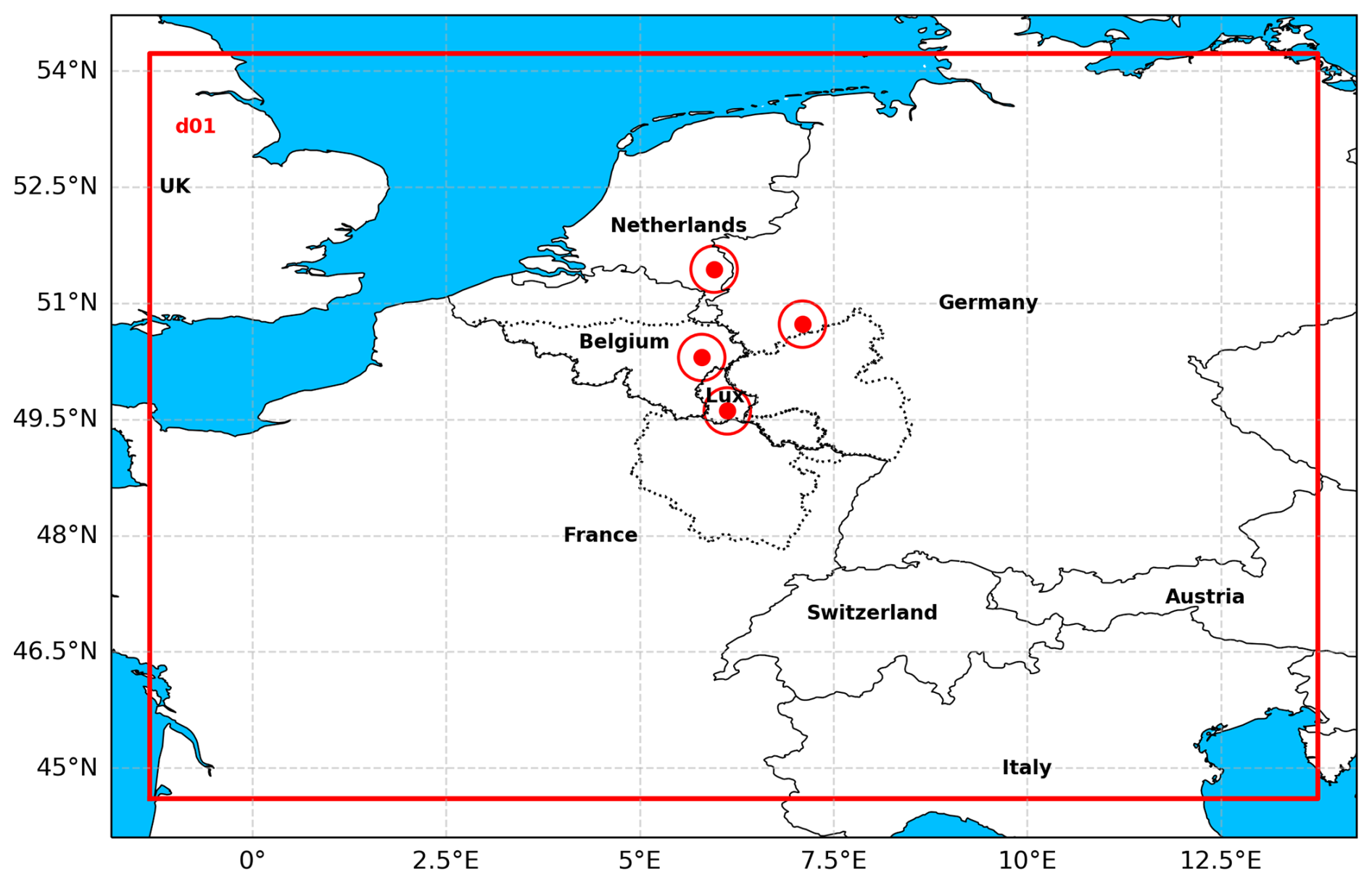
Figure 1 Map highlighting WRF Domain and areas affected by the 2021 European floods in Belgium, Germany, Luxembourg, and the Netherlands, marked with red dots and circles whereas the greater region is highlighted with dotted line Map data: coastline, national borders and sea from Natural Earth (Natural Earth, 2026); Greater Region outline from GADM (GADM, 2026).

The Weather Research and Forecasting (WRF) model is a numerical weather prediction system that, at convection-permitting resolution, can simulate the convective cells and heavy rainfall that lead to flash floods, as demonstrated in studies over Korea by Hong and Lee (2009). Although GNSS data were not assimilated, their study highlighted the importance of high-resolution modeling and accurate convective parameterization for capturing squall line formation and thunderstorm evolution, laying groundwork for future assimilation studies. The WRF Data Assimilation (WRF-DA) system, including the data assimilation module, incorporates observational data using techniques like 3D-Var to enhance short-term precipitation forecasts. In Italy, Torcasio et al. (2023) demonstrated that assimilating GNSS ZTD significantly improved both precipitable water vapor (PWV) and precipitation forecasts, especially during convective events. The study used a dense GNSS network and found that ZTD assimilation reduced forecast bias and enhanced spatial accuracy of rainfall predictions. Giannaros et al. (2020) assessed GNSS ZTD assimilation during high-impact rainfall events over Greece. Their results showed that ZTD assimilation led to better alignment with observed rainfall intensities and distributions, particularly for convective systems. The study used over 48 GNSS stations and found improvements in both forecast timing and magnitude. Poletti et al. (2019) combined radar nowcasting with numerical forecasts to improve very short-range hydrological prediction over northern Italy. Their hybrid approach enhanced rainfall field accuracy within the first 6 h, which is critical for flash flood prediction. That study combines radar nowcasting with numerical forecasts rather than assimilating zenith delays, and is cited here for the wider context of short-range rainfall prediction. Beyond these case studies, GNSS ZTD assimilation has been taken into operational practice at several centres: Bennitt and Jupp (2012) assimilated GPS ZTD operationally in the Met Office models and reported small but consistent improvements in humidity and precipitation scores, Lindskog et al. (2017) assimilated ZTD from a Nordic processing centre in HARMONIE-AROME, and Guerova et al. (2016) review the state of ground-based GNSS meteorology across Europe, including the network density and latency requirements that operational assimilation imposes. In Bulgaria, Vladimirov et al. (2020) assimilated conventional observations, satellite atmospheric-motion vectors and GNSS radio-occultation refractivity for a winter cyclone using the WRF-ARW model, finding improved mesoscale precipitation forecasts, especially in complex terrain. That study is included here for the broader context of moisture-related assimilation rather than as a ground-based zenith-delay experiment.

Despite this growing body of work, GNSS ZTD assimilation studies have concentrated on regions with dense national GNSS networks, and many report skill for selected episodes rather than over a month of repeated assimilation cycles, and no study to date has systematically quantified the added value of GNSS ZTD assimilation over Luxembourg and the Greater Region. The present study addresses this gap by performing a month-long 3D-VAR assimilation experiment covering the June–July 2021 flood period, in which an analysis is produced every six hours from a background anchored to the concurrent GFS analysis (Sect. 3.2), in which conventional observations (CONV), GNSS ZTD, and their combination (CONV + ZTD) are assimilated separately and benchmarked against a no-assimilation control. This study is designed to answer the following questions: (i) Does assimilating GNSS ZTD and/or conventional observations measurably improve WRF precipitation and temperature forecasts over Luxembourg and the Greater Region during an extreme flood event? (ii) How do conventional and GNSS ZTD observations compare, and do they play complementary roles for precipitation vs. temperature? (iii) Does combining both observation types (CONV + ZTD) yield a more balanced and stable forecast than either source alone? (iv) Given that the spatial footprint of the GNSS moisture signal is small, is its impact on regional-scale precipitation and temperature forecasts still significant when assessed over a full month of 6-hourly assimilation rather than for a single case?

2 Data

2.1 Study area: Luxembourg and the Greater Region

The Greater Region features diverse landscapes, including the densely forested Ardennes massif, the rolling hills of the Oesling in northern Luxembourg, and the fertile lowlands of the Gutland in southern Luxembourg. The Ardennes massif has a mean altitude of about 400–500 m. The Oesling, part of the Ardennes, averages around 450 m. The Gutland, with gentler hills, has a mean altitude of approximately 200 m (Lucius, 1948; Muller, 1980; Waterlot et al., 1973). The area's climatic conditions are characterized by a warm oceanic maritime climate with moderate to heavy rainfall throughout the year.

The Greater Region encompasses vital river systems, including the Moselle, Sauer, and Our, which are essential water sources and prone to seasonal flooding due to heavy rainfall. In Luxembourg, these rivers support agriculture and urban areas. In Belgium, the Semois and Ourthe rivers contribute to water supply and face similar flood risks. Germany's Moselle and Sauer rivers sustain local ecosystems and industry, with flooding challenges. In France, the Moselle and Meurthe rivers are critical for water resources, also experiencing periodic floods. Figure 2 shows the Greater Region with rivers and topography.

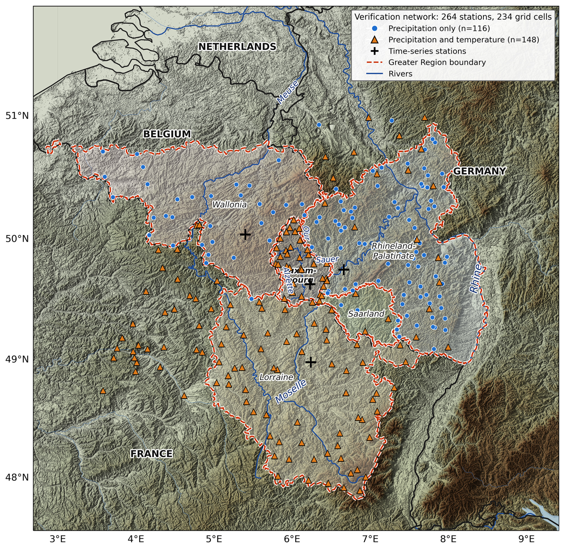
Figure 2 Topographic map of the study area showing major rivers (Rhine, Moselle, Alzette, S$\widehat{\mathrm{u}}$re, and Our), the greater region in dotted line and the locations of meteorological stations used for validation. Verification uses 264 stations withheld from the assimilation, each at least one 12 km grid length from every SYNOP position assimilated in any of the 124 observation-input files spanning the study window, and the Belgian gauges additionally from every assimilated GNSS site; together they occupy 234 distinct model grid cells. They comprise 34 stations in Luxembourg (Administration des Services Techniques de l'Agriculture, 2021), 33 in Belgium (Service Public de Wallonie, 2021), 105 in Germany (Deutscher Wetterdienst, 2021) and 92 in France (Météo-France, 2021). All 264 supply precipitation; 148 of them also report 2 m temperature (all 34 in Luxembourg, 22 of the 105 in Germany and all 92 in France), so the temperature comparison rests on that subset, and those stations are drawn with triangles. The plus (+) signs represent the stations whose time series are plotted in Sect. 2 (WALF in Luxembourg, ARLO in Belgium, DILL in Germany, and THNV in France). Map data: relief from the SRTM 1 arc second elevation model (NASA JPL, 2013); Alzette, S$\widehat{\mathrm{u}}$re and Our from the watercourse network of the Administration de la gestion de l'eau, Luxembourg; other rivers from HydroRIVERS (Lehner and Grill, 2013); national borders, coastline, lakes and the outline of Luxembourg from Natural Earth (Natural Earth, 2026); other regional outlines from GADM (GADM, 2026).

Average annual temperatures range from 8 to 12 °C and annual rainfall from 700 to 1200 mm, distributed fairly evenly through the year (Cammalleri et al., 2018).

2.2 The July 2021 flood event

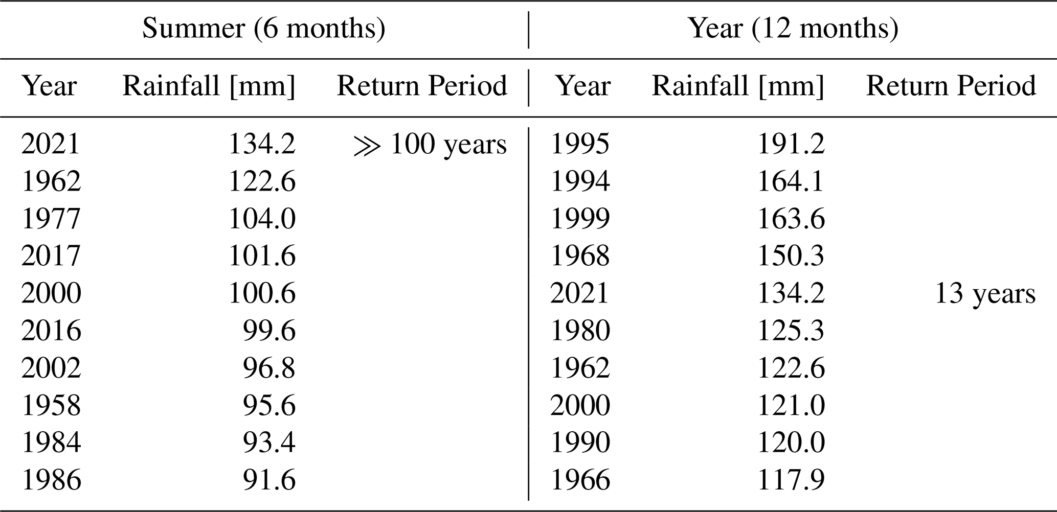
The discharge levels at the Rhine tributaries and rivers across these countries, including Luxembourg, were up to four times larger than any previously recorded events, leading to significant devastation. The flood caused 253 fatalities and more than USD 45.8×10⁹ in damages (EM-DAT, 2021). The primary cause of the flood was heavy rainfall over a short period, overwhelming existing flood defenses and catching local experts by surprise (Bertola et al., 2023; Apel et al., 2022; Kreibich et al., 2022). For the initial analysis of the 14–15 July 2021 hydrometeorological event, rainfall data were compiled from the nearby Belvaux and Obercorn stations, providing a 67-year record of daily observations maintained by the Administration of Technical Agricultural Services (Luxembourg Institute of Science and Technology (LIST), 2021). The resulting rainfall–discharge record for the Bibeschbach catchment is shown in Fig. 3, and the ranked daily and seven-day rainfall totals from this series, together with their return periods, are listed in Tables 1 and 2 respectively. The July 2021 flood was characterized by extraordinary precipitation levels, with a daily rainfall total of 68.1 mm observed at Oberkorn, Luxembourg, on 14 July. Referred to the daily series (Table 1), this total corresponds to a return period of 92 years for the summer season (April–September) and 43 years for the full hydrological year, indicating its rarity. Prior to the flood, the Bibeschbach catchment area was highly saturated, nearly double the average, increasing flood risk. The seven-day cumulative total of 134.2 mm (9–15 July) was also exceptional but, being a different accumulation period, carries different return periods: well over 100 years when referred to the summer season and 13 years when referred to the full hydrological year (Table 2). The Bibeschbach showed an immediate and intense hydrological response, with peak flows significantly higher than previous records. Other basins, such as Weierbach and Huewelerbach, experienced varying degrees of hydrological stress. Peak flow events had return periods exceeding 50 years, and in some cases over 100 years, across several watersheds, underscoring the event's exceptional nature (Luxembourg Institute of Science and Technology (LIST), 2021).

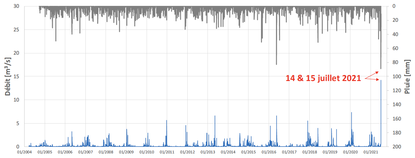
Figure 3 Bibeschbach watershed (Livange) – time series [2004–2021] of precipitation at Livange (grey bars, right-hand axis, plotted downwards) and discharge (blue line, left-hand axis). The figure is reproduced unaltered from Luxembourg Institute of Science and Technology (LIST) (2021) and therefore retains its original French labelling: Débit denotes discharge (m³ s⁻¹), Pluie denotes rainfall (mm), and the annotation 14 and 15 juillet 2021 marks 14–15 July 2021, the peak of the flood event. Source: LIST, 2021 (Luxembourg Institute of Science and Technology (LIST), 2021).

Table 1 The 10 highest daily rainfall events from the Belvaux-Obercorn observation series, with return periods for the maximum daily rainfall recorded on 14 July 2021 (covering both the summer season [April–September] and the full hydrological year [12 months]). Source: LIST, 2021 (Luxembourg Institute of Science and Technology (LIST), 2021).

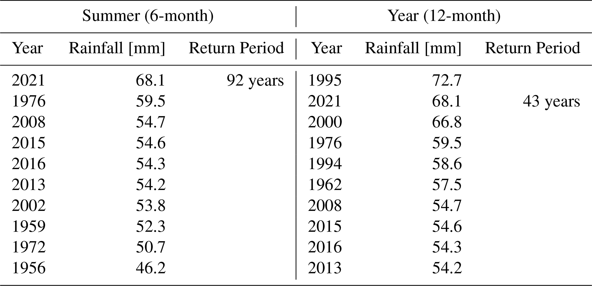
Table 2 The 10 highest seven-day cumulative rainfall totals from the Belvaux-Obercorn observation series (a different accumulation period from Table 1, and therefore not directly comparable with it) with return periods for the maximum seven-day total of July 2021 (9–15 July 2021], covering both the summer season [April–September] and the full hydrological year [12 months]. Source: LIST, 2021 Luxembourg Institute of Science and Technology (LIST), 2021.

2.3 Model forcing and observations

The National Center for Environmental Prediction (NCEP) Global Forecast System (GFS) analysis and forecast data were used as initial and boundary conditions. The GFS dataset had a spatial resolution of 0.5°×0.5° and a temporal resolution of 6 h. All four daily GFS analysis cycles (00:00, 06:00, 12:00, and 18:00 UTC) were used, each assimilation cycle being driven by the GFS analysis valid at the corresponding time rather than by a single daily cycle. These data are stored in the Research Data Archive (RDA) at UCAR https://rda.ucar.edu/ (last access: 11 November 2026).

Conventional observational data, used for assimilation, including Surface Synoptic Observations (SYNOP), Radiosonde Temperature Profiles (TEMP), and Tropospheric Airborne Meteorological Data Reporting (TAMDAR) (Daniels et al., 2006), for June and July 2021 were obtained from the ECMWF archive (Hersbach et al., 2020). To avoid ambiguity: these are the raw observational reports, retrieved in BUFR form and converted to LITTLE_R for WRFDA, and not gridded ERA5 reanalysis fields. ERA5 assimilates the same underlying reports, but no reanalysis field was ingested by WRFDA in this study. Meanwhile, Zenith Total Delay (ZTD) data was acquired from the Nevada Geodetic Laboratory (NGL) (Blewitt et al., 2018).

The precipitation data used for comparison in this study was obtained from the NASA Earthdata Global Precipitation Measurement (GPM) Integrated Multi-satellite Retrievals for GPM (IMERG) Final Run. This product delivers gauge-calibrated precipitation estimates with a spatial resolution of 0.1°×0.1° and a temporal resolution of 30 min (Huffman et al., 2023).

Radar-based quantitative precipitation estimates from the RADFLOOD21 product (Goudenhoofdt et al., 2023) were also utilized for validation purposes. This dataset provides precipitation fields with high spatial (1 km) and temporal (5-min and hourly) resolution, derived from carefully processed weather radar measurements merged with rain gauge observations. The data, provided in HDF5 format, was processed to extract precipitation values over a 6 h period, which were subsequently used for model validation.

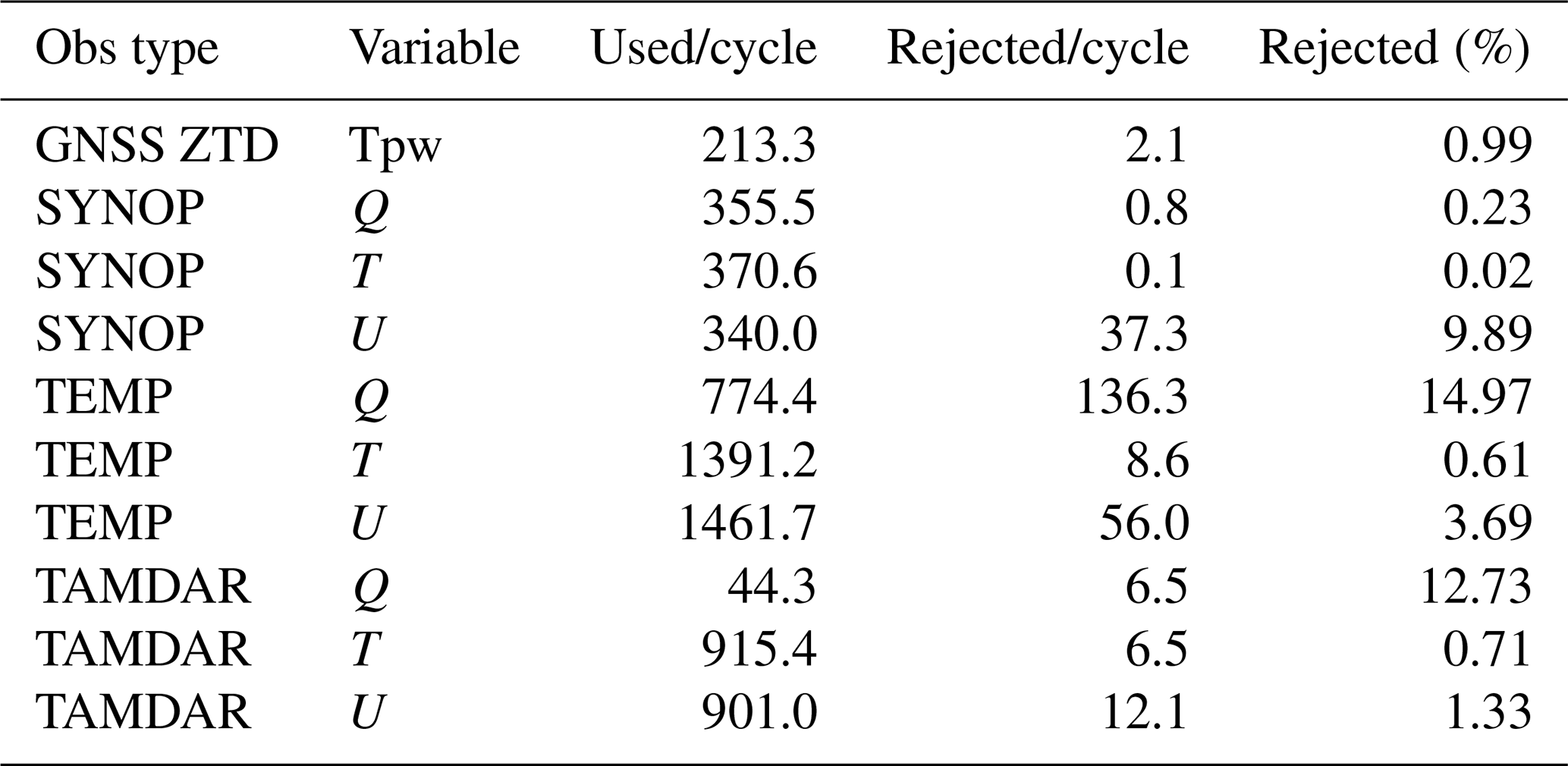
The measured meteorological parameters of the surface stations used for validation were collected from the AgriMeteo network inside Luxembourg. Surface (SYNOP) observations from 20 June to 20 July 2021 outside Luxembourg but within our study area were obtained from the NOAA Integrated Surface Database (ISD) (NOAA National Centers for Environmental Information, 2001). The data have a temporal resolution of 1 h. The locations of the observed stations used for validation, with elevation data, are shown in Fig. 2. Verification observations are drawn from a different source than the observations ingested by WRFDA, which took its conventional data from the ECMWF archive. The independence of the two sets was tested rather than assumed: every assimilated SYNOP report in all 124 obs_gts files was matched by coordinate against every candidate verification station. That test disqualified thirteen of the thirty-four AgriMeteo and NOAA ISD stations, five of them lying within 1 km of a station assimilated in essentially every cycle. The verification network was therefore rebuilt from four national providers and screened station by station, as described in Sect. 2.4; all statistics in Sect. 5 are computed on the resulting 264-station network. The assimilated network comprises on average 369 SYNOP surface reports, 1462 radiosonde levels, 901 TAMDAR reports and 213 GNSS ZTD observations per cycle after quality control (Table 3). Three counts appear in this paper and refer to different things. The observation archive holds 124 obs_gts files spanning the study window, and the independence screening uses all of them. Of these, 122 correspond to analysis cycles that ran to completion in every one of the seven configurations, and the diagnostics in observation space of Sect. 5.3 are accumulated over those 122. Each cycle produces one verified 6 h forecast, and 121 of those valid times are common to all seven configurations; the forecast verification of Sect. 5 is restricted to these 121 so that every configuration is scored on an identical sample and the comparison remains paired.

Table 3 Mean number of observations assimilated per cycle after quality control, and mean number rejected. Each row is averaged over the cycles in which that observation type was reported rather than over all 122 cycles: GNSS ZTD and the SYNOP variables are present in all 122, the TAMDAR wind and temperature reports in 120, and TAMDAR humidity in only 43, so its 44.3 reports per cycle is a mean over reporting cycles and corresponds to 15.6 spread over the whole period. GNSS ZTD is handled through the WRFDA gpspw slot. Counts are identical for CV3 and CV5 because both share the same background and therefore the same innovations at the quality-control step.

2.4 Verification network

Verification requires stations that the assimilation has not already seen. Synoptic stations are unsuitable for this purpose, because they are the observations being assimilated: a verification network drawn from the synoptic network cannot measure forecast improvement without circularity. The network used here is therefore built from the openly available national networks that operate independently of the synoptic feed.

Four providers contribute. Inside Luxembourg, the agrometeorological network of the Administration des Services Techniques de l'Agriculture supplies hourly precipitation and 2 m temperature (Administration des Services Techniques de l'Agriculture, 2021). Over Germany, hourly precipitation is taken from the Climate Data Center of the Deutscher Wetterdienst (Deutscher Wetterdienst, 2021), and over France from the données climatologiques de base of Météo-France (Météo-France, 2021). Over Belgium the five-minute rain-gauge network of the Service Public de Wallonie (Service Public de Wallonie, 2021) is used. The automatic weather stations of the Royal Meteorological Institute of Belgium (Royal Meteorological Institute of Belgium, 2021) were examined first but could not be used at all: every one of the fourteen matches the identifier of an assimilated SYNOP station, so the Belgian AWS network is in effect the Belgian SYNOP network. The SPW hydrological network is separate from the synoptic network and is therefore the only route to independent Belgian verification.

Every candidate station was screened before being admitted, and before being downloaded where the provider serves one file per station. A station is accepted only if it lies at least one 12 km grid length from every SYNOP report assimilated at any of the 124 observation-input files spanning the study window. The assimilated set is not constant: it varies between 1273–1351 stations per cycle and comprises 1361 distinct stations over the month, so the test uses the union across all cycles rather than a single snapshot. The SYNOP test is the one that matters for independence, because a withheld surface report is the same quantity that would otherwise have been assimilated. Proximity to an assimilated GNSS receiver is a different matter: zenith total delay is a column-integrated refractivity, whereas the verifying observation is a surface accumulation or a 2 m temperature, and neither was ingested. We nevertheless applied the 12 km rule against the 234 assimilated GNSS sites to the Belgian gauges as well, as the most conservative selection available for a network added late in the study; it removes 28 of the 61 Belgian gauges that pass the SYNOP test. Applying the same rule to the whole network would remove a further 96 stations, 24 of the 34 in Luxembourg, 50 of the 105 in Germany and 22 of the 92 in France. We report in Sect. 5.9 what happens when it is: the conclusions do not change, which is the evidence that GNSS proximity is not a source of dependence here. Identifier matching was deliberately not used across networks: six German station numbers coincide with assimilated WMO identifiers while lying 690–790 km away, so only coordinates provide a valid test.

This network verifies precipitation. The near-surface temperature comparison of Sect. 5.6 uses the 148 of them that also report 2 m temperature, and its scope is stated there. The resulting precipitation network, shown in Fig. 2, comprises 264 stations: 34 in Luxembourg, 33 in Belgium, 105 in Germany and 92 in France. Because stations sharing a 12 km grid box are handed an identical model value and are therefore not independent samples of model error, the effective size is better expressed as the 234 distinct grid cells they occupy. The 33 Belgian gauges each fall in a grid cell that no other station uses, so they add 33 genuinely new cells rather than duplicating existing ones. All timestamps were converted to UTC before aggregation; the AgriMeteo export is in local time and required a −2 h shift, the German and French archives are already in UTC, and the Belgian five-minute values were requested with UNIX-millisecond timestamps, which are unambiguous. The alignment was verified rather than assumed: for each network the lag correlation between network-mean observed and network-mean modelled precipitation peaks at zero lag. Six-hourly totals were then formed with the same backward window used throughout this study, each Belgian total requiring all 72 five-minute values to be present.

2.5 Observation pre-processing

Conventional data from ECMWF was provided in BUFR format, which was then converted to LITTLE_R format. LITTLE_R is an ASCII-based observation file format designed as an intermediate format to enable WRFDA to assimilate a wide range of observation types in a standardized manner. It is a report-based format and is also the format used by OBSPROC which is a WRFDA utility. The OBSPROC utility was employed to filter out unnecessary data beyond the model domain. Stations used for assimilation are shown in Fig. 4. WRFDA's own quality control rejected on average 2.1 of the 215.4 ZTD reports submitted per cycle, or 1.0 %, leaving on average 213 of 215 per cycle.

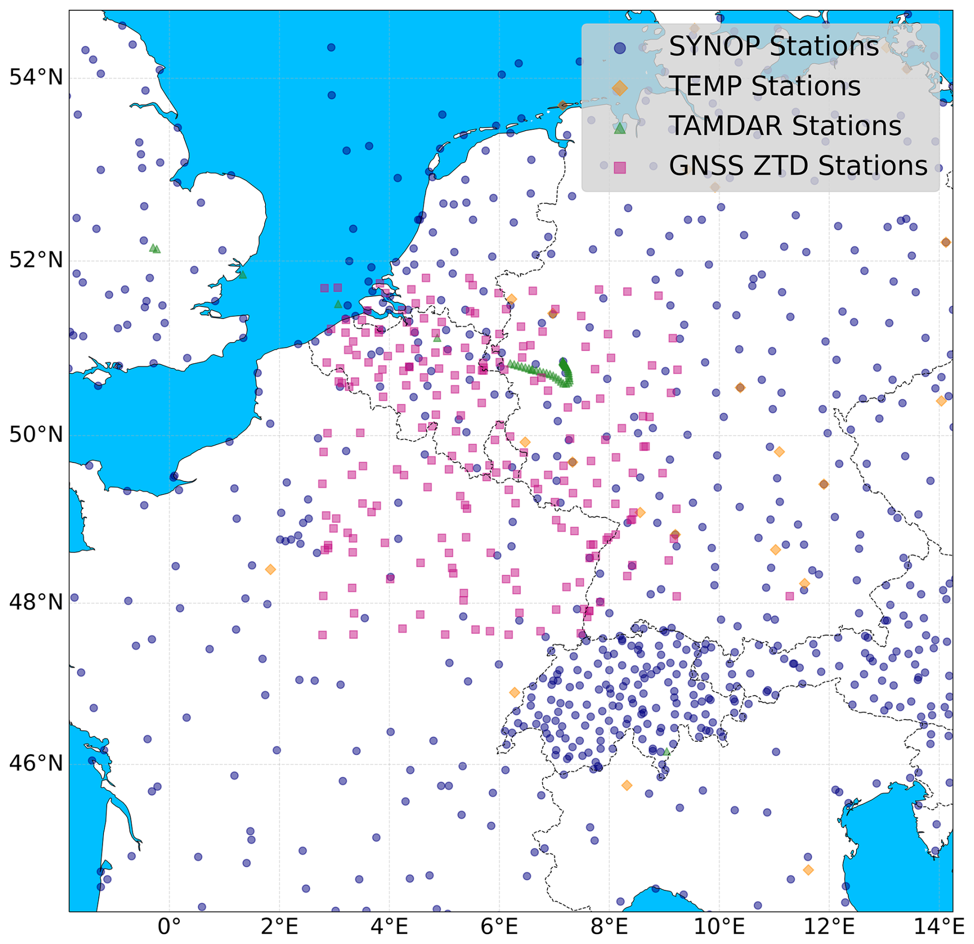
Figure 4 Stations locations for assimilation.

To extract and process the NGL Zenith Total Delay (ZTD) data, compressed ZIP archives containing trop.gz files were systematically unpacked and parsed. These files contain yearly data with a temporal resolution of 5 min. Data corresponding to June and July 2021 were filtered at a 6 h interval based on file metadata, and ZTD values were extracted and converted from millimetres to centimetres. The flow chart for the observed data pre-processing is shown in Fig. 5.

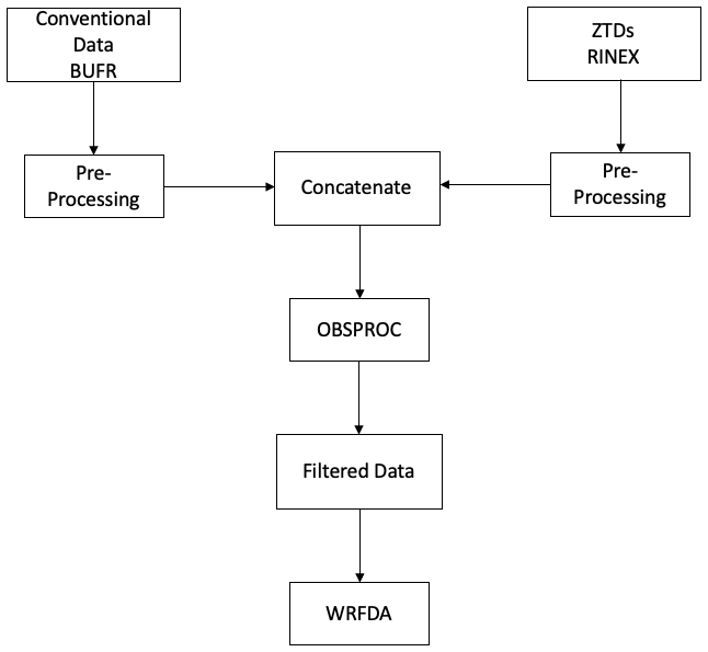
Figure 5 Pre-processing flow chart showing the integration of ECMWF BUFR and GNSS ZTD data, followed by filtering via OBSPROC for WRFDA assimilation.

The NGL ZTD estimates are derived from a precise-point-positioning (PPP) processing of the GNSS observations using the GipsyX software, and each estimate is accompanied by a formal uncertainty. Over the study period and network, this formal uncertainty was at the sub-centimetre level, with a median of approximately 1.7 mm and values ranging from about 1.3–4.3 mm, confirming the high quality and consistency of the ZTD observations used for assimilation. Epochs whose reported formal uncertainty was anomalously large were discarded during pre-processing. The processing log records that this step was applied but not the numerical threshold, which is therefore not stated here. The rejection counts given in Table 3 are a different quantity, being WRFDA's own quality-control rejections at the assimilation step, and should not be read as the size of this pre-processing filter. The formal uncertainties reported by the archive over this network and period have a median of about 1.7 mm and a range of 1.3–4.3 mm, so the step can have removed only a small number of outliers. In the WRFDA cost function, a uniform observation error of 8 mm (0.8 cm) was assigned to all ZTD observations. This value is deliberately larger than the formal GNSS processing uncertainty because the observation error in data assimilation must additionally account for representativeness error and observation-operator (forward-model) error, including the mapping of the slant/zenith delay onto the model column and the sensitivity of the delay to the model humidity, temperature, and station-height representation. The chosen value of 8 mm lies within the accuracy range recommended for ZTD products used in numerical weather prediction under the E-GVAP standards (optimal 5 mm, target 10 mm) and is comparable to the ∼7.6 mm ZTD accuracy reported for a similar WRFDA ZTD assimilation study over Greece (Giannaros et al., 2020).

To illustrate the temporal variability during the 2021 European floods, Fig. 6 shows surface pressure, Fig. 7 displays temperature, and Fig. 8 presents zenith total delay (ZTD) from 20 June to 20 July 2021 (days 171–201). Due to space constraints, we plot one station per country: Luxembourg (WALF/6590), Belgium (ARLO/6476), Germany (DILL/10609), and France (THNV/7093). These reveal coordinated drops in pressure and rises in ZTD around mid-July, aligning with the flood event.

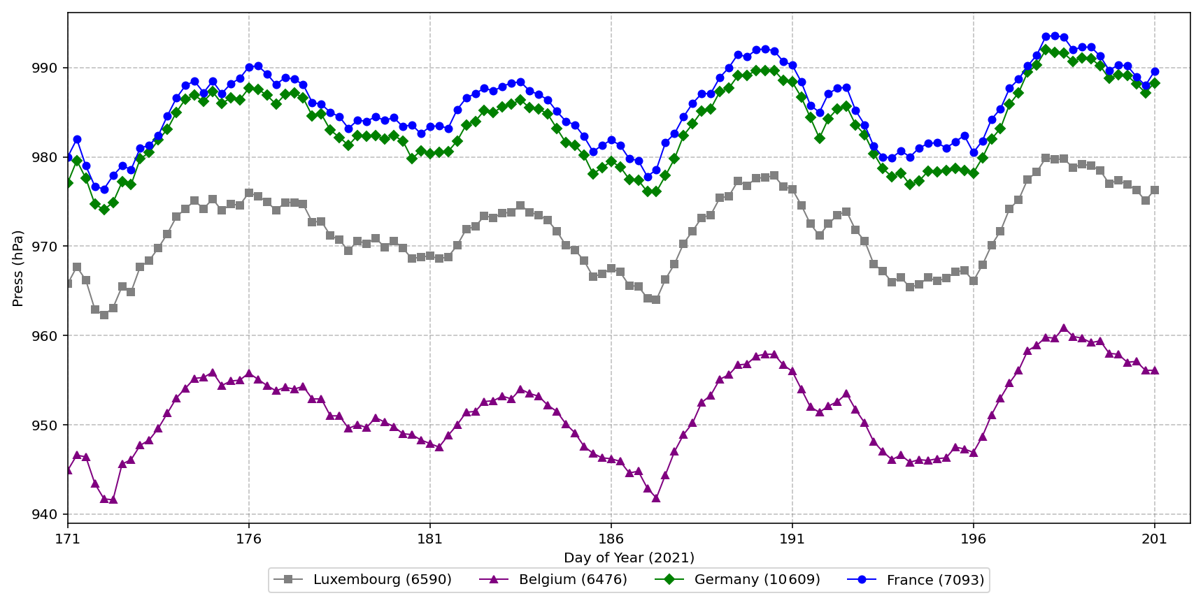
Figure 6 Time series of surface pressure (hPa) at representative stations (one per country) from 20 June to 20 July 2021, highlighting regional atmospheric variability preceding the flood event. Pressure values are shown without altitude correction.

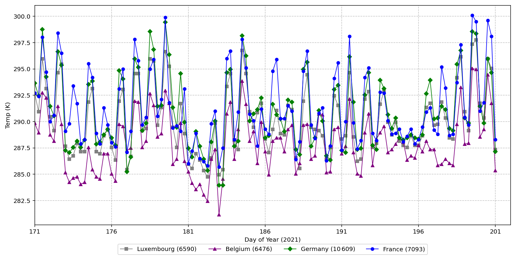
Figure 7 Time series of near-surface temperature (K) at representative stations (one per country) from 20 June to 20 July 2021, capturing thermal dynamics preceding the flood event. Stations temperatures are shown without altitude correction.

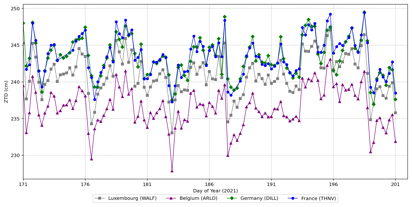
Figure 8 Time series of Zenith Total Delay (ZTD, cm) at GNSS stations (one per country) from 20 June to 20 July 2021, indicating atmospheric moisture variations preceding the 2021 European floods. ZTD values are shown without altitude correction.

3 Model and Experimental Design

3.1 The WRF model and its configuration

The physical parameterizations listed in Table 4 were not tuned for this study. They follow the configuration adopted in earlier WRF applications over the Greater Region and are held fixed across all experiments, so that any difference between experiments is attributable to the assimilation rather than to the physics. A systematic physics sensitivity study for this domain remains outstanding and is noted in Sect. 6.

(Thompson et al., 2008)(Mlawer et al., 1997)(Dudhia, 1989)(Jiménez et al., 2012)(Tewari et al., 2004)(Hong et al., 2006)(Grell and Freitas, 2014)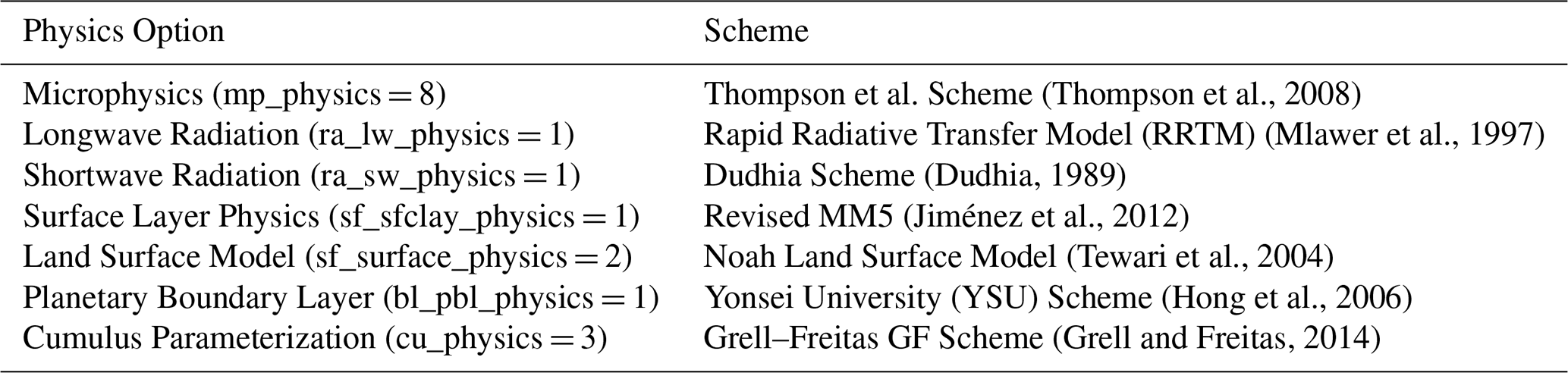

Table 4 WRF physical parameterizations for domain d01.

The Weather Research and Forecasting (WRF) model is a next-generation mesoscale numerical weather prediction system, developed collaboratively by the National Center for Atmospheric Research (NCAR), the National Centers for Environmental Prediction (NCEP), the National Oceanic and Atmospheric Administration's Forecast Systems Laboratory (NOAA-FSL), and other research institutions (Skamarock et al., 2019)

It comprises two core model frameworks: the Advanced Research WRF (ARW), designed by NCAR using Eulerian mass coordinates for research applications, and the Nonhydrostatic Mesoscale Model (NMM), developed by NCEP for operational forecasting. The WRF model is routinely applied at horizontal grid spacings from a few hundred metres to tens of kilometres; a single 12 km domain is used here (Sect. 3.2). WRF provides a versatile platform for research in weather, climate and disciplines in related categories, and plays an important role in practical weather forecasting and risk management. The spatial configuration of the model is given in Table 5 and the physical parameterizations in Table 4.

(Friedl and Sulla-Menashe, 2022)(Didan, 2021)(National Centers for Environmental Prediction (NCEP), 2025)

Table 5 Spatial parameter of the WRF Model used in this study.

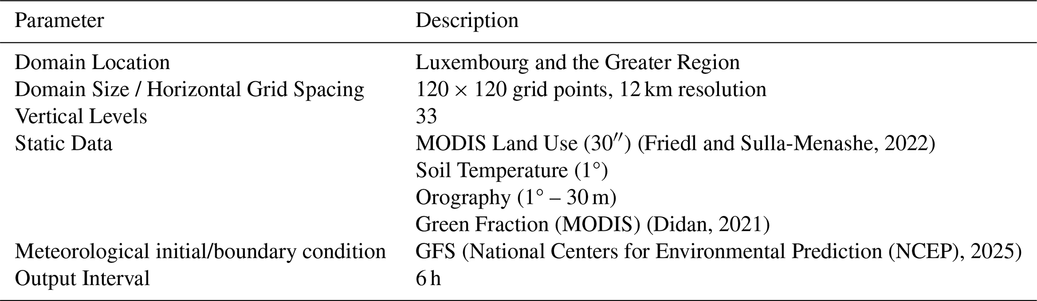
Note: MODIS (Moderate Resolution Imaging Spectroradiometer) is a NASA satellite instrument providing land use and vegetation data for the WRF model. whereas GFS (Global Forecast System) is a global numerical weather prediction model developed by the National Centers for Environmental Prediction (NCEP), providing atmospheric initial and boundary conditions for WRF simulations.

A single computational domain with a horizontal grid spacing of 12 km was adopted in this study. This choice reflects a deliberate balance between spatial detail and the computational demands of the experimental design. Because the central objective is to isolate the added value of data assimilation, the model was run as a month-long sequence of independent 6 h analysis/forecast cycles: at each analysis time T it starts from the GFS analysis valid at T−6 h, a 6 h forecast supplies the first guess at T, the observations are assimilated at T, and the analysis initialises the forecast to T+6 h that is verified. The analysis is not carried into the next cycle, so the cycles do not accumulate. Each of the seven configurations (No DA, and CONV, ZTD, and CONV + ZTD with each of two background error covariances) was repeated over every assimilation cycle. Performing month-long, seven-fold cycled assimilation at convection-permitting resolution (≤4 km) would have been computationally prohibitive, whereas the 12 km configuration makes the full experimental matrix tractable while still resolving the synoptic and meso-β scale features that governed the July 2021 event. The domain is also large enough to encompass the entire Greater Region together with the surrounding GNSS network of 234 stations whose ZTD observations are assimilated, ensuring that the moisture information propagates within, rather than across, the lateral boundaries. Furthermore, the 12 km grid is consistent with the 0.5° resolution of the GFS initial and boundary conditions and with the Grell–Freitas cumulus parameterization employed here, which is appropriate for grid spacings at which convection is not explicitly resolved. As the analysis focuses on the relative improvement of each assimilation experiment with respect to a common baseline rather than on absolute convective-scale rainfall reproduction, the 12 km resolution is well suited to the aims of this work.

3.2 WRFDA 3D-VAR data assimilation

In this study, the three-dimensional variational (3D-VAR) assimilation mode in the WRF Data Assimilation (WRFDA) system was employed for assimilating observational data. The core concept of 3D-VAR is to minimize a quadratic cost function, which quantifies the differences between the analysis field and both the observation and background fields. This objective function is mathematically expressed as Eq. (1) (Lorenc, 2003; Barker et al., 2004).

$$\begin{array}{ll}{\displaystyle }J\left(\mathit{x}\right)=& {\displaystyle }{\displaystyle \frac{\mathrm{1}}{\mathrm{2}}}(\mathit{x}-{\mathit{x}}_{\mathrm{b}}{)}^{\mathrm{T}}{\mathbf{B}}^{-\mathrm{1}}(\mathit{x}-{\mathit{x}}_{\mathrm{b}})\\ \text{(1)}& {\displaystyle }& {\displaystyle }+{\displaystyle \frac{\mathrm{1}}{\mathrm{2}}}{\left(H\left(\mathit{x}\right)-\mathit{y}\right)}^{\mathrm{T}}{\mathbf{R}}^{-\mathrm{1}}\left(H\left(\mathit{x}\right)-\mathit{y}\right)\end{array}$$

where: J(x) is the cost function minimised in the 3D-VAR framework; it quantifies the total discrepancy between the model state and both the background field and the observations, x is the model state vector (the analysis x_a is the state vector that minimises J), x_b denotes the background field, B is the background error covariance matrix, H is the forward (observation) operator, which maps model variables into observation space, y represents the observations, R is the observation error covariance matrix. Following standard WRFDA practice, R is taken to be diagonal, that is observation errors are assumed mutually uncorrelated, with the variances for each observation type and level read from the WRFDA observation-error table; the GNSS ZTD error is 0.8 cm, the value carried in the LITTLE_R records. No observation-error file was supplied to WRFDA, so the variances are those of the model's own built-in table for each type and level; the configuration is reproducible from the run script archived with this study, which sets ob_format=2 and supplies the ZTD error in the observation records themselves. Gross-error rejection discards a departure whose magnitude exceeds a fixed multiple of the assigned observation error, the multiples being 𝚖𝚊𝚡_𝚎𝚛𝚛𝚘𝚛_𝚝=4.0, 𝚖𝚊𝚡_𝚎𝚛𝚛𝚘𝚛_𝚞𝚟=3.0, 𝚖𝚊𝚡_𝚎𝚛𝚛𝚘𝚛_𝚝𝚋=3.0, 𝚖𝚊𝚡_𝚎𝚛𝚛𝚘𝚛_𝚛𝚏=3.0, 𝚖𝚊𝚡_𝚎𝚛𝚛𝚘𝚛_𝚛𝚟=2.5, 𝚖𝚊𝚡_𝚎𝚛𝚛𝚘𝚛_𝚚=1.5 and 𝚖𝚊𝚡_𝚎𝚛𝚛𝚘𝚛_𝚙𝚠=5.0, the last governing the GNSS delays. The assigned ZTD error is 0.800 cm in every archived observation record and can be recovered independently from the archived cost-function diagnostics, where σ_o inferred from J_o and the analysis departures is 0.800 cm, confirming the value quoted above.

Seven configurations were run over the full study period (20 June–20 July 2021) using an identical model configuration and differing only in the observations assimilated and in the background error covariance. Four observation configurations were used: (i) a control run with no data assimilation (CTRL, referred to as No DA in the figures), initialised and driven solely by GFS; (ii) assimilation of conventional observations only (CONV); (iii) assimilation of GNSS ZTD only (ZTD); and (iv) assimilation of both observation types together (CONV + ZTD). The assimilation follows a rapid-update strategy in which every analysis is anchored to the concurrent global analysis, shown schematically in Fig. 9. Observations are assimilated at the four synoptic times 00:00, 06:00, 12:00, and 18:00 UTC each day. At each analysis time T the model is re-initialised from the GFS analysis valid at T−6 h, a 6 h WRF forecast provides the background, WRFDA combines that background with the observations to produce an analysis, and the analysis initialises the 6 h forecast valid at T+6 h that is verified. Lateral boundary conditions are taken from GFS at each cycle. The analysis is not carried over to the following cycle: each cycle begins again from the GFS analysis valid at that time. This design is deliberate. It prevents model drift from accumulating over a month-long experiment, and it means that all seven configurations share an identical background at every analysis time, so that every difference between them arises from the assimilation step alone rather than from trajectories that have gradually diverged. It also means that the assimilation increments do not compound from one cycle to the next, which is relevant when interpreting the magnitude of the impacts reported in Sect. 5 and is discussed in Sect. 6. The No DA control consists of the same GFS-initialised 6 h forecasts without any observations ingested.

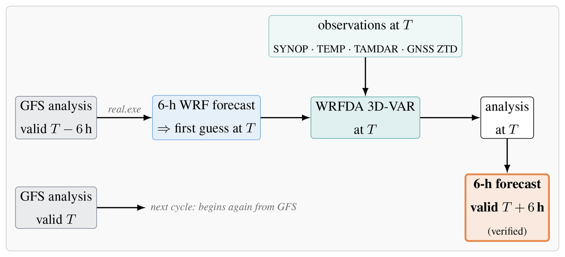
Figure 9 The 6-hourly analysis/forecast cycle used in this study. At each analysis time T the model is re-initialised from the GFS analysis valid at T−6 h; a 6 h WRF forecast supplies the first guess at T; WRFDA 3D-VAR combines it with the observations valid at T; and the resulting analysis initialises the 6 h forecast valid at T+6 h, which is the field verified against the station network. The next cycle begins again from the GFS analysis valid at T. All experiments therefore share an identical first guess at every analysis time, and differ only through which observations enter the 3D-VAR step. The No DA control consists of the first-guess forecasts alone, with the 3D-VAR step omitted.

The CV3 background error covariance option was used in WRFDA, which incorporates climatological background error statistics derived from a global NCEP/NCAR reanalysis dataset (Barker et al., 2004). This configuration represents a precomputed, static estimate of background error covariances based on long-term global forecasts and is commonly provided by NOAA as part of the operational WRFDA package. CV3 was selected deliberately because it is domain-independent and does not require the generation of a case-specific background error matrix (e.g. via the NMC method or an ensemble, as needed for the CV5 option). This provides a controlled, reproducible, and widely used baseline against which the impact of each observation type can be isolated and fairly compared, without introducing an additional degree of freedom from a locally tuned B matrix. It is nevertheless acknowledged that CV3, being climatological and homogeneous, is not the ideal choice for a precipitation-focused study, as it cannot represent the flow-dependent, anisotropic error structures associated with convective moisture fields. The domain-specific CV5 option is therefore tested alongside it throughout. CV5 is not flow-dependent: like CV3 it is held fixed through the assimilation, but it is derived for this domain by the NMC method from forecast differences rather than taken from a global climatology, and it is horizontally homogeneous within each vertical level. It was generated by the NMC method from differences between 24–12 h forecasts over 21 June–19 July 2021; the implications of that choice of window are taken up in Sect. 6.3. The two options are not the same covariance model tuned differently. They differ also in their control variables and in how balance between them is imposed. CV5 works with unbalanced velocity potential, temperature and surface pressure and derives the balance by regression, whereas CV3 is applied in physical space through recursive filters. The contrast reported here is therefore between two covariance formulations, of which only one is derived for this domain, and not between a tuned and an untuned version of a single formulation. Each observation configuration is repeated over the same month with cv_options=5 and an NMC-derived background error covariance, everything else being identical. Because the background is re-anchored to GFS at every cycle, the CV3 and CV5 experiments see exactly the same first guess and exactly the same observations, so the comparison between them isolates the effect of the background error covariance alone.

3.3 Extraction of model values at station locations

Model values are taken at the nearest model grid point to each station rather than interpolated. For every station the grid point minimising the great-circle distance to its coordinates is selected once and used for all variables and all experiments. At a 12 km grid length the choice between nearest-point extraction and bilinear interpolation is small compared with the representativeness error of comparing a grid-box mean with a point gauge, and nearest-point extraction has the advantage of being exactly reproducible and of making the dependence between stations explicit: the 59 stations that share a grid cell with another station receive an identical model value, which is why the bootstrap of Sect. 5.9 resamples the 234 grid cells rather than the 264 stations.

No vertical interpolation is applied to the extracted fields. Precipitation is a surface accumulation, and 2 m temperature is a diagnostic field valid at the model terrain height; the difference between model terrain and station elevation is handled explicitly by the lapse-rate correction of Sect. 4.2 rather than by interpolating between model levels.

4 Verification Methodology

To evaluate the accuracy of numerical predictions, four statistical error metrics were employed: Mean Absolute Error (MAE), Root Mean Square Error (RMSE), Symmetric Mean Absolute Percentage Error (SMAPE), and Bias. Additionally, Probability of Detection (POD) and False Alarm Ratio (FAR) (Wilks, 2006) were used to assess precipitation detection performance. These metrics provide a quantitative measure of the deviation between model predictions and observed values, defined as follows:

$$\begin{array}{}\text{(2)}& {\displaystyle }& {\displaystyle }\text{MAE}={\displaystyle \frac{\mathrm{1}}{n}}\sum _{i=\mathrm{1}}^n\left|{\widehat{y}}_i-y_i\right|\text{(3)}& {\displaystyle }& {\displaystyle }\text{RMSE}=\sqrt{{\displaystyle \frac{\mathrm{1}}{n}}\sum _{i=\mathrm{1}}^n{\left({\widehat{y}}_i-y_i\right)}^{\mathrm{2}}}\text{(4)}& {\displaystyle }& {\displaystyle }\text{SMAPE}={\displaystyle \frac{\mathrm{100}\mathit{\%}}{n}}\sum _{t=\mathrm{1}}^n{\displaystyle \frac{|{\widehat{y}}_t-y_t|}{\left(\left|{\widehat{y}}_t\right|+\left|y_t\right|\right)/\mathrm{2}}}\text{(5)}& {\displaystyle }& {\displaystyle }\text{Bias}={\displaystyle \frac{\mathrm{1}}{n}}\sum _{i=\mathrm{1}}^n\left({\widehat{y}}_i-y_i\right)\text{(6)}& {\displaystyle }& {\displaystyle }\text{POD}={\displaystyle \frac{\text{hits}}{\text{hits}+\text{misses}}}\text{(7)}& {\displaystyle }& {\displaystyle }\text{FAR}={\displaystyle \frac{\text{false alarms}}{\text{hits}+\text{false alarms}}}\end{array}$$

where n is the total number of samples, ${\widehat{y}}_i$ denotes the model-predicted value, and y_i represents the observed value. For POD and FAR, a precipitation threshold of 0.1 mm is used to define “hits” (cases where both observed and predicted precipitation exceed the threshold), “misses” (observed events above the threshold not predicted), and “false alarms” (predicted events above the threshold not observed).

To ensure that the results are statistically robust and not driven by a single event, all of the metrics above were computed over the entire one-month study period (20 June–20 July 2021) rather than for isolated dates. Each metric aggregates every 6-hourly forecast cycle across all independent validation stations within the study area, so that n comprises several thousand matched model–observation pairs for both precipitation and temperature. This large sample, spanning the full range of quiescent and extreme-precipitation conditions during the period, means that the reported differences between the experiments reflect the sustained, month-long behaviour of the assimilation rather than event-specific fluctuations, and are therefore representative of the model's general performance over the region.

In addition to this monthly aggregation, the change in mean error was assessed with a paired test. The resampling unit is the model grid cell rather than the station, for the same reason that it is in Sect. 5.9: the 264 stations occupy 234 distinct 12 km cells, and stations sharing a cell are handed an identical model value, so they are not independent samples of model error. The month-integrated mean error was therefore averaged over the stations in each cell, and for each of the six assimilating configurations the resulting cell value was paired with the corresponding value for the no-assimilation control in the same cell, and the 234 paired differences were tested with the non-parametric Wilcoxon signed-rank test. This design tests whether the direction of the change is consistent across the domain. It is applied to the mean error only; the categorical scores and the absolute-error metrics are assessed with the resampling procedures of Sect. 5.9 instead. The outcome of these tests is reported with the results in Sect. 5.4.

4.1 Categorical verification across thresholds

Probability of detection and false alarm ratio alone cannot separate a genuine gain in discrimination from a uniform increase in forecast rain frequency, since both rise together when a model simply rains more often. The categorical assessment is therefore extended in two ways. First, the frequency bias index (FBI), critical success index (CSI) and equitable threat score (ETS) are reported alongside POD and FAR,

$$\begin{array}{ll}{\displaystyle }& {\displaystyle }\text{FBI}={\displaystyle \frac{h+f}{h+m}},\mathrm{\text{CSI}}={\displaystyle \frac{h}{h+m+f}},\\ \text{(8)}& {\displaystyle }& {\displaystyle }\text{ETS}={\displaystyle \frac{h-h_r}{h+m+f-h_r}},h_r={\displaystyle \frac{(h+m)(h+f)}{n}},\end{array}$$

where h, m, f are hits, misses and false alarms, n the total number of matched pairs and h_r the hits expected by chance. FBI measures how often the model forecasts rain relative to how often it was observed. ETS adjusts the score for the hits expected by chance; it is not independent of the frequency bias, so FBI must be examined alongside it rather than treated as superseded by it. Second, all of FBI, POD, FAR, CSI and ETS are computed at six thresholds (0.1, 1, 5, 10, 20, and 30 mm per 6 h) rather than only at 0.1 mm, so that the behaviour at the higher intensities relevant to flooding can be distinguished from that at the drizzle threshold.

4.2 Height correction of near-surface temperature

The model 2 m temperature is valid at the height of the model terrain, the observation at the true station height. On a 12 km grid these differ because the model terrain is an average over the grid box, and the difference is systematic in valleys. Model temperature is therefore adjusted to the station height before verification,

$$\begin{array}{ll}{\displaystyle }& {\displaystyle }{T}_{\text{model}}^{\text{adj}}=T_{\text{model}}+\mathrm{\Gamma }(h_{\text{model}}-h_{\text{station}}),\\ \text{(9)}& {\displaystyle }& {\displaystyle }\mathrm{\Gamma }=\mathrm{6.5}\mathrm{K}{\mathrm{km}}^{-\mathrm{1}},\end{array}$$

with Γ the ICAO standard-atmosphere lapse rate, the value most commonly used in verification (Sheridan et al., 2010). Model terrain heights are taken from the HGT field at the same grid point from which the station values are extracted; station heights come from the station listing of each provider: the agrometeorological list in Luxembourg, the DWD station description file in Germany and the ALTI field of the hourly records in France. The distribution of h_model−h_station is reported in Sect. 5. The sensitivity of the results to Γ was tested over the range 5.5–6.5 K km⁻¹, bracketing the standard value. Because the mean difference between model and station height is only 14.9 m, a change of 1 K km⁻¹ in Γ shifts the network mean correction by about 0.015 K. Across the range tested the mean error of any configuration changes by at most that amount, and its mean absolute and root-mean-square errors by at most 0.005 K, an order of magnitude smaller than the differences between configurations reported in Sect. 5.6; the two configurations closest to zero mean error are the same at every value tested. The choice of Γ within this range therefore does not affect any conclusion drawn here. Surface pressure is used only qualitatively in this study, in the time series of Fig. 6, and is not corrected; the figure caption states this.

4.3 Verification in observation space

In addition to the station verification, the assimilation is assessed in its own observation space using the WRFDA diagnostics written at every cycle. For each observation type the mean and root-mean-square of the observation-minus-background departure (O−B) and the observation-minus-analysis departure (O−A) are accumulated over the month, weighted by the number of observations in each cycle, together with the number of reports accepted and rejected by quality control. This is the only diagnostic that isolates what the assimilation does to the model state independently of the forecast that follows it, and it is the natural place to verify the GNSS ZTD component in the quantity that is actually assimilated.

5 Results

To systematically evaluate the model performance, the results are structured in a comparative framework. First, the model outputs are compared against RADAR observations to assess spatial and temporal consistency. This is followed by a comparison between the model and GPM IMERG satellite estimates. The quantitative verification then rests on the independent rain-gauge network alone; radar and satellite are used for spatial comparison and not as references for the statistics. Statistical metrics are employed to quantify the accuracy and reliability of the model.

5.1 Rainfall forecast results

To analyze the rainfall patterns and distribution in the study area, as well as the impact of assimilating different data types (conventional and ZTD data) on WRF model rainfall forecasts, we first ran the model from GFS alone, without assimilation (CTRL), and then repeated it with conventional observations and NGL ZTD assimilated, separately and together. The model was run for a one-month period from 20 June to 20 July 2021. Rain-gauge observations from the four national networks of Sect. 2.4 (the Administration des Services Techniques de l'Agriculture in Luxembourg, the Service Public de Wallonie in Belgium, the Deutscher Wetterdienst in Germany and Météo-France) were used as the verification reference, with radar and NASA GPM IMERG used for spatial comparison only. Due to space constraints, instead of presenting the full monthly rainfall distribution, we illustrate a representative 6-hourly rainfall pattern for a single day (14–15 July 2021) in the study area, comparing the model forecasts before and after data assimilation which are shown in Figs. 10 and 11. This date was selected due to the intensity and spatial extent of the precipitation event, which marked a critical phase of the 2021 flood episode.

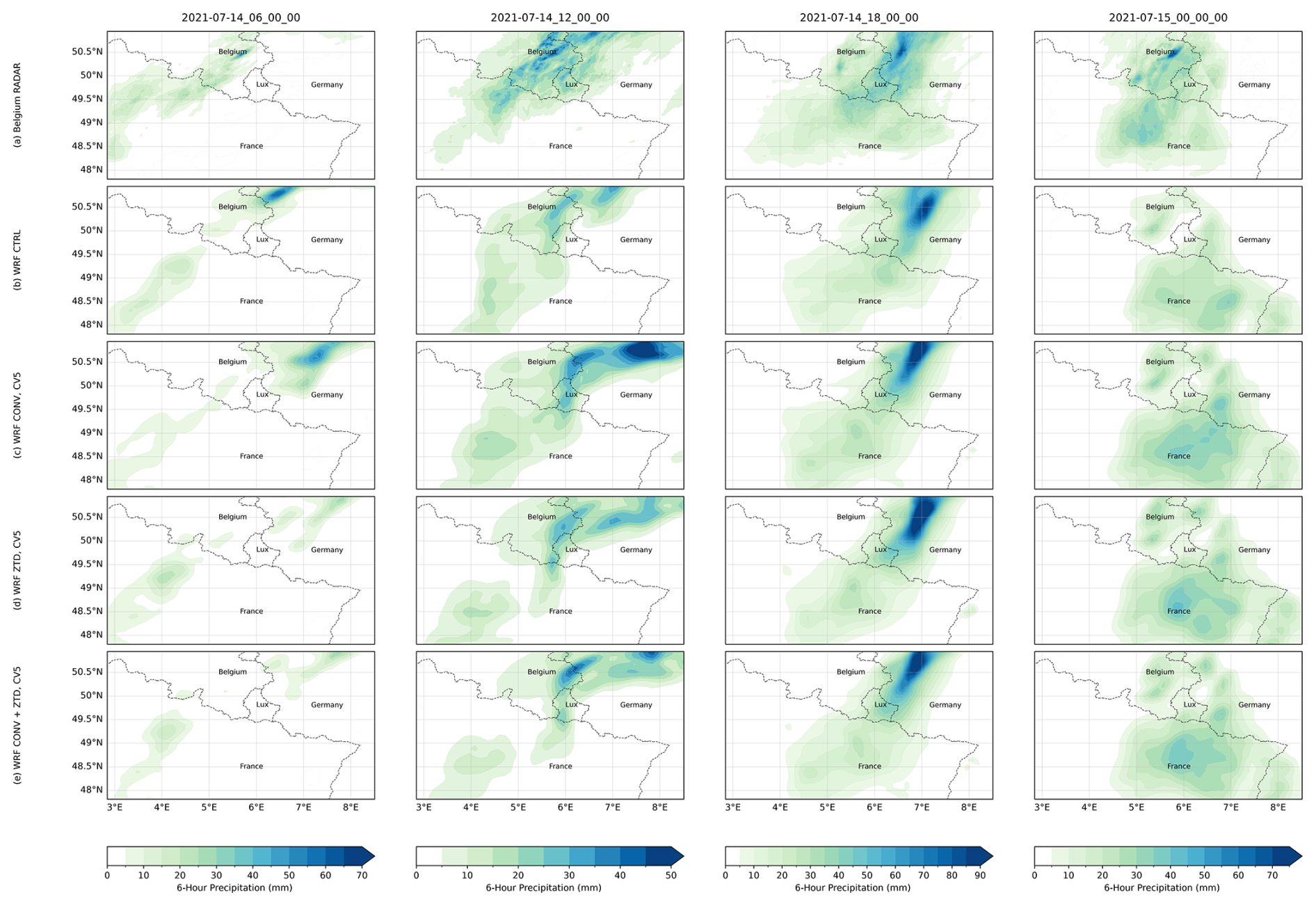
Figure 10 Spatial distribution of 6 h accumulated precipitation (mm) over the Greater Region during 14–15 July 2021, at the indicated UTC times. The assimilation experiments shown are the CV5 configurations. Panels: (a) Radar observations; (b) the no-assimilation control (CTRL); (c) CONV with CV5; (d) ZTD with CV5; (e) CONV + ZTD with CV5. Each field is drawn on its own native grid and no regridding is performed: the radar on the 700×700 1 km RADCLIM grid in EPSG:3812 with its upper-left corner at (300 000, 1 000 000), and the model on its 12 km grid. All panels show 6 h accumulations in mm. The colour scale is set separately for each time step, its maximum being the largest 6 h accumulation observed by the radar at that time, and is then applied to all five panels of that column so that model and observation are directly comparable; because the scale follows the observations, this figure and Fig. 11 do not share a colour scale. The scale is therefore set by the observations alone, and not by whichever panel of the column happens to contain the largest value. This common practice ensures consistency in visualizing potential overestimation or underestimations in the model simulations relative to radar observations.

Figure 10 demonstrates that the model effectively captures the spatial and temporal evolution of rainfall over the Greater Region during 14–15 July 2021, compared to radar observations. The radar field (a) shows the heaviest rain, reaching 87 mm per 6 h at 18:00 UTC, beginning in the north at 06:00 UTC and spreading eastward through the period. The CTRL run (b) reproduces this eastward progression but concentrates the heavy rainfall into a smaller area over Belgium and Germany, with a local peak of 92 mm in the northeast at 18:00 UTC. Assimilating conventional observations (c) increases both the area and the intensity of the forecast rainfall rather than reducing it: the 06:00 and 12:00 UTC panels show rain spreading across France and Luxembourg where the radar shows little, and a pronounced spurious rainfall maximum develops over central Germany at 12:00 UTC that has no counterpart in the radar field. This is the spatial signature of the increase in frequency bias quantified in Sect. 5.4, from 0.96 in the control to 1.25 for CONV with CV5, and to 1.37 with CV3, and of the accompanying rise in false alarm ratio. Assimilating ZTD alone (d) produces the least widespread rainfall of the three DA experiments, and the combined CONV + ZTD configuration (e) lies between the two, retaining much of the additional coverage from CONV while moderating its intensity peaks. The visual comparison therefore agrees with the categorical scores: at this event the assimilation makes the model rain more often and over a wider area, which improves the detection of the genuine rainfall in the north but also introduces false alarms elsewhere.

Because the radar comparison in Fig. 10 already covers the same times, the GPM IMERG comparison is retained only as an independent check on the radar product and is discussed briefly; Fig. 11 shows the same times against GPM IMERG. The satellite product (a) depicts a gradual intensification from scattered light rain at 06:00 UTC to widespread coverage by 00:00 UTC on the 15th, with maxima of order 30 mm per 6 h. The control (b) already reproduces this evolution. Assimilation (c) increases both the area and the intensity of forecast rainfall, the same behaviour seen against radar in Fig. 10 and quantified as the rise in frequency bias in Sect. 5.4; it does not reduce the northern maxima. IMERG is used here only as an independent check that the radar product and the model describe the same event, and not as a reference for the statistics.

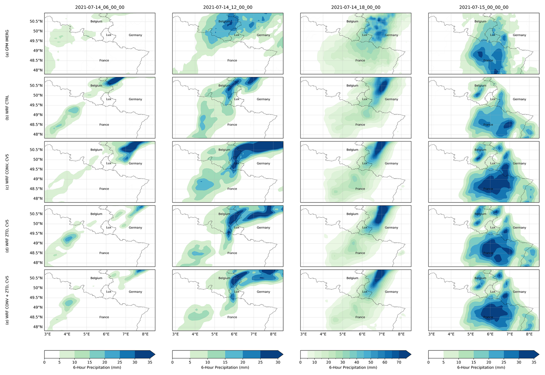
Figure 11 Spatial distribution of 6 h accumulated precipitation (mm) over the Greater Region during 14–15 July 2021, at the indicated UTC times (00:00, 06:00, 12:00, 18:00 UTC). The assimilation rows are the CV5 configurations. Panels: Each field is drawn on its own native grid and no regridding is performed: IMERG on its own latitude–longitude grid and the model on its 12 km grid, with all panels showing 6 h accumulations in mm. The colour scale is set per time step from the satellite maximum, so it differs from that of Fig. 10. (a) GPM IMERG, taken from the IMERG time-averaged product over each 6 h window (a mean rate in mm h⁻¹, multiplied by six) satellite estimates; (b) the no-assimilation control (CTRL); (c) CONV with CV5; (d) ZTD with CV5; (e) CONV + ZTD with CV5. The colour scale maximum is set separately for each time step to the maximum value in the reference field at that time (for example 35 mm at 00:00 UTC and 70 mm at 18:00 UTC) and is applied uniformly across the panels of that time step to facilitate direct comparison. This practice ensures consistency in visualizing potential overestimation or underestimation in the model simulations relative to GPM observations.

The categorical scores, their bootstrap confidence intervals and the absolute-error metrics for precipitation and 2 m temperature are each aggregated over the whole study period and all independent verification stations, and are given with the subsections that discuss them. The main features are summarised below.

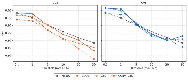
It should be emphasised that the quantitative statistical metrics reported here were computed exclusively against the independent surface-station observations that were withheld from the assimilation; the radar and GPM IMERG datasets were used only for the visual and spatial comparison shown in Figs. 10 and 11 and did not enter the statistical evaluation. The effect of assimilation on categorical skill depends strongly on the intensity threshold, and the full picture is given in Table A1 and Sect. 5.9 rather than summarised by a single threshold here. The outcome is governed by the background error covariance, and the levels behind these differences are shown in Fig. 12. With the climatological CV3 option the model is made to rain more often without discriminating better: at 0.1 mm per 6 h the probability of detection rises from 0.68 in the control to 0.81 for CONV, but the frequency bias rises from 0.96 to 1.37 and the false alarm ratio from 0.29 to 0.41, so the equitable threat score falls from 0.383 to 0.337, with a 95 % bootstrap interval $[-\mathrm{0.055},-\mathrm{0.038}]$ that excludes zero. CONV with CV3 is worse than the control at every threshold tested, from 0.1 to 30 mm per 6 h; the other CV3 configurations are mixed, CONV + ZTD with CV3 being significantly better at 1 mm (+0.025). With the NMC-derived CV5 covariance the same observations improve the score while the frequency bias stays near unity: CONV + ZTD gains +0.031 at 0.1 mm and +0.057 at 1 mm per 6 h, and ZTD alone +0.032 and +0.047; all four exclude zero when grid cells are resampled, but only the two at 1 mm survive a bootstrap over whole days (Sect. 5.9). The gain is confined to low and moderate intensities (at 10 mm per 6 h and above no configuration shows a statistically significant improvement), and it is regionally uneven: for CONV + ZTD with CV5 at 1 mm per 6 h it is +0.099 over Belgium (33 stations, 33 cells), +0.089 over Germany (105 stations, 90 cells), +0.029 over France (92 stations, 86 cells) and −0.001 over Luxembourg itself (34 stations, 27 cells). These regional figures are descriptive: no confidence intervals were computed for the individual countries, and the smaller sets would not support them. The changes in mean bias are statistically significant across the verification network for every configuration (paired Wilcoxon signed-rank test over the 234 grid cells, p<0.001; Sect. 4), whereas no configuration improves the absolute-error metrics for precipitation and several degrade them substantially, confirming that the benefit of assimilation lies in categorical detection and bias correction rather than in absolute-error reduction.

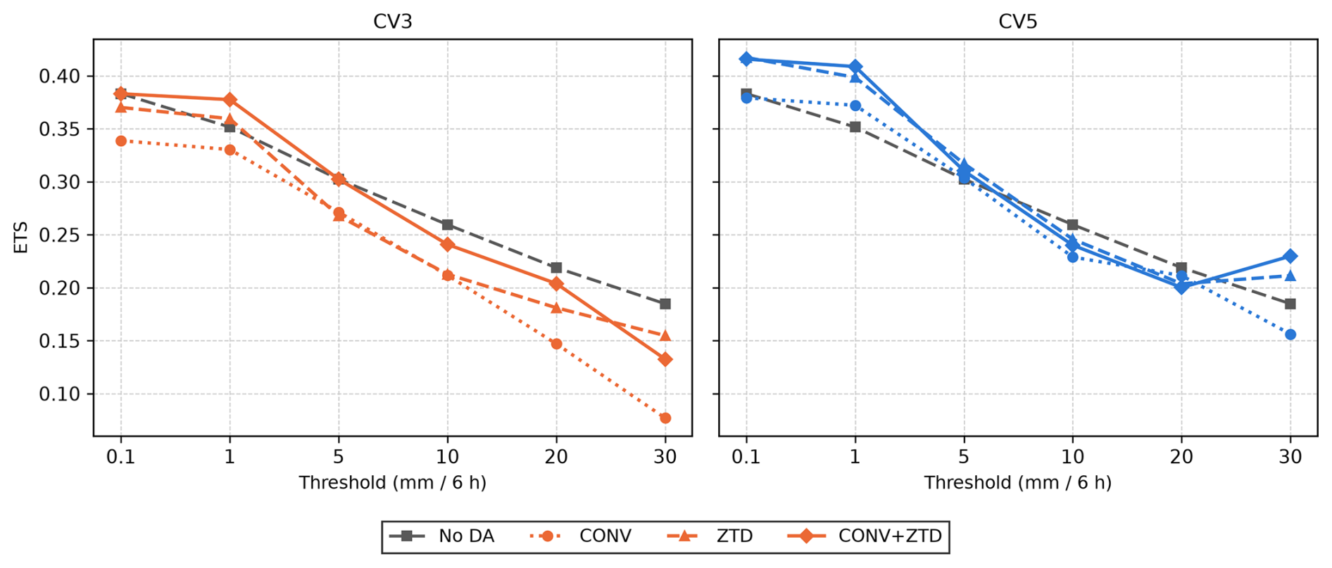
Figure 12 Equitable threat score against precipitation threshold for the climatological CV3 (left) and NMC-derived CV5 (right) background error options, with the no-assimilation control repeated in both panels for reference. Thresholds extend to 30 mm (6 h)⁻¹; above that the number of observed events falls below 150 and the intervals become too wide to interpret.

On the 148-station independent temperature network, every configuration except ZTD with CV3 reduces the cold bias of the control after height correction, while the error magnitude separates the configurations far less: only CONV with CV5 shows a reduction that survives both resampling schemes, and no configuration significantly reduces the root-mean-square error. The statistics and their intervals are given in Sect. 5.6.

The visual comparison is therefore consistent with the categorical scores, and it is the scores rather than the panels that carry the argument.

The absolute-error metrics for precipitation degrade rather than improve: the root-mean-square error rises from 3.63 mm per 6 h for the control to 4.95 mm for CONV with CV3 and 4.21 mm with CV5, and no configuration improves on the control. What assimilation changes is the mean error and the detection of events, not the magnitude of the error.

5.2 Significance of the changes in mean error

The paired test is reported here for the mean error only, and over the 234 model grid cells rather than the 264 stations, so that stations sharing a cell are not counted as independent samples. On that basis the change in mean precipitation error is significant for every configuration (Wilcoxon signed-rank, n=234, $p<{\mathrm{10}}^{-\mathrm{33}}$ in every case), whereas the absolute-error metrics are not improved by any configuration and are significantly degraded by several. Testing the same quantity station by station gives the same verdict for every configuration, so the conclusion does not rest on the choice of unit. Categorical skill is deliberately not tested this way; those differences are assessed with the resampling procedures of Sect. 5.9, which respect the same structure.

5.3 Diagnostics in observation space

Table 6 summarises the O−B and O−A departures accumulated over the 122 analysis cycles. Table 7 adds their means, standard deviations and accepted counts, and Fig. 13 resolves them cycle by cycle. The assimilation behaves as intended for every observation type: the analysis fits the observations more closely than the background does, with root-mean-square reductions of 26 %–30 % for SYNOP and radiosonde temperature and 31 %–33 % for radiosonde humidity. Surface humidity is the exception: CV3 reduces the SYNOP specific-humidity departure by 31 % but CV5 by only 10 %, the one field on which the climatological covariance is the better of the two.

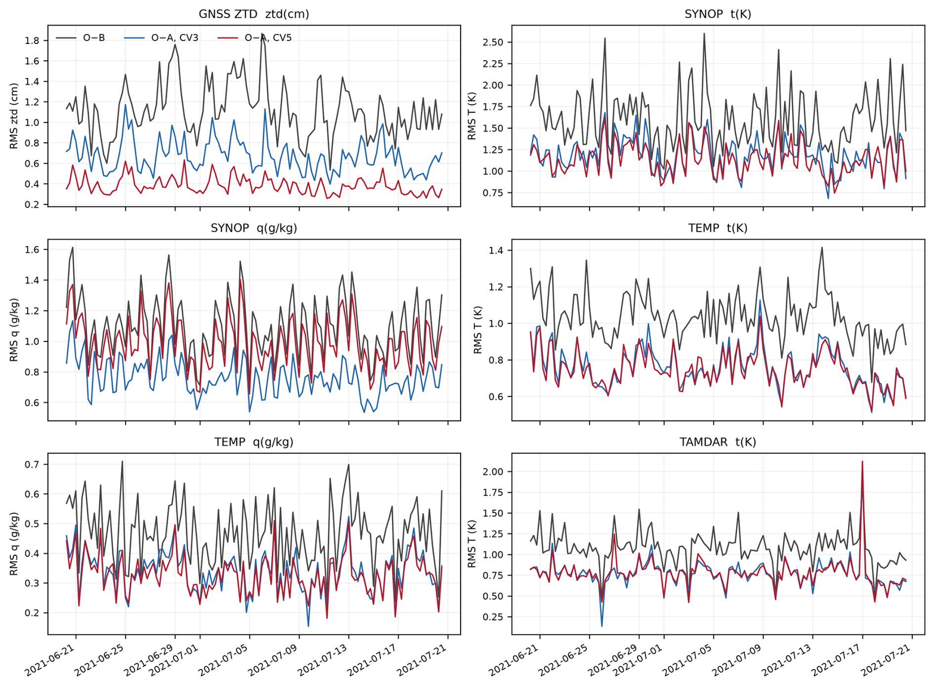
Figure 13 Root-mean-square departure from the background (O−B) and from the analysis (O−A) at each of the 122 analysis cycles, for the observation types that carry most of the information. The background is bit-identical between CV3 and CV5, so a single O−B curve applies to both. The GNSS ZTD panel shows the separation that the month-aggregated numbers summarise: the CV5 analysis fits the delays more closely than the CV3 analysis at essentially every cycle. The SYNOP humidity panel shows the one case where CV5 is the worse of the two, consistent with the aggregated reductions of 31 % for CV3 against 10 % for CV5, and with a domain-specific covariance spreading surface moisture information through the column rather than holding it at the surface.

Table 6 Observation-minus-background (O−B) and observation-minus-analysis (O−A) root-mean-square departures, aggregated over the 122 analysis cycles of 20 June–20 July 2021 and weighted by the number of observations in each cycle. CV3 and CV5 share a bit-identical background, so the O−B column applies to both and the difference between the two O−A columns is attributable to the background error covariance alone.

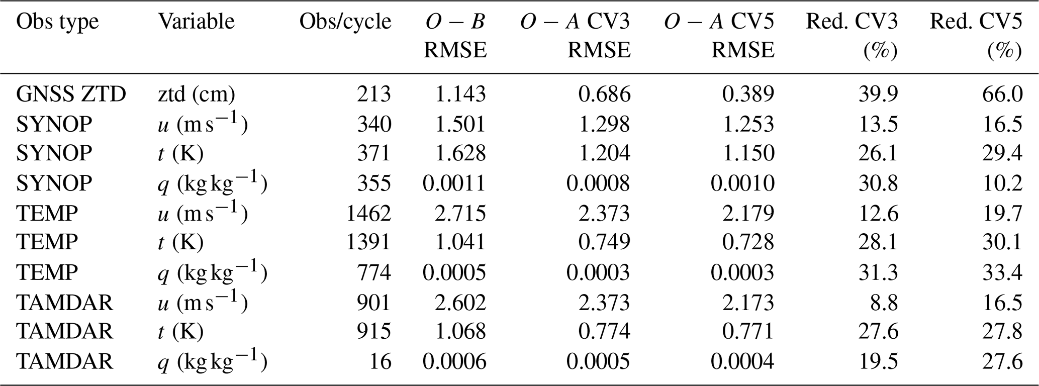
Table 7 Observation-space departure statistics, aggregated over the 122 analysis cycles of 20 June–20 July 2021 and weighted by the number of observations in each cycle. n is the total number of observations accepted by quality control over the month. Mean, RMS and standard deviation are given for the departure from the background (O−B) and from the analysis (O−A); the standard deviation follows from the two moments as $\mathit{\sigma }=\sqrt{{\text{RMS}}^{\mathrm{2}}-{\text{mean}}^{\mathrm{2}}}$. The background is bit-identical between CV3 and CV5, so the O−B columns apply to both. Specific humidity is given in g kg⁻¹.

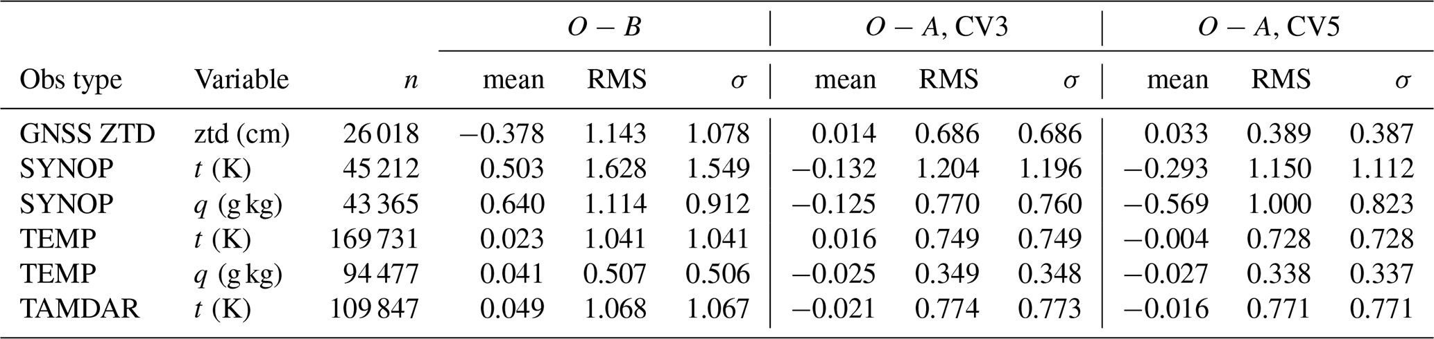
The GNSS ZTD result is the one most directly relevant to the novelty claimed here. An average of 213 ZTD reports per cycle were assimilated after quality control, from 215 available, a rejection rate of 1.0 %. The background departure has a root-mean-square of 1.14 cm and a mean of −0.378 cm, indicating that the background systematically overestimates the delay along the GNSS paths. With the CV3 background error covariance the analysis reduces this to 0.69 cm, a 40 % reduction. With CV5 the same observations and the same background give 0.39 cm, a 66 % reduction. Since the two experiments differ in nothing except the background error covariance, this difference is attributable to B alone. It should not, however, be read as showing that CV5 produces the better analysis, because a closer fit to the observations is not by itself a better fit. With an assigned observation error of 0.8 cm and an O−B root-mean-square of 1.14 cm, the innovations imply a background error of 0.82 cm in observation space, and under a simplified assumption of unbiased and mutually uncorrelated observation and background errors a consistently weighted analysis would leave an O−A root-mean-square of about 0.56 cm. CV3 leaves 0.69 cm and CV5 leaves 0.39 cm, the latter 0.49 of the error assigned to the observations themselves, which on the same assumption corresponds to an effective background error some 37 % larger than the innovations support. These figures suggest that CV3 may draw the analysis less far towards the delays than its own error statistics justify and CV5 further than they support. Because the ZTD departures carry a non-zero mean and the delays are spatially correlated, both assumptions behind the estimate are violated: it is a diagnostic indication rather than a full Desroziers consistency analysis, and it does not establish that the CV5 analysis absorbs observation noise. It is nevertheless the most likely reason that so large a gain in analysis fit yields only a modest, single-threshold gain in forecast skill, and it is consistent with our treating the GNSS ZTD errors as uncorrelated when they are known to be spatially correlated. The comparison still establishes that the covariance governs the outcome; it does not establish that either covariance is correctly tuned, and the diagnostic suggests neither is.

5.4 Categorical skill across thresholds

Table A1 reports the categorical scores at six thresholds for the independent network. At the 0.1 mm threshold POD and FAR alone are misleading. POD rises from 0.68 (No DA) to 0.81 (CONV with CV3), but FAR rises from 0.29 to 0.41 and the frequency bias from 0.96 to 1.37. The equitable threat score, which adjusts for the hits expected by chance, falls from 0.383 to 0.337. The same holds for the other CV3 configurations, whose scores stay at or below the control (ETS 0.368 for ZTD and 0.381 for CONV + ZTD). With CV5 the sign reverses: the equitable threat score rises to 0.416 for ZTD and 0.414 for CONV + ZTD. At the drizzle threshold, therefore, an apparent improvement in detection can be nothing more than the model raining more often, and whether assimilation helps or harms is decided by the background error covariance rather than by the observations.

At higher thresholds the frequency bias improves but the skill does not follow. At 5 mm per 6 h the control rains too rarely, with a frequency bias of 0.66, and assimilation moves it towards unity: 0.94 for CONV + ZTD with CV3 and 0.86 with CV5. The equitable threat score nevertheless barely moves, from 0.302 for the control to 0.302 for CONV + ZTD with CV3 and 0.310 with CV5, while CONV alone with CV3 degrades it to 0.271. At 10 mm per 6 h every configuration is worse than the control (0.259); the closest are ZTD with CV5 (0.246) and CONV + ZTD with CV3 (0.241). Correcting the frequency bias at these intensities therefore does not translate into better discrimination. The benefit of assimilation in this experiment is confined to the low and moderate thresholds, and is not found at the heavy intensities that matter most for flooding.

Figure 14 shows the same scores as a performance diagram, in which the probability of detection is plotted against the success ratio with the critical success index shaded and the frequency bias drawn as rays. It separates the two ways a forecast can gain detection. At the two lowest thresholds every CV3 configuration lies up and to the left of the control (detection rises, the success ratio falls), and CONV with CV3 sits furthest along that path, on a frequency-bias ray of 1.37 at 0.1 mm and 1.46 at 1 mm per 6 h, which is the signature of forecasting rain more often rather than better. The pattern is not uniform across the diagram: at the heavier thresholds several CV3 configurations fall below unit bias, and CONV with CV3 at 30 mm per 6 h loses detection as well as success ratio. With CV5 the points move towards the upper right while staying nearer the unit-bias ray, and the critical success index rises at the two lower thresholds, from 0.443 to 0.473 for CONV and from 0.474 to 0.500 for CONV + ZTD at 1 mm per 6 h. At 5 mm per 6 h and above the points of both covariances lie below the control regardless of bias.

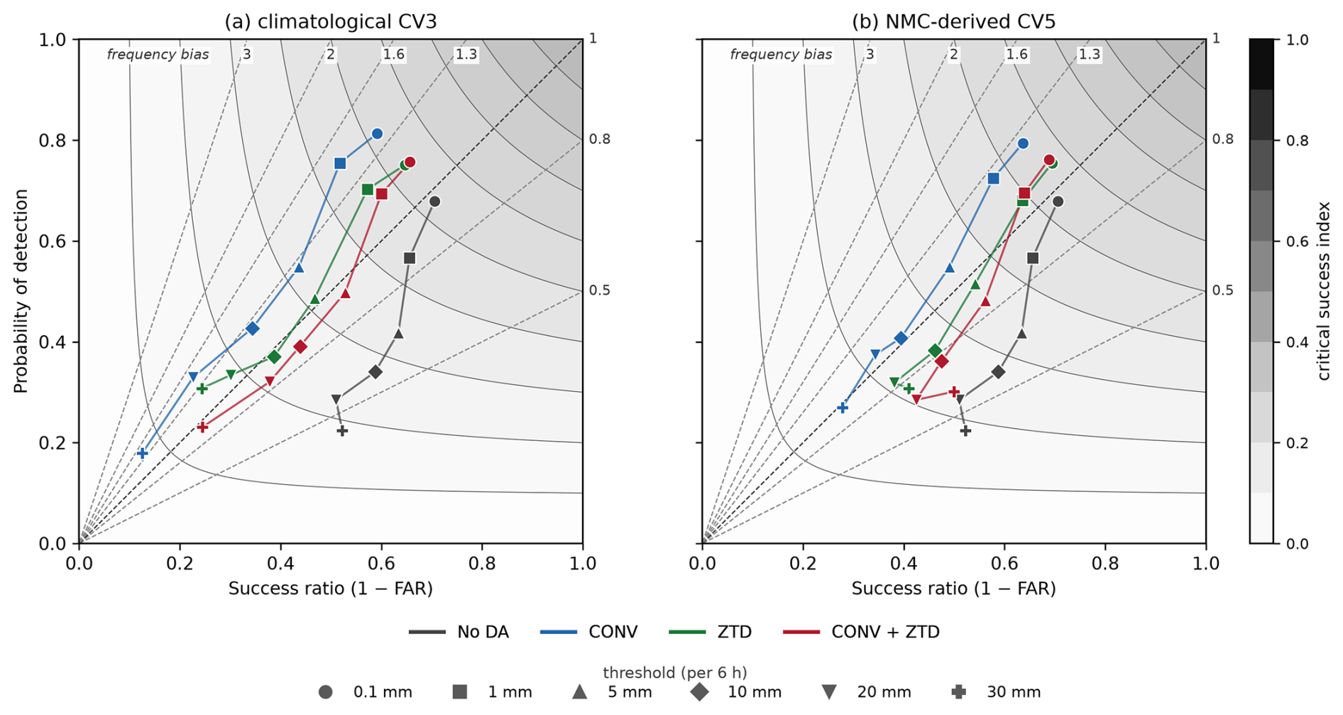
Figure 14 Performance diagram for the 264-station verification network. The probability of detection (POD) is plotted against the success ratio ($\text{SR}=\mathrm{1}-\text{FAR}$). Curved shading and contours are the critical success index, read from the colour bar. The straight dashed rays through the origin are lines of constant frequency bias ($\text{FBI}=\text{POD}/\text{SR}$); the numbers along the top and right edges give the value of that bias for each ray, from 0.5 for a model that rains too rarely to 3 for one that rains three times too often, with the unit-bias ray drawn in black. A perfect forecast lies in the top-right corner. Marker shape denotes the threshold and colour the configuration, with the no-assimilation control repeated in both panels: (a) the climatological CV3 covariance, (b) the NMC-derived CV5. Movement towards the upper right is a genuine gain in skill, whereas movement along a ray away from the origin, or onto a ray of higher bias, is only an increase in how often rain is forecast.

5.5 Sensitivity to the background error covariance

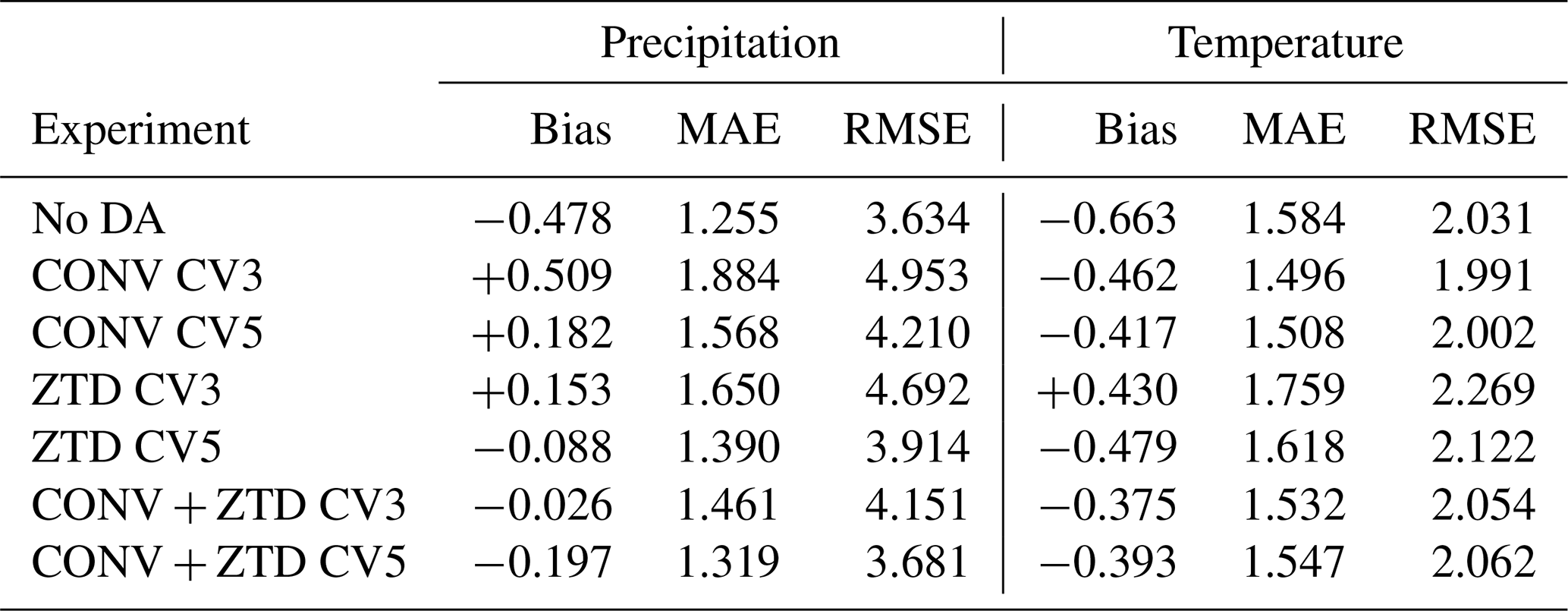
The CV5 configurations improve on their CV3 counterparts in observation space by a wide margin, as described above. In the station verification the advantage is real but much smaller. It is clearest in the false alarm ratio, which each CV5 experiment generally lowers relative to its corresponding CV3 experiment, and in the frequency bias, which the CV5 configurations hold near unity where CV3 inflates it. Against the control the equitable threat score improves only at the two lowest thresholds, and only the gains at 1 mm per 6 h survive both resampling schemes (Sect. 5.9); the direct CV5-against-CV3 comparison, which is a different question, reaches significance at more thresholds than that and is reported in Sect. 5.9 as well. It is not visible at all in the absolute-error metrics: no configuration of either covariance improves the precipitation root-mean-square error on the independent stations, the control value of 3.63 mm per 6 h being the lowest in Table 8, and the closest any configuration comes is 3.68 mm for CONV + ZTD with CV5. The contrast between a 66 % improvement in analysis fit and a forecast improvement confined to one threshold is itself the informative result. Part of it is explained by the consistency check of Sect. 5.3, which shows that the CV5 analysis is drawn inside the assigned observation error, and the remainder is taken up in Sect. 6.

Table 8 Absolute-error metrics on the independent networks. Left: precipitation on all 264 stations (31 760 pairs per configuration). Right: 2 m temperature on the 148 of those stations that report it (34 in Luxembourg, 22 in Germany and 92 in France; 17 774 pairs), with model output adjusted to station height using a 6.5 K km⁻¹ lapse rate. Bias, MAE and RMSE are in mm per 6 h for precipitation and K for temperature. Assimilation moves the mean error towards zero for both variables. For precipitation the error magnitude is larger than the control in every configuration; for temperature the configurations that include conventional observations reduce it, and ZTD alone does not.

5.6 Station and model heights, and their effect on the temperature statistics

Near-surface temperature is verified on the subset of the network that reports it. Of the 264 stations, 148 supply 2 m temperature: all 34 in Luxembourg, 22 of the 105 in Germany (the remaining 83 being precipitation-only gauges that measure no temperature) and all 92 in France. The Belgian gauges are operated by a hydrometric service and report precipitation and discharge only. Every one of the 148 has passed the same independence screening as the precipitation network, the closest lying 12.5 km from any assimilated SYNOP position, and all seven configurations are compared over the same 121 six-hourly times, 17 774 pairs each.

Model terrain and station height differ, and the difference must be removed before the comparison means anything. Model terrain is taken from the WRF HGT field at the same grid point from which the station value is extracted; station heights come from the agrometeorological station list in Luxembourg, the DWD station description file in Germany and the ALTI field of the hourly records in France. Across the 148 stations the model terrain lies on average 14.9 m above the station, with a median difference of 14.6 m and a standard deviation of 63.3 m; 55 stations differ by more than 50 m and 17 by more than 100 m, the extremes being +238 and −183 m. Ninety-one of the 148 lie below the model surface, following the documented tendency for stations to be sited in valleys that a 12 km grid cannot resolve.

Applying the 6.5 K km⁻¹ correction shifts every experiment by the same +0.10 K and leaves the error magnitudes almost unchanged, so it does not reorder the configurations; it matters because it removes a systematic offset that would otherwise be attributed to the assimilation. The corrected statistics are given in Table 8.

Every configuration reduces the cold bias of the control, from −0.66 K to between −0.38 and −0.48 K, the exception being ZTD with CV3, which overshoots to +0.43 K. As point estimates the error magnitude separates the configurations, though the intervals below show that most of that separation is not significant. Assimilating conventional observations lowers the mean absolute error from 1.58 K in the control to 1.50 K with CV3 and 1.51 K with CV5, and the root-mean-square error from 2.03 to 1.99 and 2.00 K. The combined configuration lowers the mean absolute error to 1.53 and 1.55 K while leaving the root-mean-square error slightly above the control at 2.05 and 2.06 K. ZTD alone lowers neither: 1.62 and 2.12 K with CV5, and 1.76 and 2.27 K with CV3.

These differences were tested with the same two resampling schemes used for the categorical scores, resampling the 134 grid cells the 148 stations occupy and, separately, the 31 calendar days. The change in bias is significant under both schemes for every configuration. The change in error magnitude mostly is not. Only CONV with CV5 shows a mean-absolute-error reduction that survives both schemes (−0.077 K, day-block interval $[-\mathrm{0.148},-\mathrm{0.003}]$); the reduction by CONV with CV3 is significant when cells are resampled but not when days are ($[-\mathrm{0.189},+\mathrm{0.014}]$), and no configuration significantly reduces the root-mean-square error. Three degradations are significant under both schemes, all from ZTD assimilated alone: with CV3 it raises the mean absolute error by +0.175 K and the root-mean-square error by +0.238 K, and with CV5 it raises the root-mean-square error by +0.092 K.

The pattern is physically what one would expect. The conventional network includes SYNOP surface temperature reports, so a configuration that assimilates them has direct information about the near-surface state, whereas zenith total delay is a column-integrated moisture quantity whose influence on the 2 m diagnostic is indirect. But the evidence supports a weaker statement than the point estimates alone would suggest: what is established is that every configuration moves the bias towards zero except ZTD with CV3, that the only significant improvement in error magnitude comes from a configuration containing conventional observations, and that the only significant degradations come from ZTD assimilated alone. We do not present temperature as a headline result, and we do not claim a best configuration for it.

5.7 Analysis increments

Figure 15 shows the analysis increment, that is the analysis minus its own background, for the cycle valid at 12:00 UTC on 14 July 2021, at the height of the event, and Fig. 16 shows the corresponding increments of each CV5 configuration separately. The CONV + ZTD experiment is shown with the CV3 covariance beside the same experiment with CV5. Because the two share a bit-identical background and identical observations, the difference between the two columns is produced entirely by the background error covariance.

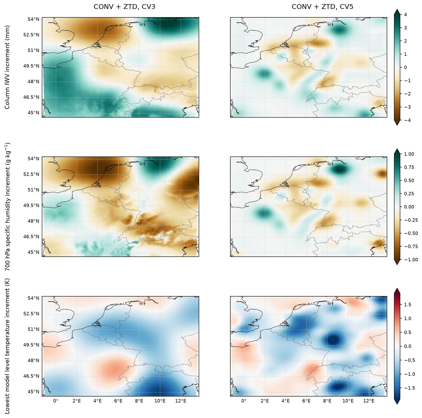
Figure 15 Analysis increment (analysis minus its own background) for the CONV + ZTD configuration at 12:00 UTC on 14 July 2021, with the climatological CV3 covariance (left) and the domain-specific NMC-derived CV5 covariance (right). The two experiments share a bit-identical background and identical observations, so the difference between the columns is produced by the background error covariance alone.

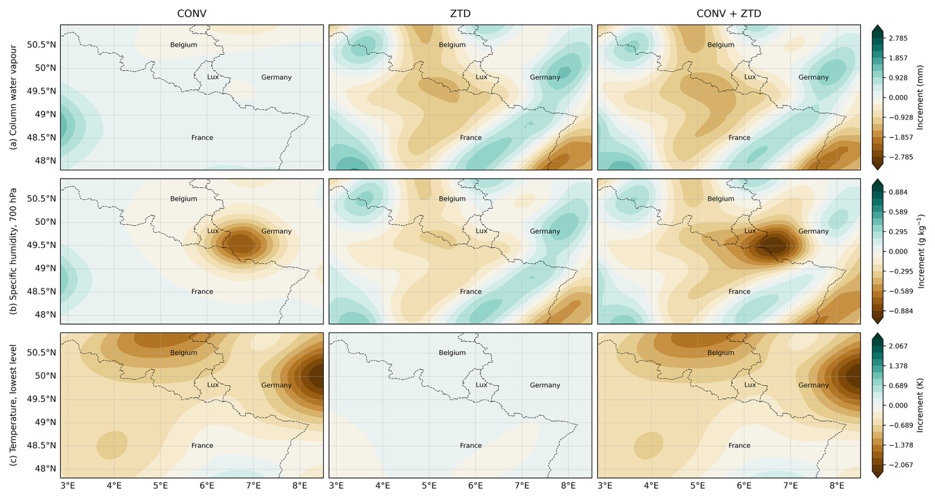
Figure 16 Analysis increments (analysis minus its own background) at 12:00 UTC on 14 July 2021 for the three CV5 configurations, computed from the archived first guess and analysis of each experiment. Rows: column-integrated water vapour, specific humidity near 700 hPa, and temperature at the lowest model level. Root-mean-square increments are given above each panel. CONV and ZTD produce comparable moisture adjustments, 0.52 mm root-mean-square column water vapour for CONV against 0.45 mm for ZTD alone, even though ZTD constrains a single integrated quantity at a few hundred sites while CONV assimilates the full conventional network. The combined configuration produces the largest adjustment (0.68 mm). The 2 m temperature increment is identically zero in every configuration because T2 is a diagnostic field that WRFDA does not rewrite, so the temperature increment is shown at the lowest model level, where CONV and CONV + ZTD adjust the field by 0.60 K and ZTD by 0.01 K. The first guess is byte-identical across the three configurations, as it must be when every cycle starts from the same GFS background.

The contrast is the clearest illustration in this study of why the covariance matters. With CV3 the increments are broad and smooth, spread over distances of several hundred kilometres and bearing little relation to the position of the observations: the column-IWV increment has a root-mean-square of 1.63 mm and coherent features spanning most of the domain. With CV5 the same information is deposited in compact, localised structures concentrated near the observations, with a root-mean-square of 0.67 mm. A climatological, homogeneous and isotropic covariance necessarily spreads a moisture observation over its prescribed correlation length regardless of the meteorological situation, which both dilutes the information and imposes increments where no observation supports them. This is the mechanism behind the difference in analysis fit reported in Sect. 5.3 (40 % against 66 % reduction in ZTD root-mean-square departure).

Two further features of the increments are worth stating explicitly, because they bear directly on how the temperature results should be read. First, the 3D-VAR analysis modifies the three-dimensional atmospheric state (potential temperature, water vapour mixing ratio, the wind components, geopotential and dry surface pressure) but leaves the 2 and 10 m diagnostic fields untouched: the increments in T2, Q2, U10 and V10 are exactly zero in every cycle examined. Second, the soil fields SMOIS and TSLB are also exactly unchanged. Any effect of assimilation on near-surface temperature therefore reaches the 2 m level only indirectly, through the subsequent 6 h model integration responding to the increments aloft, and 3D-VAR does not directly update soil moisture or land-surface temperature, although moisture and cloud increments can alter the surface energy balance indirectly during the forecast. The increment in the lowest model level temperature, which is analysed, has a root-mean-square of 0.58 K in both configurations, several times the typical difference between experiments in the verified 2 m temperature bias. This is discussed further in Sect. 6.

5.8 Spatial signature of assimilation on near-surface temperature

The station statistics summarise the temperature response but do not show where it acts. Figure 17 shows the 6 h forecast impact of each assimilation experiment on the 2 m temperature field at 12:00 UTC on 14 July 2021, that is the difference between the forecast started from the analysis and the forecast started from the background at the same valid time.

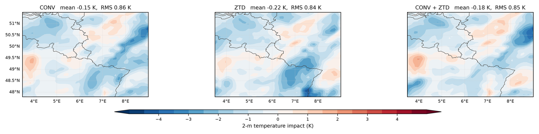
Figure 17 Impact of assimilation on the 2 m temperature field at 12:00 UTC on 14 July 2021, shown as experiment minus no assimilation for the three CV5 configurations. All three produce a slight net cooling of very similar magnitude and none is distinctly larger or more coherent than the others, which is the spatial counterpart of the station result: after height correction the differences between configurations are small.

The impacts are an order of magnitude larger locally than the month-aggregated bias differences of Sect. 5.6: the root-mean-square impact is 0.86 K for CONV, 0.84 K for ZTD and 0.85 K for CONV + ZTD, with local values reaching 5 K. All three configurations produce a slight net cooling over the domain, −0.15 K for CONV, −0.22 K for ZTD and −0.18 K for CONV + ZTD. The three do not share a single moisture explanation: the domain-mean column water vapour increment is +0.22 mm for CONV and +0.07 mm for CONV + ZTD but −0.10 mm for ZTD, so added moisture increasing cloud and reducing daytime heating cannot account for all three, and the cooling is reported as a pattern rather than attributed to one process. The three patterns are of very similar magnitude and no configuration produces a distinctly larger or more coherent signal, which is the spatial counterpart of the station result: the differences between configurations are small once model output is corrected to station height. The figure is therefore the spatial signature of assimilation on the near-surface temperature field rather than evidence for a preferred experiment.

That these large local impacts translate into month-aggregated bias changes of only a few tenths of a kelvin reflects two things: the impacts largely cancel in the spatial and temporal mean, and the verification network samples only a small part of the domain. It is a further reason for reading the small differences between experiments in Sect. 5.6 with caution.

5.9 Confidence intervals for the categorical scores

The categorical verification below covers all seven configurations, as do the absolute-error and temperature statistics of Table 8; the maps of Sect. 5.7 and 5.8 show selected configurations and are labelled accordingly. The conclusions of this paper rest on the categorical results.

Figure 18 and Table 9 give the change in equitable threat score relative to the no-assimilation control, with 95 % intervals from a paired bootstrap over the 234 model grid cells (Sect. 2.4); a second bootstrap resampling whole calendar days is reported below as a check on the temporal dependence the first one ignores. All intervals reported here are pointwise: each is computed for a single configuration at a single threshold, and none is adjusted for the number of comparisons made. The principal result at 1 mm per 6 h is nevertheless supported by surviving both the grid-cell and the whole-day resampling schemes. The outcome divides sharply by background error covariance and by threshold.

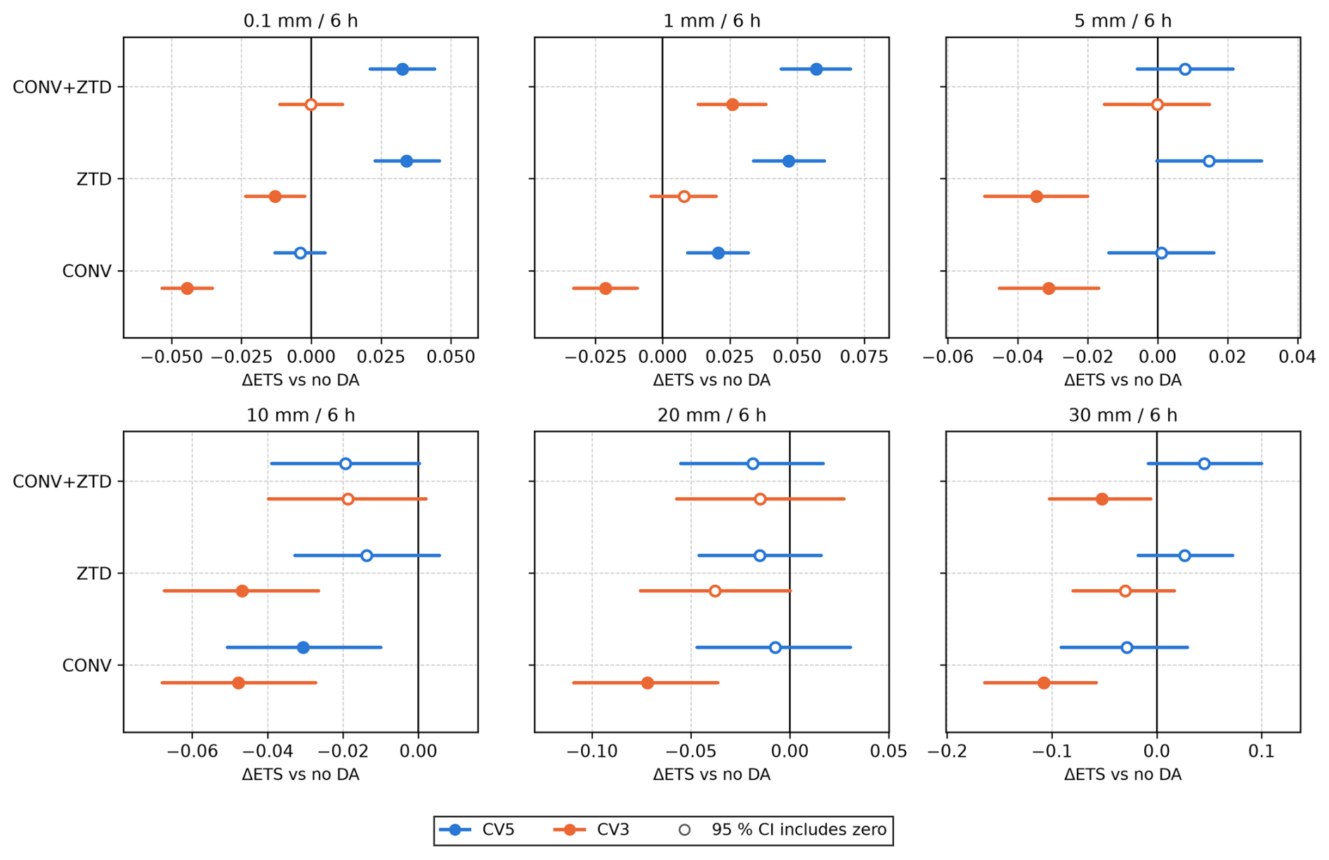
Figure 18 Change in equitable threat score against the no-assimilation control for each configuration and threshold, verified against the 264 independent stations in 234 model grid cells over 121 six-hourly forecasts. Bars are 95 % confidence intervals from 10 000 bootstrap replicates in which grid cells, not stations, are resampled with replacement, because stations sharing a 12 km cell are handed the same model value. Filled markers indicate intervals that exclude zero. The CV3 and CV5 experiments are otherwise identical, so the separation between the two colours is the effect of the background error covariance alone.

Table 9 Change in equitable threat score relative to the no-assimilation control, with 95 % confidence intervals from two paired bootstraps (B=10⁴ replicates each). In the first the resampling unit is the model grid cell, not the station: the 264 stations occupy 234 distinct 12 km cells, and stations inside one cell are handed the same model value, so resampling stations would treat duplicated model values as new information. The second resamples whole calendar days (31 blocks), the conservative test for the temporal persistence of rainfall between cycles.

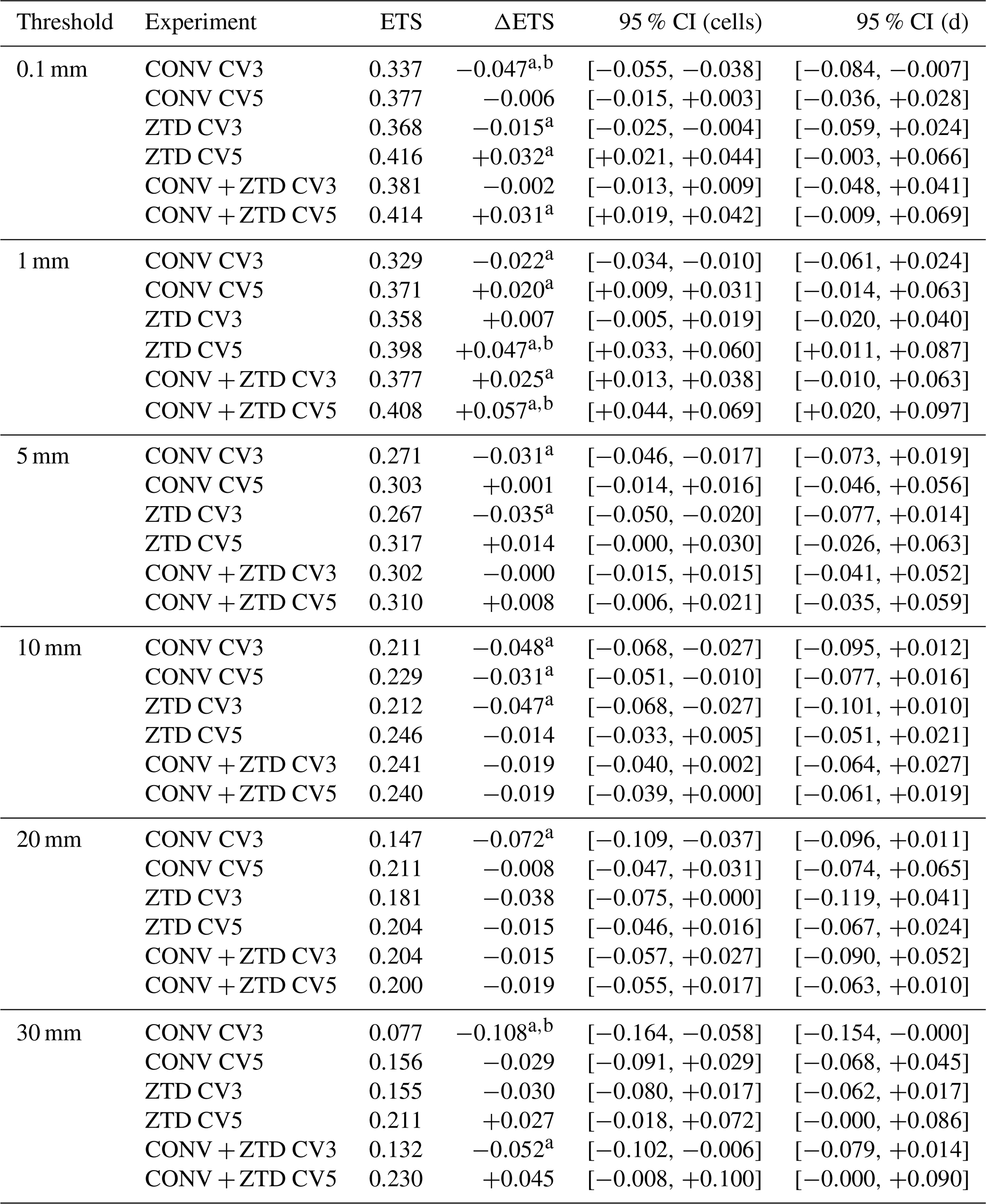
A difference whose interval excludes zero is marked ^a for the cell bootstrap and ^b for the day-block bootstrap; conclusions in the text rest only on differences carrying both marks.

With the climatological CV3 covariance, CONV degrades categorical skill at every threshold tested: −0.047 at 0.1 mm per 6 h (95 % CI $[-\mathrm{0.055},-\mathrm{0.038}]$), −0.022 at 1 mm, −0.031 at 5 mm, −0.048 at 10 mm, −0.072 at 20 mm and −0.108 at 30 mm, every interval excluding zero. The other CV3 configurations are mixed rather than uniformly harmful: ZTD with CV3 degrades the score at 0.1 mm (−0.015) and at 5 mm, while CONV + ZTD with CV3 is significantly better than the control at 1 mm (+0.025, CI $[+\mathrm{0.013},+\mathrm{0.038}]$).

With the NMC-derived CV5 covariance the same observations improve the score at the two lower thresholds. ZTD gains +0.032 at 0.1 mm and +0.047 at 1 mm; CONV + ZTD gains +0.031 and +0.057; CONV alone gains +0.020 at 1 mm. All of these exclude zero.

Two further checks bear on the composition of the network rather than on the resampling. The first concerns proximity to the assimilated GNSS sites. Of the 264 stations, 96 lie within one grid length of a site whose zenith total delay is assimilated: 24 of the 34 in Luxembourg, 50 of the 105 in Germany and 22 of the 92 in France, and none of the 33 in Belgium, which were screened on that criterion (Sect. 2.4). Repeating the whole categorical verification on the 168 stations that clear 12 km from every assimilated GNSS site, in 156 grid cells and 20 210 pairs per configuration, changes no conclusion: at 1 mm per 6 h the CV5 gains are +0.051 for ZTD (95 % interval $[+\mathrm{0.036},+\mathrm{0.066}]$) and +0.059 for CONV + ZTD ($[+\mathrm{0.043},+\mathrm{0.075}]$), slightly larger than on the full network rather than smaller, and no comparison anywhere in the table moves by more than 0.033. Proximity to a GNSS receiver is therefore not a source of dependence for a rain gauge, as expected when the assimilated quantity is a column-integrated delay and the verifying quantity is a surface accumulation.

The cell bootstrap accounts for the dependence between stations sharing a grid cell, but it treats the 121 verification times as fixed, and precipitation persists from one six-hour window to the next. The comparison was therefore repeated with the resampling unit changed from the grid cell to the calendar day, drawing the 31 d of the study period with replacement so that each day carries all of its cells and times. This is a considerably more demanding test, reducing the effective sample from 234 cells to 31 blocks, and only the largest effects survive it: 4 of the 36 comparisons remain significant, against 17 under cell resampling, and the two schemes agree on 23 of 36. What survives is the result the paper rests on. At 1 mm per 6 h the CV5 gains remain significant under both schemes, +0.047 for ZTD (day-block CI $[+\mathrm{0.011},+\mathrm{0.087}]$) and +0.057 for CONV + ZTD ($[+\mathrm{0.020},+\mathrm{0.097}]$), as does the degradation from CONV with CV3 at 0.1 mm ($[-\mathrm{0.084},-\mathrm{0.007}]$) and at 30 mm ($[-\mathrm{0.154},-\mathrm{0.000}]$). What does not survive is the gain at 0.1 mm per 6 h, where the day-block intervals for ZTD and CONV + ZTD with CV5 ($[-\mathrm{0.003},+\mathrm{0.066}]$ and $[-\mathrm{0.009},+\mathrm{0.069}]$) include zero. We therefore rest the positive conclusion on the 1 mm threshold, where both schemes agree, and treat the 0.1 mm gains as suggestive rather than established.

At the flood-relevant thresholds no configuration shows a statistically significant improvement. At 5 mm per 6 h the largest point estimate is +0.014 for ZTD with CV5, whose interval $[-\mathrm{0.000},+\mathrm{0.030}]$ just includes zero. At 10 and 20 mm no positive difference approaches significance, while several degradations do under cell resampling: CONV, ZTD, and CONV + ZTD with CV3 and CONV with CV5 at 10 mm, and CONV with CV3 at 20 mm. At 30 mm the point estimates for ZTD and CONV + ZTD with CV5 are positive (+0.027 and +0.045) but their intervals include zero, whereas the degradation from CONV with CV3 (−0.108) is significant under both schemes. The reason is sample size: the network records 10 030 observed events above 0.1 mm but only 2980 above 5 mm, 1416 above 10 mm and 156 above 30 mm, so the power to detect a difference falls exactly where the meteorological interest is greatest.

The categorical result is therefore threshold-dependent and covariance-dependent. Assimilation with a climatological covariance increases the frequency of forecast rain without improving discrimination, and CONV with CV3 degrades skill throughout. With a domain-specific covariance the combined configuration improves skill at 1 mm per 6 h under both resampling schemes. At the intensities that matter most for flooding no positive difference survives either resampling scheme, so we claim no improvement there; degradation, by contrast, is demonstrable, CONV with CV3 losing −0.108 in equitable threat score at 30 mm per 6 h under both schemes.

Every comparison so far shares the no-assimilation control as its baseline, which settles whether a configuration beats doing nothing but not whether one configuration beats another. Two intervals that both exclude zero, or that overlap each other, say nothing directly about the difference between the configurations they describe. That difference has to be resampled in its own right, and Table B1 in Appendix B does so for the three comparisons the paper's conclusions depend on.

The covariance contrast survives the direct test. With the same observations, CV5 beats CV3 under both resampling schemes at 0.1, 1, 5, and 10 mm per 6 h for ZTD alone, at 0.1, 1, 5, and 30 mm for CONV, and at 0.1 and 1 mm for the combination; the gains are between +0.03–+0.05 at the lower thresholds. The contrast is not uniform: at 5 mm per 6 h it is significant for CONV (+0.032) and for ZTD (+0.049) but not for the combination (+0.008), and at 20 mm no configuration reaches significance. This is the paper's central claim tested directly rather than inferred, and it holds.

The observation contrast is more surprising. Adding GNSS ZTD to the conventional network improves the score significantly under both schemes: +0.037 at 0.1 mm per 6 h (day-block interval $[+\mathrm{0.012},+\mathrm{0.063}]$) and +0.037 at 1 mm ($[+\mathrm{0.009},+\mathrm{0.065}]$). Adding the conventional network to ZTD does not: no threshold shows a difference significant under both schemes, the largest being +0.010 at 1 mm, which survives cell resampling but not day blocks. On this evidence ZTD alone with CV5 is not distinguishable from the combined configuration, and it is the ZTD observations rather than the conventional ones that carry the improvement. We therefore do not present CONV + ZTD as the preferred configuration on the strength of its slightly larger point estimate; what the data support is that ZTD is the component adding skill, and that the covariance matters more than either.

6 Discussion

6.1 Comparison with previous GNSS ZTD assimilation studies

The impact of ZTD assimilation found here is smaller than that reported in several of the studies that motivated this work, and the differences are instructive. Torcasio et al. (2023) and Giannaros et al. (2020) both report clear improvements in precipitation fields from ZTD assimilation, the former over Italy and the latter over Greece from more than 48 stations of the Hellenic GNSS network across seven high-impact events of 2018, four in the dry season and three in the wet; Poletti et al. (2019) report improved rainfall fields in the first six hours over northern Italy by combining radar nowcasting with numerical forecasts rather than by assimilating zenith delays, and Vladimirov et al. (2020) report improved mesoscale precipitation for a winter cyclone over Bulgaria from conventional observations, satellite atmospheric-motion vectors and GNSS radio-occultation refractivity. The last two are therefore not directly comparable ground-based ZTD experiments, and are cited here only for the broader context of moisture-related assimilation.

Torcasio et al. (2023) assimilated zenith total delays from 388 GNSS receivers into WRF over Italy at 3 km grid spacing and verified against more than 3000 rain gauges over a full month, 2–31 October 2019, reporting frequency-bias and probability-of-detection gains that are significant up to 30 mm (3 h)⁻¹ and equitable threat scores that improve significantly at 1, 25, and 30 mm (3 h)⁻¹, against a false alarm ratio whose increase is itself significant up to 20 mm (3 h)⁻¹. Their experiment resembles ours in a way that is easy to miss: they too find that assimilation raises the number of false alarms, and they state explicitly that this limits the improvement in equitable threat score. The parallel is closer than the headline numbers suggest: their equitable threat score also reaches significance at their lowest tested threshold, 1 mm (3 h)⁻¹, which is where our own gain sits. The difference is that theirs survives the rise in false alarms at the intense thresholds as well and ours does not above 1 mm per 6 h, for reasons set out below. Their thresholds are also not ours: 25–30 mm in 3 h is a more intense event than 30 mm in 6 h. We therefore read the two studies as qualitatively consistent (a domain-specific covariance helps, and false alarms are the limiting factor in both) without treating the numbers as equivalent, and we do not set an absolute change in equitable threat score against a percentage improvement, since the two are not the same quantity.

Giannaros et al. (2020) report improvements over Greece that are larger than ours and that extend to intense rainfall: for accumulations above 20 mm they find the probability of detection higher by 10.6 % in the dry season and 3.9 % in the wet, the false alarm ratio lower by 7.7 % and 16.9 %, and the equitable threat score higher by 11.4 % and 8.1 %, all statistically significant. The contrast with our CV3 experiments is instructive, since there the false alarm ratio rises rather than falls. The improvements in equitable threat score obtained here with CV5, between +0.03–+0.06 at 0.1 and 1 mm (6 h)⁻¹, are of the same order as the few-percent ETS gains reported in that literature, so the present results are neither anomalously large nor negligible. Five differences plausibly account for the weaker signal obtained here.

First, the verification samples differ. Several of those studies report skill for selected episodes, whereas every number here is aggregated over a month of 6-hourly cycles that includes long quiescent periods, so a strong impact during the flood episode is averaged with many cycles in which the assimilation has little to correct. Where a study reports both, the event-selected figures are the ones that invite comparison with our flood-period figures, and the month-aggregated ones with our headline numbers.

Second, the observing networks and resolutions differ substantially. The Italian experiment described above resolves convection on its 3 km grid rather than parameterizing it, assimilates a far denser receiver network and verifies on 3-h accumulations, so both the information supplied to the analysis and the sampling of the verification are richer than anything available over the Greater Region, where the assimilated GNSS network is sparse and verification rests on 264 point gauges with 6 h accumulations. Its gauge network, two orders of magnitude larger than one confined to a single country, is also the practical reason the multinational network of Sect. 2.4 was needed before differences of this size could be resolved at all.

Third, and most importantly for the present result, those studies use case-specific, ensemble-based or domain-specific background error covariances rather than a global climatology. Both of the closest comparisons do so explicitly: Torcasio et al. (2023) generated theirs with GEN_BE by the NMC method using the CV5 option, and Giannaros et al. (2020) derive theirs for their domain by the NMC method from differences between 24–12 h forecasts for five control variables, the construction tested here as CV5. That both studies obtained clear improvements with a domain-specific covariance, while our CV3 configurations degrade the score and our CV5 configurations improve it, is consistent rather than contradictory: it is the same result seen from two directions. Half of the configurations here use the climatological CV3 option, and the comparison shows directly how much that costs: with identical observations and an identical background, changing only B improves the ZTD analysis fit from a 40 % to a 66 % reduction in root-mean-square departure. A climatological, homogeneous and isotropic covariance cannot spread a moisture increment along the anisotropic structures of a convective moisture field, and much of the information in the ZTD observations is therefore discarded at the analysis step. The domain-specific covariance improves on this by representing the average forecast-error variances, length scales and inter-variable relationships of this domain; it remains static, and cannot represent the event-specific structure of the moisture field either.

The choice of background error covariance has not been settled in this literature. The WRFDA guidance itself states that it is difficult to say in advance which option performs better and that the impact varies from case to case, and published comparisons are mostly of CV5 against CV6 rather than against CV3. The result reported here, that with the conventional observations CV3 not only underperforms CV5 but is worse than no assimilation at every threshold tested, because it inflates the frequency bias from 0.96 to 1.37 at 0.1 mm and 1.46 at 1 mm per 6 h, is therefore a specific contribution to an open question rather than a confirmation of an established one.

Fourth, the design used here re-anchors the background to the GFS analysis at every cycle (Sect. 3.2). Increments do not compound from one cycle to the next, so the month-long experiment is not equivalent to a month of continuously accumulating assimilation. This is a deliberate choice that keeps the experiments comparable and prevents drift, but it necessarily limits the achievable impact.

Fifth, the verification metric matters. Several of the cited studies emphasise spatial agreement of rainfall fields, whereas the quantitative results here rest on point-gauge comparisons, which are the least forgiving measure available for a convective event.

Thundathil et al. (2024) extended WRFDA with an observation operator for tropospheric gradients, and Thundathil et al. (2025) showed that adding gradients to zenith delays from a sparse network produces an improvement comparable to assimilating zenith delays alone from a network of twice the density. Since the present study assimilates zenith delays only, that finding indicates a concrete route to further improvement over this domain that does not require additional receivers, and it is identified as the natural next step in Sect. 7.

6.2 Factors limiting the impact of assimilation

Four features of this experiment bound what assimilation can deliver, and they should be borne in mind when comparing the numbers reported here with other studies.

First, the GFS analyses that provide the initial and boundary conditions have already assimilated most of the SYNOP, radiosonde and aircraft observations that the CONV experiment ingests. The conventional increment is therefore largely a re-assimilation of information the background already contains, which is consistent with the modest CONV impact found here and with the observation that CONV mainly increases the frequency of forecast rain rather than improving its placement. GNSS ZTD is the one observation type in this study that is not already in the GFS analysis at comparable density, which is an argument for the ZTD component rather than against it. Second, the 12 km grid with the Grell–Freitas cumulus parameterization (Table 5) cannot represent the convective cells that produced the extreme local rainfall of 14–15 July 2021. Convection is parameterized, so the model produces rainfall of approximately the right areal extent but cannot reproduce the intensity peaks recorded at individual gauges. This interacts with the double-penalty problem: when a parameterized convective cell is displaced by even one or two grid lengths from the observed cell, verification against point gauges counts both a miss and a false alarm, so a forecast that improves the position of a rainfall feature can score worse than one that produces broad, weak, ubiquitous rain. The rise in frequency bias and fall in ETS at the 0.1 mm threshold reported in Sect. 5.4 is consistent with this limitation, although the categorical scores alone cannot isolate displacement error as its cause. It does not, however, mean that the signal is clearer at the heavier thresholds. At 5 mm per 6 h no configuration improves significantly on the control, and at 10 mm every configuration scores below it: the double penalty is harder to satisfy with widespread drizzle there, but the sample of observed events is also far smaller, and the model's inability to place a parameterized convective cell tells against it more strongly.

Third, two aspects of how the GNSS delays were handled work against the high-threshold result. The delays were assimilated without thinning and without statistical bias correction. WRFDA's conventional-observation thinning controls, which can act on zenith delays, were not activated in these experiments, and its variational bias correction is implemented for satellite radiances. Applying a statistical correction to zenith delays therefore requires treatment outside the assimilation system, as in Torcasio et al. (2023). On average 213.3 of the roughly 215 available ZTD reports were assimilated in each cycle, whereas 150 of the 234 sites lie within 20 km of another site and 27 within 5 km; a thinning mesh that had culled those neighbours would have left far fewer reports. Receivers that close sample much the same air, so their errors are correlated, while R treats them as independent, and that is the mechanism behind the over-weighting identified in Sect. 5.3, where the CV5 analysis fits the delays to about half their assigned error. The background departure likewise retains a mean of −0.378 cm throughout the month (−0.404 cm over the first half and −0.352 cm over the second, with no trend), which is 47 % of the assigned observation error and 35 % of the innovation spread; a bias correction acting on these observations would have driven that mean towards zero, although the mean itself cannot be attributed to the observations or to the background with the information available here, since separating observation bias from model bias requires an independent reference (Dee, 2005). Variational bias correction of the kind implemented here (Auligné et al., 2007) is formulated for satellite radiances, so centres that assimilate ground-based ZTD estimate station-dependent corrections from observation-minus-background statistics instead (Poli et al., 2007; Bennitt and Jupp, 2012), and Torcasio et al. (2023) likewise subtract each receiver's mean observation-minus-background departure before assimilating it, retaining one receiver per model grid cell so that no pair is closer than about 10 km. Applying such a correction here is left to future work.

Neither point is likely to matter much at the drizzle threshold, where the signal is large and the sample is 10 030 events, but both bear on the intense thresholds, where the sample is 156 events above 30 mm per 6 h and the control produces such events only 43 % as often as they are observed. A model that cannot generate the peak has little for the assimilation to correct, and a network whose information content is over-counted supplies increments that are noisier than their number suggests. We therefore regard the absence of a high-threshold signal here as a property of this configuration rather than as evidence that GNSS ZTD cannot help at those intensities, and we identify thinning that actually reaches the delays, a bias correction applicable to them, and a covariance whose weights the innovations support, as the changes most likely to alter it.

Fourth, the pathway from a ZTD increment to a near-surface temperature response is indirect. 3D-VAR updates the atmospheric state only, with either covariance; soil moisture and soil temperature are not analysed and are carried from the GFS-derived land state. A moisture increment can influence 2 m temperature through the radiative effect of altered column humidity and cloud, and through modified boundary-layer mixing, but it cannot act through a direct update of the surface energy balance, which is the dominant control on the diurnal temperature cycle. This is a further reason for treating the small temperature differences between experiments in Sect. 5.6 with caution, and it motivates the recommendation to couple moisture assimilation with land-surface initialisation in future work.

6.3 Limitations

The principal limitations of this study follow from the points above: a single 12 km domain with parameterized convection; a climatological background error covariance for half of the configurations, whose cost is quantified by the direct CV3–CV5 comparison; an analysis that is re-anchored to GFS at every cycle and therefore does not accumulate; a verification network of 264 independent stations in 234 grid cells, which remains modest for stratifying by intensity at the highest thresholds; and the absence of any land-surface analysis. The GNSS network used here is also sparser than the Italian and Greek networks of the studies with which we compare, and its delays reached the analysis neither thinned nor bias-corrected (Sect. 6); the thinning controls that would act on them were not activated and no statistical bias correction was applied, of the kind used operationally (Poli et al., 2007; Bennitt and Jupp, 2012).

Two further limitations bear directly on how the results should be read. The first is that the CV5 covariance was generated from forecast differences over 21 June–19 July 2021, a window that overlaps the period evaluated here. The CV3–CV5 comparison is therefore an in-sample sensitivity test: it establishes that the formulation of the background error covariance changes the result, and by how much, but not the skill an operationally independent covariance would deliver. Generating one from an independent period is identified in Sect. 7 as the immediate next step. The second is the scope of the temperature comparison. It rests on 148 of the 264 stations: all 34 in Luxembourg, all 92 in France and 22 of the 105 in Germany, the remaining 83 German sites being precipitation-only gauges that measure no temperature. No Belgian station contributes, because the Service Public de Wallonie gauges are operated for hydrometry and report precipitation and discharge rather than air temperature, so the temperature results carry no information about Belgium, the country over which the precipitation gain was largest.

7 Conclusions and Outlook

This study evaluated the impact of assimilating conventional meteorological observations (CONV) and GNSS Zenith Total Delay (ZTD) data, individually and in combination, into the WRF model using the WRFDA 3D-VAR framework with two background error covariances, the climatological CV3 and an NMC-derived CV5. Seven configurations were run at 6-hourly intervals over the full month of 20 June–20 July 2021 (no assimilation, and CONV, ZTD, and CONV + ZTD with each of the climatological CV3 and NMC-derived CV5 background error covariances), each analysis being initialised from the concurrent GFS analysis rather than from its predecessor, and were verified against 264 surface stations in Luxembourg, Belgium, Germany and France confirmed to be independent of the assimilation and occupying 234 distinct model grid cells, with radar and GPM IMERG used for spatial comparison, during the extreme July 2021 flood event in Luxembourg and the Greater Region. Returning to the questions posed in the Introduction, the following conclusions can be drawn.

First, the effect of assimilation on precipitation depends on the background error covariance, while for near-surface temperature the benefit comes from the conventional observations rather than from GNSS ZTD. For precipitation the result is governed by the background error covariance rather than by the observation type. With the climatological CV3 option the assimilation makes the model rain more often without discriminating better: at 0.1 mm per 6 h CONV raises the probability of detection from 0.68 to 0.81 but raises the frequency bias from 0.96 to 1.37 and the false alarm ratio from 0.29 to 0.41, and the equitable threat score falls significantly from 0.383 to 0.337 (95 % CI on the difference $[-\mathrm{0.055},-\mathrm{0.038}]$). CONV with CV3 is worse than no assimilation at every threshold tested, up to 30 mm per 6 h, while the other CV3 configurations are mixed. With the NMC-derived CV5 covariance the same observations improve the score, CONV + ZTD gaining +0.031 at 0.1 mm and +0.057 at 1 mm per 6 h with the frequency bias held near unity. Only the gain at 1 mm survives a bootstrap over whole days, so that is the threshold on which the positive result rests. Two limits on that gain should be stated plainly. It is confined to low and moderate intensities: at and above 10 mm per 6 h no configuration improves significantly on the control (the point estimates at 30 mm are positive for the two CV5 configurations but their intervals include zero), so no improvement is claimed at the intensities most relevant to flooding. And it is regionally uneven: the improvement is largest over Belgium and Germany, smaller over France, and absent over Luxembourg itself, where no configuration improves categorical skill at the lower thresholds. For 2 m temperature, verified on the 148 stations that report it, every configuration reduces the cold bias of the control, from −0.66 K to between −0.38 and −0.48 K, except ZTD with CV3, which overshoots to +0.43 K. The error magnitude separates them less clearly. Only CONV with CV5 shows a reduction in mean absolute error that survives both resampling schemes (−0.077 K), no configuration significantly reduces the root-mean-square error, and the three significant degradations all come from ZTD assimilated alone. The differences are small against a root-mean-square error of about 2 K, and we identify no best configuration for temperature. Second, the two observation types are not interchangeable, and which one matters depends on the variable. In particular the assimilation of GNSS ZTD cannot be credited with the near-surface temperature response: once model output is corrected to station height, the configurations that improve it are those containing conventional observations, and ZTD assimilated alone improves neither the mean absolute nor the root-mean-square error. For precipitation with CV5, the combined configuration cannot be distinguished from ZTD alone: tested directly against each other, the largest positive difference in favour of CONV + ZTD is +0.018 at 30 mm per 6 h and +0.010 at 1 mm, and no threshold produces a difference significant under both resampling schemes (Table B1). The reverse comparison is decisive: adding ZTD to the conventional network gains +0.037 at both 0.1 and 1 mm per 6 h, significant under both schemes. For precipitation, therefore, it is the GNSS observations that carry the improvement and the conventional observations add nothing detectable once ZTD is present, while for near-surface temperature the position is reversed. Third, and the clearest result of this study, the representation of background error matters more than the choice between these observation types. Tested directly, CV5 beats CV3 with the same observations under both resampling schemes at 0.1 and 1 mm per 6 h for all three observation sets, and at 5 mm for CONV and for ZTD alone though not for the combination, by between +0.03–+0.05 in equitable threat score (Table B1), a margin comparable in size to the gain from adding ZTD but far more consistent across thresholds and observation sets. This contrast is established in-sample, the CV5 covariance having been derived from a window that overlaps the evaluation period, and it therefore bounds the size of the effect rather than the skill an operationally independent covariance would deliver. Fourth, and notably, even though the GNSS moisture signal constrains only a spatially limited portion of the atmosphere, its assimilation produced a measurable impact when assessed over a full month of repeated six-hourly cold-start assimilation and forecast experiments, though one confined to a single threshold and to part of the domain. The value of ZTD assimilation for this region lies in improved low-threshold rain-occurrence detection and in the mean precipitation bias rather than in the reduction of absolute error magnitude. Indeed, no configuration improves the absolute-error metrics for precipitation and several degrade them substantially (the root-mean-square error rises from 3.63 mm per 6 h for the control to 4.95 mm for CONV with CV3), indicating that what assimilation changes is where and whether rainfall is forecast, not how much.

Taken together, these findings show that a modest, moisture-focused observation such as ZTD can improve the detection of rainfall occurrence in the Greater Region, provided the background error covariance is derived for the domain. They do not show a benefit at flood-producing intensities: at and above 10 mm per 6 h no configuration improves significantly on the control, and the improvement that does exist is absent over Luxembourg itself. The distinction between detecting that it will rain and predicting how much matters for this application, and on the present evidence only the first is improved.

Several avenues remain for future work. The covariance is the single most promising place to work next, but the analysis-fit numbers overstate what is available there: the consistency check of Sect. 5.3 shows that CV3 draws the analysis less far towards the ZTD observations than the innovations justify while CV5 draws it further, fitting them to about half their assigned error. What is needed is therefore not simply a more finely tuned covariance but one whose implied weights the innovation statistics support, generated from a period independent of the evaluation and combined with an observation error that reflects the spatial correlation of GNSS ZTD rather than treating the delays as independent. Diagnosing that correlation, thinning the network to a spacing that reflects it, estimating station-dependent corrections on a training period independent of the evaluation and testing them on the remainder, and scaling the background error variances accordingly, together form the immediate next step. Beyond this, four directions follow from the limitations identified in Sect. 6: running at convection-permitting resolution so that the intensity of convective rainfall is represented rather than parameterized; cycling hourly rather than 6-hourly, and allowing the analysis to propagate between cycles so that increments accumulate; assimilating additional GNSS products such as slant delays or tropospheric tomography, which carry directional information that ZTD alone does not; and initialising soil moisture, since the temperature results point to a surface-layer pathway that 3D-VAR of atmospheric variables cannot reach. Expanding the validation network and integrating real-time GNSS ZTD streams would further improve the detection reliability required for operational flood forecasting in the Greater Region.

Appendix A: Categorical verification scores at all six thresholds

Table A1 lists the frequency bias, probability of detection, false alarm ratio, critical success index and equitable threat score for every configuration at each of the six thresholds. The behaviour it records is described in Sect. 5.4 and shown in Figs. 12 and 14; the table is given here in full so that the individual counts behind those figures can be checked.

Table A1 Categorical verification scores in full, against the 264 independent stations (234 model grid cells, 121 six-hourly forecasts, 31 760 forecast–observation pairs per configuration). FBI is the frequency bias, POD the probability of detection, FAR the false alarm ratio, CSI the critical success index and ETS the equitable threat score. The CV3 and CV5 columns differ only in the background error covariance.

Appendix B: Configuration-against-configuration comparisons

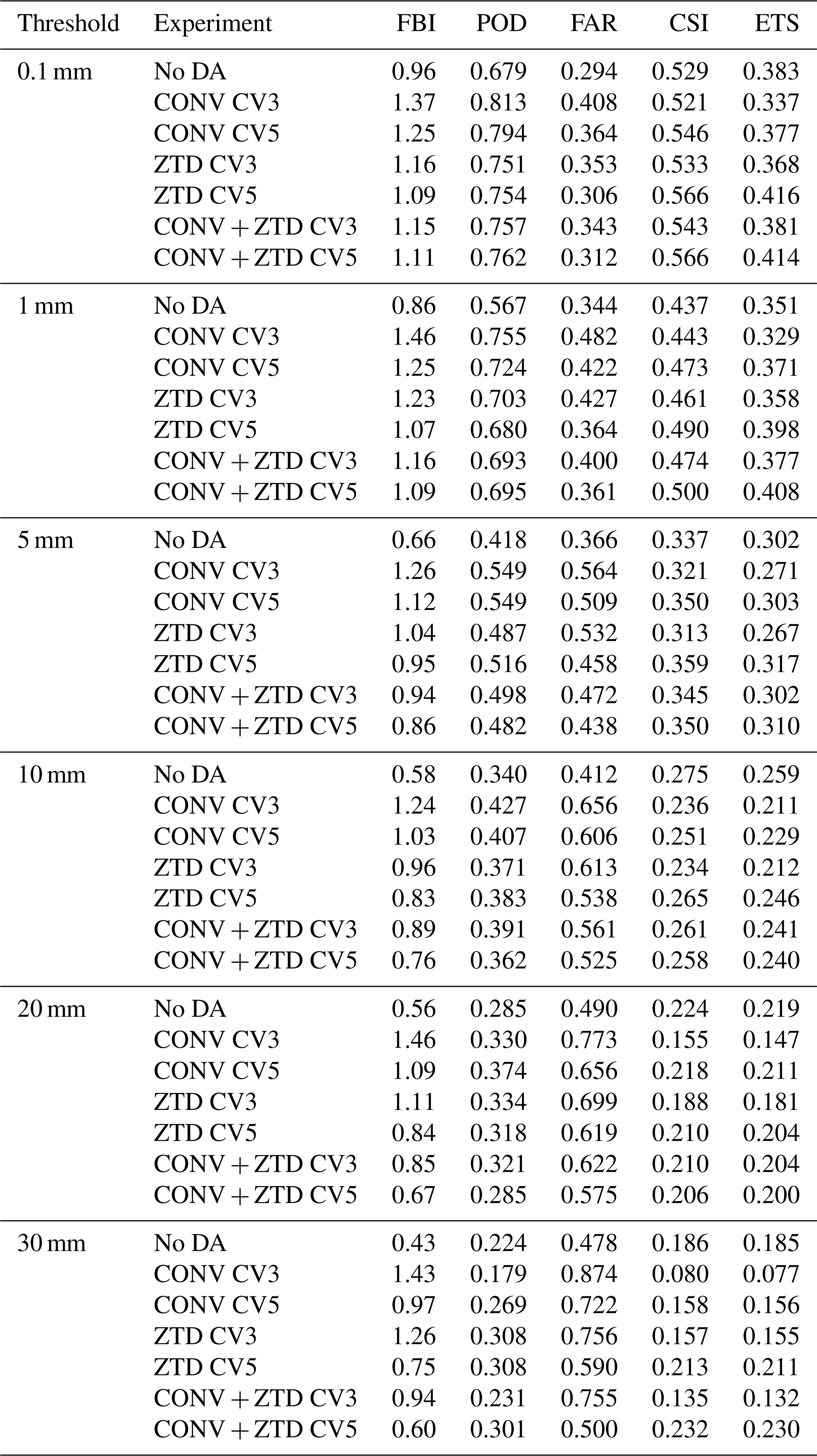
Table B1 gives the differences between configurations discussed in Sect. 5.9, at every threshold and under both resampling schemes. They are collected here because each entry is a separate paired bootstrap and the table is long; the comparisons the conclusions rest on are quoted in the text.

Table B1 Differences in equitable threat score between configurations, rather than between a configuration and the control. Each row resamples the difference itself, paired, with 95 % intervals from the grid-cell and the day-block bootstrap (B=10⁴ each). These comparisons cannot be read off Table 9, in which every entry shares the no-assimilation control as its baseline. Positive values favour the first configuration named.

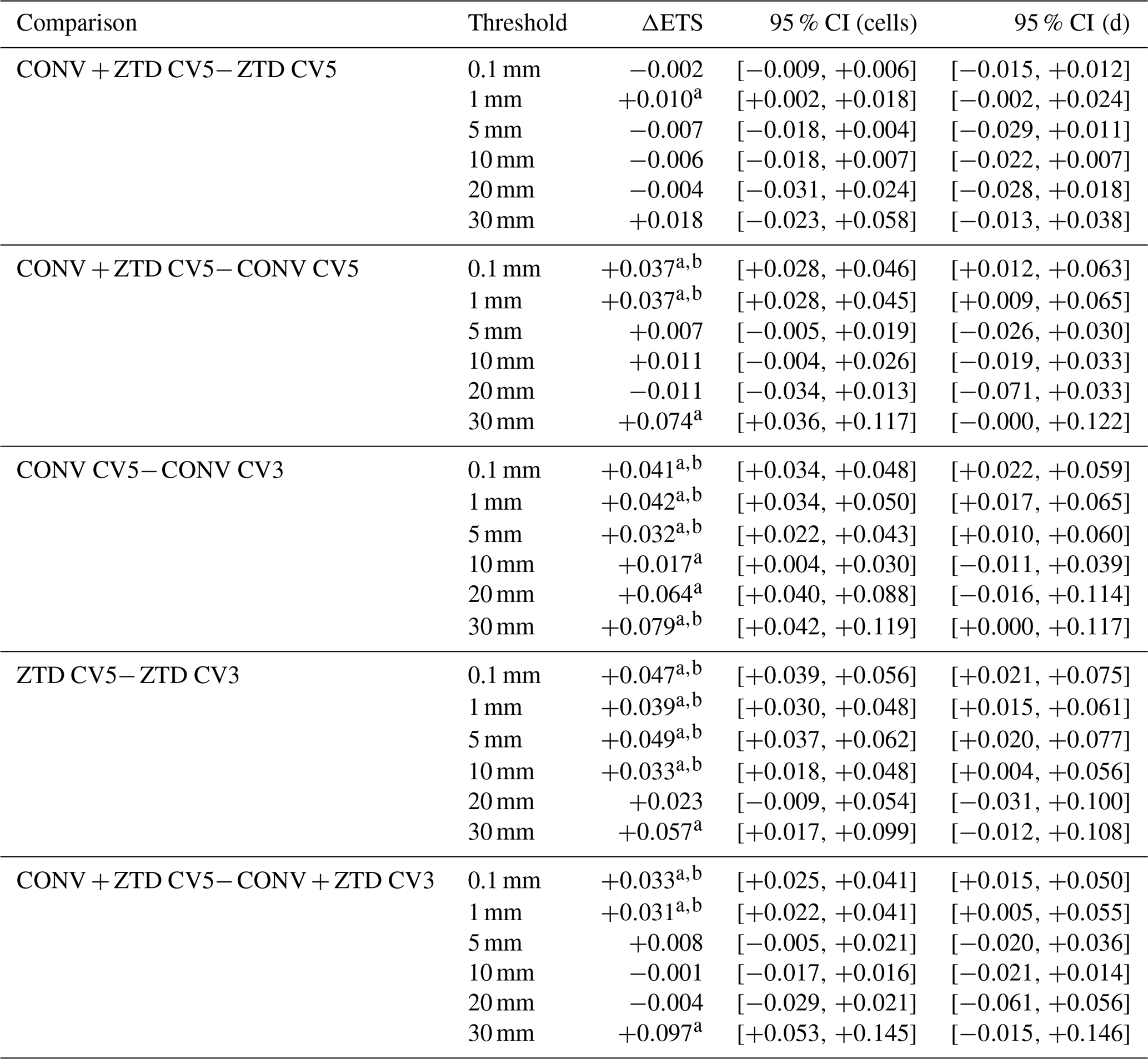
A difference whose interval excludes zero is marked ^a for cells and ^b for days.