Flood exposure and structure damage under deterministic design-storm and stochastic storm transposition rainfall scenarios: a case study in South Louisiana, USA

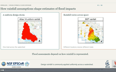
Flood hazard maps and damage estimates guide floodplain management, mitigation planning, and engineering design, but they commonly rely on rainfall frequency analysis to define annual exceedance probability (AEP) storms, commonly referred to as design storms. Current engineering practice typically employs spatially uniform design storms derived from point-based gauge statistics; however, this approach suppresses the spatial organization and intensity gradients present in observed storms. Stochastic storm transposition (SST) offers an alternative by preserving the spatial structure of observed rainfall and stochastically repositioning full storm fields across a watershed. This study compares flood exposure and damage produced by Atlas 14 and SST rainfall representations in the Vermilion River Basin, a low-gradient inland–coastal watershed in south-central Louisiana. Although the TP40-adjusted Atlas 14 rainfall depth was larger than the mean basin-average SST accumulation across the 50 realizations (310 mm vs. 238.1 mm), the SST_max composite produced substantially greater total structure damage than the baseline Atlas 14 scenario (USD 0.923 billion vs. USD 0.477 billion). Moreover, the comparison identified 11 518 buildings that were inundated in at least one SST realization but not under Atlas 14, representing more than USD 110 million in cumulative structural damage. The divergence between the two approaches is concentrated in mid-elevation urban neighborhoods, where spatial rainfall variability can cross local inundation thresholds that were not crossed under the spatially uniform storm. These results show that, in the VRB, the spatially uniform Atlas 14 design storm missed localized flood exposure that emerged when storm placement and rainfall spatial variability were represented.

1 Introduction

Quantitative flood-risk assessments rely on the consistent linkage of flood hazard characterization, exposure, and economic loss estimation. Within this chain, rainfall frequency analysis and the derivation of design discharges are central to estimating flood damage risk, as they determine the exceedance probabilities that underpin hazard maps and expected annual damage curves (Merz et al., 2002, 2008; Büchele et al., 2006; Nofal and van de Lindt, 2022). This study investigates how the choice of annual exceedance probability (AEP) storms, commonly referred to as design storms, affects structure damage estimates in a low-gradient inland-to-coastal (transitional) basin. Typically, direct flood damage is estimated by intersecting inundation maps with representations of the building stock and translating water depths into monetary losses using depth-damage relationships or more detailed vulnerability models (e.g., Dutta et al., 2003; Scawthorn et al., 2006; Schwarz and Maiwald, 2008). Merz et al. (2010) summarize this workflow as a sequence of (i) exposure analysis, which identifies elements at risk and their asset values, (ii) susceptibility analysis, which describes how these elements respond to flooding, and (iii) aggregation of losses across sectors such as private households, services, industry, public infrastructure, and lifelines. They emphasize that, despite the central role of damage estimates in benefit-cost analysis, risk mapping, and insurance pricing, damage data are sparse, methods are often crude, and model formulations are frequently transferred across regions, time periods, and damage processes without sufficient justification. In this study, we focus on improving the methods used for flood risk mapping and structure damage estimation by evaluating how the usual simplifications in defining design rainfall shape the resulting flood maps and the losses inferred from them.

A wide spectrum of approaches is used to model the flood damage estimation workflow from triggering weather events to flood damage. These range from relatively simple combinations of flood frequency analysis with stage-damage curves (e.g., Merz et al., 2002) to fully distributed hydrologic-hydraulic simulations that resolve inundation dynamics and building-scale exposure (e.g., Dutta et al., 2003; Apel et al., 2004, 2008). Merz et al. (2008) frame flood risk as the probability of adverse consequences due to inundation and demonstrate with a case study in Germany that the total uncertainty in risk estimates arises from the superposition of multiple components, including flood frequency, rating-curve uncertainty, and depth-damage relationships. Their Monte Carlo analysis shows that damage estimation dominates uncertainty for relatively frequent events, whereas flood frequency estimates dominate for larger return periods, and that ignoring these uncertainties can materially affect mitigation decisions. Pavesi et al. (2024) and Merz et al. (2008) also highlight a practical tension: detailed hydraulic models are often required for credible inundation mapping, but their computational cost discourages the ensemble simulations needed for rigorous uncertainty analysis, especially over large river reaches. Pavesi et al. (2024) emphasized that although simplifying modeling assumptions leads to easy implementations, enduring a higher computational cost by adopting finer modeling detail can lead to improved flood risk maps.

Recent comparative studies show that exposure and damage estimates are highly sensitive not only to the choice of damage model but also to how flooding exposure is estimated. Gutenson et al. (2023) found that different inundation mapping approaches for Hurricane Harvey in the Clear Creek watershed yielded estimates of 6279–72 601 inundated structures and USD 0.7–3.3 billion in combined structure and content damage. Grimley et al. (2025) showed that transition-zone dynamics during Hurricane Florence, where inland runoff and coastal surge interact, can elevate water levels beyond what would be obtained from purely coastal or purely upland drivers, implying that partial representations of the physical system may underestimate risk in compound settings. These studies, along with broader work on compound flooding (e.g., Moftakhari et al., 2017), highlight the need for damage assessments coupled with flood models that capture the dominant physical mechanisms, rather than simplified or single-driver configurations.

The challenges in flood risk assessment, therefore, extend beyond damage functions or model parameters to the underlying hazard representation. Bodoque et al. (2023) and Merz et al. (2010) note that flood damage assessment has historically lagged flood hazard analysis and that deterministic scenarios are still commonly used in regulatory and engineering practice. In the United States, hazard products and design guidance remain anchored to past conditions, using maps such as the United States Federal Emergency Management Agency (FEMA)'s Special Flood Hazard Areas and point-based intensity-duration-frequency curves like NOAA Atlas 14 (Perica et al., 2013). Wing et al. (2022) show that FEMA's current floodplain maps capture only about 41 % of contemporary flood risk, implying that many exposed structures are systematically missed. The non-stationarity of extreme precipitation documented by Milly et al. (2008) adds to this problem, because biases in how historical storms are represented translate directly into biased estimates of flood losses.

Conventional practice assumes a one-to-one correspondence between rainfall and discharge return periods, using spatially uniform design storms derived from gauge-based statistics and, where needed, depth-area reduction factors such as those in TP40. Studies using stochastic storm transposition (SST) have shown that this assumption can break down because flood response depends not only on rainfall volume, but also on storm organization, basin scale, land-surface properties, antecedent conditions, and the spatial alignment of intense rainfall with watershed structure (Wright et al., 2013, 2014, 2017, 2019; Zhu et al., 2018). RainyDay, introduced by Wright et al. (2017), provides an open-source implementation of SST for generating long records of transposed space-time rainfall fields from gridded precipitation datasets. SST-based flood-frequency studies have demonstrated that spatially uniform, deterministic rainfall representations can misrepresent flood response when storm structure and placement interact with watershed properties (Wright et al., 2014, 2017; Zhu et al., 2018). This issue is closely related to pluvial flooding, where intense local rainfall and limited drainage capacity can produce inundation away from the main river corridor; previous studies have shown that stochastic space-time rainfall methods can be useful for representing such rainfall-driven flood hazards in urban areas (Simões et al., 2015; Mediero et al., 2022). More generally, prior work shows that the relationship between rainfall frequency and flood-response frequency depends on basin scale, storm organization, rainfall space-time structure, land-surface properties, and antecedent conditions. SST provides a physically-based alternative to deterministic, spatially uniform storms by treating historically observed storms as space-time rainfall fields and repositioning them within a homogeneous extreme-rainfall domain, preserving internal intensity gradients and temporal evolution while exploring a wide range of plausible storm placements relative to the drainage network. SST can therefore provide rainfall hazard inputs that retain spatial and temporal storm structure, allowing the effects of storm placement on inundation depth patterns and structure damage estimates to be evaluated explicitly.

Recent SST applications have extended this framework beyond rainfall and discharge frequency analysis toward flood inundation, exposure, and damage estimation. Perez et al. (2024) advanced the process-based flood frequency analysis-SST (FFA-SST) framework by coupling RainyDay-generated synthetic storms with a spatially resolved hydrologic model to estimate frequency curves for peak flow, basin inundation fraction, and population flood exposure. Baer et al. (2026) further demonstrated the implications of spatiotemporal rainfall variability for flood risk by comparing design-storm and SST-based estimates of flood hazard and expected annual damage. These studies highlight the value of SST for evaluating the non-unique relationship between rainfall frequency, inundation, exposure, and losses, while also showing that broader probabilistic SST-to-risk analyses can require large numbers of hydrologic, hydraulic, and damage simulations.

Spatial rainfall representation can be important in hydrologically complex, low-gradient systems such as the Vermilion River Basin (VRB) in south-central Louisiana, where inundation is governed by the timing and spatial alignment of tributary peaks, floodplain storage, and backwater effects from coastal boundary conditions (Awaad et al., 2025; Saad and Habib, 2021; Saad et al., 2021). This study investigates how shifts in storm spatial-temporal representation and placement can change knowledge of both where flooding occurs and the depth of flooding, with direct implications for structure damage estimates and mitigation priorities.

Building on prior SST studies of rainfall–flood frequency relationships and rainfall space-time structure (Wright et al., 2014, 2017; Zhu et al., 2018), and recent extensions of SST toward inundation, exposure, and damage estimation (Perez et al., 2024; Baer et al., 2026), this study addresses a gap at the intersection of rainfall hazard representation, high-resolution hydraulic modeling, and building-level consequence analysis. We evaluate building-level flood exposure and structure damage in the VRB under two contrasting rainfall representations of the 100-year, 24 h event: (1) a deterministic, spatially uniform NOAA Atlas 14 AEP storm, spatially adjusted using Technical Paper 40 (TP40; Hershfield, 1961) depth-area relationships, and (2) an ensemble of 50 SST realizations constructed from gauge-adjusted radar rainfall fields.

We use a calibrated hydrologic-hydrodynamic coupled model developed as part of the Louisiana Watershed Initiative (LWI, 2021) with a detailed representation of channels, floodplain storage, and hydraulic structures to simulate flood inundation depths and extents in the VRB low-gradient inland-coastal watershed. The resulting depth fields are intersected with the National Structure Inventory (NSI; USACE, 2026) and converted to structure economic losses using standardized United States Army Corps of Engineers (USACE) depth-damage functions (USACE, 2003, 2021), allowing assessment of how alternative hazard definitions change inundation extent, depth distributions, exposure, and the distribution of basin-wide damages.

The remainder of this paper is organized as follows. Section 2 introduces the Vermilion River Basin and its hydrologic setting. Section 3 describes the rainfall forcing scenarios, the coupled hydrologic-hydrodynamic modeling framework, and the damage estimation analysis. Section 4 examines how the choice of rainfall representation affects the distribution of inundation depth, estimates of aggregate damages and exposure gaps, and the spatial organization of inundation clusters. Section 5 discusses what the results imply for flood-risk assessment in our study area. Finally, we summarize our main conclusions in Sect. 6.

2 Study Area

The VRB (Fig. 1) is a low-gradient inland-coastal watershed in south-central Louisiana, USA. The basin drains an area of approximately 1500 km² into the Vermilion Bay and the Gulf of Mexico. The Vermilion River collects runoff from a dense network of small tributaries that drain a mix of urban, suburban, and agricultural areas, including the City of Lafayette and surrounding communities (Awaad et al., 2025; Saad and Habib, 2021; Saad et al., 2021). Slopes along the main stem are very mild (average slope of 1 foot for every 10 river miles or 0.0000189 m m⁻¹). As a result, the water levels are controlled by spatial variations in hydraulic head imposed by tributary inflows, wetland storage, and coastal water levels rather than a simple upstream-downstream gradient. During extreme rainfall events, floodwater moves bidirectionally toward parts of the basin that have a lower head. This causes internal division points at some locations where discharge splits in different directions, and where net flow is near zero for extended durations even while the surrounding areas remain inundated (Awaad et al., 2025). The basin contains a total of 173 327 National Structure Inventory (NSI; USACE, 2026) structures of various types (e.g., commercial, residential, industrial, educational, or government).

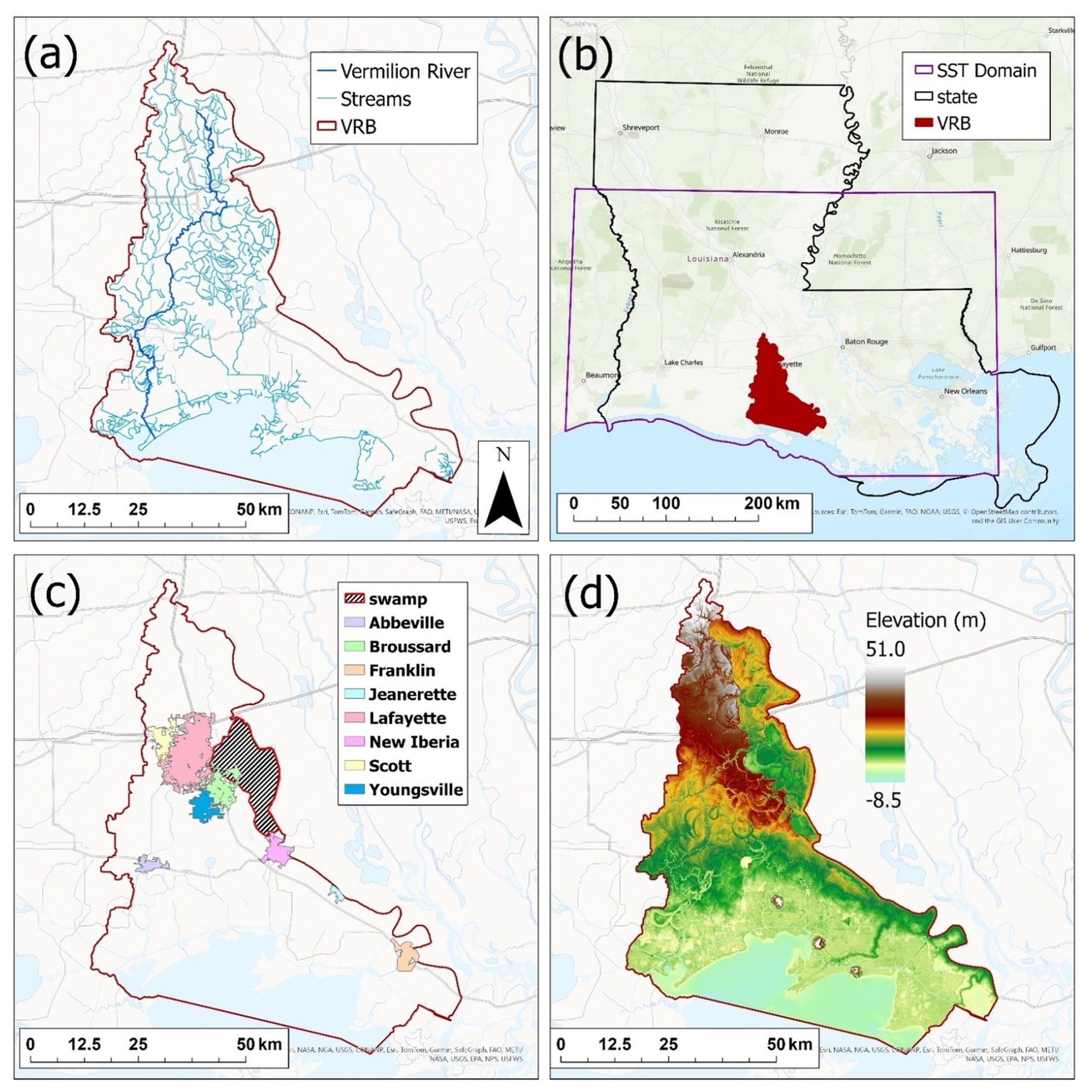
Figure 1 Spatial maps showing the different characteristics of the Vermilion River Basin (VRB). Panel (a) shows the drainage area of the VRB (red line), the main stem of the Vermilion River (dark blue line), and the basin tributaries (light blue). Panel (b) shows the SST domain used in this study (purple polygon) relative to the VRB and the state of Louisiana. Panel (c) shows the population centers in the basin (major cities), as well as the swamp area connected to the Vermilion River. Panel (d) shows the elevation in meters across the basin where low-lying flat areas such as the swamp area and the inland-coastal transition zone are depicted in dark. (Sources: Esri, NASA, NGA, USGS, CONANP, TomTom, Garmin, SafeGraph, FAO, METI, NOAA, EPA, NPS, USFWS, © OpenStreetMap contributors, and the GIS User Community. Map created using ArcGIS^® software by Esri | Powered by Esri).

3 Methods

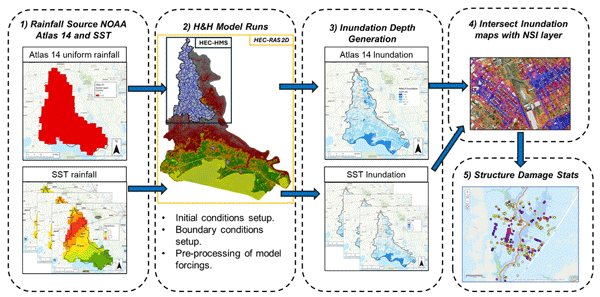
Figure 2 summarizes the overall workflow used in this study. Rainfall inputs are first defined using two alternative 100-year representations, the spatially uniform NOAA Atlas 14 deterministic storm and the spatially variable SST storm realizations, which serve as forcings to the coupled HEC-HMS and HEC-RAS (USACE, 2023) modeling framework. The hydrologic and hydrodynamic models are then run to generate gridded maximum inundation depths for each scenario. These depth rasters are then intersected with the National Structure Inventory (NSI) point layer to determine structure-specific flood depths, which are subsequently translated into structure damages using the depth-damage procedures described in Sect. 3.3.1. The resulting building-scale impacts are finally aggregated to produce basin-wide damage statistics that form the basis for comparing the impacts from the two design storm methods on structure damage assessment.

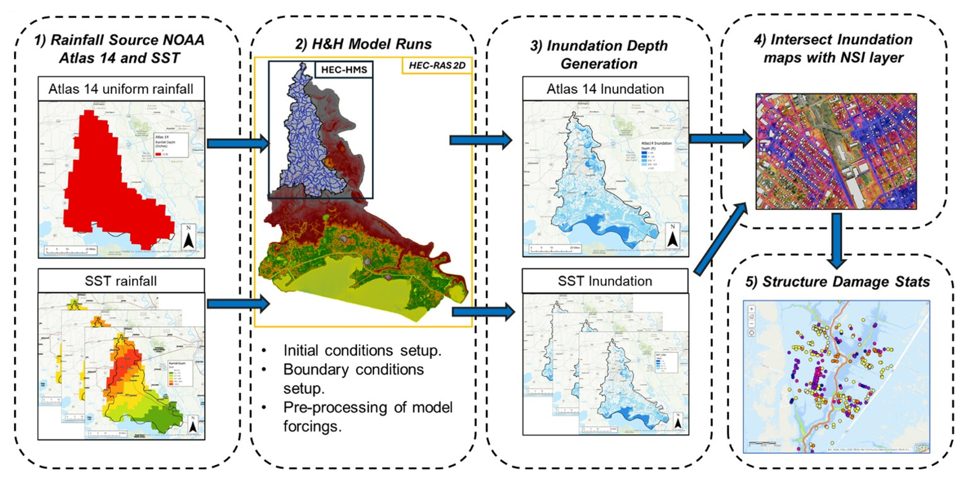
Figure 2 Workflow used to evaluate flood exposure and damage. Step (1) generates the rainfall inputs used to drive the hydrologic and hydrodynamic (H&H) models, including uniform Atlas 14-based rainfall and SST-based rainfall fields. Step (2) defines the H&H model setup, including rainfall pre-processing and specification of model initial and boundary conditions. The 2D HEC-RAS model domain (gold rectangle) covers the entire basin, while the HEC-HMS domain is shown by the black rectangle. Step (3) consists of executing the model simulations and producing SST inundation depth composites. In Step (4), the resulting inundation maps are overlaid with National Structure Inventory (NSI) building locations to calculate inundation depth and inundation frequency at each structure. Step (5) computes the damage statistics described in Sect. 3.3. (Sources: Esri, NASA, NGA, USGS, CONANP, TomTom, Garmin, SafeGraph, FAO, METI, NOAA, EPA, NPS, USFWS, © OpenStreetMap contributors, and the GIS User Community. Map created using ArcGIS^® software by Esri | Powered by Esri).

3.1 Rainfall forcing scenarios

This study compares two distinct representations of the 100-year, 24 h design storm over the VRB. The first is a conventional uniform storm with rainfall depths obtained from NOAA Atlas 14 (Perica et al., 2013). These rainfall depths are derived from point-scale frequency analysis of historical gauge records. Although Atlas 14 is spatially distributed as gridded maps, the underlying values represent point-based depth estimates and require significant approximations to be applied to larger spatial scales (i.e., Area Reduction Factor; ARF). We obtained the 100-year, 24 h depth from the Atlas 14 gridded product near the basin centroid and validated it against nearby rain gauge records. We then applied a depth-area adjustment following Technical Paper 40 (TP40; Hershfield, 1961) to obtain an areal average consistent with the effective basin area. The basin-scale rainfall depth was distributed over 24 h using the alternating-block method, with the peak rainfall block centered at 50 % of the storm duration for the baseline Atlas 14 simulation (Chow et al., 1988; Lee and Ho, 2008). The resulting rainfall hyetograph was then applied as a spatially uniform rainfall field over both the hydrologic and hydrodynamic modeling domains.

To contextualize the baseline Atlas 14 scenario within conventional design-storm uncertainty, we also conducted three additional Atlas 14 sensitivity simulations. First, we simulated the upper bound of the NOAA Atlas 14 90 % confidence interval using the same TP40 depth-area adjustment and 50 % alternating-block temporal pattern as the baseline Atlas 14 case. Second, we evaluated sensitivity to temporal peak placement by repeating the baseline Atlas 14 rainfall depth with the alternating-block peak shifted to 25 % and 75 % of the 24 h storm duration. These additional Atlas 14 simulations were not used to redefine the primary comparison, but they provide a sensitivity check on how rainfall-frequency uncertainty and temporal-pattern assumptions affect exposure and damage estimates under a spatially uniform design-storm framework.

The second rainfall representation was generated using stochastic storm transposition (SST) with RainyDay (Wright et al., 2017) and the NCEP Stage IV gauge-adjusted radar rainfall archive for 2002–2020. SST treats historically observed storms as space-time rainfall fields that can be repositioned within a broader transposition domain assumed to have similar extreme-rainfall characteristics. The SST domain used in this study is shown in Fig. 1b and was selected to include the VRB and surrounding areas with broadly similar rainfall-producing mechanisms, while also being large enough to provide a sufficient catalog of historical parent storms for transposition. We acknowledge that SST domain selection is an important methodological choice because the selected domain determines which historical storms are available for transposition and where they may be repositioned. Historically, SST domains have often been defined using regional and meteorological judgment; however, objective and reproducible methods for domain delineation are an active area of research. For example, FitzGerald et al. (2026) introduced an L-moments-based hypothesis-testing framework for identifying statistically homogeneous storm-transposition regions. Applying and evaluating alternative objective domain-delineation procedures was outside the scope of the present study, which focuses on how the selected rainfall representation affects modeled inundation and structure damage estimates.

Parent storms were identified from the Stage IV record by selecting 24 h rainfall events over the SST domain while enforcing a minimum temporal separation of 24 h between storms. The initial catalog contained 350 24 h parent storms, corresponding to approximately 19 storms per year over the Stage IV archive used in this study. Among the 50 routed 100-year SST realizations used in this analysis, the contributing parent events began on 29 August 2012, 16 October 2006, 12 August 2016, 9 March 2016, 25 October 2015, and 29 August 2017. The extracted storms were then inspected, and 26 events with less-than-optimal radar rainfall quality were excluded before stochastic resampling. Fifty distinct SST realizations were carried forward into the analysis. This realization count was selected to balance stochastic sampling of plausible 100-year storm placements with the computational expense of running the full hydrodynamic and consequence-analysis chain, and it is consistent with prior RainyDay/SST applications using computationally intensive hydrologic models.

The primary model-forcing set therefore consists of the baseline Atlas 14 uniform storm and 50 SST storm realizations. The additional Atlas 14 confidence-bound and temporal-peak simulations were used only as sensitivity cases to contextualize the baseline Atlas 14 comparison.

3.2 Hydrologic and Hydrodynamic Modeling Framework

To evaluate the sensitivity of flood-risk estimates to how the rainfall hazard is defined, a calibrated and verified one-way coupled hydrologic-hydrodynamic modeling framework was employed. The system was originally developed for the Louisiana Watershed Initiative (LWI) Region 5 and covers the VRB HUC-8 domain. The framework couples a semi-distributed hydrologic model (HEC-HMS V 4.11) for the upstream, high-relief portion of the VRB watershed with a two-dimensional hydrodynamic model (HEC-RAS V 6.4.1) for the lower-lying portions of the basin (Figs. 1d and 2 step 2). Outflows from HEC-HMS serve as inflow boundary conditions for HEC-RAS. The rain-on-grid capability in HEC-RAS was used to represent direct rainfall on the floodplain surface. Together, these components optimized runtime and were applied across multiple simulations to characterize flood routing and inundation behavior across the basin.

There is no significant flow contribution from neighboring watersheds, and all connections to the neighboring watersheds have hydraulic control structures. We implemented stage hydrograph time series representing the real conditions at these structures during flood events (e.g., closed gates preventing additional water from entering the basin). The domain was discretized into 187 sub-basins and 146 routing reaches. Runoff losses were represented using the gridded deficit-and-constant loss method, with parameters derived from Soil Survey Geographic Database (SSURGO; Soil Survey Staff, 2026) soils data and adjusted for land development and imperviousness. Excess precipitation was transformed to runoff using the ModClark method (Feldman, 2000) to capture distributed watershed response while maintaining computational efficiency. During calibration, loss and ModClark timing parameters were adjusted to improve runoff volume and hydrograph timing, after which a consistent parameter set was applied across events with event-specific initial deficit values. Baseflow was simulated with the recession method, and channel routing was performed using the Muskingum-Cunge approach (Ponce and Yevjevich, 1978). Calibration and validation were conducted against eight historical flood events, including six calibration events and two validation events covering both tropical and non-tropical storms. The resulting runoff hydrographs were used as boundary inflows to the 2D hydrodynamic model, and performance of the coupled model was evaluated using the stage/WSE and discharge metrics described below, following the Louisiana Watershed Initiative model-performance framework (LWI, 2021).

Floodplain inundation was simulated using HEC-RAS version 6.4.1 with the rain-on-grid configuration. The 2D model domain covers approximately 3626 km², including the Vermilion River main stem and the associated floodplain. An unstructured mesh was used, with characteristic cell sizes of ∼ 90 m in rural areas and 15–30 m in urbanized or hydraulically constrained reaches. The terrain model was constructed from a USGS QL2 (or higher) lidar-based digital elevation model (DEM), supplemented with channel bathymetry from single-beam sonar surveys to maintain cross-sectional integrity and capture backwater-affected low-gradient flows. Spatially distributed Manning's n values were derived from the 2019 NLCD (Dewitz, 2021), with localized adjustments in engineered or vegetated corridors. Calibration regions were applied to refine roughness in stream channels and Vermilion Bay, with adjustments guided by channel width, aerial imagery, and site conditions. During calibration, roughness values were adjusted to improve hydrograph timing and shape, while maintaining physically reasonable ranges. The final calibrated roughness values were fixed for validation events and provided consistent performance across all simulated storms. More than 615 bridges, culverts, and other hydraulic structures were explicitly represented based on detailed survey data. Rainfall was applied through rain-on-grid, and model behavior was confirmed against USGS water-surface elevations and high-water marks from events including Hurricanes Laura (2020) and Delta (2020). Model calibration and validation followed the Louisiana Watershed Initiative (LWI) modeling framework under which the Vermilion regional model was developed and reviewed (LWI, 2021). Model performance was assessed using the Pearson product-moment correlation coefficient (PPCC), standardized root mean square error (RMSE%), and percent bias (PBIAS) for both stage/water-surface elevation (WSE) and discharge. The performance targets were PPCC ≥ 0.9, RMSE% ≤ 15 %, and PBIAS ≤ 10 % for stage/WSE, and PPCC ≥ 0.7, RMSE% ≤ 20 %, and PBIAS ≤ 15 % for discharge. Following the LWI event-level screening criterion, a metric was considered acceptable for an event when at least 50 % of the evaluated gauges met the relevant threshold.

This event-level screening approach was used together with additional model-performance checks because the VRB model represents a large, low-gradient inland–coastal watershed where flood response is influenced by backwater effects, floodplain storage, hydraulic controls, and spatially variable runoff contributions. The available gauge network is unevenly distributed across the basin and includes only two discharge gauges. Model evaluation therefore considered the quantitative event-level statistics together with hydrograph timing, hydrograph shape, peak response, and high-water-mark comparisons where available. Table S1 summarizes the number and percentage of gauges meeting the LWI target criteria for each calibration and validation event, while Table S2 reports the corresponding station-level ranges of PPCC, RMSE%, and PBIAS across the evaluated gauges. Although the LWI event-level criterion requires only 50 % of evaluated gauges to meet each target, the Vermilion model generally exceeded this minimum for stage/WSE, with most calibration and validation events meeting the target metrics at 80 %–100 % of evaluated stage gauges. Discharge performance was more variable, reflecting the limited availability of only two discharge gauges; consequently, some discharge RMSE% and PBIAS metrics met the event-level criterion with one of two gauges. Reporting both the event-level pass rates and station-level metric ranges provides a transparent summary of model performance and remaining gauge-level variability. The calibrated model was considered suitable for the present comparative rainfall-scenario analysis, and the calibrated model parameters were held fixed across all Atlas 14 and SST simulations so that the scenario comparison was not affected by changes in model parameterization.

For readers seeking complete model data, metadata, terrain files, and output maps from the watershed-scale applications, the Louisiana Watershed Initiative maintains a publicly accessible digital repository, the Environmental Data and Model Catalog (EnDMC; LWI, 2026).

All rainfall-scenario simulations, including the baseline Atlas 14 simulation, the additional Atlas 14 sensitivity simulations, and the 50 SST realizations, were run with the same calibrated model parameters and boundary-condition assumptions. Antecedent wetness was represented using a fixed initial deficit equal to 36.8 % of the maximum deficit in the deficit-and-constant loss formulation. This value should not be interpreted as directly measured volumetric soil moisture. It was derived from the validated LWI initial-deficit framework, which relates the initial deficit ratio to cumulative precipitation during the 12 d preceding the simulation start. In this framework, the selected value corresponds to a representative intermediate antecedent condition within the range of calibration and validation events, rather than an unusually wet or unusually dry initialization. The same initial deficit was assigned to all rainfall-scenario simulations to keep antecedent wetness fixed while evaluating differences among the selected rainfall forcings.

Upstream inflows were generated by running HEC-HMS with the gridded rainfall fields prepared for each rainfall scenario. The resulting runoff hydrographs were then used as inflow boundaries to the 2D HEC-RAS model. At the downstream boundary along the Gulf Intracoastal Waterway, a dynamic tidal signal was imposed, parameterized using mean higher-high water (MHHW) and mean lower-low water (MLLW) conditions informed by records from the Charenton Drainage Canal and USGS Station 07387040. The resulting stage hydrograph at the coastal boundary condition represents the mean tidal cycle during average gulf conditions and was applied for all simulations to ensure consistency and that the downstream boundary condition is not a major factor in determining flood extent or magnitude.

3.3 Consequence Assessment and Statistical Analysis

3.3.1 Consequence Modeling Engine and Structure Inventory

Structure damage analysis was conducted using Go-Consequences (USACE, 2021; Gutenson et al., 2023), a lightweight USACE consequence modeling engine designed for large event ensembles. For each rainfall scenario, maximum inundation depth layers from the hydrodynamic simulations were intersected with point locations from the National Structure Inventory (NSI) v2.0 (USACE, 2026). The NSI contains key building attributes, including occupancy class and structure value, and most importantly, it includes first-floor elevation and foundation type, which are key in determining if structural damage will occur for a given flood depth.

Flood depth at each structure was computed as:

$$\begin{array}{}\text{(1)}& {\mathrm{Depth}}_i=\max \left(\mathrm{0},h_i-{\mathrm{FFE}}_i\right)\end{array}$$

where h_i is the simulated water-surface elevation at the structure i, and FFE is its first-floor elevation. Using depth relative to first-floor elevation, monetary losses due to structural damage were computed as a fraction of each building's replacement value and then aggregated to produce basin-wide damage totals for each event.

3.3.2 Statistical and Spatial Analysis of Risk Divergence

To evaluate how rainfall representation affects flood impacts, we conducted a suite of statistical and spatial analyses linking rainfall-forcing characteristics to inundation depth, affected-building count, and structural damage. The primary comparison used the baseline Atlas 14 simulation and the 50 SST realizations, while the additional Atlas 14 confidence-bound and temporal-peak simulations were analyzed as sensitivity cases. The analysis proceeds in four main components:

• Distributional analysis of inundation depths. For all inundated buildings in each scenario, depth distributions were analyzed using empirical density functions and fitted lognormal parameters (μ_ln, σ_ln). These distribution parameters allow comparison of both central tendency and upper-tail behavior, highlighting how spatial rainfall variability alters typical depths.

• Basin-wide loss divergence and rainfall-volume sensitivity. Total economic losses were compared across the baseline Atlas 14 event, the SST realizations, the SST composite inundation maps, and the additional Atlas 14 sensitivity simulations. Depth-damage outputs were aggregated to compute basin-wide losses for each scenario, enabling direct quantification of whether the baseline Atlas 14 result corresponds to median, upper-percentile, or maximum outcomes within the SST ensemble. To examine whether SST damage differences were primarily controlled by storm-total rainfall volume, we also compared basin-average 24 h rainfall accumulation, rainfall rank, damage rank, and total structural loss across the 50 SST realizations.

• Exposure gap identification. To identify how exposure differed between rainfall representations, we classified structures into three groups: buildings inundated by both the baseline Atlas 14 simulation and SST_max, buildings inundated by SST_max but not by the baseline Atlas 14 simulation, and buildings inundated by the baseline Atlas 14 simulation but not by SST_max. For each building i, inundation was represented as a binary indicator for every rainfall scenario s:

  $$\begin{array}{}\text{(2)}& \begin{array}{l}{I}_{i,s}=\left\{\begin{array}{l}\mathrm{1}\mathrm{if}\mathrm{building}i\mathrm{experienced}\mathrm{positive}\mathrm{inundation}\\ \mathrm{depth}\mathrm{under}\mathrm{scenario}s;\\ \mathrm{0}\mathrm{otherwise}.\end{array}\right.\end{array}\end{array}$$

  Let S_SST denote the set of all SST realizations and let A denote the Atlas 14 storm. A building was classified as belonging to the SST-exclusive exposure group if:

  $$\begin{array}{}\text{(3)}& I_{i,\mathrm{A}}=\mathrm{0}\mathrm{and}\sum _{s\in S_{\mathrm{SST}}}{I}_{i,s}>\mathrm{0}.\end{array}$$

  For each SST-exclusive structure, the inundation frequency was computed as

  $$\begin{array}{}\text{(4)}& F_i=\sum _{s\in S_{\mathrm{SST}}}{I}_{i,s}\end{array}$$

  where F_i represents the number of SST realizations (out of the full ensemble) in which building i was inundated. This measure provides a scenario-normalized indicator of how often structures become exposed only when storms are represented with variable spatial rainfall using SST. Frequencies were summarized for all SST-exclusive structures using empirical distributions.

  For each SST-exclusive building, we collected all inundation depths across the SST ensemble and used that sample to describe the flood-depth range for that structure. Structural damages were then computed for every realization using the depth–damage procedure in Sect. 3.3.1, and for each SST storm, we summed the resulting losses across all SST-exclusive buildings (i.e., not inundated by the Atlas 14 storm) to obtain their projected total loss. The Atlas 14-exclusive group, defined as buildings inundated under the baseline Atlas 14 simulation but not under SST_max, was quantified using the same binary inundation-classification approach.

• Spatial analysis of cluster intensification and topographic sensitivity. Spatial patterns of inundation were characterized using a two-component analysis that combined Kernel Density Estimation (KDE) of inundated structures with terrain information derived from Height Above Nearest Drainage (HAND; Nobre et al., 2011). The purpose of this analysis was to obtain a consistent, quantitative description of flood clustering and to understand the causes of these buildings' sensitivity to spatial variability in storm representations.

  KDE was applied to the centroids of inundated buildings to obtain a smooth representation of cluster intensity. Let the locations of inundated structures be $x_{\mathrm{1}},x_{\mathrm{2}},\mathrm{\dots },x_n,$ with x_i in ℝ². The estimated density at the location x was computed as:

  $$\begin{array}{}\text{(5)}& \widehat{f}\left(x\right)={\displaystyle \frac{\mathrm{1}}{n{h}^{\mathrm{2}}}}\mathrm{\Sigma }K\left({\displaystyle \frac{\left|\left|x-x_i\right|\right|}{h}}\right)\end{array}$$

  where K(.) is a Gaussian kernel and h is the bandwidth that controls the degree of spatial smoothing. A Gaussian KDE was applied using a fixed bandwidth factor of h=0.2, which was used consistently for all evaluated flood maps so that differences in KDE intensity reflected differences in inundated-building patterns rather than differences in smoothing assumptions. Sensitivity tests using comparable bandwidth factors produced sharper or smoother local density surfaces but did not change the locations of the dominant inundation clusters or the interpretation of the Atlas 14–SST differences. These KDE surfaces provide a quantitative basis for comparing the intensity and extent of inundation clusters across hazard definitions.

  Topographic characteristics of different locations relative to inundation potential were represented using the HAND method. For each elevation cell (3 m × 3 m), HAND was computed as:

  $$\begin{array}{}\text{(6)}& \mathrm{HAND}\left(x\right)=z\left(x\right)-Z_{\mathrm{drain}}\left(x\right)\end{array}$$

  where z(x) is the ground elevation at the location x, and Z_drain(x) is the elevation of the nearest hydrologically connected drainage cell along the flow network. HAND measures the vertical distance that must be filled before flow is routed toward the channel, and it is used as a terrain-based proxy for relative flood susceptibility. HAND values were extracted at all inundated building locations. The distribution of HAND among inundated structures was summarized using 1 m histogram bins and empirical cumulative distribution functions. This provides a consistent way to identify elevation bands where inundation is most sensitive to the spatial distribution of rainfall.

4 Results

Comparison of the deterministic NOAA Atlas 14 100-year storm with SST-based storm realizations revealed clear differences in inundation patterns. To facilitate this comparison, five composite inundation maps were generated from the SST ensemble: the 25th percentile (P25), median (P50), 75th percentile (P75), 90th percentile (P90), and maximum (SST_max) inundation depth across all realizations. These composites, together with the Atlas 14 inundation, were intersected with the NSI dataset to quantify building-level inundation depths and associated structural damages as described in Sect. 3.3.2.

Figure 3 shows the impact of storm representation on the modeled flood depth and extent. The Atlas 14 simulation inundates a significant portion of the VRB, with widespread inundation in the southern part of the basin where depths reach up to 2 m in some locations. Inundation along the upstream tributaries is relatively shallower but more consequential due to their proximity to populated areas. The difference map highlights where the spatially variable SST rainfall generates deeper or shallower flooding than that resulting from the spatially uniform Atlas 14 rainfall. Positive differences occur in areas where SST produces higher inundation depths, while negative differences denote locations where Atlas 14 exceeds the SST_max. The majority of the differences in inundation depth occur in unpopulated areas near the Gulf Coast, while the largest difference in terms of magnitude occurs within the banks of the northern portion of the Vermilion River (Fig. 1a) and the swamp area (Fig. 1c) connected to it. As described in Awaad et al. (2025), this part of the river experiences complex flow regimes during extreme events such as reverse flows moving upstream toward the swamp area. In this study, however, we focus on population centers where changes in inundation depth translate directly into changes in structural damage. The most prominent positive differences at populated locations occur in the west-central portion of the basin near Lafayette-Scott and throughout the Abbeville region in the southwest (Fig. 1c), where the difference in inundation ranged from 0.3 to 0.75 m. Another populated location with notable inundation differences is the city of New Iberia, located in east-central VRB, with inundation differences ranging from 0.1 to 0.5 m.

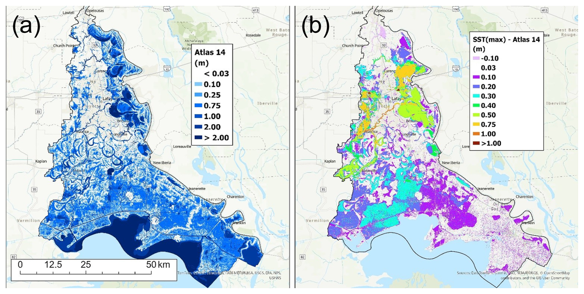
Figure 3 Spatial maps showing the basin-wide inundation depths produced by the NOAA Atlas 14 design storm (a) and the depth differences between the SST_max composite and Atlas 14 (SST_max-Atlas 14; b). (Sources: Esri, NASA, NGA, USGS, CONANP, TomTom, Garmin, SafeGraph, FAO, METI, NOAA, EPA, NPS, USFWS, © OpenStreetMap contributors, and the GIS User Community. Map created using ArcGIS^® software by Esri | Powered by Esri).

4.1 Distribution of Inundation Depths

Figure 4 presents the distribution of inundation depths for the Atlas 14 simulation and for each SST composite. Across all scenarios (Atlas 14 and the different SST composites), the depth distributions are strongly right-skewed, characterized by numerous shallow inundations and a progressively thinner upper tail. This form is consistent with the lognormal curves fitted to each scenario, whose corresponding parameters (μ_ln, σ_ln) are displayed in their respective panels. These parameters provide a summary of the distributional behavior and reveal two important patterns.

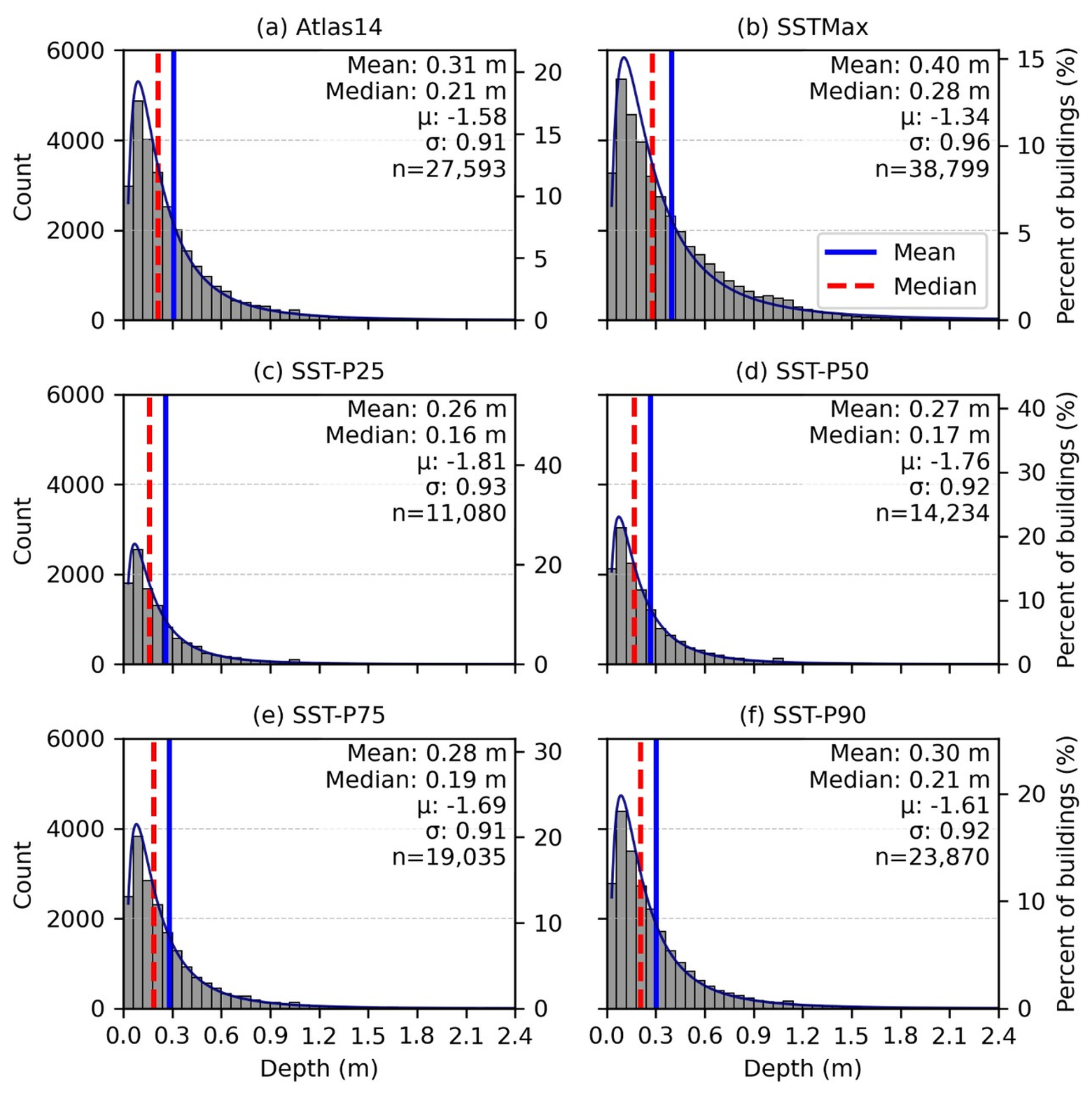
Figure 4 Histograms showing the distribution of inundation depths derived from the uniform rainfall-based inundation map (a) and from SST-based composite inundation maps (b through f). Each panel shows the median inundation depth (vertical red dashed line) and mean depth (vertical blue line). The fitted lognormal distribution parameters and the number of inundated buildings (n) are also reported in each panel. In all panels, “count” refers to the number of inundated structures within each inundation-depth bin. The SST composite scenarios include SST_max (b) and composites corresponding to the 25th, 50th, 75th, and 90th percentiles (c through f), respectively.

First, the shape parameter σ_ln, which represents the dispersion of the depths, is stable across all scenarios. In the Atlas 14 case and in each of the SST percentile composites, σ_ln varies only modestly, indicating that the fitted depth distributions maintain a similar right-skewed spread between shallow and deep inundation depths. The stability of σ_ln suggests that while a storm's spatial variability can change how many buildings flood or how deep the inundation can get at these locations, it does not fundamentally alter the relative dispersion of flooded-building depths across the fitted distributions.

Second, the location parameter μ_ln, which controls the central tendency of the lognormal distribution, shifts noticeably across the scenarios. Atlas 14 produces a distribution centered around μ_ln values consistent with a median depth near 0.2 m, reflecting broad but relatively uniform inundation (i.e., no disproportionate concentration of impact areas). The SST percentile composites P75 through P90 produce values that closely track those of Atlas 14, indicating that many SST realizations generate storms whose basin-wide impacts, in terms of flood severity, resemble those of Atlas 14.

In contrast, the SST_max composite displays a substantially higher μ_ln value, corresponding to a median depth near 0.3 m and a visibly heavier upper tail. This upward shift in μ_ln should not be interpreted as a response to basin-average rainfall volume alone. Although the baseline Atlas 14 storm has a larger basin-scale rainfall depth than the mean SST realization, the SST_max composite reflects localized storm placements that can produce deeper inundation over developed or hydraulically sensitive portions of the basin. This is because the average basin rainfall accumulation across all SST realizations is 238.1 mm, while the uniform Atlas 14 depth after TP40 reduction is 310.0 mm. Thus, it is likely that spatially concentrated rainfall cores produce deeper inundation, increasing the central tendency of depths and expanding the upper tail beyond what the uniform deterministic storm produced.

These μ_ln and σ_ln patterns indicate that the fitted depth distributions retain a broadly similar right-skewed shape across scenarios, while the location and upper-tail behavior are more strongly influenced by the spatial distribution of rainfall. This behavior is consistent with the contrast between the single spatially uniform Atlas 14 rainfall field and the spatially variable storm placements represented by the SST composites, which can produce localized deeper inundation and expose additional buildings not inundated under the baseline Atlas 14 scenario.

4.2 Divergence in Aggregate Losses

Figure 5 summarizes flood impacts in terms of (a) inundation depth, (b) per-structure loss value, USD, and (c) basin-wide aggregate impact both in structure numbers and loss in value. These panels demonstrate two important aspects of the relationship between storm choice and economic losses.

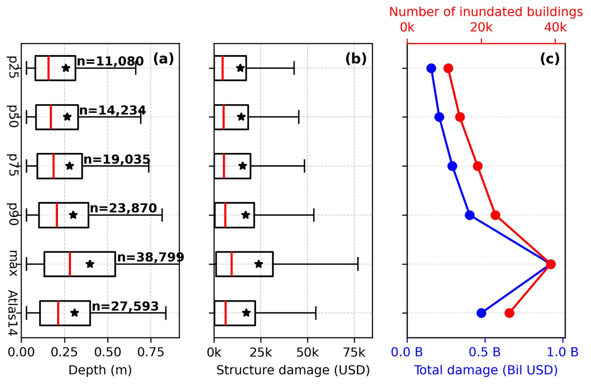
Figure 5 Box plots of flood depth (a) and structure damage (b) across all inundation scenarios. Black stars indicate the mean and the red line within each box indicates the median; n denotes the number of inundated buildings. Panel (c) shows total estimated damage (billions USD; blue line, bottom x axis) and the total number of inundated buildings (red line, top x axis).

First, the baseline Atlas 14 simulation results in a high-severity outcome comparable to upper-percentile SST composites (P75 and P90). The total structure damage produced by Atlas 14 is approximately USD 0.477 billion, slightly exceeding that of the SST 90th-percentile composite. This similarity is partly explained by rainfall volume: the TP40-adjusted Atlas 14 areal rainfall depth is 310 mm, whereas the mean basin-average 24 h accumulation across the 50 SST realizations is approximately 238.1 mm. However, the SST ensemble also shows that rainfall volume alone does not determine damage. Across the 50 SST realizations, basin-average rainfall-depth rank does not closely match total structure-damage rank (Fig. S1 in the Supplement), indicating that storm placement relative to developed flood-prone areas also affects losses.

Second, even though Atlas 14 aligns with the upper decile of the SST composites, it does not capture the highest plausible losses (middle and right panels). For example, the SST_max composite produces approximately USD 0.923 billion in total structure damage (Fig. 5c, blue line), substantially exceeding both the Atlas 14 estimate and the SST percentile composites. This divergence is consistent with localized rainfall intensities occurring over developed flood-prone areas, a condition that is represented in the SST ensemble but not in the spatially uniform Atlas 14 rainfall field. In this sense, the uniform Atlas 14 storm represents a widespread high-volume design event, as shown by its larger basin-average rainfall depth relative to the individual SST realizations (Fig. S2). However, the weak relationship between basin-average rainfall accumulation and total structure loss across the SST realizations indicates that spatial storm placement also contributes to the loss divergence. The increase in total loss is associated with both the larger number of impacted buildings and the higher average depth per impacted building (Fig. 5). The spatial difference map (Fig. 3, right panel) shows that positive flood-depth differences are concentrated in populated areas, particularly near Lafayette-Scott, contributing to the divergence in basin-wide damage. This observation emphasizes that a portion of the additional SST-driven damage arises from localized pluvial flooding in developed areas, where intense rainfall placement can increase building-level inundation outside the main river corridor. These losses are therefore not only a function of basin-wide flood severity, but also of how spatial rainfall organization interacts with locally flood-prone terrain.

In addition to the baseline Atlas 14 simulation, we performed three Atlas 14 sensitivity simulations to examine whether the deterministic design-storm comparison was strongly affected by selected Atlas 14 assumptions. These tests were motivated by the fact that the Atlas 14 and SST simulations differ not only in spatial rainfall structure, but also in how rainfall depth and temporal distribution are defined. The first sensitivity case used the upper bound of the NOAA Atlas 14 90 % confidence interval (389.3 mm after applying the TP40 reduction), with the same TP40 depth-area adjustment and 50 % alternating-block temporal pattern used in the baseline Atlas 14 simulation. The other two sensitivity cases retained the baseline Atlas 14 rainfall depth but shifted the alternating-block peak to 25 % and 75 % of the 24 h storm duration to evaluate sensitivity to temporal distribution. The upper 90 % confidence-bound Atlas 14 storm increased total structure damage to approximately USD 0.738 billion, while the 25 % and 75 % peak-timing variants produced approximately USD 0.426 billion and USD 0.495 billion, respectively. Although the upper 90 % confidence-bound Atlas 14 case is useful for testing rainfall-depth uncertainty, applying this upper-bound depth uniformly across the entire basin represents a conservative stress test rather than a physically typical storm realization, because it imposes high rainfall over all drainage areas simultaneously and can therefore overwhelm the drainage network more broadly than a spatially variable storm would. These results indicate that Atlas 14 rainfall-depth uncertainty has a larger effect on structure damage than the tested temporal peak-placement changes. However, all Atlas 14 sensitivity cases remain below the SST_max composite damage estimate of approximately USD 0.923 billion (Figs. S3–S4).

4.3 Quantifying the Exposure Gap

Next, we evaluated disagreement between the baseline Atlas 14 inundation map and the SST_max composite in both directions. This two-sided comparison is important because a deterministic design storm can also inundate structures that are not inundated in the SST_max composite. In this case, however, the Atlas 14-only group was small, containing 312 buildings and contributing approximately $2M in structure damage. Approximately 50 % of the Atlas 14-only buildings had inundation depths of 0.03 m or less, and 75 % had depths of 0.06 m or less, which explains their limited aggregate damage contribution (Figs. S5–S7). Because the reverse disagreement was small in both building count and damage, the remainder of this section focuses primarily on the larger SST-exclusive exposure gap: buildings inundated in at least one SST realization but not under Atlas 14. Figure 6 summarizes this SST-exclusive group, including the number of impacted structures, their inundation depths, and their corresponding structure losses.

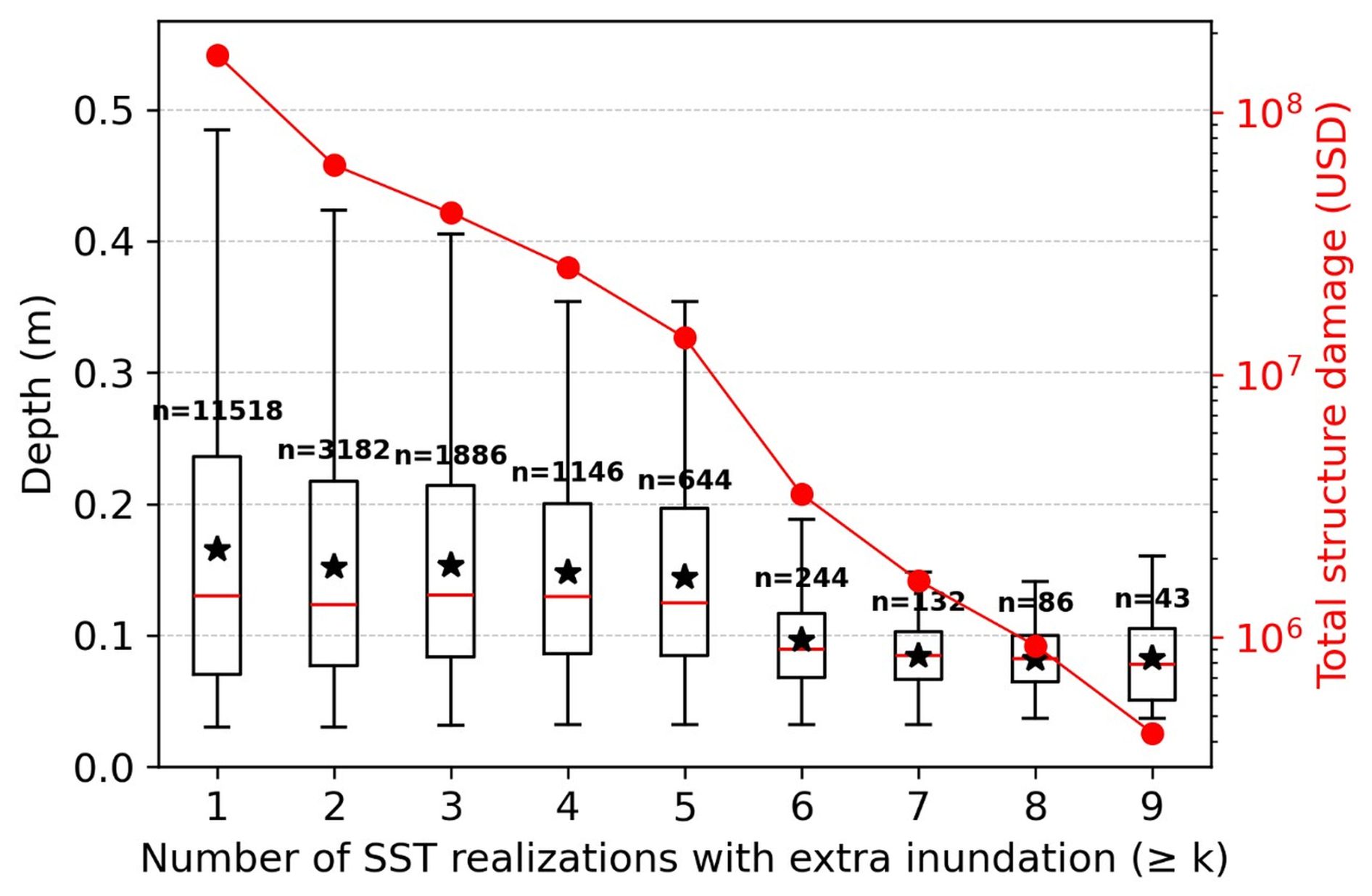
Figure 6 Depth metrics and aggregate damage estimates based on the number of times a set of structures was inundated by SST realizations but not by Atlas 14, occurring at least k times. Inundation depths are shown using box plots (left y axis, black), where the solid black star represents the mean depth and the red line within each box represents the median depth. The total number of inundated buildings included in each box is shown as (n). Total structure damage for each group is represented by solid red dots (right y axis, red).

This gap includes 11 518 impacted structures that were not impacted in the Atlas 14 scenario. A large portion of the SST-exclusive structures were inundated in one to four SST realizations (> 1000 structures), with the frequency decreasing sharply beyond that point. This indicates that much of the SST-exclusive exposure occurs only under specific storm-placement conditions within the 50 analyzed realizations.

Median inundation depths for the SST-exclusive structures are shallow, ranging from 0.08 to 0.13 m across the frequency groups. Although these median depths correspond to modest damage fractions for individual structures, the aggregate loss reaches approximately USD 110 million because the group contains many buildings and includes a subset of structures experiencing deeper inundation. Thus, the SST-exclusive exposure gap is important primarily as an aggregate building-level loss signal, not because the median inundation depth for each frequency group is large.

4.4 Spatial Intensification of Inundation Clusters

So far, we have characterized the differences between Atlas 14 and SST in terms of inundation depth, number of impacted structures, and the monetary value of structure losses. Here, we expand our investigation by identifying the spatial distribution and the specific locations where disproportionate differences in impacted structures occur. Figure 7 compares the spatial density of inundated buildings under the Atlas 14 and SST_max scenarios using the KDE-based clustering analysis described in Sect. 3.3.2. As noted in Sect. 3.3.2, we also tested the sensitivity of the KDE results to comparable bandwidth factors; these tests changed the local smoothness of the density surfaces but did not alter the dominant cluster locations or the interpretation of the Atlas 14–SST_max differences. The cluster patterns show that both approaches identify the main low-lying flood-susceptible regions (Fig. 1d), but two developed areas show stronger impacts under SST_max. The largest differences in cluster size and intensity occur in the relatively densely populated areas of Lafayette-Scott and Abbeville. In the case of Atlas 14, KDE clusters are visible at these locations; nevertheless, they are relatively moderate in both size and intensity. Under SST_max, the same locations exhibit more concentrated, higher-intensity clusters, indicating a greater number of impacted structures. This pattern suggests that these areas are more sensitive to localized rainfall placement than other populated portions of the VRB. This clustering pattern is broadly consistent with the spatial distribution of inundation-depth differences shown in Fig. 3; however, some locations with similar depth-difference patterns do not show the same increase in impacted-structure density. For example, populated areas around the main stem of the Vermilion River west and south of Lafayette show depth differences without the same degree of cluster intensification. This discrepancy motivated the HAND-based analysis in Sect. 4.5.

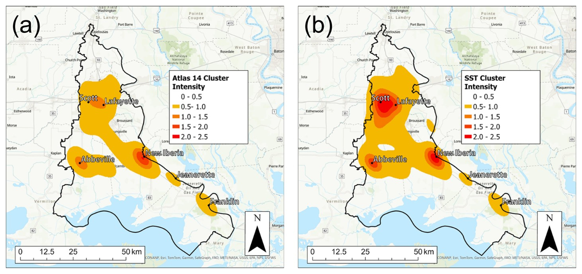
Figure 7 Spatial maps showing KDE-based clustering of inundated structures for the baseline Atlas 14 scenario (left) and SST_max composite (right). (Sources: Esri, NASA, NGA, USGS, CONANP, TomTom, Garmin, SafeGraph, FAO, METI, NOAA, EPA, NPS, USFWS, © OpenStreetMap contributors, and the GIS User Community. Map created using ArcGIS^® software by Esri | Powered by Esri).

4.5 Relationship Between Cluster Intensification and HAND

To investigate the underlying drivers of the intensified SST_max clusters, we visually inspected various topographic and drainage network characteristics at these locations. The topographic variables we investigated included elevation and slope, while the drainage network characteristics included the total number and size of the surrounding drainage channels and the proximity of the structures to the channels. We also compared building density in these areas with other densely populated portions of the VRB. This inspection showed a consistent spatial pattern: the largest differences in cluster intensity did not occur in the lowest floodplain areas, which tended to flood under both Atlas 14 and SST_max, nor in high-terrain areas that rarely flooded under either scenario. Instead, the discrepancies were concentrated in intermediate terrain-transition zones between low floodplain areas and upland terrain. Additionally, the size and depth of the channels draining those areas were relatively modest. These observations suggested that HAND could provide a useful terrain-based diagnostic for identifying where rainfall representation most strongly alters inundation patterns. To evaluate this hypothesis, we calculated the HAND (Fig. 8) surface as described in Sect. 3.3.2.

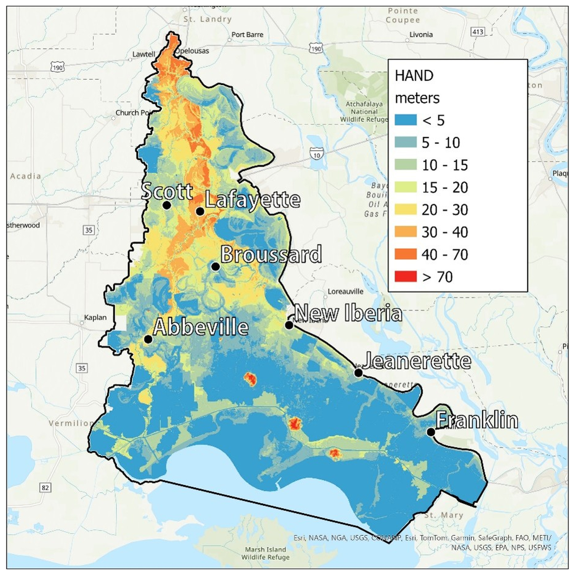
Figure 8 A spatial map depicting the calculated HAND distribution for the VRB. (Sources: Esri, NASA, NGA, USGS, CONANP, TomTom, Garmin, SafeGraph, FAO, METI, NOAA, EPA, NPS, USFWS, © OpenStreetMap contributors, and the GIS User Community. Map created using ArcGIS^® software by Esri | Powered by Esri).

Figure 8 shows that the lowest HAND values (light blue) delineate the primary floodplain flat areas, including inland-coastal zones in the south, swamp areas near the east-central portion of the VRB, and shallow wetlands across the basin. Mid-range HAND values between 10 and 30 m (green to yellow hues) occupy extensive areas in and around West Lafayette, Scott, Abbeville, and portions of New Iberia. Higher HAND values (orange hues) mainly cover the portion of the areas immediately surrounding the main stem of the Vermilion River, starting north of the city of Abbeville and extending further north past the city of Lafayette. Visual comparison between Fig. 8 and the spatial distribution of SST_max–Atlas 14 inundation-depth differences (Fig. 3, right panel) shows that the most substantial positive differences at populated areas occur within zones dominated by mid-range HAND values.

In Fig. 9, we further examine the association between HAND and the increase in the number of structures impacted by plotting the number of inundated structures for each HAND value. The gray bars represent buildings inundated under Atlas 14 within each 1 m HAND interval, while the red bars represent SST_max-only buildings. The blue curve is the cumulative distribution function (CDF) of the number of Atlas 14 inundated structures while the red curve is the CDF of the SST_max-only difference set.

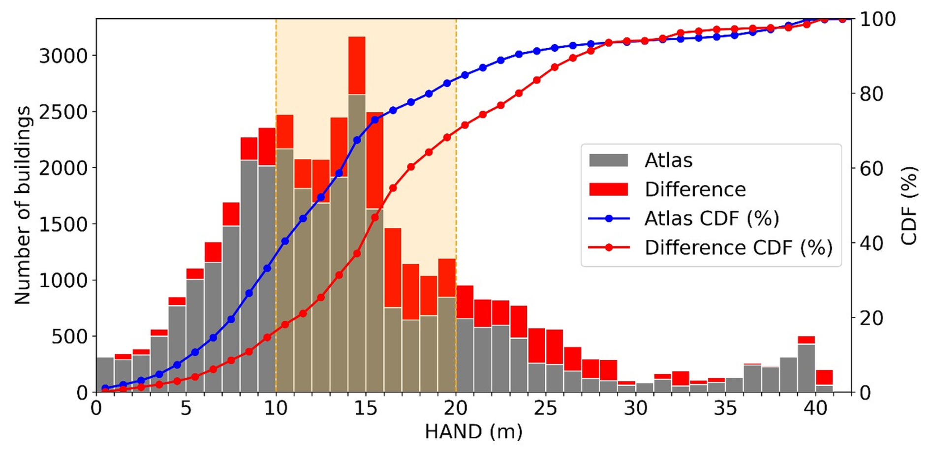
Figure 9 Bar chart showing the number of inundated buildings across HAND values. Gray bars represent the buildings that were inundated during the Atlas 14 scenario. The red bars represent buildings inundated under SST_max but not under Atlas 14. The blue and red lines show the corresponding cumulative distribution functions for Atlas 14 and SST_max-only buildings, respectively. The orange shaded area represents the HAND interval containing the middle 60 % of the SST_max-only difference set.

As expected, the Atlas 14 CDF rises rapidly at low HAND values and reaches approximately 75 % of its inundated structures near a HAND value of 15 m, after which it starts to level off. This is because uniform rainfall predominantly floods the relatively highly vulnerable portions of the landscape while having less impact on structures situated at higher HAND elevations. On the other hand, the difference CDF (red) begins to significantly increase near a HAND value of 10 m, then rises steadily through mid-range HAND values, and does not flatten until approximately a HAND value of 28 m. This demonstrates that the disagreement between the two CDFs is concentrated in the intermediate HAND range, where buildings lie near their potential inundation thresholds and are sensitive to local flooding caused by concentrated rainfall clusters.

To quantify this sensitivity, we computed the area between the two CDFs and identified the HAND interval responsible for the middle 60 % of SST-Atlas divergence (Fig. 9, orange shaded area). This interval lies between HAND values of 10 and 20 m. Notably, this HAND range aligns closely with the typical HAND values in the Lafayette-Scott and Abbeville neighborhoods highlighted in Fig. 8. This supports the interpretation that the KDE cluster intensification shown in Fig. 7 is associated with the HAND distribution differences shown in Fig. 9.

5 Discussion

In this study, we examined how the storm representation influences the modeled flood depth and extent, as well as the resulting losses to exposed structures. Although deterministic, spatially uniform Atlas 14-based storms are widely accepted as the current state of practice in flood risk mapping, the effects of applying this simplified rainfall representation on flood risk and structural losses are underexamined. By comparing the inundation from the Atlas 14-based storm with inundation from 50 SST-based storm realizations, we identified areas where the deterministic design storm produced lower exposure and damage estimates than the SST ensemble. We also used KDE and HAND analyses to examine where the Atlas 14 and SST_max differences were spatially concentrated and how those differences related to terrain position.

The results of the comparison showed clear differences in inundation depth, extent, and basin-wide economic loss estimates. Across all rainfall scenarios (i.e., Atlas 14 vs. SST percentile-based composites), the depth distributions for the inundated buildings were strongly right-skewed and well approximated by lognormal fits, with similar shape parameters across scenarios. In the fitted building-level depth distributions, Atlas 14 was comparable to the SST 90th-percentile composite, while SST_max had higher central depths and a heavier upper tail. Basin-wide losses were consistent with this pattern: the Atlas 14 scenario resulted in approximately USD 0.477 billion in structure damage, while the SST_max composite reached approximately USD 0.923 billion. The two-sided exposure comparison showed that the dominant disagreement was the SST-exclusive group, with 11 518 structures inundated in at least one SST realization but not under the baseline Atlas 14 scenario. This group accounted for approximately USD 110 million in cumulative structure damage, despite shallow median depths across the exposure-frequency groups. Spatial clustering and HAND analyses showed that the largest SST_max–Atlas 14 differences were concentrated in developed intermediate-terrain areas, particularly near Lafayette-Scott and Abbeville.

The similarity between Atlas 14 and the SST 90th-percentile composite reflects the smoothing effect introduced by how percentile composites are generated. In this sense, the per-pixel SST 90th-percentile calculation behaves like a low-pass filter on the ensemble, retaining recurring inundation patterns while reducing the influence of localized extremes that occur in only a small fraction of realizations. The Atlas 14 sensitivity simulations further support this interpretation. Using the upper bound of the NOAA Atlas 14 90 % confidence interval increased structure damage relative to the baseline Atlas 14 case, whereas shifting the alternating-block peak to 25 % or 75 % of the 24 h duration produced smaller changes. However, all Atlas 14 sensitivity cases remained below the SST_max composite damage estimate, indicating that conventional design-storm uncertainty affects the deterministic damage estimate but does not eliminate the upper-envelope differences produced by the SST ensemble.

The practical implication is that spatially uniform design storms can provide useful basin-wide design information, but they may not identify localized pluvial exposure in developed areas where storm placement interacts with local drainage and terrain-transition zones. This interpretation is consistent with pluvial-flooding studies showing that spatially and temporally variable rainfall can strongly affect urban inundation patterns and that stochastic rainfall-based approaches can help identify pluvial flood hotspots that may not be captured by deterministic design-storm assumptions (Simões et al., 2015; Mediero et al., 2022). The basin-wide HAND analysis helps identify where this limitation is most relevant: in this case, the largest SST_max-only building differences were concentrated in intermediate HAND zones, rather than only in the lowest floodplain areas. Merz et al. (2008) stated that in flood risk assessment, uncertainty in depth-damage calculations is more impactful during low-intensity events, while uncertainties in flood frequency analysis dominate during rarer events. These findings are consistent with recent SST-based flood-hazard and risk studies. Perez et al. (2024) extended the FFA-SST framework from peak-flow estimation to flood extent and population exposure, while Baer et al. (2026) compared design-storm and SST-based estimates of flood hazard and expected annual damage. The present study complements these efforts by focusing on a detailed engineering-design case: how a 100-year, 24 h deterministic design storm and 50 SST-derived rainfall realizations propagate through a coupled HEC-HMS/HEC-RAS and building-level consequence workflow. This aligns with Wing et al. (2022), who showed that deterministic flood hazard maps do not cover a substantial fraction of flood-prone areas. In the context of the present study, this suggests that FEMA floodplain maps and design-storm-based hazard products remain important regulatory and planning tools, but they may not fully capture rainfall-driven pluvial exposure outside the main river corridor. Our findings are also consistent with Gutenson et al. (2023) and Grimley et al. (2025), who showed that estimates of flood exposure and damage can change significantly depending on how the contributing flood drivers are represented. In the present case, this means that mitigation planning, benefit-cost screening, and local drainage prioritization may benefit from supplementing deterministic design-storm simulations with SST-based or other spatially variable rainfall analyses, especially where localized rainfall placement controls building-level consequences. Wright et al. (2026) emphasized the value of ensemble-based rainfall representations for accounting for spatial and temporal uncertainty in hydrologic prediction. Our results extend this point to building-level consequences by showing that, in this case study, the SST realizations identified localized exposure and upper-tail damage concentrations that were not reproduced by the baseline spatially uniform design storm. The implication is not that Atlas 14 should be replaced in design practice, but that spatially uniform design-storm simulations should be supplemented where localized pluvial flooding and building-level consequences are important.

A few limitations of the analysis should be noted. This study compares two rainfall-forcing interpretations of a 1 % annual exceedance probability, 24 h event in one basin: a baseline Atlas 14-based spatially uniform design storm and 50 SST-derived rainfall realizations. Both rainfall-forcing approaches represent inland rainfall-driven flooding, and neither is intended to represent all flood-generating processes relevant to coastal Louisiana. There are, however, other representations that include, for example, different types of coincident flood drivers such as storm surge-rainfall combinations associated with tropical systems, or the compounding effects of spatial or temporal storm clustering (Amorim et al., 2025; Liu et al., 2025; Grimley et al., 2025). The focus here is narrower: to evaluate how a spatially uniform deterministic design storm and spatially variable SST rainfall realizations propagate through the same hydraulic and consequence-modeling workflow to affect building-level exposure and structure damage estimates. A second limitation is that the SST results depend on the selected transposition domain and parent-storm catalog. The domain used here was selected to represent broadly similar extreme-rainfall conditions around the VRB, but alternative domain choices could change the storms available for transposition and therefore the resulting SST rainfall fields. Recent work by FitzGerald et al. (2026) introduced an objective SLAM procedure for identifying homogeneous storm-transposition regions, highlighting the importance of reproducible SST-domain delineation for broader applications. We did not conduct a formal sensitivity analysis using alternative SST domain definitions. Another limitation of this work is the computational cost of the modeling approach. The coupled HEC-HMS/HEC-RAS model used in this study provides a detailed representation of channels, hydraulic structures, and storage areas, which is needed to simulate complex flood regimes within the watershed. This level of detail comes at a computational cost and restricts the number of simulations that can be executed in a reasonable timeframe. Merz et al. (2008) also discussed the problem of computational costs in the hydrologic sciences and how they limit practitioners' ability to conduct ensemble-based analyses. The 50 SST realizations used here therefore represent a computationally feasible sample of plausible 100-year, 24 h SST rainfall scenarios, not an exhaustive sample of all possible SST storm placements or rainfall-frequency outcomes. Unlike full FFA-SST or probabilistic risk workflows, this study does not estimate complete flood-frequency or damage-frequency curves, expected annual damage, or uncertainty bounds across many return periods. Such broader workflows require many more hydrologic, hydraulic, and consequence simulations than were feasible with the detailed HEC-HMS/HEC-RAS and building-level damage workflow used here. In contrast, simpler models such as SFINCS (Grimley et al., 2025) can support hundreds or thousands of simulations in a reasonable amount of time, but they may simplify hydraulic controls, storage areas, and channel bathymetry that are important for the VRB application.

6 Conclusions

This study compared building-level flood exposure and structure damage estimates produced by selected 100-year, 24 h rainfall representations in the Vermilion River Basin (VRB), south Louisiana. The primary comparison was between a baseline spatially uniform NOAA Atlas 14 design storm, adjusted using TP40 depth-area relationships, and 50 stochastic storm transposition (SST)-derived rainfall realizations generated from gauge-adjusted radar rainfall fields. Additional Atlas 14 sensitivity simulations were used to evaluate how rainfall-depth uncertainty and temporal peak-placement assumptions affected the baseline deterministic design-storm result. All scenarios were evaluated under a common hydrodynamic and damage-assessment framework. The study's main findings are summarized as follows:

1. Flood exposure and structure damage differed substantially between the baseline Atlas 14 scenario and the SST ensemble. In the VRB, SST_max inundated 11 518 structures that were not inundated by the baseline Atlas 14 storm, corresponding to approximately USD 110 million in additional structure damage. The baseline Atlas 14 simulation produced approximately USD 0.477 billion in structure damage, while the SST_max composite produced approximately USD 0.923 billion. Although the TP40-adjusted Atlas 14 rainfall depth was larger than the mean SST basin accumulation (310 mm vs. 238.1 mm), localized SST storm placements produced larger upper-envelope exposure and damage than the baseline spatially uniform design storm.

2. The largest Atlas 14–SST_max differences were spatially concentrated rather than uniformly distributed across the basin. KDE clustering showed stronger SST_max impact clusters near Lafayette-Scott and Abbeville, while the HAND analysis showed that many SST_max-only buildings were concentrated in intermediate HAND zones rather than only in the lowest floodplain areas. This indicates that the additional SST exposure was concentrated in developed terrain-transition areas where localized pluvial flooding can alter building-level inundation outcomes.

3. Practitioners should use spatially variable rainfall scenarios as a complement to deterministic design-storm simulations when evaluating building-level flood consequences. Atlas 14-based design storms provide a standardized and reproducible rainfall input for conventional design applications, but a single spatially uniform storm cannot represent the range of storm placements that may produce localized pluvial flooding in developed areas. Pairing deterministic design-storm simulations with SST-based or other spatially variable rainfall scenarios can help identify exposure hotspots, upper-envelope damage concentrations, and locations where mitigation or drainage improvements may be most sensitive to rainfall placement.