Areal reduction factors from high-resolution rain gauges in Austria

Areal Reduction Factors (ARFs) are widely used to convert point design precipitation derived from intensity–duration–frequency (IDF) curves into areal precipitation values for hydrological design. Despite their importance, ARFs remain highly uncertain, particularly for short durations and small areas, due to insufficient representation of precipitation spatial variability. In this study, ARFs are empirically derived using a fixed-area approach for the Feldbach region in southeastern Austria using the WegenerNet, a dense rain gauge network with high temporal resolution (5 min) for the period 2007–2022. The results confirm that ARFs generally increase with duration and decrease with area, while pronounced dependencies on season and return period are observed, particularly for sub-hourly durations. Contrary to common assumptions, an application of ARF is required even for areas as small as 1 km², indicating that point measurements and pixel-based precipitation estimates cannot be considered equivalent. For sub-hourly durations, ARFs increase partially with the return period. Seasonal analysis reveals smaller ARFs during spring and summer, associated with convective precipitation, and higher values during winter. The relationship between ARFs and topography is found to be weak, with only negligible correlations between ARFs and station elevation.

1 Introduction

Design precipitation plays a crucial role in a wide range of applications in planning, design, and maintenance of water infrastructure. Design precipitation is commonly derived from Intensity-Duration-Frequency (IDF) curves, which describe the relationship between precipitation intensity, duration, and return period. Conventionally, this tool is provided based on Extreme Value Analysis (EVA) of point precipitation measurements at rain gauges, which are not representative for larger areas, such as catchments. Associating the point design precipitation values with an area leads to an overestimation of the areal precipitation, as precipitation is a highly variable spatial phenomenon. Areal Reduction Factors (ARFs) are used in combination with IDF curves to convert point precipitation design values P_p to areal design precipitation values P_a by multiplying the point value by ARF, which represents the ratio of the average areal precipitation to point precipitation in the area of interest:

$$\begin{array}{}\text{(1)}& P_{\mathrm{a}}=\mathrm{ARF}\cdot P_{\mathrm{p}}\end{array}$$

ARFs can be distinguished in (a) analytical and (b) empirical approaches. In the analytical approach, the ratio is calculated based on the mathematical determination of the physical rules that govern the precipitation behavior, relying on simplifying assumptions. The empirical approach, on the other hand, relies solely on the available data and calculates the ARF based on the observations. Although computationally more demanding, the latter approach is more representative if the data is acceptably accurate (Svensson and Jones, 2010) and the time series has a sufficient length. Besides the analytical vs. empirical subcategories, ARF calculation methods can also be categorized as fixed-area or storm-centered methods. The fixed-area methods focus on a geographically fixed area of interest and calculate the ARF using the observed point and observed or regionalized areal precipitation time series, considering the study area. The storm-centered methods, on the other hand, focus on the storm cell as the area of interest and calculate the ARF as the ratio of the areal precipitation of the storm-cell to the precipitation depth of the cell center, namely the cell with the highest precipitation depth (Biondi et al., 2021).

One of the first studies to formulate the ARF is from the U.S. Weather Bureau (1957a, b), where they calculated the ARF as the ratio of the averages of annual maximum areal and point precipitation. Using a fixed-area approach, the average values are calculated across all years and stations without consideration of the return period. Thereafter, Bell (1976) proposed an empirical method where the return period is taken into account by determining the theoretical probability distribution of the annual maximum areal and point precipitation. Since then, many studies like Kao et al. (2020) have confirmed the necessity of including the frequency in the calculation. Parallel to the commonly used empirical fixed-area methods, analytical storm-centered approaches were developed by studies like Rodriguez‐Iturbe and Mejía (1974) where they conclude that the ARF depends only on the expected correlation coefficient between the precipitation value at two random points within the area of interest. Sivapalan and Blöschl (1998) extended the method of Rodriguez‐Iturbe and Mejía (1974) by considering the area, spatial correlation, duration and return period. Asquith and Famiglietti (2000) and De Michele et al. (2001) are examples of empirical storm-centered and analytical fixed area approaches respectively, where the former offers an annual maximum series approach and shows the importance of including the return period in the calculation of ARF. The latter calculates the ARF using the scale-invariance of the precipitation, deriving the factors from the spatial scaling properties of precipitation in time and space.

Many studies have focused on factors affecting the ARF and how it changes in relation to these factors. Numerous studies have identified duration, area, return period, event type, location, topography, calculation method, and rain gauge density as significant influences. The general knowledge in the field suggests that ARF increases with increasing duration (NERC, 1975; Kim et al., 2019; Kao et al., 2020), decreases with increasing return period (Asquith and Famiglietti, 2000; Allen and DeGaetano, 2005; Breinl et al., 2020; Kao et al., 2020), decreases with increasing area (NERC, 1975; Sivapalan and Blöschl, 1998; Ramos et al., 2005; Breinl et al., 2020; Kao et al., 2020; Kim et al., 2019) and decreases with increasing spatial variability of events which is directly associated with increasing convective behavior and attributed to the warm seasons (Kim et al., 2019; Kao et al., 2020; Allen and DeGaetano, 2005). More detailed investigations reveal that, for example, the decrease of ARF with increasing return period is more pronounced for shorter duration, and attribute this to the higher convective activity in temporally shorter events (Breinl et al., 2020). Conversely, an increase of ARF with increasing return period is shown for the two durations of 12 and 24 h by Chang et al. (2023) where they investigate events spanning from 1 to 48 h. Furthermore, the decrease of ARF with increasing area is steeper for shorter duration (NERC, 1975; Sivapalan and Blöschl, 1998) specifically for durations shorter than 90 min (Ramos et al., 2005). Allen and DeGaetano (2005) show that ARF decreases more sharply with area in warm months of April to September. Goshtasbpour and Haberlandt (2025) came across a significant number of cases where the areal precipitation and thus the ARF increases with increasing area for durations higher than 12 h. They assume that the current fixed-area approach, combined with the low availability of dense station networks fails to capture the spatial variability of the extreme precipitation. Kim et al. (2019) quantifies the spatial variability by calculating the coefficient of variation of the pixel values within a storm cell and prove it to be a strong predictor for the ARF with an inverse relationship. Regarding location, there are contradictory results. Studies like Omolayo (1993) prove that ARFs from the US apply to Australia and Allen and DeGaetano (2005) claim the same for the two states of New Jersey and North Carolina within US. On the other hand, Kao et al. (2020) prove in their country-wide study that there is a high geographical variability of ARF across the US and the values of one location should not be arbitrarily applied to other locations. Pavlovic et al. (2016) focused their work on the intercomparison of a selection of fixed-area methods, two analytical and two empirical methods and report that the method selection has a significant influence on the resulting ARF values.

In an extensive study, Chang et al. (2023) compare the ARFs estimated by four empirical methods. They investigated the effect of local topography and quantified the effect of rain gauge density on ARFs in the coastal city Shenzhen, China. Utilizing a 10-years long station data sets from a sparse network with 36 stations and another more dense network with 102 gauges with 5-years long records with an hourly resolution Chang et al. (2023) conclude that the ARFs in the mountainous part of their study area were lower than those in the regions with relatively flat terrain, due to the more substantial spatial variability of precipitation possibly caused by the topographical effect. Supporting Kao et al. (2020) findings, Chang et al. (2023) suggest that regions with different landscapes are characterized by different ARFs even within a small catchment (less than 2000 km²) and using a constant ARF across broad areas might be inappropriate. Further, they report a tendency to overestimate ARF for the less dense rain gauge network, especially for short durations. Short-duration events of convective nature usually have a relatively small spatial extent. Often these events are not recorded with sparse rain gauges, which explains the sensitivity of ARFs to the density of rain gauges.

Since the fixed-area estimation of ARFs in regions with spare observation networks is highly uncertain, Lutz et al. (2024) analyze regional and seasonal ARFs for Norway based on three different gridded data sets, two station-based and one reanalysis product. They conclude that the reanalysis product with hourly temporal and 3 km spatial resolution results in adequate and robust estimates of ARF. As dense station networks and station-based data sets with high spatial and temporal resolution and large covered areas are limited and not easily accessible, numerous studies use radar-based precipitation estimates, which are available for a few decades in some regions. Kao et al. (2020) compare five data sources: one gauge data set, three gauge-based gridded data sets and a radar-based data set in the United States (US). According to them, gauge data is the most reliable source for calculating ARF. Radar-based ARFs perform the poorest for high return periods due to the short length of the available time series, despite offering the best spatiotemporal resolution. The gridded data sets are proven not to be suitable for sub-daily ARFs due to their low temporal resolution. Other radar-based studies (Thorndahl et al., 2019; Kim et al., 2019; Wright et al., 2014) use the continuous temporal fields of precipitation estimates and developed different storm-centered methods. While Thorndahl et al. (2019) offers a novel approach for storm-centered calculation of ARF, Kim et al. (2019) focus on the influence of spatial variability of precipitation on ARF. Not so far off, Wright et al. (2014) report a high variability in storm-centered ARF estimates of North Carolina, United States, where the variability relies highly on the storm type, which implies that not distinguishing between event types in ARF estimation, can lead to systematic errors and overestimation of design values.

To our knowledge, only a few studies exist on sub-hourly ARFs, and none uses a dense rain gauge network like the WegenerNet (Fuchsberger et al., 2021), which is used in this study. We utilize these high resolution data to calculate the ARF using an empirical fixed-area method and investigate the relationship between sub-hourly ARF and duration, return period, area and season.

The novelty of the current study is estimating ARFs for sub-hourly durations from a rain gauge network with such a high spatial density. The high network density minimizes the risk of missing storms and storm centres, which are essential for a robust ARF estimation. While our findings confirm the influence of duration, return period, area and seasons in general, new insights on the type of influence for e. g., return period, are gained.

The paper is structured as follows: Sect. 2 presents the study area and the data used in the study; Sect. 3 explains the methods for estimating ARFs, extreme value analysis, and calculating areal precipitation. The results are presented in Sect. 4 and discussed in Sect. 5. The conclusions are listed in Sect. 6.

2 Study Area and Data

2.1 Study Area

The study area is the Feldbach region located in the southeast of the federal state of Styria, Austria (Fig. 1). The eastern Styrian area is characterized by diverse meteorological and climatological conditions, as well as a varied orographic structure. The Feldbach is geographically part of the southeastern Alpine foothills. The landscape is composed partly of the East Styrian hills and the valley floors of the foothill region. The hills are characterized by elongated, often asymmetrical ridges with steep western slopes and more gentle eastern slopes. The elevation range in the study area spans from 250 to 598 m a.s.l. The valley floor of the foothill region consists of the broad alluvial valley of the Raab river, which stretches approximately 23 km within the study area and has a relatively uniform elevation ranging from 250 to 300 m a.s.l., resulting in a rather low gradient. The alluvial valley in the study area varies in width from 800 to 2500 m. The ridges are predominantly forested, while the slopes are mainly used for orchards and other agricultural activities. The valley landscape is also primarily used for agriculture, except for the town of Feldbach (Kabas et al., 2011). The climate of the study area is shaped, on the one hand, by the region's location in the southeastern Alpine foothills and its proximity to the Alpine arc itself and on the other hand, by factors affecting the overall Alpine climate. On a large scale, the Alpine climate is primarily influenced by the weather systems of the North Atlantic, the effects of the Mediterranean Sea, and the Eurasian landmass (Kabas et al., 2011). Based on the Köppen-Geiger climate classification, the Feldbach region can be categorized as cold climate without dry season but warm summers (Peel et al., 2007).

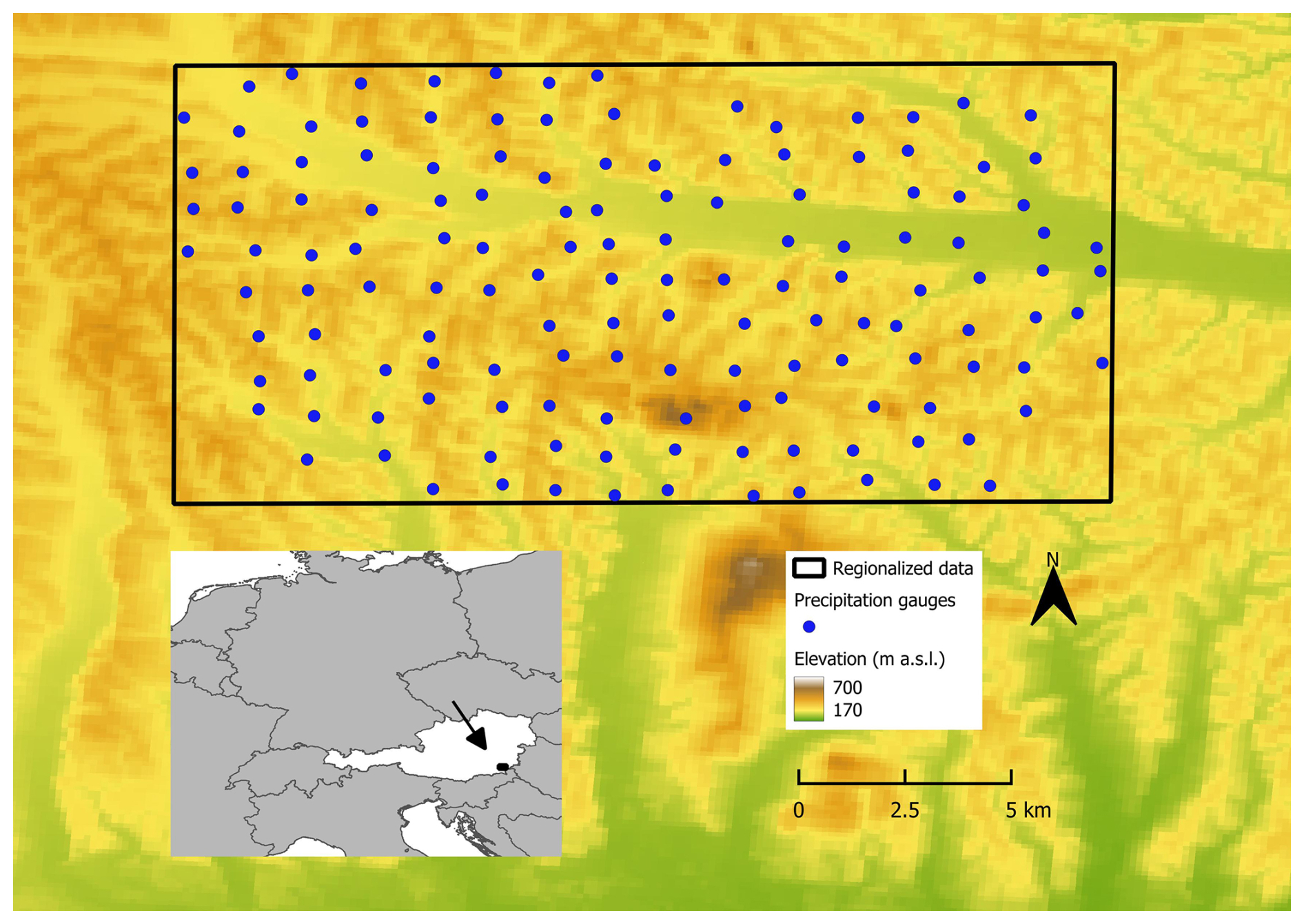
Figure 1 Precipitation gauges and raster extent of the regionalized precipitation data of the WegenerNet. The map in the lower left corner shows the location of Austria in central Europe (highlighted in white), and the WegenerNet within Austria (sources: European countries: Sevdari and Marmullaku, 2023; digital elevation model: Jarvis et al., 2008).

On a fine scale, the Feldbach region is dominated in summer by heavy rainfall from thunderstorms (Breinl et al., 2020). This is endorsed by lightning information accessible from the Austrian Lightning Detection and Information System (ALDIS; Schulz, 2005), indicating the federal states Styria (including the Feldbach region) and Carinthia as regions with highest frequency of thunderstorms (see Breinl et al., 2020). Furthermore, large hail events and severe wind gusts are typical for the Feldbach region according to the European Severe Weather Database (ESWD; Dotzek, 2009). The mean wet spell duration in summer is approx. 3 h, the overall mean dry spell duration ranges between 30 and 32 h (Breinl et al., 2021). Matulla et al. (2003) points out historical region-dependent differences in precipitation-generating processes on a monthly basis for Austria, but concludes that precipitation events in winter result from large-scale advective processes. Seibert (2007) identified the strongest precipitation events on a daily basis in the period July–October. Although Matulla et al. (2003) and Seibert (2007) use data sets with different temporal resolution and station density, their findings were combined by Breinl et al. (2021) with their own findings, classifying the Feldbach region as Eastern mixed region and thus highlighting its transition characteristic.

2.2 Data

The WegenerNet climate station network is characterized by its exceptionally high spatial density of climate stations. It is designed for long-term studies of small-scale weather and climate developments, providing measurements at high spatial and temporal resolutions. The network consists of 168 climate stations located in Austria, 155 of which have operated in the Feldbach region since 2007. Due to relocation of 12 stations during the study period these stations had to be removed from the data set and the remaining 143 stations are used for the analyses of this study. The studied time series spans from 2007 to 2022, 15 years with a temporal resolution of 5 min. Additionally, a regionalized raster product from the WegenerNet is used, which covers a total area of 330 km² with 75 × 110 grid cells. A grid of 200 m × 200 m in the Universal Transverse Mercator projection is available for each time step. The data collected by the climate stations undergoes an automated Quality Control System, followed by a Data Product Generator.

The Data Product Generator regionalizes the gauge-based time series with an inverse distance-squared method (IDSW; Fuchsberger et al., 2021). Inverse distance-based methods lead to similar results as Ordinary Kriging for a high station network density (Berndt, 2018). Also, additional improvements from e.g., external drifts, can be questioned for such a dense network. IDSW is able to represent the spatial variance of the precipitation field, by simultaneously representing the extreme values well due to favouring the immediate stations by squaring the distance. Using the regionalized data product also enables comparisons with other studies.

For a more detailed description of the study area and the WegenerNet data, the authors refer to Kabas et al. (2011) and Fuchsberger et al. (2021). For the validation of the estimated point precipitation extreme values the official Austrian design precipitation values from eHYD (Electronical HYdrographic Data) are applied.

3 Methodology

3.1 Areal reduction factor

The ARF is determined as the ratio of areal precipitation P_a(D,T) to point precipitation P_p(D,T) for each duration D and return period T of interest, as displayed in Eq. (2) (Verworn and Schmidtke, 2006):

$$\begin{array}{}\text{(2)}& \mathrm{ARF}(D,T)={\displaystyle \frac{P_{\mathrm{a}}(D,T)}{P_{\mathrm{p}}(D,T)}}\end{array}$$

where the P_a(D,T) and P_p(D,T) correspond to areal and point precipitation for given duration and return periods extracted from the time series using the method of Extreme Value Analysis (EVA) (DWA, 2012). The EVA method is elaborately described in the following subsection, followed by the description of how areal precipitation extreme values were derived.

3.2 Extreme Value Analysis

3.2.1 Point precipitation

For each station, the time series with an original temporal resolution of 5 min is calculated for different durations using a temporal moving window. The moving window is an interval with the length of $l_D=D/\mathrm{5}$ time steps for each duration D [min]. The window is shifted from the first step of the time series by a time increment of 5 min over the whole time series. The aggregated precipitation depth within the moving window is calculated to determine the extreme events of the whole time span. This has been done for 16 durations from 5 min to 24 h (D = 5, 10, 15, 20, 30, 45 60, 90, 120, 180, 240, 360, 540, 720, 1080 and 1440 min).

Due to the short length of the study period (n_yr = 15 years) the Peak-Over-Threshold (POT) is chosen over the Annual Maximum Series (AMS) to increase the sample size (as recommended by the DWA, 2012). For the calculation of the POT a threshold is chosen so that the extreme value sample will be approx. $l_{\mathrm{POT}}=n_{\mathrm{yr}}\cdot e=\mathrm{15}\cdot \mathrm{2.72}\simeq \mathrm{40}$ with Euler's number e. For this purpose, the aggregated precipitation depth series for each duration are sorted in descending order, and the 40 largest precipitation values are selected (DWA, 2012).

The independence of the extracted events is ensured by considering a minimum inter-event time (MIT) of MIT = 4 h for D ≤ 4 h, and MIT = D for D > 4 h. For each station and duration the POT is generated. Subsequently, an exponential distribution F(x) (see Eq. 3) with x as variable of interest (here: precipitation rate) and k as scale are fitted to the sample:

$$\begin{array}{}\text{(3)}& F\left(x\right)=\mathrm{1}-e^{-x/k},x\ge \mathrm{0}\end{array}$$

The exponential distribution function and the Weibull distribution function as its parent distribution are applied internationally for sub-daily precipitation extreme value analysis (e.g., Alexopoulos et al., 2023; Ebers et al., 2024; and within the TENAX model by Marra et al., 2024, with all subsequent applications). Furthermore, the Weibull-distribution function with powered-exponential tails is justified by thermodynamic arguments (Wilson and Toumi, 2005), and supported by recent recent studies (see Marra et al., 2024 for more details).

For design values, extreme precipitation values of certain return periods T are of interest, which can be expressed in general as:

$$\begin{array}{}\text{(4)}& P(X\le x)=F\left(x\right)=\mathrm{1}-{\displaystyle \frac{\mathrm{1}}{T}}\end{array}$$

For that, the empirical return period is calculated first for each POT event in the POT (Cunnane, 1978; DWA, 2012):

$$\begin{array}{}\text{(5)}& T_k={\displaystyle \frac{L+\mathrm{1}-\mathrm{2}\cdot \mathit{\alpha }}{k-\mathit{\alpha }}}\cdot {\displaystyle \frac{M}{L}}={\displaystyle \frac{L+\mathrm{0.2}}{k-\mathrm{0.4}}}\cdot {\displaystyle \frac{M}{L}}\end{array}$$

where M is the length of the time series in (years), L is the sample size and k is the rank of the event in the descending sorted POT. Cunnane (1978) has shown that each distribution function requires its own plotting position to avoid biased quantile estimation and suggested a value of α=0.44. Fuchs (1983) analysed different values for α, and identified 0.44 as most suitable alpha value by for the plotting position formula of the exponential distribution, leading to the values 0.2 (denominator) and 0.4 (numerator).

Instead of using the exponential distribution function in its arithmetic version, a geometric approach is chosen using probability plots. With the precipitation on the y-axis and the return period T on the x-axis the exponential distribution function will be a straight line in a semi-logarithmic plot, characterized by u as zero point shift and w as slope. Both, u and w, can be estimated as graphical parameters of the exponential distribution via regression functions and are linked as (Lengfeld et al., 2021):

$$\begin{array}{}\text{(6)}& T=e^{\frac{x-u}{w}}\end{array}$$

To avoid overlaps among the distribution functions for each D, a two-step double-logarithmic smoothing is applied over the parameters u and w (see DWA, 2012 for details). The described EVA was applied to the point time series for the entire year as well as for four seasons. Each year was divided into spring: March–May, summer: June–August, Autumn: September–November and winter: December–February.

3.2.2 Areal Precipitation

The areal precipitation needed for the calculation of the ARF is extracted from the raster-based data set of the WegenerNet. Initially, the grid cells corresponding to the study stations are located. Starting from the respective grid cell encompassing each station, square-shaped areas are constructed. It is assumed that a square is similar to the shape of the hydrological catchment around the station (Breinl et al., 2020). Other studies (Kang et al., 2019) suggest circular areas, but since square-shaped areas are computationally less demanding and only approximately 9 % of the area of a square does not lie within a circle of equal area, we chose squares.

Based on the grid resolution and its extent, 12 area sizes ranging from 1 km² (5 × 5 grid cells) to a maximum of 225 km² (75 × 75 grid cells) are chosen (A=1, 3.24, 9, 14.44, 25, 38.44, 49, 81, 121, 169, 201.64 and 225 km²). As the area size increases, there is a possibility that a part of the area window does not overlap with the study area. In that case, for that area size and that station, there will be no time series to consider. This implies that with increasing area size, the number of time series decreases. Due to the drastic decrease in the number of valid time series for area sizes above 81 km², the ARF analysis is limited to area sizes of up to 81 km².

For each station and area, the areal precipitation depth is calculated as the arithmetic mean of the pixel values within the covered area for each time step. The EVA, as described in the previous subsection, is applied to the generated areal time series. Each areal precipitation time series of each station is processed in the same way as the point time series for the EVA.

4 Results

In this section, the point and areal precipitation extreme values will be initially presented. Subsequently, the resulting ARFs will be described and analyzed with respect to area size, duration, return period and seasons. Finally, the regional patterns of ARFs and their relationship to topography are investigated.

4.1 Precipitation extreme values

The estimated precipitation point extreme values are depicted in Fig. 2. As expected, for both return periods, the precipitation depth P increases with duration. Similarly, with increasing return periods, higher precipitation depths are observed. For a return period of one year, the mean values span from approx. 9 mm for D = 5 min to about 51 mm for D = 24 h, while higher values are observed for T = 10 years, ranging from approx. 15 to 86 mm. The quantiles show that 10 % of the values are responsible for a significant portion of the variability. The estimated precipitation extreme values are compared with the official Austrian design values (ÖKOSTRA values from the eHYD catalogue) for the Feldbach region (entry 5433) in the Appendix. The mean over all raster cells is very similar to the official data, but for higher return periods, subtle deviations are identified.

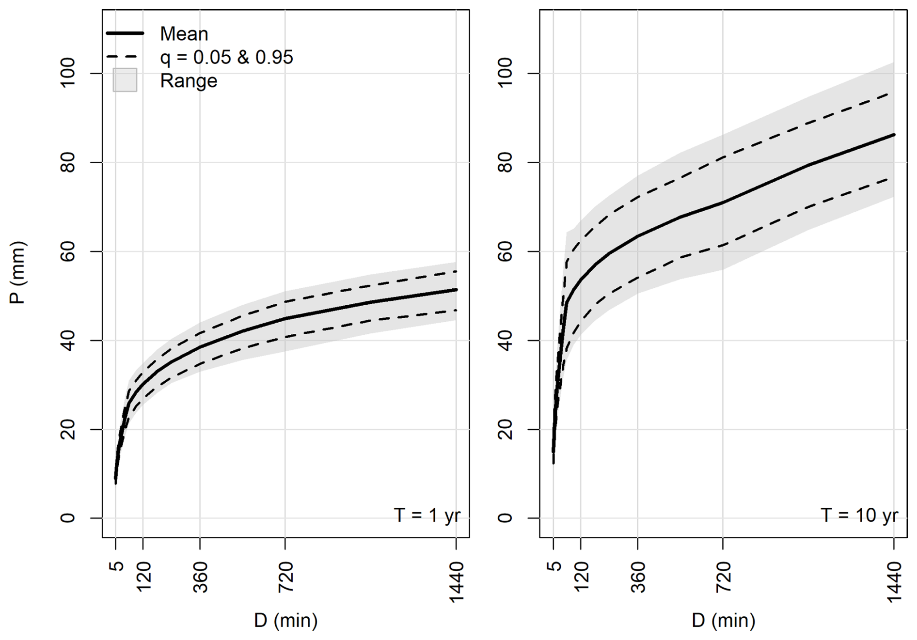
Figure 2 Precipitation amount-duration curves of point precipitation for return periods 1 year (left) and 10 years (right) based on the station data for the whole year. The solid curves represent the arithmetic mean over all 142 stations at each duration, averaged over the whole region. Range refers to the whole precipitation amount extent for each duration, while dashed lines refer to the quantiles 0.05 and 0.95.

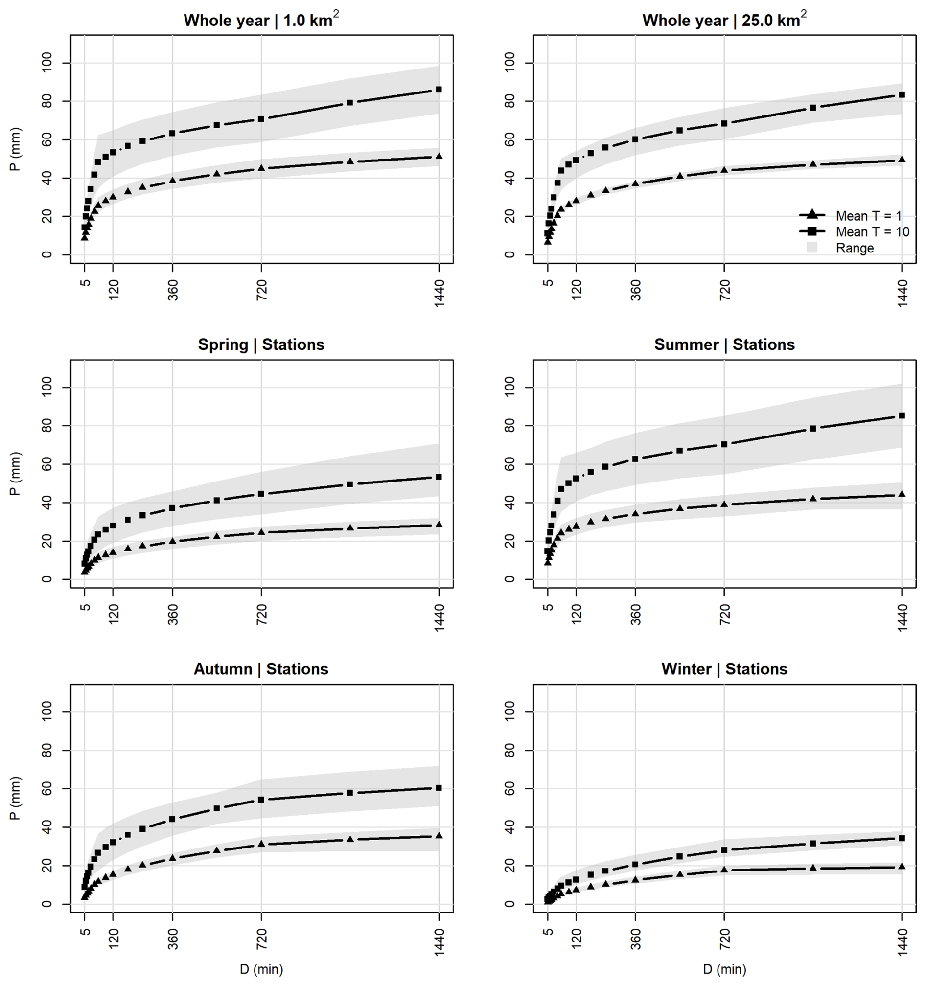
Figure 3 Mean and range of areal precipitation extreme values for 1 and 25 km² (top row). Mean and range of point precipitation extreme values or different seasons (center and bottom row).

Figure 3 the two bottom rows show the mean values of seasonal point extreme precipitation for the return periods of 1 and 10 years. For all seasons, the expected pattern of increasing precipitation with increasing duration is evident. The mean precipitation depth also increases with higher return periods. Additionally, the range of values (distance between minimum and maximum of precipitation amount for each duration) increases with the return period across all seasons. The progression of the mean values differs between seasons. In spring, autumn and winter, the slope decreases for all return periods for durations longer than 720 min compared to durations shorter than 720 min. However, it increases slightly in summer due to higher precipitation amounts, associated with longer durations and higher return periods in comparison to other seasons. For T = 10 years and D = 24 h, values of 85 mm are reached in summer, compared to 34 mm in winter. The lowest precipitation depths occur in winter, where the mean precipitation for T = 1 year and D = 24 h is only 19 mm. The range indicates that during summer, this combination of return period and duration occasionally results in maximum values exceeding 100 mm. Additionally, the range of precipitation depth is considerably smaller in winter.

The top row panels in Fig. 3 show the mean precipitation values for two areas of 1 and 25 km² for the whole year. As the area increases, the precipitation amounts decrease for the same return period and duration. For example, for T = 1 year and D = 24 h, the precipitation amounts are 34.2 mm for 1 km², but only 31.3 mm for 25 km². This behaviour confirms the decrease of precipitation amounts with increasing area size for the same return periods and durations as identified by e.g., Asquith and Famiglietti (2000). The range increases with return period for areal extreme values, while the range decreases as the area increases. The decrease in range with area is primarily due to the decreasing number of time series available for analysis as the area grows. The increase of extreme precipitation depth with duration and return period is evident here as well. Additionally, the range of values increases with higher return periods.

4.2 Areal Reduction Factors

Figure 4 presents an example of the yearly ARF values for D = 60 min and T = 10 years. The ARF increases with increasing area, and so does its range. It is observed that the mean and the median of the ARF values are almost identically, with values below 1, and both decrease with increasing area. For areas larger than 200 km², the mean and median values show a slight increase, which can be attributed to the small sample size, since as the area size increases, the number of areal time series decreases, e.g. only two time series are available for areas of 225 km². Additionally, the ARF range increases up to an area size of approximately 15 km² and stagnates or decreases for larger areas. Therefore, the largest ARFs are associated with an area size of roughly 15 km² and are very likely attributable to isolated outliers, as the 95th quantile does not show a significant increase at this area. The inter-quantile-range (IQR) as distance between q = 0.95 and q = 0.05 increases with increasing area, but only slightly compared to the total range, and starts to decrease for areas larger than 90 km². Overall, the deviation of outliers from the mean appears to be more significant in the upper bound than the lower bound in all cases, as indicated by the range and the IQR depicted in Fig. 4. As mentioned above, the sample size for areas larger than 81 km² is notably small and leads to high uncertainty in the results. Therefore, from this point on, the analysis will be limited to area sizes up to 81 km².

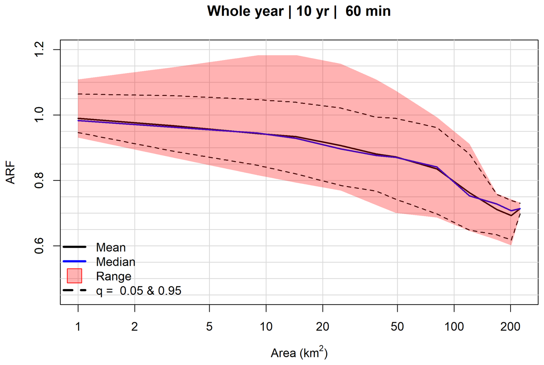
Figure 4 ARF values of the whole year time series, for events D = 60 min and T = 10 years. Range refers to the whole ARF extent for each duration, while dashed lines refer to the quantiles 0.05 and 0.95.

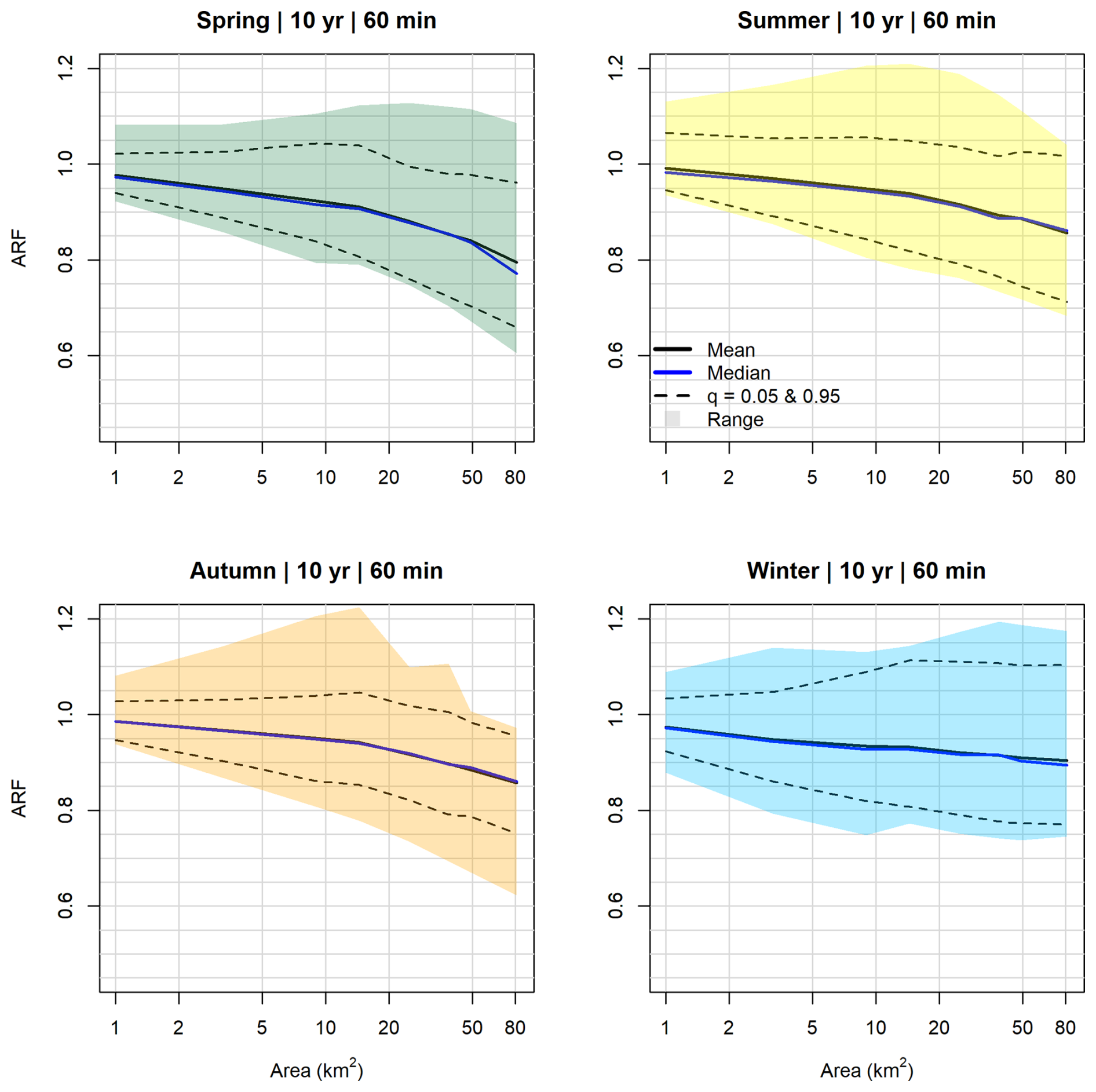
Figure 5 ARF values for seasonal time series, D = 60 min and T = 10 years. Range refers to the whole ARF extent for each duration, while dashed lines refer to the quantiles 0.05 and 0.95.

Figure 5 presents the seasonal ARFs for a duration of 60 min at a return period of 10 years. The smallest ARF values observed belong to spring, while the largest values occur in winter. The slopes of the mean and median of the winter ARF are both noticeably constant over area sizes. For all seasons, the range of ARF increases with area size, while in autumn, the range shows a more irregular pattern of increase and decrease. Cases of ARF>1 are identified in all seasons, where in spring, summer and autumn such values belong almost exclusively to the upper 5 % of the sample, probably indicating outliers. However, in winter, a noticeable part of the ARF values which fall into the IQR are higher than 1.

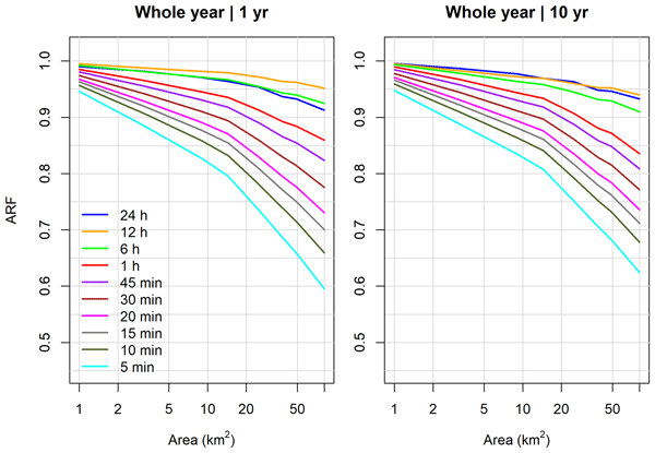
Figure 6 depicts ARFs for the entire year, different duration and different return periods. For ease of communication, only 10 of the 16 durations are displayed in these plots. For all return periods, the ARF increases with increasing durations and decreases with increasing area. An exception is the duration D = 24 h, which occasionally exhibits lower ARFs compared to the D = 6 h and D = 12 h (observed across all return periods). The 5 min duration has the lowest ARFs, with the smallest value 0.595 occurring at a return period of 1 year. The generally higher values of ARF for the return period of 10 years indicates the increase of ARF with increasing return period. This behavior is clearly demonstrated for durations between 5 to 20 min. In contrast, the ARF decreases with return period at durations between 60 min to 12 h for areas exceeding 9 km². The durations in between 30 and 45 min show no clear behaviour in this regard. Overall, the ARF curves appear to converge as the area decreases, meaning the ARF increases with area and approximates the value of 1. The exact ARF values for the entire year analysis are provided in the Table 1 for the return periods of 1, 2, 5 and 10 years.

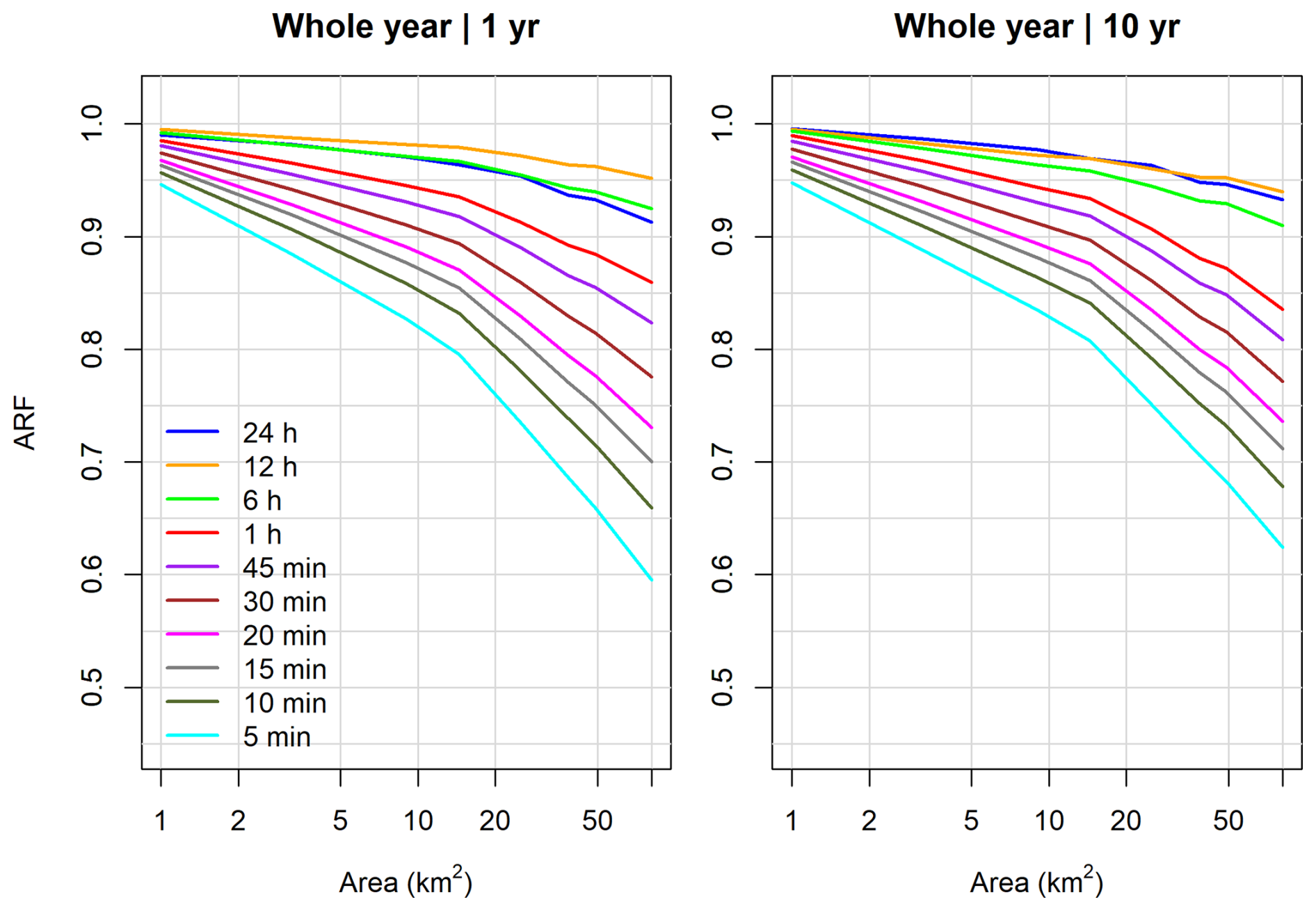
Figure 6 Mean ARF values over all raster cells of whole year time series, multiple durations and T = 1 and 10 years.

Table 1 ARF for different return periods, areas and durations.

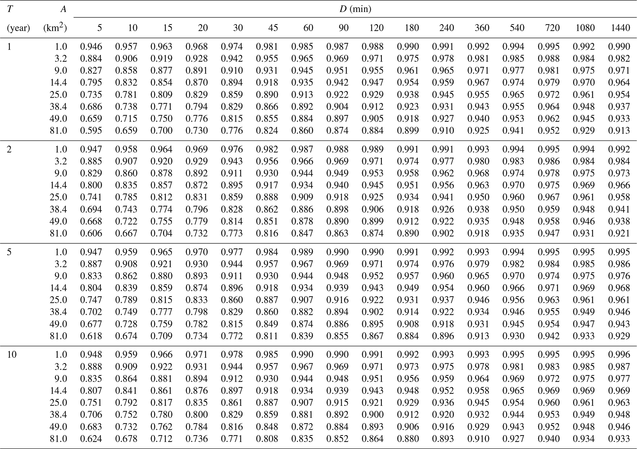
The difference between the ARFs between 1 and 10 years return periods is the largest at 5 min duration and 81 km². This indicates that the greatest discrepancy in ARFs is between different return periods. Since all other differences are smaller, it is concluded that the changes in ARF are more pronounced for smaller durations and larger areas.

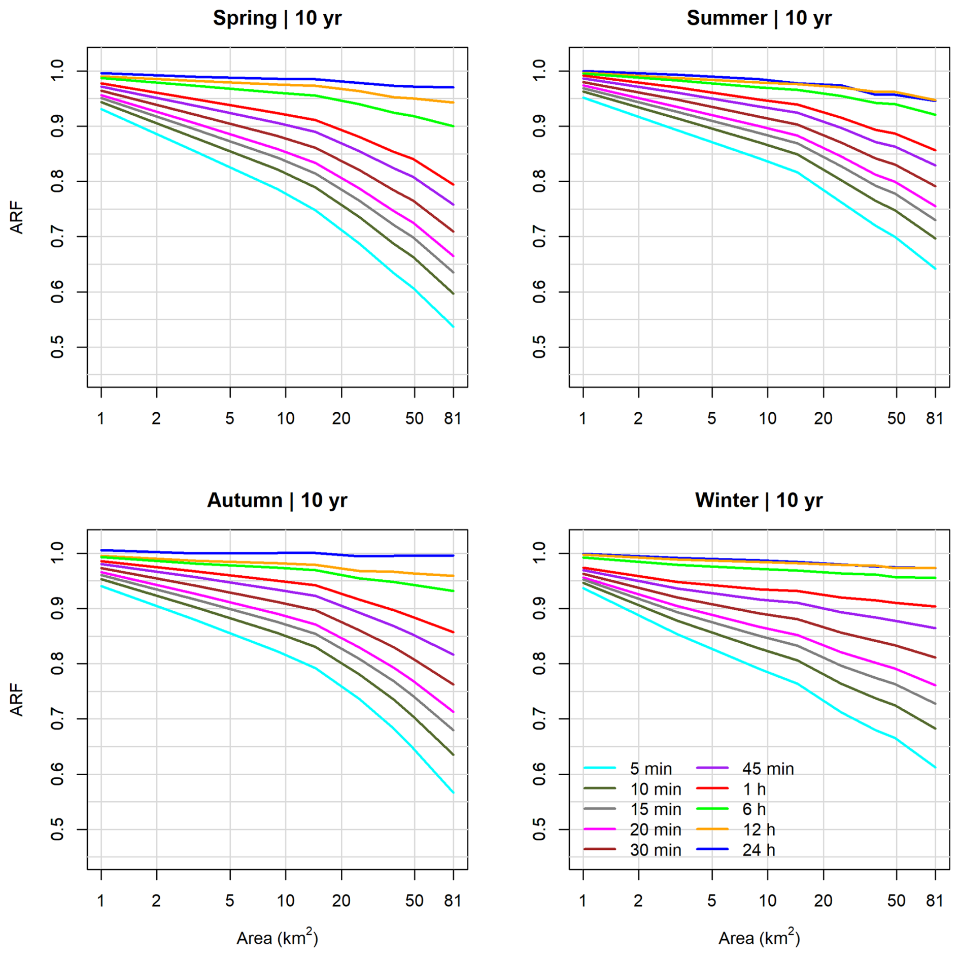
Figure 7 Mean ARF values over all raster cells of seasonal time series, multiple durations and T = 10 years.

Figure 7 presents ARF values separately for each season for T = 1 year. The same pattern of increase with duration and decrease with area size is detectable in all seasons. Winter exhibits the highest ARF values across most durations. In contrast, spring shows the lowest ARF values, particularly for shorter durations, specifically up to 6 h. The minimum ARF value is 0.497 for the duration of 5 min and an area size of 81 km². Summer and autumn show intermediate values which fall between those of spring and winter. In summary, seasonal variations are most prominent in the shorter durations (up to 6 h) and smaller areas.

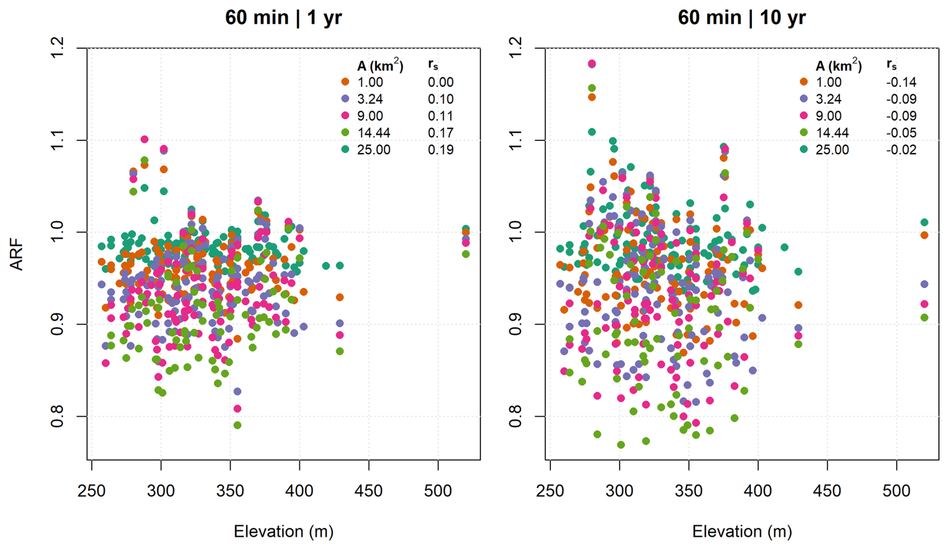
Figure 8 Elevation dependence of ARF values of whole time series, D = 1 h and T = 1 and 10 years.

To analyze the relationship of the ARF with the topography, the Spearman correlation coefficient (r_s) is calculated between the ARF values and the elevation of the stations for different area sizes, durations and return periods. Figure 8 shows the correlation between ARF and elevation for the area sizes of 1 to 25 km². The value of the correlation coefficients is also presented in the two plots. It is clearly noticeable that there is a low correlation between the ARF and the elevations. For the duration of 60 min and the return period of 1 year r_s spans between 0 and 0.19, increasing with area. For the same duration, as the return period increases to 10 years, the r_s values decrease and show a negative correlation between ARF and elevation, ranging from −0.14 for 1 km² and −0.02 for 25 km². It is noteworthy that the correlation decreases with increasing area for T = 10 years.

5 Discussion

In this section, the results are discussed in detail and compared with the literature. The ARF is analysed for its dependence on area size, duration, return period, season, and topography. Since all results are obtained for a dense network, but with limited spatial extent, the transferability of the results to other regions, especially under different climatic conditions, should be proven critically.

5.1 Area

Evidently, in all cases, across all durations and seasons, the ARF reduces with area, which complies with the definitions and findings among the related literature (Skaugen, 1997; Allen and DeGaetano, 2005; Breinl et al., 2020; Flammini et al., 2022). ARF decreases more rapidly with area for shorter durations, as in Breinl et al. (2020). This behavior can be attributed to the different types of precipitation events associated with various durations. Short-duration events generally exhibit higher spatial variability compared to long-duration events (Mineo et al., 2018). As the mean ARF is in most of the cases below 1, this study underlines the necessity for reducing point design values for determining the areal design storm. The largest reduction for a 1 km² area occurs in spring at a return period of 1 year, with an ARF of 0.928, corresponding to a 7.2 % reduction in areal precipitation. However, it is noteworthy that across seasons and return periods, values above 1 appear, which are in the upper 5 % of the extreme and contradicts the base assumption of the reduction of precipitation in ARF. Goshtasbpour and Haberlandt (2025) discuss this vastly in their study, where they attribute an increase in areal precipitation with increasing area (meaning ARF > 1), to the shortcomings of the sparse measurement networks and the conventional fixed-area spatial sampling methods. It is important to acknowledge that even with a dense network like WegenerNet, there are still events whose center of highest precipitation depth cannot be detected with the conventional sampling approaches, as Goshtasbpour and Haberlandt (2025) discuss. Furthermore, our results show that the assumption of approximation of the point extreme precipitation value, even with the areal extreme of 1 km² (Verworn and Schmidtke, 2006; Vaes et al., 2005) is not accurate and will lead to the overestimation in infrastructure planning. Widely used guidelines like DWA (2012) suggest that point precipitation can represent the areal precipitation of catchments up to 25 km², with an intentional overestimation for planning purposes. However, applying this assumption for an area of 25 km² at a duration of D = 5 min would result in a 26.5 % overestimation of areal precipitation, which seems excessive as a safety margin. Especially, when summed up with other safety margins resulting from conservative estimations, as, e.g., using the same return period for all durations within one design event (Cache et al., 2025). Without the application of ARF for small areas, overestimation of the urban drainage infrastructure dimensions is a significant risk.

5.2 Duration

As widely documented in the literature (Ramos et al., 2005; Barbero et al., 2014; Mineo et al., 2018; Breinl et al., 2020) the ARF has a direct relationship with duration in general. However, it is observed in this study that the ARF of the two longest durations, 18 and 24 h, does not follow the expectations. This irregularity is shown in Figs. 6 and 7 for the duration of 24 h. For the whole year results, for T = 1 year this behavior is observable for almost all area sizes, whereas for T = 10 years this happens only for areas larger than 25 km². The seasonal analysis show this pattern only in summer and winter for T = 10 years. Precipitation events with extensive spatial coverage may influence the statistics at these durations, extending well beyond the study area. Such regional-scale events may not be fully captured in the data, leading to these deviations.

5.3 Return Period

The four return periods analyzed exhibit varying effects on ARF, with the strongest impact observed in winter, where the largest differences between ARFs at T = 1 and 10 years occur. For the whole year, the smallest ARF was found at the smallest return period T = 1 year, contradicting literature findings (Allen and DeGaetano, 2005; Asquith and Famiglietti, 2000; Breinl et al., 2020), which generally report smaller ARF values for larger return periods. This deviation can be explained by the distinct behavior of short-duration events, where areal precipitation increases more significantly with increasing return periods than point precipitation. The spatial variability of the short-duration precipitation events decreases with increasing return periods. An example of similar behavior of ARF for short durations across different return periods could not be found in the literature. This can be caused by the rarity of such a data set: the spatial and temporal high-resolution station-based data set from WegenerNet appears to be one of only a few data sets existing globally, and it is the first data set of this kind used to estimate ARFs. Again, due to the limited study area it remains unclear, if this finding represents rather a general behaviour or an observational-scale effect, or if it is related to the regional climate. Verworn and Schmidtke (2006) determined ARF using an almost identical method and concluded the influence of return periods to be minimal, and suggested that the return period can be disregarded in the ARF calculation. However, based on the differing ARFs observed in this study as a function of return periods, as well as the distinct behavior of short durations with increasing return periods, the influence of return periods on ARF cannot be neglected.

5.4 Seasons

The dependence of ARF on seasons, as identified by Allen and DeGaetano (2005), was partially confirmed in this study. Allen and DeGaetano (2005) found that the ARF in warm seasons (April–September) has lower values compared to those of the cold seasons (October–March). This pattern is confirmed in this study, particularly for the shorter return periods. The smallest ARFs are observed in spring and summer, which can be attributed to the predominant convective precipitation events. These events exhibit high spatial variability (Corradini et al., 2022), which leads to smaller ARF values as the area size increases. The autumn ARF values show a very similar mean and median to those of summer. However, the largest ARF values belong to autumn when looking at the range of the values (Fig. 5). In contrast, winter shows higher values on average. While the dependence on seasons can be identified, the combined effects of return periods and duration complicate definitive conclusions, such as those made by Allen and DeGaetano (2005). A deeper insight could be achieved by multifractal analysis of the scaling behavior as done by Veneziano and Langousis (2005), but is beyond the scope of this study.

5.5 Topography

As the correlations showed in Fig. 8 in this study, an insignificant relationship between the ARF and the elevation is observed. Although the correlation increases with area for shorter return periods, even the strongest correlations do not reach the value of 0.2, which indicates a weak relationship with elevation. Ghaemi et al. (2021) found no significant relationship between extreme precipitation and elevation for WegenerNet stations either. It is interesting to note that ARF show no correlation with elevation, since extreme values themselves show clear dependencies (see e.g. Marra et al., 2021 and references within). However, it should also be noted that the spatial interpolation of precipitation for the WegenerNet was conducted without accounting for elevation, which was justified by the relatively small elevation variation among the climate stations (Kabas et al., 2011). As a result, the areal precipitation between stations may not have been accurately interpolated, which must be considered when interpreting the results of this analysis.

6 Conclusions

In this study, ARFs were determined using a fixed-area method from high-resolution spatial precipitation data from WegenerNet for the Feldbach region in Austria. The WegenerNet data offer the advantage of capturing the spatial variability of the precipitation in the region more accurately than the data sets used by previous studies. Subsequently, the ARFs were analyzed for their dependence on area size, duration, return period, seasons and topography. The main findings are:

• ARF, in most cases, decreases with the return period, except for the sub-hourly durations. For events with durations shorter than 1 h, the ARF partially increases with the return period, which was found for the first time and disagrees with the findings from the current literature on this topic (Asquith and Famiglietti, 2000; Allen and DeGaetano, 2005; Breinl et al., 2020). These differences can be explained by the improved representation of the spatial variability due to the high-resolution data. Further investigations using comparably high-resolution data in other regions are recommended to confirm this finding.

• The ARF for the durations 1, 3, 6 and 12 h confirm values from the literature despite the significant increase in the spatial resolution. This conclusion applies for ARFs based on time series for whole years not accounting for seasons.

• ARF increases with increasing duration (including sub-hourly durations).

• Application of ARF is necessary for areas as small as 1 km², questioning results from the literature (Vaes et al., 2005; Verworn and Schmidtke, 2006), which implies that pixel-wise precipitation estimates like radar or satellite cannot be considered equivalent as point measurements.

• The correlation between the ARF and elevation was found to be insignificant. However, the elevation differences among the WegenerNet stations are relatively small and thus might not lead to marked patterns.

Due to the limited spatial extent of the studied network, the transferability of the results to other regions, especially under different climatic conditions, should be proven critically.

We recommend further investigations using comparable high-resolution data set in other regions and for larger networks if available, as well as using different methods of fixed-area ARF calculations on the same data set.

Appendix A: Validation of the fitted exponential distribution function

For the DAF estimation precipitation quantiles of different return periods are required. An exponential distribution is fitted to the peak-over-threshold series (POT), consisting of the highest 40 extreme events of each time series for each duration (see Sect. 3.1.1).

In Fig. A1, for the two rain gauges closest to the raster centre of the Feldbach raster field, the observed extreme values of the POT are shown together with the fitted distribution function and the ÖKOSTRA design values. While for D = 5 min an overall good fit is visible, for D = 1 h a slight underestimation for return periods 2 years < T < 5 years can be identified. However, the fitted distribution function represent the observed extreme values better than the ÖKOSTRA values for D = 1 h, which underestimate the precipitation quantiles. This indicates the need of spatial dense networks for a robust extreme values estimation.

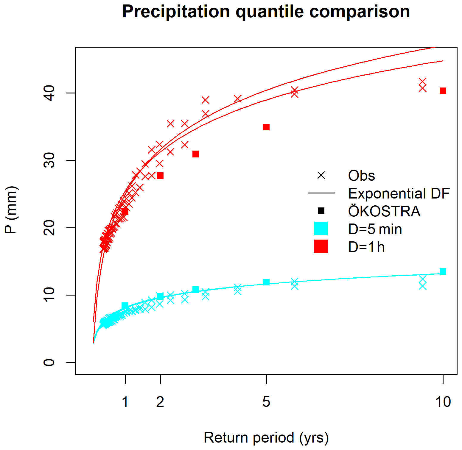
Figure A1 Observed extreme values (Obs) and fitted distribution functions (Exponential DF) for two precipitation gauges in the Feldbach raster field, along with the ÖKOSTRA design values for D = 5 min and D = 1 h (entry 5433 in the eHYD catalogue).

An overestimation for T > 6 years is identified for D = 1 h as well. This overestimation is attributed to the shortness of the time series with 15 years, which allows only an uncertain estimation of precipitation quantiles for return periods larger than one-third of the time series length.

In Fig. A2, for three raster fields within the Feldbach raster the observed precipitation amounts for areas of A=1, 25, 81 km² and the precipitation quantiles from the fitted exponential distribution functions are shown. For none of the studied areas a systematic underestimation or overestimation can be identified.

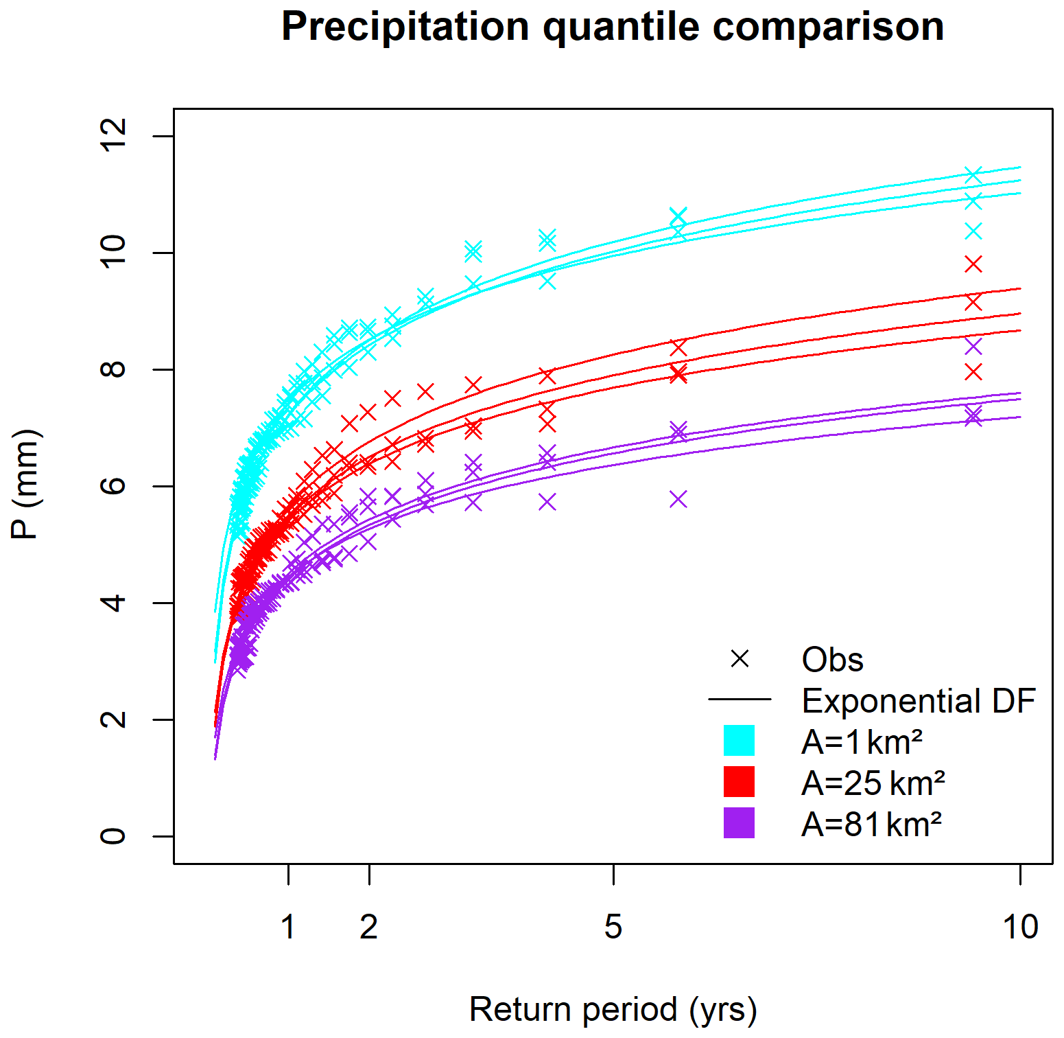
Figure A2 Observed extreme values (Obs) and fitted distribution functions (Exponential DF) for three raster fields within the Feldbach raster for A=1, 25, 81 km² for D = 5 min.

It could further be questioned if interpretations of return periods up to 10 years are valid by an observation period of in total 15 years only. For a very large sample size (e.g., 100 years) a robust conclusion could be drawn via bootstrapping by first drawing multiple times randomly 15 years (without putting them back), followed by an extreme value analysis of each so-created subset and finally compare the resulting precipitation quantiles for different return periods. Unfortunately, given the small sample size of 15 years only, this approach was modified as follows.

The bootstrapping was carried out 100 times, sampling from the available 40 extreme values observed within the 15 years, but with replacement to avoid the influence of smaller sample sizes for the extreme value analysis. An exponential distribution function was fitted to each subset. The deviations of the precipitation quantiles PQ of the single realisations are considered as rE (relative error) from the arithmetic mean of all realisations, and are quantified for each return period T (Eq. A1) and shown in Fig. A3:

$$\begin{array}{}\text{(A1)}& \mathrm{rE}\left(T\right)=\sum _{i=\mathrm{1}}^{\mathrm{100}}{\displaystyle \frac{\left({\mathrm{PQ}}_i\left(T\right)-\stackrel{\mathrm{‾}}{\mathrm{PQ}\left(T\right)}\right)}{\stackrel{\mathrm{‾}}{\mathrm{PQ}\left(T\right)}}}\end{array}$$

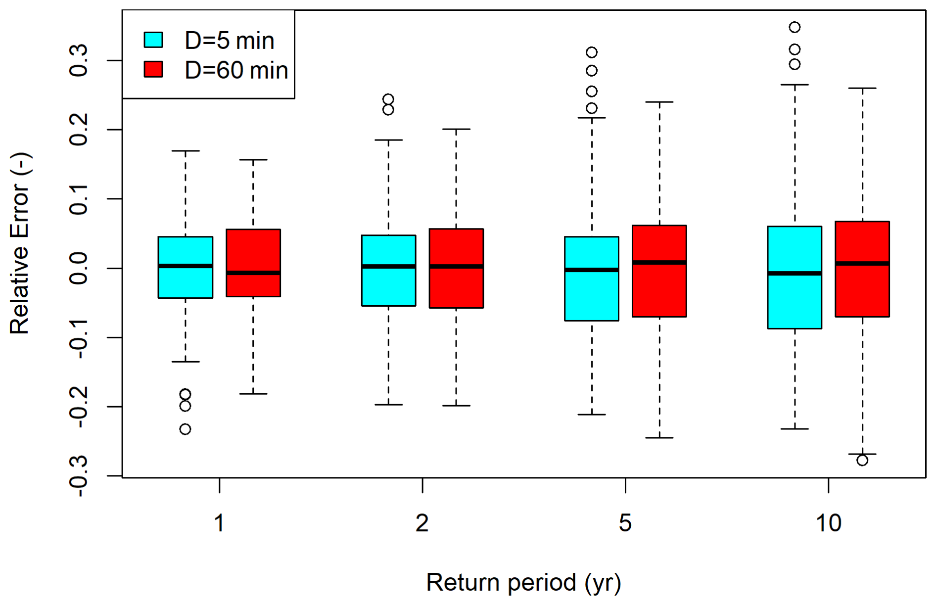
Figure A3 Deviations of the precipitation quantiles of the single realisations considered as relative error in dependence of the return period (for station 58).

It can be seen that changes of median and the second and third quartile of rE from T = 5 years to T = 10 years are small, so the analysis of the results for T = 10 years is as legitimate as results for T = 5 years. However, percentiles of 5 % and 95 % are increasing slightly, which is a direct impact of the chosen approach, since some realisations contain the highest (or lowest, respectively) extreme value of the sample size multiple times.