Spatial machine learning modelling reveals that soil indicators and tree type best explain shallow landslide release

The exploration of shallow landslide susceptibility is often impaired by biased landslide inventories, and by over-optimistic performance metrics linked to inadequate models. Here, we use a systematically mapped event inventory of 571 shallow landslides triggered in southern Norway and apply 32 gradient boosted decision tree models to rigorously test the effects of (1) a nested vs. simple cross-validation strategy, (2) spatial vs. non-spatial models, (3) four different cross-validation sampling strategies which were applied on (4) full vs. forest-only datasets. Model evaluation shows that models with random cross-validation provided the highest test performance metrics but did not account for autocorrelation and were likely over-optimistic. The spatial models with spatial cross-validation reduced autocorrelation in the model residuals at the expense of predictive power. Although no model emerged as optimal, findings across models suggest that important explanatory factors like elevation, aspect and bedrock weatherability serve as soil indicators, illustrating a need for improved datasets for soil thickness and heterogeneity. In the forest-only models, tree type was consistently an important predictor, with higher landslide susceptibility in deciduous forest, illustrating the potential of forest variables and forest-specific threshold values in shallow landslide susceptibility mapping.

1 Introduction

Rainfall-induced shallow landslides pose a significant and escalating threat to societies worldwide. In this study, we define shallow landslides as gravitational mass movements of the slide and flow type involving soft, surficial material at rooting depth; this includes debris slides, debris avalanches, debris flows and debris floods (Hungr et al., 2014). Shallow landslides can be triggered seismically during earthquakes, anthropogenically due to deforestation and construction, by rockfalls as well as a rise in porewater pressure by rainfall and/or snow melt. The majority of shallow landslides are, however, rainfall-triggered (Haque et al., 2016; Sultana, 2020; Sim et al., 2022). Under future climate scenarios, an increase in frequency and magnitude of heavy precipitation over mid-latitude and tropical mountainous areas will likely lead to more rainfall-induced shallow landslide events (Crozier, 2010; Jakob and Owen, 2021; Stoffel et al., 2014; Gariano and Guzzetti, 2022). Future shallow landslide hazard assessments will thus require the inclusion of rainfall variables in dynamic models (Moreno et al., 2025; Steger et al., 2024) to predict when landslides will occur as well as improved static models to predict where landslides will occur.

Studies of shallow landslide susceptibility are commonly differentiated into knowledge-driven, physically based and data-driven methods; all of which use landslide inventory data for validation, while only the data-driven method also applies this data as input (Corominas et al., 2014). The current Norwegian susceptibility map can be classified as a knowledge-driven approach because landslide inventories are only used for validation, while shallow landslide starting points are determined based on expert considerations of suitable threshold values for slope, planar curvature and upstream catchment area, and subsequent runout modelling (Fischer et al., 2012; Pullarello et al., 2025). Physically based methods simulate the processes on single slopes to small regions, incorporating hydrological processes, soil mechanics and topography (Sorbino et al., 2010). Approaches under this category can be placed on a continuum between steady-state models, guilty of oversimplification, and sophisticated numerical models, which are computationally expensive, and depend on detailed, often unavailable hydrometeorological and soil data (Sachinthaka et al., 2025; Ye et al., 2025). Data-driven approaches build on the assumption that combinations of topographic, geological and meteorological factors that have triggered shallow landslides in the past can be used to make quantitative predictions of future susceptibility to shallow landslides (Corominas et al., 2014). While data-driven approaches can be regarded as the standard method for regional or even national susceptibility mapping, they do not account for the complex physical mechanisms behind shallow landslide release, and tend to suffer from limited and biased datasets (Lima et al., 2022). More recently, attempts have also been made to combine data-driven and physically based approaches, potentially overcoming weaknesses of both methods (Han and Semnani, 2025; Ye et al., 2025).

Among the data-driven models, machine learning methods have received exponentially growing attention over the last 10 years and often outperform more classical statistical approaches as they are better suited to tackle non-linear relationships, high dimensionality and collinearity among predictors (Ye et al., 2025). In particular, gradient boosting decision tree methods have received a lot of attention due to their predictive performance (Cao et al., 2020; Wei et al., 2022), and many recent studies report almost perfect levels of landslide prediction accuracy (Choubin et al., 2025; Dai and Huang, 2025; Liu et al., 2021). However, in line with earlier work (Steger et al., 2021; Lima et al., 2021), we suggest that these are often overly optimistic reports which are almost certainly the result of model overfitting, and that the popularity and perceived ease of use of these methods require a robust set of standardised best practice protocols (Reichenbach et al., 2018; Lombardo and Mai, 2018; Schlögl et al., 2025). Decision tree models for classification of binary outcomes, e.g. the occurrence of shallow landslides, are powerful algorithms but predictive accuracy and the importance of predictors are susceptible to several choices made by the researcher (Hastie et al., 2009; Probst et al., 2019). So-called hyperparameters control aspects such as model complexity, regularisation strength (the degree to which a model overfitting is constrained) and decision tree structure (the depth and complexity of decision trees used in the model). Hyperparameters including learning rate, number of trees and maximum tree depth can be either chosen by default, set by the researcher, or selected following a wide range of available data-dependent optimisation procedures (Probst et al., 2019).

Typically, the optimisation process involves a resampling technique such as cross-validation (CV; Bischl et al., 2012), but CV is sensitive to how folds are constructed. For example, in random CV, the data are randomly assigned to k-folds and the optimisation process repeatedly selects a different fold as a test set, leaving the remainder as training set and evaluates model performance for each hyperparameter combination across multiple train-test splits. However, to account for spatial autocorrelation in geospatial data, spatial strategies of fold assignment may be better suited (Brenning, 2012). Specifically, in some ecological machine learning applications with spatially dependent data spatial cross-validation approaches have been found to be more appropriate and less likely to lead to overly optimistic results (Linnenbrink et al., 2023; Meyer and Pebesma, 2022; Schratz et al., 2019). In spatial CV, the folds are assigned to spatial clusters or blocks, the size and clustering of which can also be set, and cross-validation proceeds in the same way while accounting for some of the spatial autocorrelation in input data (Meyer et al., 2026). As shallow landslides typically occur in spatial clusters and inventories often exhibit a fractal structure (Ghosh et al., 2012; Liu et al., 2019; Rouai and Jaaidi, 2003), it is highly likely that landslide data exhibit spatial autocorrelation, suggesting that spatial CV is an appropriate option for both hyperparameter optimisation and model evaluation. The importance of spatial CV in landslide susceptibility studies has been advocated elsewhere (Brenning, 2005; Goetz et al., 2015b; Knevels et al., 2023; Petschko et al., 2014; Schlögl et al., 2025), and it has also been shown that failure to account for spatial autocorrelation during both hyperparameter optimisation and model evaluation can lead to overfitting and inflated performance estimates that do not generalise to new spatial locations (Steger et al., 2016). Nonetheless, many recent shallow landslide susceptibility studies appear to apply random or no CV methods (e.g. Choubin et al., 2025; Li et al., 2025; Utthasini et al., 2026; Wang and Deng, 2025; Qin et al., 2025) and potentially fail to consider the inherent spatial relationship of shallow landslide inventories.

Another source of potential over-optimism in landslide susceptibility models is that, apart from a recent study which incorporates spatial structure in a Generalised Additive Modelling approach (Knevels et al., 2023), the inherent spatial structure in landslide datasets is rarely modelled directly. In some cases, spatial structure may be sufficiently addressed by spatial CV, or directly in models by the inclusion of spatially explicit variables such as initiation point coordinates or distances to land features such as rivers, roads or settlements (e.g. Choubin et al., 2025; Qin et al., 2025; Steger et al., 2016, 2021). However, landslide susceptibility studies rarely test for spatial autocorrelation in model residuals to ensure that the spatial structure has been accounted for. If spatial structure remains in model predictions, the results may be over-optimistic, suffer from low generalisability, or both (Mets et al., 2017; Roberts et al., 2017). In this paper, we address the above issues by utilising the Gaussian Process Gradient Boosting algorithm, which is an extreme gradient boosting machine learning method that allows for the addition of random effects in the model (Sigrist, 2022). Utilising this approach, together with nested spatial cross-validation and testing for residual spatial autocorrelation and other statistical artefacts, our first objective (O1) was to demonstrate the potential to address overfitting in landslide modelling with machine learning methods.

The modelling procedure is applied to a landslide dataset related to an extreme rainstorm event in Norway in 2023. As the shallow landslides all occurred within a period of two to three days, the dataset is not subject to another form of uncertainty, temporal heterogeneity, which tends to affect landslide inventory data (Reichenbach et al., 2018; Ye et al., 2025). Being based on an event-inventory and including event-specific hydrometeorological variables, results from this study offer limited generalisability and a shallow landslide susceptibility map has therefore not been produced. Nevertheless, the dataset provides a unique opportunity to explore shallow landslide explanatory factors based on an inventory with a consistent and systematic mapping routine (Rüther et al., 2024), thus minimising geographic bias. Hence, our second objective (O2) was to analyse morphological, geological and hydrometeorological variables relevant to shallow landslide release based on gradient boosted models on the full dataset.

Moreover, the impact of forest cover and characteristics were studied based on additional gradient boosted models applied to a sub-dataset consisting of shallow landslide and control points in the forest. The effects of vegetation and trees on slope stability are relatively well studied on the scale of single trees and tree stands (e.g. Kim et al., 2017; Schwarz et al., 2010a, b) and on the scale of forested slopes in physically based models (e.g. Jiang et al., 2023; Kim et al., 2020; Medina et al., 2021; Spiekermann et al., 2023). However, examples of data-driven shallow landslide susceptibility studies which consider vegetational or forest variables beyond landuse are more rare (Moos et al., 2016; Goetz et al., 2015a; Spiekermann et al., 2022, 2023). Therefore, by repeating our model routine based on a sub-dataset from forested sites, our third objective (O3) was to demonstrate the important role of forest characteristics in influencing landslide susceptibility.

2 “Hans” event and shallow landslide inventory

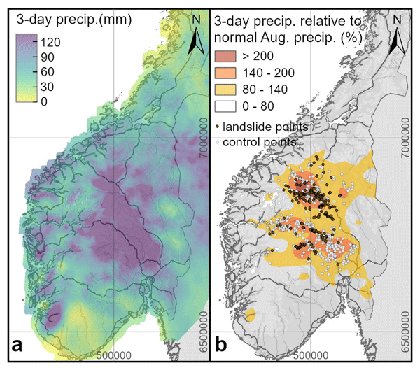
On 7–9 August 2023 southern Norway was hit by the extreme rainstorm event “Hans”, a powerful storm which originated as two low-pressure systems that merged over the European continent and subsequently approached Norway from the southeast. This is unusual as most low-pressure systems affecting southern Norway have a westerly origin. Consequently, large areas in southeastern Norway (20 600 km²) which are normally situated in the rain shadow, received 70–100 mm of rain in 24 h, corresponding to rainfall with a 100 year return period (Granerød et al., 2023). While the total accumulated precipitation during the “Hans” storm exceeded 110 mm in southeastern as well as some western areas (Fig. 1a), “Hans” precipitation during these three days surpassed 80 % of normal precipitation for the entire month of August in large parts of eastern Norway (Fig. 1b). The storm caused widespread flooding and numerous shallow landslides with severe impacts on infrastructure, damage to private property and disruption to major transport routes. No lives were lost, partly due to well-functioning early warning and evacuation of around 4600 individuals (DSB, 2024). The “Hans” storm is amongst the most expensive natural disasters in Norway with direct cost estimated to USD 0.7 billion (Meld. St. 27, 2023–2024).

Shallow landslides triggered during this storm were systematically mapped based on the dNDVI (differential Normalised Difference Vegetation Index) calculated for composite pre- and post-event satellite images with 10 m spatial resolution (Rüther et al., 2024). The mapping was validated with all available data sources including satellite images with 3 m spatial resolution (29 % of mapped landslides), post-event orthophotos (54 % of mapped landslides), as well as drone footage and/or field observations (17 % of mapped landslides). The inventory data is differentiated into debris slides (smallest events for which no flow behaviour was detectable), debris flows (well-defined release area and inferred flow behaviour, including debris avalanches) and debris floods (initiated due to continued riverbed and riverbank erosion). Debris floods were distinguished from debris flows and avalanches both sedimentologically, based on sorting of deposits, and geomorphologically due to lack of levees (Bondevik and Rüther, 2025). This approach is possible for landslides validated based on post-event orthophotos and field observations, while coarser geomorphological characteristics like channel proximity and slope angle were more decisive for landslides validated with satellite imagery. Compared to the Norwegian crowd-sourced landslide database (NSDB), the systematic mapping approach resulted in a 246 % increase in the number of detected shallow landslides (from 263–648) and a 35 % reduction of the spatial bias towards the road network for the occurrence of shallow landslides within 50 m of a road (from 61.6 % to 25.9 %; Rüther et al., 2024). The “Hans” shallow landslide inventory allows for the investigation of explanatory factors of a rare event compared to results based on multi-temporal inventories.

Figure 1 (a) 3 d cumulative precipitation from 7–10 August, 2023 (06:00 UTC or 8 a.m. local time) (b) cumulative precipitation shown in (a) relative to normal precipitation for the entire month of August (for the standard normal period 1991–2020), and position of landslide and control points. Topographic map: © Kartverket, SeNorge.

3 Data preparation

The data preparation consisted of editing of a published shallow landslides inventory (Rüther et al., 2024; Sect. 3.1), sampling of control or non-landslide points (Sect. 3.2) and the collection of attribute data to be included as explanatory factors (Sect. 3.3).

3.1 Landslide points

The machine learning supported analyses presented in this study are based on a refined version of the “Hans”-Landslide-dataset presented in Rüther et al. (2024). The original polygon dataset is mapped based on seamless, cloud-free greenest-pixel Sentinel-2 composites (Lindsay et al., 2022) together with additional data sources locally, including post-event orthophoto images, the NSDB database and field work by the main author. The published version of the dataset consists of 648 mapped polygons which were differentiated into 56 debris floods, 388 debris flows (including debris avalanches) and 204 debris slides. The refinement of the dataset included a re-evaluation of the placement of starting points, and a revisited differentiation into debris flows and debris floods assisted by all available data including slope angle. Inferred debris floods were then excluded from the point dataset because they belong to a different release process population than debris slides, flows and avalanches. While debris slides are initiated at the surface by continued riverbed and riverbank erosion (Church and Jakob, 2020), the latter have well-defined release areas in which failure occurs at shallow depth due to water infiltration, rise in porewater pressure and loss in shear strength (Bogaard and Greco, 2016). Many studies choose either the centroid points of mapped shallow landslide polygons (e.g. Ageenko et al., 2022; Arabameri et al., 2022) or sample distributed points throughout the landslide scars (e.g. Quevedo et al., 2022). Predictive capability of different susceptibility models has been shown to vary with different sampling strategies with distributed landslide scar points scoring highest (Dou et al., 2020). Yet, the model design has to match the intention of the study (Lima et al., 2023), and as we wish to investigate the influencing factors for shallow landslide release areas rather than their runout, the initiation points are the most appropriate landslide point sampling method. The shallow landslide point dataset (debris slides and debris flows, including debris avalanches) comprises 571 starting points released during the “Hans” storm.

3.2 Control points

In line with other studies in the field, the machine learning models are based on a similar amount of landslide and non-landslide or control points (Huang and Zhao, 2018; Wu et al., 2020), and 571 control points have been sampled based on the following workflow:

1. Selection of a large random sample of points (571 000) that are within the landslide point attribute ranges for elevation, slope and relative precipitation.

2. Normalisation of the three attributes relative to the maximum observed value for the landslide points. This means that all landslide and control points can be seen in a three-dimensional (3D) attribute space for elevation, slope and relative precipitation with values ranging from 0–1.

3. Find the 5710 closest non-landslide points in the normalised 3D attribute space and randomly select 571 (Figs. 1b and 2). Control points are hence relatively close to the elevation, slope and relative precipitation of a corresponding landslide point, but not necessarily the closest. Choosing only the closest point in the 3D attribute space will create control points that tend to be geographically close to the landslide point.

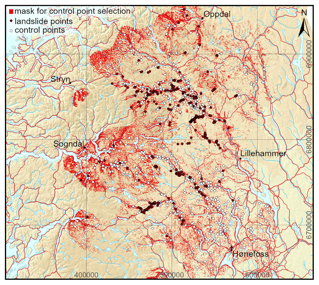
Figure 2 Shallow landslide starting points and control points together with the mask used for control point selection. © Kartverket.

Our control point sampling approach ensures parity in distribution across relative precipitation, slope and elevation (red areas in Fig. 2). This means that the contribution of these predictors is reduced to effects within the observed attribute ranges and will generally be lower than for approaches with completely randomised selection of non-landslide points (Dou et al., 2023). Controlling for elevation and slope jointly has a similar effect as masking trivial areas from the absence sampling area, e.g. the exclusion of certain landuse categories such as water bodies and glaciers (Schlögl et al., 2025). Moreover, as the influence of precipitation and slope on shallow landslide susceptibility is well established (Lima et al., 2022) and as relative precipitation was a key predictor in several of the tested Random Forest models in a recent master thesis (Peeters, 2024), our approach may force machine learning models to dive deeper into the effect of less obvious predictors.

3.3 Attributes considered as explanatory factors

The current national DEM (Digital Elevation Model) is predominantly based on lidar-data and is available in 1 and 10 m resolution. However, 54.5 % of Norway's landmasses were laser scanned with relatively low resolution (2 pt m⁻²) and 11.4 % are based on image-matching (kartverket.no). Therefore, the elevation accuracy in dense forest can be relatively poor and above the treeline, inaccuracies include severe elevation artefacts due to image-matching of glaciated and snow-covered areas. In addition, the 1 m DEM consists of one-pixel-wide holes at most project boundaries. This study is therefore based on a 5 m DEM produced by the Norwegian Geological Survey (NGU) where holes in the national DEM have been filled while the other weaknesses mentioned above have not been solved (Pullarello, 2024).

A series of morphological attributes are considered:

• (a)

  Elevation (m a.s.l.)

• (b)

  Slope (degrees)

• (c)

  Planar curvature

• (d)

  Profile curvature

• (e)

  Northerness (cosine of aspect)

• (f)

  Easterness (sine of aspect)

• (g)

  Landforms (based on the Topographic Position Index)

Elevation is the 5 m DEM provided by NGU (Pullarello, 2024) while all other morphological attributes are derived from the same DEM. To account for the circular nature of aspect values, northerness and easterness are considered in our machine learning models. The profile curvature describes the radius of curvature parallel to the direction of the steepest slope. Positive profile curvature values indicate that the surface is concave downslope leading to flow acceleration while negative values correspond to convex downslope surfaces and decelerating flow. The planar curvature describes the radius of curvature perpendicular to the direction of the maximum slope. Positive planar curvature values indicate that the surface is laterally convex causing divergent flow while negative values correspond to laterally concave surfaces and convergent flow. The Terrain Ruggedness Index (TRI) measures the topographic variation by calculating the elevation difference between each cell and its eight neighbours (Riley et al., 1999). While Gradient Boosting is more robust to multicollinearity than linear models, highly correlated predictors can still lead to instability and since TRI correlated strongly with slope, it was omitted from the final models. Topographic position has been analysed and landforms classified following the procedure suggested by Weiss (2001). The Topographic Position Index (TPI) compares the elevation of each cell in a DEM to the mean elevation of an annulus-shaped neighbourhood around that cell. TPI was calculated for small-scale neighbourhoods (TPI300 considering cells within 150 and 300 m radius) and for large-scale neighbourhoods (TPI2000 considering cells within 1850 and 2000 m radius). Building on TPI300 and TPI2000, landscapes were classified into discrete slope position classes and further into the following landforms (De Reu et al., 2013; Weiss, 2001): 1: canyons, 2: shallow valleys, 3: headwaters, 4: u-shaped valleys, 5: plains, 6: open slopes, 7: upper slopes, 8: hills in valleys, 9: midslope ridges and 10: high ridges. Due to low occurrences in many of the categories, the dataset was reclassified to open slope versus all other categories.

We further considered the following geological attributes with data provided by the Norwegian Geological Survey (NGU):

• (h)

  Bedrock weatherability $\mathrm{1}:\mathrm{50}\mathrm{000}-\mathrm{1}:\mathrm{250}\mathrm{000}$

• (i)

  Superficial deposits $\mathrm{1}:\mathrm{20}\mathrm{000}-\mathrm{1}:\mathrm{500}\mathrm{000}$

• (j)

  Deposit thickness $\mathrm{1}:\mathrm{20}\mathrm{000}-\mathrm{1}:\mathrm{500}\mathrm{000}$

The national bedrock map (NGU, 2025a) has 121 categories for the main bedrock type. These are reduced to five weatherability classes (see Table A1 in Appendix A for details) differentiating bedrock which weathers: 1: very easily (carbonous rocks), 2: easily (shale, phyllite), 3: relatively easily (mafic plutonic rocks), 4: slowly (sandstones, conglomerates, felsic volcanic rocks, i.e. granites, and metamorphic rocks, i.e. gneiss) and 5: very slowly (quartzite and quartz sandstones). The number of categories of the national Superficial deposits (NGU, 2025b) were also reduced (see Table A2 in Appendix A for details). The soil condition (“grunnforhold”) dataset provided by the Norwegian Institute of Bioeconomy Research (NIBIO) was also considered but excluded since it is not seamlessly available for the study area. In addition, the models include a deposit thickness map (NGU, 2025c) which considers three categories: 1: bare rock, 2: thin deposits (<0.5 m) and 3: thick deposits (>0.5 m). The bedrock, superficial deposits and deposit thickness maps are vector data compiled from datasets with highly variable scales (as specified above).

Moreover, we consider the following hydrological and meteorological attributes:

• (k)

  Flow accumulation (on logarithmic scale)

• (l)

  Groundwater (value for 7 August 2023 relative to normal for the same day)

• (m)

  Precipitation (acc. 3 d, mm)

• (n)

  Relative precipitation (acc. 3 d relative to normal August precipitation, %)

• (o)

  Maximum precipitation intensity (in mm/ 3 h)

Flow accumulation is calculated with the D8 flow modelling algorithm (O'Callaghan and Mark, 1984), and the maximum values in an area with 30 m radius surrounding landslide and control points are allocated. The Topographic Wetness Index (TWI) and the Stream Power Index (SPI) were also calculated (Saleem et al., 2019) but since both indices are derivatives of flow accumulation and slope, they naturally correlate strongly with these variables, and are excluded from the analysis. Pre-“Hans” relative groundwater level is the HBV-modelled groundwater for 7 August 2023 in mm relative to the 1981–2010 normal groundwater level for the same day and a spatial resolution of 1 km (Beldring et al., 2003; Bergström and Lindström, 2015). The total “Hans” precipitation is derived from seNorge v2018, a gridded observation-based dataset with 1 km spatial resolution and accumulated over three hydrological days (from 7 August 2023, 8 a.m.–10 August 2023, 8 a.m.). The relative precipitation is the accumulated precipitation for the above-mentioned “Hans” time period relative to normal precipitation for the entire month of August (for the standard normal period 1991–2020). Further, precipitation intensity was considered, and two raster datasets with maximum one-hourly and three-hourly precipitation values based on the MET Nordic dataset were produced for the same time period. Since these were strongly correlated, we included only the maximum three-hourly precipitation in the models as it had a more even dispersion.

Finally, we included information on landuse and forest. Because the forest parameters are not applicable in agricultural land and open terrain, we considered full machine learning models including explanatory factors (a)–(o) and forest-only models including the whole range of attributes (a)–(t).

• (p)

  Tree canopy (%)

• (q)

  Tree type

• (r)

  Mean tree height (dm)

• (s)

  Tree volume with bark (m³ ha⁻¹)

• (t)

  Number of trees per hectare

Landuse (a combination of AR5 and AR50) was considered as an explanatory factor with the simplified categories agricultural land, forest or open terrain. Only seven control points but as many as 119 landslide points occur in agricultural land. Therefore, landuse was excluded from the final models as it showed that agricultural land increases the likeliness for shallow landslide occurrence on thin statistical ground. In recent years, many new forest attribute maps have been produced in the framework of the area-based forest inventory SR16 with input from 3D remote sensing data (photogrammetry and sparce airborne LiDAR), terrain models, Sentinel-2 imagery, landuse data and sample-based surveys (Astrup et al., 2019; Breidenbach et al., 2021; Hauglin et al., 2021; Schumacher et al., 2020). While tree canopy can be considered close to a direct measurement, machine learning is used to predict tree type (with categories 1: spruce, 2: pine and 3: and deciduous), mean tree height, tree volume and number of trees per hectare are estimated with linear mixed models (Breidenbach et al., 2021). Greater uncertainty is associated with the estimation of tree diameter and above/below ground biomass which are therefore not included in this analysis.

4 Machine learning methods

All analyses were performed in the R programming environment (R Core Team, 2026; Gillespie, 2026). To model the probability of shallow landslide occurrence against environmental covariates, we chose a gradient boosted decision tree model approach, as this machine learning (ML) method has been found to outperform other ML methods (Cao et al., 2020; Wei et al., 2022). In addition, this method was chosen due to the availability of a recent algorithm, the GPBoost Framework (Gaussian Process Boosting; Sigrist, 2022), that combines gradient boosting with mixed effects modelling, allowing the spatial structure of the landslide data to be explicitly modelled. Preliminary testing of this method on our dataset revealed that the degree to which spatial autocorrelation is accounted for depends on the cross-validation method chosen during hyperparameter selection. Therefore, to formally assess the impact of cross-validation strategy on model performance and spatial structure, we implemented a systematic comparison of 32 models varying in three key dimensions: (1) hyperparameter optimisation approach (termed nested CV vs. simple CV approaches), (2) spatial structure incorporation (spatial vs. non-spatial) and (3) cross-validation strategy (spatial clustering, large block, small block and random CV). These models were compared for both the full dataset (reduced to 570 landslide and 568 control points due to NAs in the predictors), and a subset of data in which all landslide and control points occur within forests (termed forest-only dataset, comprising 339 landslides and 434 control points).

4.1 Hyperparameter optimisation

To obtain unbiased estimates of model performance while accounting for spatial structure, we first employed a nested cross-validation strategy (Cawley and Talbot, 2010; Hastie, 2009). This nested CV approach consists of two levels of CV: an inner CV loop for hyperparameter optimisation and an outer CV loop for model evaluation (Fig. 3). Initially, the data were assigned to k-folds (where k=5 or 4, depending on data availability and landslide/control point balance) and in the first iteration of the outer loop, one complete fold (approximately 20 % of data) was held out as an independent test set (Step 2 in Fig. 3) while the remaining 80 % was passed to the inner loop. Within the inner loop, the 80 % training data were reassigned to 4 or 5 folds for cross-validation, where all combinations of candidate hyperparameters (see below) were evaluated across all inner CV folds (Steps 3 and 4 in Fig. 3). Hyperparameters were optimised using the built-in gpb.grid.search.tune.parameters function of the GPBoost package (Sigrist, 2022), which allows the user to provide a grid of parameters across which to search and to provide pre-defined folds for CV (Step 4 in Fig. 3). We started with the following grid:

• Learning rate: 0.01, 0.05

• Minimum data in leaf: 10, 20, 50

• Number of leaves: 8, 16, 32

• L2 regularisation (lambda): 10, 50, 100

The hyperparameter combination resulting in the best performance (highest mean AUC value) was then used to retrain the model on all 80 % of the training data (Step 5) and the predictions tested on the 20 % held out data (Step 6), providing the Test AUC metric for that outer fold. This process was repeated for each outer fold, allowing every original fold to serve once as the test fold. This is important, because the choice of test fold can impact the evaluation, and the mean Test AUC across the 4 or 5 resulting inner loop models provides a more robust measure of model performance than a single test AUC. Other metrics calculated from these models (proportion of variance explained by spatial component, Moran's I index of residual spatial autocorrelation) were also averaged across folds. Finally, to provide a model for interpretation purposes, a final model is constructed using 100 % of the data with the median hyperparameter values identified through the nested CV process (Hastie et al., 2009).

Figure 3 Flowchart summarising data and methods for the nested cross-validation (CV) approach presented in this study. For each of the four model types listed (1.–4., bottom left), the nested CV workflow was completed using four different CV clustering methods ((a)–(d), specified under step 1). The methodology for additional modelling runs following a simpler approach is presented in Appendix B.

The alternative, non-nested simple CV approach was also tested as a less computationally intensive method and because it appears to resemble approaches commonly employed in the recent landslide literature. In this approach, hyperparameter optimisation was performed using CV on the full dataset and the final model was trained using the entire dataset with optimised hyperparameters (Fig. B1). The results are presented in Appendix B for comparison.

4.2 Spatial structure

Spatial models were implemented using the GPBoost package (Sigrist, 2022), which combines gradient boosted decision trees with Gaussian process (GP) random effects to account for spatial autocorrelation. The model takes the form:

$$\begin{array}{}\text{(1)}& P({\text{landslide}}_i=\mathrm{1})=\mathrm{\Phi }\left(f\right(x_i)+{\mathit{\xi }}_i)\end{array}$$

where Φ is the standard normal cumulative distribution function (probit link), f(x_i) represents the ensemble of boosted trees as a function of environmental covariates x_i and ξ_i is a spatially structured random effect modelled as a Gaussian process:

$$\begin{array}{}\text{(2)}& \mathit{\xi }\sim \text{GP}(\mathrm{0},C(\cdot ,\cdot \left)\right)\end{array}$$

The spatial covariance function $C(\cdot ,\cdot )$ was specified as a Matérn function with smoothness parameter ν=1.5, which allows for moderately smooth spatial transitions in landslide susceptibility. For comparison, non-spatial models were developed using only the gradient boosting component (setting gp_model=NULL in GPBoost), relying exclusively on environmental covariates without spatial random effects.

4.3 Cross-validation strategy

To evaluate how spatial dependence in training and validation data affects model performance and residual spatial autocorrelation, we implemented the above modelling procedures using four cross-validation strategies with increasing degrees of spatial separation. The resulting distribution of landslide and control points into folds is summarised in Appendix C. The most stringent spatial separation was achieved using k-means clustering on point coordinates via the spatialsample package (Mahoney et al., 2023). Points were clustered into five spatially cohesive groups (k=5, algorithm=“Hartigan–Wong”), with each cluster serving as a fold. This approach ensures geographic separation between folds while maintaining relatively balanced fold sizes by adaptively grouping points regardless of regular grid constraints (Figs. C1a and C2a).

Moreover, we tested two types of block CV using the blockCV package (Valavi et al., 2018). For large blocks, we forced the spatial_block_cv function to identify 5 blocks in a single column (3 blocks for the forest-only data). This resulted in strong spatial separation between folds (Figs. C1b and C2b) but at the cost of some fold size imbalance, reflecting the natural heterogeneity in shallow landslide distribution across the study area. To relax constraints further, we selected a smaller block size to create a checkerboard pattern of 8×8 blocks across the study area. This pattern allowed for more balanced folds as blocks were systematically assigned to five folds (four folds for the forest-only data) such that adjacent blocks were placed in different folds when possible, providing moderate spatial separation between training and validation data (Figs. C1c and C2c).

Finally, we used random CV (using the caret package; Kuhn, 2008) to randomly partition the observations into five equally sized folds using stratified sampling to maintain equal proportions of landslide and non-landslide observations in each fold (Figs. C1d and C2d).

4.4 Model evaluation

For spatial models, the GP model parameters (spatial variance and range) were estimated jointly with tree parameters at each boosting iteration, and the GP component was used for validation set predictions. Optimal parameters were selected based on mean cross-validation AUC across folds. For nested CV models, we report both inner loop CV performance (Mean CV AUC and Mean Training AUC), evaluating generalisation to held-out spatial regions, and outer loop test set performance (Mean Test AUC), evaluating transferability to unseen areas. For simple CV models, cross-validation performance represents expected predictive accuracy, while performance on the full training dataset reflects within-study-area interpolation accuracy.

To evaluate whether CV strategies successfully removed spatial dependence in the residuals, we calculated Moran's I statistic (observed–predicted probability) using the spdep package (Bivand and Wong, 2018). A spatial weights matrix was constructed based on inverse distance weighting with a maximum distance threshold of 12 km. Statistically significant positive spatial autocorrelation (p<0.05) indicates remaining spatial structure in residuals, suggesting the CV strategy did not adequately separate spatially dependent observations. Moran's I was calculated for both inner and outer loop models.

We quantified variable importance using SHAP (SHapley Additive exPlanations) values via the shapforxgboost package (Liu and Just, 2019). SHAP values are calculated for each covariate and provide a robust estimate of the contribution of covariate values (feature values) to individual predictions of landslide probability. The mean absolute SHAP values provide an indication of a variable's overall importance in predicting landslides. However, variable importance can still be sensitive to predictor collinearity, spatial confounding (where predictors are correlated with spatial random effects), and cross-validation scheme. We assessed this through: (i) a pairwise correlation/association analysis of all retained predictors, and (ii) a variogram-based quantification of predictor spatial autocorrelation relative to the train–test separation achieved by each cross-validation scheme (Appendix D).

5 Results

In the following, results from 16 models using a nested CV approach for hyperparameter optimisation (Fig. 3) are presented, divided into the account of the full models (Sect. 5.1) and forest models (Sect. 5.2). An additional 16 models following a simple CV approach for hyperparameter optimisation (Fig. B1) are summarised in Appendix B. The relative importance of explanatory factors is highly sensitive to the structure of the models. We report model performance metrics for all models (Tables 1, 2, B1 and B2), summarise the variable importance across different model structure and cross-validations schemes (Figs. 4 and 6) and explore the variables with stable importance in greater detail (Figs. 5 and 7).

5.1 Full models

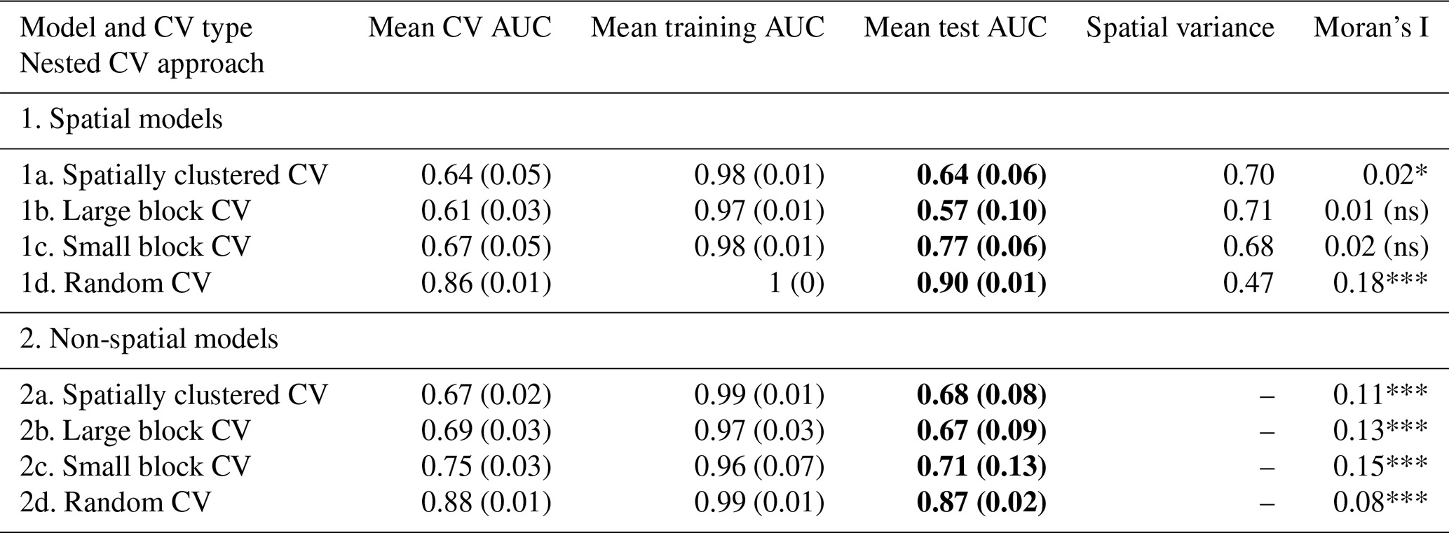
The only models to remove residual spatial autocorrelation were the spatial models parameterised with small or large block CV (models 1b and 1c), although the spatial clustering CV (model 1a) was also close (Table 1) as 4 of 5 of the spatial CV inner loop models successfully accounted for spatial structure (not shown). The model performance metrics further suggest that random CV and non-spatial approaches to ML landslide modelling do not adequately account for spatial structure in the data. Yet, the inclusion of the Gaussian term in the spatial models also has disadvantages as it explains most of the observed variance in landslide occurrence (68 %–71 % in models 1a–1c; Table 1) leaving little to be learned by the predictor variables, and is associated with relatively low predictive performance. Out of the models accounting for spatial structure, the small block CV approach provides the better predictive performance with a test AUC of 0.77 (Table 1). At the other extreme, the random CV method provided highest predictive power, particularly when spatial structure is incorporated into the model (Mean test AUC 0.87 and 0.90 respectively; Table 1).

Table 1 Mean (and standard deviation) model performance metrics of two Gaussian Process Gradient Boosted classification models using four different cross-validation (CV) methods on the full landslide dataset. AUC=area under the curve, where values close to 1 indicate near perfect accuracy of landslide/control point classification. Mean CV AUC=mean value from hyperparameter search (Step 4 in Fig. 3); Mean training AUC=mean value from inner loop training models (Step 5 in Fig. 3); Mean test AUC = mean value from testing inner loop models (Step 6 in Fig. 3) is shown in bold as it is the most useful metric for evaluating performance. Spatial variance indicates the amount of variance explained by the spatial structure of the model (absent from non-spatial models). The significance of the Moran's I test for spatial autocorrelation is indicated by asterisks ($***=p<\mathrm{0.001}$, $**=p<\mathrm{0.01}$, $*=p<\mathrm{0.05}$, ns=non-significant). A significant Moran's I indicates that residual spatial autocorrelation is likely.

The comparison of variable importance across the different model structures (with and without a spatial Gaussian process term) combined with four different cross-validation schemes shows significant variations across the eight tested models on the full dataset (Fig. 4), both in absolute magnitude (mean absolute SHAP values) and in relative ranking. In the spatial models, the effect of the different CV schemes on variable importance is substantial: spatially clustered and large block CV have commonly low variable importance (mean absolute SHAP values<0.05 for all but the top four predictors) and small block CV occupies an intermediate position, while variable importance under random CV is markedly higher than under any other scheme (Fig. 4). Cross-validation scheme had a much smaller effect on variable importance in the non-spatial models (Fig. 4). In all non-spatial models, irrespective of the CV scheme, precipitation intensity (max 3 h precipitation during “Hans”), precipitation (accumulated over 3 d in mm), bedrock weatherability and deposit thickness are consistently amongst the top four predictors (Figs. 4, E4a, E4c, E5a and E5c). For the spatial models, the top four predictors are northerness, flow accumulation, elevation and relative precipitation for the three spatial CV schemes (Figs. 4, E4b, E4d and E5b), while bedrock replaces flow accumulation in the spatial model with random CV (Fig. E5d).

Figure 4 Full factorial comparison of variable importance scores for the full dataset, comparing non-spatial (No spatial GP term) with spatial (Spatial GP term) models built with all four cross-validation (CV) schemes. Variable importance was quantified using mean absolute SHAP (SHapley Additive exPlanations) values.

To explore the underlying causes of these sharp changes in variable importance across model structure and CV schemes, we examined predictor collinearity and residual predictor autocorrelation (Appendix D). First, pairwise predictor correlations show that there is only one strong correlation between surficial deposits and deposit thickness (Cramer's V 0.82; Fig. D2) and one moderate correlation between planar and profile curvature (Spearman's −0.49; Fig. D1). All other correlations are between −0.4 and 0.4 (Figs. D1 and D2).

Second, the variogram analysis (Table D1) provides a CV scheme-specific estimate of how much spatial correlation in each predictor remains at the characteristic distance separating training and test observations. Several predictors, including elevation, groundwater and all three precipitation variables showed effective variogram ranges on the order of tens of kilometres, indicating a high level of spatial structure. Evaluated at the median nearest-neighbour distance under random cross-validation, residual spatial correlation for these predictors approached unity, indicating that a held-out observation's value for these predictors was, on average, almost indistinguishable from that of its nearest training observation under this scheme (Table D1). Residual correlation generally dropped sharply under all three spatial CV schemes, although relative precipitation retained moderate autocorrelation compared to other variables. It is noteworthy that importance under random cross-validation also increased for several predictors with comparatively short spatial ranges (e.g. northerness, flow accumulation, profile and planar curvature; Table D1), a pattern not directly accounted for by predictor-level spatial autocorrelation.

Data exploration of predictor effects using SHAP dependence plots indicated that directional effects of explanatory factors, asymptotic values and the nature of the most important interaction for each variable are relatively consistent across the tested full models (not shown). The SHAP importance plots for the spatially clustered CV in the spatial model (model 1a; Fig. 5a) and non-spatial model (model 2a; Fig. 5b) exemplify the differences in variable importance between the model types described above. The spatial model differentiates more between variables where top four variables have much higher importances than others, while the non-spatial model shows a more even spread across a larger number of variables (Fig. 5a and b). Further, SHAP dependence plots of the four top predictors in model 1a (Fig. 5c–f) indicate some key patterns in the way these variables contribute to landslide occurrence probability. For instance, south-facing slopes are more likely to give rise to shallow landslides than slopes with northern aspects (Fig. 5c). The interaction with relative “Hans” precipitation suggests that south-facing slopes that received high relative precipitation make shallow landslides less likely while north-facing slopes that received highest relative precipitation have increased landslide probability (Fig. 5c). The strong influence of elevation is due to large positive contributions to the probability of landslide occurrence at elevations lower than ca. 480 m a.s.l., while elevation does not contribute to explaining shallow landslide starting points above this elevation (Fig. 5d). Interaction with precipitation intensity further suggests that some of these landslide occurrences at lower elevations may be driven by particularly high 3 h rain intensities. An underlying sampling bias in the landslide point dataset due to availability of post-event orthophotos at lower elevations was considered as explanation but can be rejected as the shallow landslide starting points are normally distributed across the observed elevation range. Flow accumulation values between 0.1and 30 km² contribute positively to landslide probability, in particular on east-facing slopes (Fig. 5e). Relative precipitation does not make clear contributions to the model before reaching double the amount of normal August precipitation when it contributes positively to the probability of shallow landslides on north-facing slopes and negatively on south-facing slopes (Fig. 5f).

For comparison, the top four predictors in the non-spatial model with spatially clustered CV (model 2a; Fig. 5b) are shown in Appendix E. They show that precipitation intensity of 10–16 mm per 3 h (Fig. E1a), total “Hans” precipitation of 100–140 mm (Fig. E1b), fine-grained bedrock including phyllite (Fig. E1c) and surficial deposits greater than 0.5 m (Fig. E1d) all contribute to higher landslide probability.

Figure 5 (a, b) Shapley value summary plots for model 1a (spatial model with spatially clustered CV) and model 2a (non-spatial model with spatially clustered CV. Note the dynamic SHAP value ranges on the x-axes. The numbers after variable names are mean absolute SHAP values, representing relative importance. Points are coloured by normalised feature value. (c–f) Partial dependence plots for the top four variables of model 1a. Each point represents an observation and is plotted with its feature value on the x-axis and SHAP value (contribution to model output) on the y-axis. SHAP values above 0 indicate that a feature value is likely to make a positive contribution to the probability of a landslide. Points are coloured by a second feature chosen to minimise the variance of the SHAP value given both features and represents the strongest interaction. Solid red lines are LOESS smoothed lines and shading represents 95 % confidence intervals.

5.2 Forest models

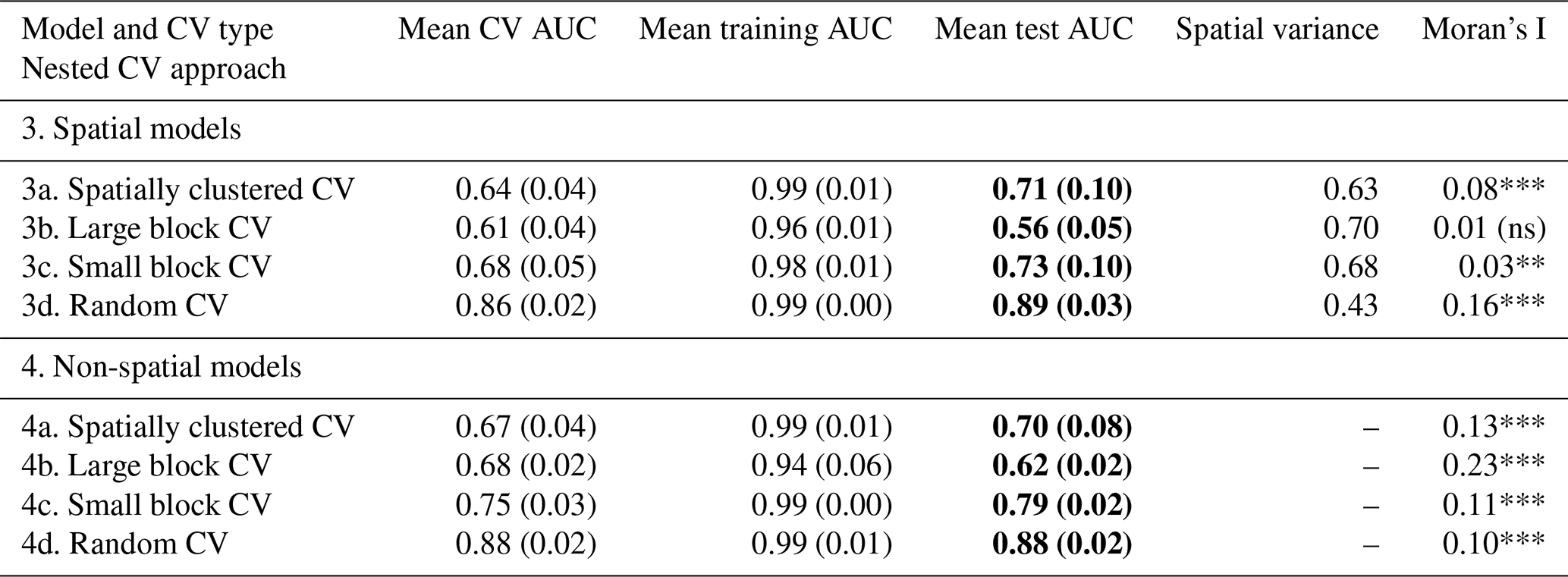
The same modelling runs as presented above for the full dataset were repeated based on the subsampled forest-only dataset consisting of 339 shallow landslide starting points and 434 control points. Similar tendencies in model performance were found as with the full data models, although only the spatial model with large block CV fully accounted for residual spatial autocorrelation. However, the spatial model with small block CV was close (Moran's I 0.03; Table 2) and could have had a lower Moran's I values with some manipulation of the block size and number. For the forest-only dataset, the relatively low number of landslide points makes it difficult to create spatial blocks with balanced and sufficient test landslides, suggesting that a dataset of this size may be on the borderline of successfully applying this approach. Since the test AUC of the large block CV model is barely better than random guessing (0.56; Table 2), we again suggest that this may present the best trade-off between predictive power and over-optimistic performance, even though the small block CV model does not fully account for spatial autocorrelation.

Table 2 Mean (and standard deviation) model performance metrics of two Gaussian Process Gradient Boosted classification models using four different cross-validation (CV) methods on the forest-only landslide dataset. AUC=area under the curve, where values close to 1 indicate near perfect accuracy of landslide/control point classification. Mean CV AUC=mean value from hyperparameter search (Step 4 in Fig. 3); Mean training AUC=mean value from inner loop training models (Step 5 in Fig. 3); Mean test AUC=mean value from testing inner loop models (Step 6 in Fig. 3) is shown in bold as it is the most useful metric for evaluating performance. Spatial variance indicates the amount of variance explained by the spatial structure of the model (absent from non-spatial models). The significance of the Moran's I test for spatial autocorrelation is indicated by asterisks ($***=p<\mathrm{0.001}$, $**=p<\mathrm{0.01}$, $*=p<\mathrm{0.05}$, ns=non-significant). A significant Moran's I indicates that residual spatial autocorrelation is likely.

As in the full model, the importance for each variable under different CV schemes in the forest-only models are more consistent in the non-spatial models than in the spatial models and the observed ranges of mean absolute SHAP values under both model structures are also comparable (Fig. 6). However, the differences between the CV scheme are more pronounced than for the models based on the full dataset, both in the non-spatial models and further amplified in the models with a spatial GP term (Fig. 6). Notably all models with large block CV suffer from low mean absolute SHAP values (<0.04 for most variables), while spatially clustered CV has commonly second highest mean absolute SHAP values behind random CV. We attribute this instability to the smaller sample size for the forest dataset (773 points), which is likely to reduce statistical power, particularly when our CV strategies draw unequal sample sizes across folds.

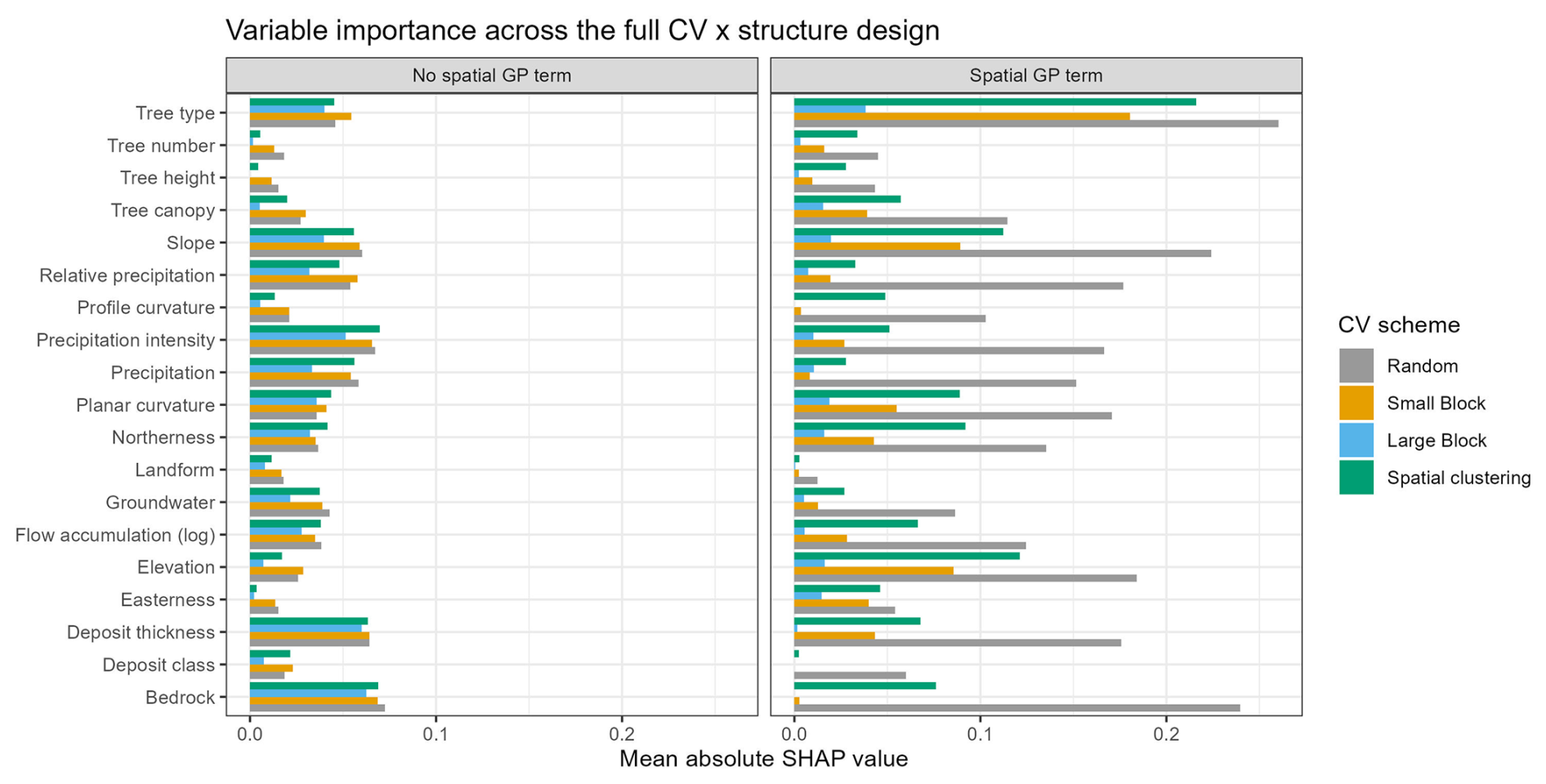
Figure 6 Full factorial comparison of variable importance scores for the forest dataset, comparing non-spatial (No spatial GP term) with spatial (Spatial GP term) models built with all four cross-validation (CV) schemes. Variable importance was quantified using mean absolute SHAP (SHapley Additive exPlanations) values.

In all non-spatial models, the top four predictors are bedrock weatherability, precipitation intensity, deposit thickness and slope (Figs. 6, E5a, E5c, E6a and E6c). For the spatial models the typical top four variables are tree type, slope, elevation and planar curvature (Figs. 6, E6d and E7b), while northerness and bedrock weatherability replace planar curvature in the top four under spatially clustered CV (Fig. E6b) and random CV (Fig. E7d), respectively. The strongest forest-specific variable correlations are found between tree canopy and tree number, tree canopy and tree height (Spearman's 0.70 and 0.50; Fig. D3), and tree type and tree height (Cramer's V 0.51; Fig. D4). Variable autocorrelation results for the forest-only models are similar to those for the full model (Table D2). Amplified variable importance under the random CV scheme, in particular when combined with a spatial random effect, concerns variables with strong spatial structure (elevation, bedrock and all three precipitation variables) as well as those with finer-scale structure (e.g. tree type, slope and planar curvature).

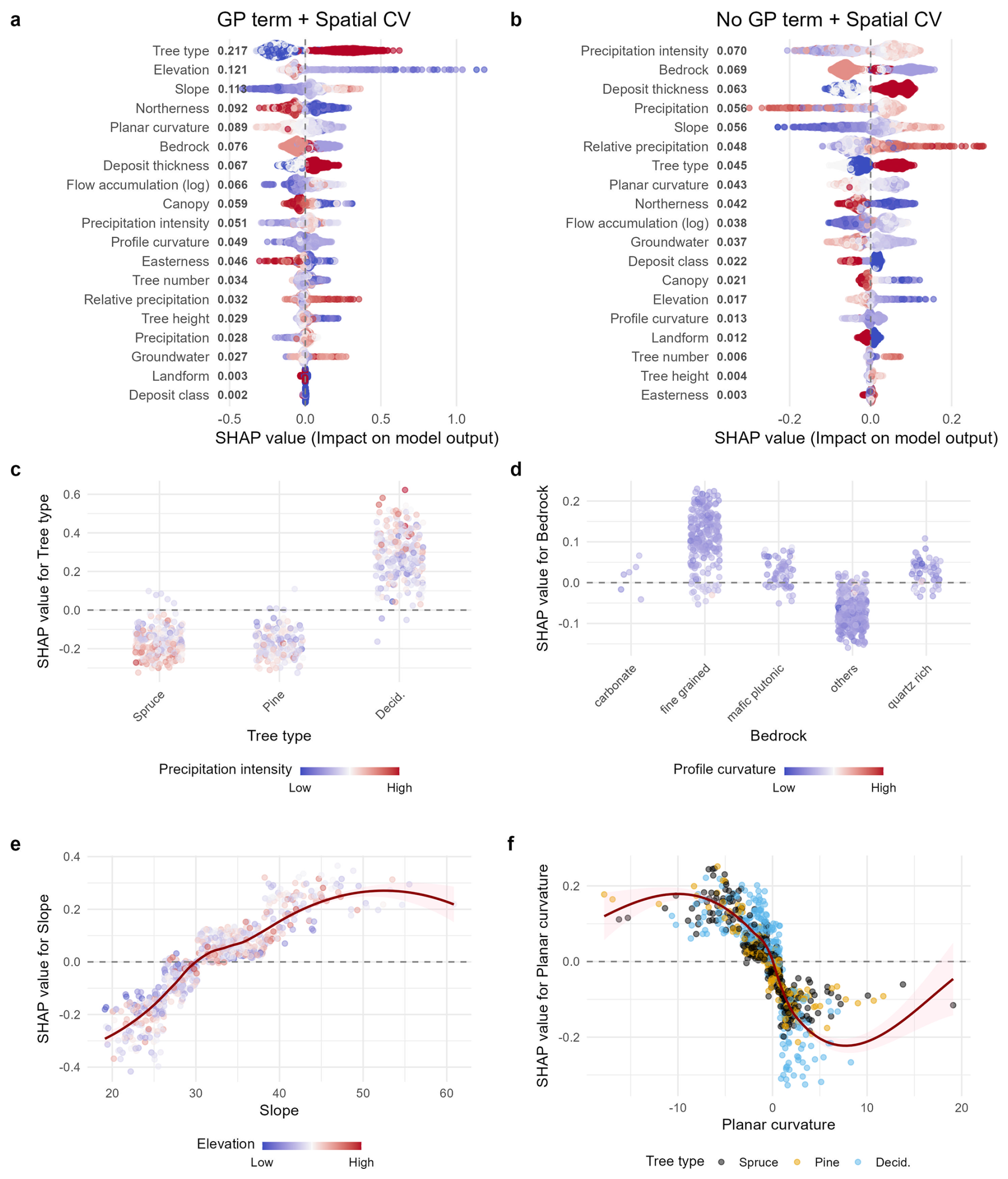
Figure 7 (a, b) Shapley value summary plots for forest-only model 3a (spatial model with spatially clustered CV) and model 4a (non-spatial model with spatially clustered CV). Note the dynamic SHAP value ranges on the x-axes. The numbers after variable names are mean absolute SHAP values, representing relative importance. Points are coloured by normalised feature value. (c–f) Partial dependence plots for four important variables of model 3a. Each point represents an observation and is plotted with its feature value on the x-axis and SHAP value (contribution to model output) on the y-axis. SHAP values above 0 indicate that a feature value is likely to make a positive contribution to the probability of a landslide. Points are coloured by a second feature chosen to minimise the variance of the SHAP value given both features and represents the strongest interaction. Solid red lines are LOESS smoothed lines and shading represents 95 % confidence intervals.

To provide an example of the forest-only model results, we again explore the spatial and non-spatial models with spatially clustered CV in greater detail (Fig. 7). Elevation and northerness are amongst the top four variables of the spatial model with spatially clustered CV (model 3a). Since their effects are similar to those based on the full dataset (model 1a) with increased landslide probability at elevations below 480 m a.s.l. (Fig. 5d) and on south-facing slopes (Fig. 5c), we rather show planar curvature and bedrock ranking 5th and 6th in model 3a in the SHAP dependence plots (Fig. 7c–f). The modelled effect for tree type suggests that forested areas dominated by spruce and pine stands make landslide occurrence less likely, particularly in areas with the highest precipitation intensity (Fig. 7c). By contrast, deciduous forest stands contribute positively to landslide probability, again especially under the highest rainfall intensities (Fig. 7c). Landslide occurrences in forest are also most likely for bedrock weatherability class 2, dominated by phyllite (Fig. 7d). While shallow landslides released during the “Hans” storm included relatively low slope angles outside of the forest, slope angles above a threshold of 30° increase the likeliness of landslide occurrence in the forest (Fig. 7e). Slope angles below 30° reduce the likeliness of landslides, in particular at low elevations. Negative planar curvature values, corresponding to channelised terrain, increase landslide probability, an effect which is most pronounced in deciduous forests (Fig. 7f).

The top four predictors of the non-spatial model with spatially clustered CV are identical based on the full (model 2a; Fig. 5b) and forest-only datasets (model 4a; Fig. 7b). Model 4a thus shows that precipitation intensity of 10–16 mm per 3 h (Fig. E2a), fine-grained bedrock including phyllite (Fig. E2b), surficial deposits greater than 0.5 m (Fig. E2c) and total “Hans” precipitation of 100–140 mm (Fig. E2d) all contribute to higher landslide probability in the forest. Notably, apart from tree type, the only other forest parameter to explain shallow landslide starting points reasonably well is canopy cover, while tree number and tree height (moderately correlated with tree type and canopy cover) have relatively low mean SHAP values in all forest models. Nevertheless, SHAP dependency plots for all forest variables in model 3a suggest that spruce and pine forests (Fig. E3a), with 750–1750 trees per ha (Fig. E3b), tree heights of 100–175 m (Fig. E3c) and canopy cover above 75 % (Fig. E3d), reduce the likeliness for landslide release on forested slopes.

6 Discussion

In the following, we will discuss our objectives. To start with, we advocate for our approach in beginning to address the problem of overfitting in landslide modelling with machine learning methods, acknowledging the potential tension between quantitative performance metrics and geomorphologic plausibility (first objective O1; Sect. 6.1). Then, we discuss the impact of consistently important variables in the full models (second objective O2; Sect. 6.2). Further, we demonstrate the important role of forest characteristics in influencing landslide susceptibility based on the forest-only models (third objective O3; Sect. 6.3), before providing a synthesis and outlook (Sect. 6.4).

6.1 Quantitative model evaluation versus plausibility

Both landslide and control points exhibited strong spatial autocorrelation as raw data (test not shown) and as model residuals, at least for those models that did not adequately address the issue. As a result, models that failed to account or only partially accounted for spatial autocorrelation had highest evaluation metrics (test AUC of more than 0.88), comparable to recent studies of landslide modelling with gradient boosting (Choubin et al., 2025; Dai and Huang, 2025; Liu et al., 2021; Cao et al., 2020). However, we argue that such models should be viewed with caution because the results may be biased, over-optimistic and may identify important predictor variables that primarily capture spatial covariance rather than mechanistic relationships (Roberts et al., 2017; Urdangarin et al., 2023). As has been argued elsewhere, finding the right balance between quantitative performance evaluation and interpretability or geomorphic plausibility in shallow landslide susceptibility mapping can be challenging (Steger et al., 2016, 2021; Schlögl et al., 2025; Lima et al., 2021). We discuss the observed large differences in variable importance in the spatial models versus non-spatial models and between models with random versus spatial cross-validation in this context.

In the full and forest-only dataset, models with and without the Gaussian spatial term identified completely different top predictors. These switches in variable importance can be due to a number of statistical artefacts. High collinearity can cause conflicting variable importance (Schlögl et al., 2025; Steger et al., 2024, 2021). In our study, pairwise associations for all predictor variables (Figs. D1–D4) show mostly moderate collinearity among a few directly related variables (planar vs. profile curvature and three pairs of forest variables). The exception is a strong association between surficial deposits and deposit thickness (Cramer's V=0.82), which likely reflects their direct conceptual relationship rather than independent spatial proxying. This suggests that raw predictor collinearity is unlikely to fully explain the observed differences in variable importance across modelling approaches.

Another issue can be cross-validation data leakage, where train-test splits are too close together for highly structured predictors, compromising the independence of evaluation data and producing overly optimistic performance metrics (Roberts et al., 2017). Our analysis suggests that this was largely accounted for in the most conservative spatial cross-validation schemes, although it often came at the expense of predictive performance. Under random cross-validation, for the variable with strongest spatial structure – relative precipitation – test and nearest training points have on average indistinguishable variable values. While the residual correlation dropped sharply under all three spatial cross-validation schemes, relative precipitation still retained moderate autocorrelation and should be viewed with caution.

A third explanation is that the spatial models suffered from spatial confounding, where predictors are correlated with spatial random effects (Urdangarin et al., 2023). When including a spatial term, key predictors in the non-spatial models with strong spatial structure (total precipitation, precipitation intensity) and with medium-range structure (bedrock weatherability, deposit thickness) lose much of their apparent importance under all cross-validation schemes except random CV. This may suggest they act as proxies for spatial structure in the non-spatial models, capturing spatial patterns in landslide occurrence in the absence of explicitly modelled structure. If this is the case, their importance is likely inflated in non-spatial models and/or suppressed in spatial models, where the Gaussian spatial term seems to capture the same variability more effectively than the covariates themselves. The latter is likely considering relatively coarse and possibly biased datasets including the meteorological products at 1 km spatial resolution with sparse direct observations in mountainous areas (total precipitation, precipitation intensity) and categorical maps with highly variable spatial detail (deposit thickness, bedrock weatherability).

Taken together, our diagnostics and results indicate that no single combination of cross-validation scheme and model structure simultaneously achieved strong predictive performance, non-significant residual autocorrelation together with importance estimates free from collinearity, leakage or confounding effects. We therefore do not identify an optimal model configuration among those tested and suggest that future modelling studies explore methods to isolate spatial structure from raw data before modelling, such as via the Spatial+ statistical framework (Dupont et al., 2022). Nonetheless, the presence of groups of consistently important (and consistently unimportant) variables together with dependence plots, consistent across models in terms of shape and direction, gives us sufficient basis to attempt an interpretation of the observed patterns.

Figure 8 (a) Maximum 3 h precipitation summed up for the “Hans” time period based on the MET Nordic dataset, shallow landslide starting points symbolised with colours corresponding to rainfall intensity and control points in transparent grey for reference (b) Bedrock weatherability classes and shallow landslide starting points symbolised with colours corresponding to weatherability classes. © Kartverket, SeNorge, NGU.

Because the role of total “Hans” precipitation, precipitation intensity and bedrock weatherability is difficult to discern, we explore plausibility in terms of their spatial distribution and potential combined effects. Our control point sampling approach (Sect. 3.2) reduces the influence of relative precipitation to effects within observed attribute ranges. Nevertheless, it is the most important meteorological variable in the spatial full models under the spatial CV schemes (Fig. 4b) and in spatial forest model with random CV (Fig. 6b). Based on simple visual examination, it seems plausible that relative precipitation (“Hans” precipitation relative to normal August precipitation; Fig. 1b) has greater explanatory power than precipitation magnitude (total “Hans” precipitation; Fig. 1a) because several parts of western Norway received “Hans” precipitation with comparable magnitude as the heaviest affected areas in the east without consequences like flooding and shallow landslide occurrence. The lack of consequences in western Norway is likely related to smaller and steeper catchment areas and soil that are better adapted to receiving high amounts of rainfall in western Norway (Ekholt, 2023). The spatial distribution of precipitation intensity during the “Hans” storm (Fig. 8a), suggests that shallow landslides did not occur in the areas with highest rainfall intensities which is in line with modelling results suggesting highest landslide susceptibility for 10–16 mm precipitation per 3 h (Figs. E1a and E2a). Areas in the southeast with “Hans” rainfall intensities in this range have steep enough slopes to give rise to landslides as illustrated by the placement of numerous control points (Fig. 8a).

Bedrock weatherability (Fig. 8b) can potentially explain why very few shallow landslides were triggered in these southeastern areas as well as in western Norway despite favourable meteorological conditions (precipitation magnitude and intensity). Since the national bedrock map differentiates the main bedrock type into 121 categories (NGU, 2025a), the dataset was reclassified into five weatherability classes based on the anticipated effect of physical and chemical weathering in a polar climate (Hakim et al., 2021; Momeni et al., 2015). To our knowledge, this is the first time this has been done in the context of landslide susceptibility mapping. Weatherability class 2 (shales, phyllites) contributes most positively to landslide probability, while the contribution of classes 1 (carbonous rocks), 3 (mafic plutonic rocks) and 5 (quartz-rich rocks) is indecisive and class 4 (sandstones, conglomerates, felsic volcanic and metamorphic rocks) reduces chances of landslide occurrence (Figs. 7d, E1c and E2b). There is a striking co-occurrence of weatherability class 4 (Fig. 8b) with areas which experienced 10–16 mm of 3 h rainfall in eastern Norway and areas with 100–140 mm of 3 d rainfall in western Norway without triggering any landslides (Fig. 8a). This suggests both (1) that soil in these areas with slowly weathering bedrock might be generally thinner and less stratified (Cámara et al., 2017), and thus less susceptible to shallow landslides; and (2) that the combination of top predictors precipitation, precipitation intensity and bedrock weatherability observed in the non-spatial models is geologically plausible.

6.2 Hydrometeorological conditions and soil indicators explain landslide susceptibility partly

Rainfall-induced shallow landslides release when a critical porewater pressure in the soil is reached, i.e. rainfall intensity and surface runoff in combination exceed the hydraulic drainage capacity of the subsurface (Bogaard and Greco, 2016; Guzzetti et al., 2008). Therefore, water supply is key to determining susceptibility to shallow landslides for a given event. While precipitation amount and intensity as well as precedent groundwater level are event-specific, flow accumulation is a DEM derivative and a constant measure of the upstream drainage areas into each grid cell giving good indications of the amount of expected surface runoff whilst neglecting the effect of water infiltration. Flow accumulation is therefore one of three topographic variables considered in the national shallow landslide susceptibility map (Fischer et al., 2012; Pullarello et al., 2025). Norway's land surface is categorised into three susceptibility zones depending on shallow landslide activity levels and applied threshold values for flow accumulation vary from 3500–9000 m² within susceptibility zones. Our results suggest that flow accumulation greater than 100 000 m² contributed to increased landslide release probability during the “Hans” storm (Fig. 5e). This is a relatively high flow accumulation value that would normally correspond to permanent streams (Rüther et al., 2022), and it may indicate an inventory bias towards debris floods that were supposedly excluded from the dataset (Sects. 2 and 3.1). But it could also be the result of considering the maximum flow accumulation for a 30 m buffer surrounding landslide and control points (Sect. 3.3).

Another factor which is known to contribute to shallow landslide release are pre-event groundwater conditions as saturated soils prior to rainstorms increase chances of shallow landslide triggering (Bondevik and Sorteberg, 2021; Johnson and Sitar, 1990; Montgomery et al., 2009). In most of the tested models, pre-“Hans” groundwater level relative to normal for the same day (modelled for 7 August 2023, 8 a.m.) only increased landslide probability where it exceeded 170 % (not shown), a relative value which is only attained at low elevations (Fig. 9a). As such, these high values may not be representative of the shallow landslide release areas, but rather an effect of the coarse nature of the modelled groundwater data (1 km resolution). Relative groundwater levels between 125 % and 170 % even reduce landslide probability, which is probably due to its spatially extensive occurrence in eastern Norway (Fig. 9a), making it an imprecise indicator.

Figure 9 (a) Modelled pre-“Hans” groundwater level compared to normal (1981–2010) for 7 August 2023, 8 a.m. and shallow landslide starting points symbolised with colours corresponding to groundwater level. (b) Shallow landslide starting points in the study area with those under 480 m a.s.l. highlighted in lighter brown. © SeNorge, Kartverket.

Despite the chosen control point sampling method, elevation is amongst the top predictors in all full spatial models and has moderately high importance in the non-spatial models (Fig. 4). Elevation does not have significant collinearity with other included variables (Figs. D1 and D3) and its importance is driven by the positive contribution of elevation under 480 m a.s.l., interacting most strongly with precipitation intensity (Fig. 5d). Elevation indirectly impacts landslide occurrence due to variations in environmental variables like temperature, rainfall regime and vegetation (Catani et al., 2013; Quevedo et al., 2022) and may thus be a placeholder for explanatory factors that are either not included or represented by imperfect datasets. Numerous debris slides and small debris flows were released in low-lying agricultural hillslopes of Hallingdal, Valdres and Gudbrandsdalen (Figs. 9b and 10). The categorical variable “landuse” has been excluded from the machine learning models due to a large imbalance as only seven control points fell in the category of agricultural land. Thus, the strong influence of elevation may suggest that it operates as a proxy for agricultural land. However, the higher probability of landslide occurrence at low elevation is not restricted to agricultural land alone because elevation was also important in the forest-only spatial models.

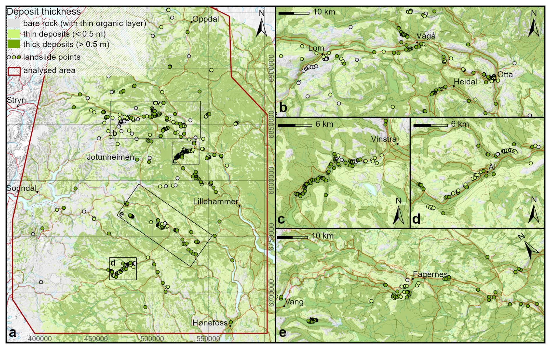
Figure 10 Spatial distribution of the categorical variable deposit thickness and shallow landslide starting points symbolised with corresponding colours for (a) the entire study area, (b) Ottadalen, (c) Skåbudalen, (d) inner Hallingdal and (e) Valdres. © Kartverket, NGU.

Impressions from fieldwork in the valleys of Hallingdal, Valdres and Gudbrandsdalen (Figs. 9b and 10) further suggest that the majority of shallow landslides were released in connection with excessive surface runoff, often redirected along forest roads and sometimes in anthropogenically influenced surficial deposits. Ideally, a variable considering distance to forest roads should have been included in the model, but there is no complete and updated dataset over Norwegian forest roads. It is also possible that elevation functions as a proxy representing anthropogenic terrain interventions as they are likely to be more extensive with decreasing elevation. In addition, the effect of elevation under 480 m a.s.l. may correspond to areas with particularly thick and stratified soils. Numerous studies suggest increased shallow landslide susceptibility with soil thickness (e.g. Thiery et al., 2014; Cascini et al., 2017; Guzzetti et al., 1999). Thin soils have been shown to correlate with greater scree cover and exhibit higher infiltration capacity and lower erodibility (Fu et al., 2011). Moreover, soil depth as well as soil characteristics including stratification have been shown to be crucial in modelling shallow landslide occurrences (Kim et al., 2015; Tofani et al., 2017). Thicker soils are thus more likely to be heterogeneous. Heterogeneity in the subsurface includes impermeable soil layers and spatial variability of layer thicknesses which both contribute to the build-up of locally elevated porewater pressures and triggering of shallow landslides (Johnson and Sitar, 1990; Tufano et al., 2021; Oguz et al., 2022). We therefore suggest that the effect of elevation interacting with precipitation intensity (Fig. 5d) is a mixture of anthropogenic influence and thicker, more stratified soils at elevations below 480 m a.s.l. that received high 3 h precipitation during the “Hans”-storm.

Deposit thickness is amongst the top predictors in all full and forest-only non-spatial models, while its importance in the spatial models is limited to those with small block and random CV (Figs. 4 and 6). As it is a categorical variable with only three classes, it likely does not reflect variations in soil thickness, let alone soil characteristics, in great enough detail (Fig. 10). As summarised in the above paragraph, the influence of deposit thickness on landslide probability is well documented. Yet, data availability is often limited, and most studies rely on soil thickness modelling approaches (Dietrich et al., 1995; Moore et al., 1993; D'Odorico, 2000), more recently supported by machine learning (Baltensweiler et al., 2021; Gomes et al., 2023; Wadoux et al., 2020). The deposit thickness dataset included in this study is a biproduct of the national surficial deposit map and based on direct observations but at highly variable spatial scale (NGU, 2025c; Fig. 10).

Northerness is amongst the top variables in the full and forest-only spatial models, but it has also moderate to high importance in the non-spatial models (Figs. 4 and 6). Aspect is commonly considered in studies of landslide susceptibility, mostly as it influences evapotranspiration and weathering processes and consequently vegetation and root development (Sidle and Ochiai, 2006). As the “Hans” low-pressure system approached Norway from the southeast, one may also expect more precipitation on the windward mountain slopes, with southern and eastern aspects. This orographic effect may not be adequately reflected in the available gridded precipitation data with 1 km resolution. While southern aspects clearly increased the probability of shallow landslides during the “Hans”-storm, the variable easterness is less influential with low importances in most models. Moreover, the models suggest west-facing slopes were slightly more susceptible to shallow landslide occurrence during “Hans” than east-facing slopes, making an orographic effect less likely. Whilst the observed effects of aspect on landslide probability may be related to differences in vegetation, northerness explains landslides less well in the forest models than in the full models and, therefore, we argue that aspect could also be understood as a proxy for soil thickness and characteristics. Due to reduced weathering rates soils at comparable elevations will likely be thinner and less stratified in northern and eastern aspects compared to south- and west-facing slopes. While this directional effect is well-known for mechanical weathering in Norway due to fewer freeze–thaw cycles on north- and east-facing slopes, it may also include biological weathering, as smaller species diversities on north-facing slopes (Heikkinen, 1991; Parker, 1988) may reduce organic and regolith production (Phillips et al., 2021; Sidle and Bogaard, 2016). The suggested interaction of northerness with relative precipitation (Fig. 5c) is interesting in this context, as it suggests that north-facing slopes are most prone to the occurrence of shallow landslide when exposed to close to double the amount of normal August precipitation. South-facing slopes on the other hand, increase landslide probability in general while reducing it in areas with high relative precipitation (Fig. 5c). In relatively thick and stratified soil cover on southern and western slopes, the chances of building up sufficient pore pressure over an impermeable soil or bedrock layer are higher than over a thinner, more homogeneous soil cover which often have higher infiltration capacity (e.g. Tufano et al., 2021) on northern and eastern slopes. Observations from the Jølster event on 30 July 2019 in western Norway indicate that thin soil may be more susceptible to shallow landslide releases than thicker soil given extraordinary rainfall intensities (Rüther et al., 2022).

6.3 Forest effects on shallow landslide susceptibility

Vegetation, and most importantly trees, are drivers of slope stability through mechanical effects (Waldron, 1977; Wu et al., 1979) and hydrological effects, including interception of precipitation, root water uptake and evapotranspiration (Kim et al., 2017). Amongst the mechanical effects root networks, in particular fine roots with diameters smaller than 2 mm, provide tensile strength to the soil (Schwarz et al., 2010b), while the surcharge of trees as well as drag forces due to wind may influence slope stability slightly negatively (Fan and Lai, 2014; Kim et al., 2020). Due to the combined hydrological and mechanical reinforcement effects provided by vegetation and forests, they are a part of what is coined Nature-based Solutions (NbS; Capobianco et al., 2025; De Jesús Arce-Mojica et al., 2019), meaning that when managed correctly, forests may reduce shallow landslide risk.

Figure 11 (a) Tree type and shallow landslide starting points symbolised according to tree type. (b) Canopy cover and shallow landslide starting points symbolised according to canopy cover. © Kartverket, NIBIO.

In our models, trees were indeed found to be important to landslide probability, but only tree type was a consistent influential forest variable across both spatial and non-spatial forest-only models, with highest shallow landslide probability in deciduous stands (Fig. 7c). Tree type is known to influence slope stability due to differences in root systems, which determine how much tensile strength trees provide within the soil, across potential soil boundaries and potentially across the soil-bedrock-interface. Both spruce and birch, the most common deciduous tree in Norway, have relatively shallow root systems, while pine has a more substantial root system and anchors the soil to the bedrock substrate (Kutschera and Lichtenegger, 2002). However, the growth of the important fine root system has also been shown to depend on nutrient availability in the soil and competition from other species (Schmid, 2002). Planted spruce on steep slopes is seen as a particular threat to slope stability after clear-cutting or due to uprooting of older stands (Sidle, 1992). Therefore, the fact that deciduous forest shows the greatest susceptibility to shallow landslide occurrence, while spruce and pine forests reduce landslide susceptibility, may seem surprising at first as their provided mechanical reinforcement is not expected to be any lower than in spruce forest. While the hydrological effect of root water uptake cannot easily be estimated from aggregated forest data as root water uptake has been shown to depend on both under- and overground species interactions (Kinzinger et al., 2023), canopy cover may provide an estimate to the effect of interception. Amongst landslide starting points in deciduous forest, mean canopy cover (70.4 %) is comparable to spruce forest canopy (70.5 %), while pine canopy is less dense on average (61.9 %). Thus, the hydrological effect of interception probably does not explain the observed higher landslide susceptibility in deciduous forest either. It is more likely that greater susceptibility of deciduous forest to shallow landslides under “Hans” is an indication of the type of terrain and soils where this forest typically grows, i.e. in steep terrain not suited for production forests and in relatively thin soils towards the tree line (Fig. 11a).

Tree canopy cover (Fig. 11b) is the only other forest variable with at least moderate importance in most models (Fig. 6), and suggests that forests in general and deciduous forest in particular, contribute to stability when canopy cover exceeds 75 % (Fig. E3d). Tree number and tree height have low importance values in all forest-models (Fig. 6). This may suggest that the forest inventory SR16 at 16 m resolution (Astrup et al., 2019; Breidenbach et al., 2021; Hauglin et al., 2021) is too coarse to adequately represent forest structure but could also result from these variables' moderate collinearity with canopy cover and tree type. In general, the forest-only dataset was probably too small for our analysis methods, highlighting a key weakness of event-based susceptibility studies: when sample sizes are small, variables are poorly represented, model uncertainty is higher and predictors more likely to be insignificant (Smith et al., 2023). We recommend that future landslide susceptibility studies explore the importance of trees further, incorporating larger, multi-temporal inventories and more detailed forest structure datasets.

Across both spatial and non-spatial models with different CV sampling methods, slope angle appeared to be more important in the forest-only models compared to their full model counterparts. It is important to note that the sampling of control points within observed landslide slope ranges likely reduced the significance of slope in the full models. Typically, slope is the most powerful morphological variable and particularly effective in explaining the spatial distribution of landslides (Reichenbach et al., 2018; Corominas et al., 2014; Malamud et al., 2004). Slope ranges for the “Hans”-induced landslide starting points are surprisingly wide ranging from 19–61°. This includes gentler and steeper terrain than typically considered; e.g. the Norwegian shallow landslide susceptibility map considers slope angles of 22–45° for the zones with highest historic activity levels (Pullarello et al., 2025). The mapping approach of the event inventory (Rüther et al., 2024) implies that shallow landslides in the most remote areas are only detected based on satellite data where mass movement processes cannot be determined unequivocally. The inventory may therefore include debris floods that can start in steeper terrain and have longer runouts than debris flows (Church and Jakob, 2020; Hungr et al., 2014) and, in some cases, starting points could have been mapped falsely where debris spreads out from a stream channel at lower slope angles. Despite these mapping-related constraints, “Hans” starting points that were studied in greater detail also suggest an unusual wide range of slope angles. The mean slope angle for landslide starting points in the forest is 33.8° as compared to 28.1° for landslide starting points in agricultural and other open land (the mean slope for all landslide starting points is 31.8°). These observations are in line with the pioneering Swiss study suggesting fewer landslides and higher mean slope angles on forested slopes compared to open land (Rickli and Graf, 2009). 65 % of starting points occurred in the forest, while only 50 % of the mask used for control point selection (Fig. 2) is forest-covered, suggesting a slight overrepresentation of landslide starting points in the forest. However, the ML results clearly suggest that slope angles below 30° contribute negatively to landslide susceptibility, while slope angles above 30 and up to 50° increase landslide probability in the forest (Fig. 7e). This key difference to the full models shows that trees efficiently hinder initiation of shallow landslides in gentler terrain.

Aspect (northerness and easterness), by contrast, appears less important in the forest than in the full non-spatial models, while its importance varies more strongly across the different CV schemes in the forest spatial models (Figs. 4 and 6). As argued above, south- and to a smaller degree west-facing slopes may be more susceptible to shallow landslide initiation due to more active weathering processes and thicker, more stratified soils. It seems that the existence of tree cover makes south-facing slopes slightly less susceptible to landslide release compared to non-forested slopes. The study area is located in the southern polar region where temperature is often the limiting factor for growth in the forest ecosystem and where the highest species diversities have been found on south-facing slopes (Heikkinen, 1991; Parker, 1988). Therefore, forests with higher species diversity may counteract the weathering effects on soil thickness and characteristics by providing mechanical and hydrological reinforcement. Future analyses of non-event specific inventories are recommended to strengthen the argument that higher thresholds for slope and a less pronounced weathering-related effect of aspect can generally be expected in forests in polar climates. If so, the existence of forest and selected forest-specific variables (e.g. tree type, canopy cover) and threshold values (e.g. slope) could become an integral part of an updated Norwegian shallow landslide susceptibility map, potentially transitioning from a knowledge-based (Fischer et al., 2012; Pullarello et al., 2025) to data-driven shallow landslide susceptibility assessment. On a general note, this study demonstrates that forests can reduce shallow landslide risk, highlighting the need for an integral forest management as part of nature-based solutions for mitigation.

6.4 Synthesis and outlook

Despite the strongly shifting ranking of explanatory factors, we found that some of the most consistent variables are comparable to results of the majority of data-driven susceptibility assessments (Lima et al., 2022). However, huge differences in availability, resolution and potential biases of the included datasets as well as the employed statistical or ML analysis methods make a direct comparison extremely difficult. Moreover, model performances have been shown to vary greatly depending on landslide point sampling strategies, ranging from distributed over centroid points for either the entire landslide path or the release area, to points at landslide vicinity (Alvioli et al., 2016; Bordoni et al., 2020; Hong et al., 2019). In contrast, the sampling of non-landslide points does not commonly receive much attention but has been shown to have significant influence on model outcome as well (Dou et al., 2020; Hong et al., 2019). Our control points are sampled within the observed attribute ranges of slope, elevation and relative precipitation in the landslide point inventory. While we expect reduced importance for these variables, both elevation and relative precipitation are consistently important explanatory factors; the latter is underscoring the significance of incorporating rainfall relative to the local climate, in particular when the rainfall event affects large regions. The influence of slope is moderately low in our full models, which is a clear contrast to slope angle being amongst the top predictors in 88 % of recent publications on data-driven susceptibility maps (Lima et al., 2022). Nevertheless, slope plays a more decisive role in the forest-only models illustrating the importance of including forest variables in data-driven shallow landslide susceptibility modelling (Moos et al., 2016) and, more broadly, underscoring the potential in managing forest to mitigate shallow landslides risk (Teich et al., 2022). Aspect and rock type are commonly considered in data-driven landslide susceptibility studies and amongst the top 15 predictors in 73 % of recent studies, while elevation is only used and found to be important by 47 % of recent studies (Lima et al., 2022). While the significance of bedrock can clearly be attributed to differences in weatherability and regolith production rates (Hakim et al., 2021; Momeni et al., 2015), the significance of elevation and aspect is more open to interpretation. In different contexts, they may be proxies for a range of variables which influence slope stability, including distribution of temperature, precipitation, weathering and vegetation (Bordoni et al., 2020; Fabbri et al., 2003; Catani et al., 2013; Quevedo et al., 2022; Sidle and Ochiai, 2006). In this study, elevation, aspect and bedrock weatherability are suggested to be indicative of soil characteristics that are not sufficiently represented in the existing categorical dataset of deposit thickness. Soil thickness and heterogeneity exert a key control on shallow landslide initiation (Bogaard and Greco, 2016; Sidle and Bogaard, 2016), but are generally difficult to access and map.

Furthermore, we have shown that gradient boosted models have potential for understanding and modelling landslide probability but are also highly sensitive to cross-validation techniques and spatial modelling choices. Based on our findings, we suggest that testing of autocorrelation of input data, predictors and model residuals should become an integral part of landslide susceptibility modelling approaches. The spatial autocorrelation in landslide inventories most likely reflects incorrect, incomplete and missing datasets for explanatory factors. However, even given perfect representation of known drivers of slope instability, it is likely that there will remain a spatial component in the data that needs to be accounted for. While we did not find a satisfactory solution to this problem, we have highlighted some important issues that are often overlooked in landslide probability modelling and provide some initial steps in improving model design. Interestingly, it was not sufficient to only model the spatial structure with random effects to address the spatial autocorrelation issue, but hyperparameter tuning also required the spatial structure to be accounted for through spatial clustering of the folds for cross-validation. This process is gaining traction in shallow landslide susceptibility mapping, particularly with the use of Generalised Additive Modelling (Brenning, 2005; Goetz et al., 2015b; Knevels et al., 2023; Steger et al., 2016, 2021) and Random Forests (Schlögl et al., 2025). To our knowledge, fewer studies have modelled the spatial structure directly (Knevels et al., 2023; Steger et al., 2021).

While the novelty in our study lies in addressing the popularity of extreme gradient boosting ML methods and suggesting a similarly robust approach in this space, this analysis is based on a relatively small, event-based inventory with associated advantages and limitations (Oliveira et al., 2024). Therefore, future studies should consider exploring, adapting and testing this methodological approach further afield based on larger, multi-temporal inventories and with the aim to develop a more reliable machine learning protocol for landslide susceptibility. We recommend that future landslide susceptibility studies employing ML methods: (1) test for initial and residual spatial autocorrelation in both response and predictor data, (2) include or explore explicitly modelled spatial structure options, (3) explore and employ several spatial cross-validation techniques for both hyperparameter optimisation and model evaluation, and (4) report complete methodological details to enable reproducibility and proper interpretation of results. Failure to account for spatial structure through appropriate analysis protocols may lead to over-optimistic model performance and misleading interpretations of predictor importance rankings due to spatial confounding. These findings do not invalidate previous endeavours but highlight that performance evaluation and predictor importance from ML studies should be interpreted cautiously if spatial structure has not been explicitly addressed in method descriptions, particularly regarding model generalisability to new spatial locations or future landslide probabilities.

7 Conclusions

In this study, we explore which explanatory factors best explain shallow landslides triggered by the “Hans” storm of 7–10 August 2023. Using 571 mapped shallow landslide starting points from the refined event inventory (Rüther et al., 2024) and 571 control points sampled in the attribute space for slope, elevation and relative precipitation (reduced to 570 landslide and 568 control points due to missing data), we compiled a dataset with 20 explanatory variables. On this basis, we implemented a systematic comparison of 32 gradient boosted decision tree model runs to assess the impact of: (1) the hyperparameter optimisation approach (nested vs. simple cross-validation), (2) spatial structure incorporation (spatial vs. non-spatial models), (3) cross-validation strategy (spatial clustering, large block, small block and random) and (4) applied on the full vs. forest-only dataset. We find that predictive model performance and the degree to which spatial autocorrelation in landslide data is accounted for are often inversely related. Spatial models including a Gaussian spatial term must be combined with spatial cross-validation to effectively control for spatial autocorrelation, although this in turn may lead to spatial confounding issues and methods to isolate spatial structure from true signal should be explored. Models with random cross-validation provided highest performance metrics, but these are likely to be over-optimistic, in particular when a spatial random effect is incorporated into the model. Future studies should further explore this effect to mitigate global overfitting of the spatial gradient boosted model. Based on analyses of the results across the tested model structures and cross-validation schemes, we conclude with the following:

• The top predictors in spatial models differ markedly from those in the non-spatial models. Variable collinearity and strong spatial structure were considered, but spatial confounding is favoured as explanation of alternative key variables.

• The consistent importance of elevation and aspect across models shows that the current seamlessly available soil thickness dataset does not resolve soil thickness, let alone soil heterogeneity sufficiently. Rather, elevations under 480 m a.s.l. as well as south-facing slopes increase landslide probability and are probably related to anthropogenic influences at low elevations, increased weathering rates and thicker and/or more heterogeneous soils.

• The contributions of the various hydrometeorological factors are in line with expectations, showing that the combined effect of water received from precipitation and runoff determines whether critical pore pressure for shallow landslide release are exceeded.

• The classification of bedrock into five bedrock weatherability classes is a useful approach and resulted in high importances in several of the models as class 2 dominated by phyllite increases landslide probability while class 4 dominated by gneisses and granites made landslide release less likely.

• Shallow landslide release in forested areas requires higher slope angles compared to all landslide starting points in the full models suggesting that forested area should be treated differently from non-forested areas in the national landslide susceptibility map. These results also demonstrate the forest's capability as nature-based solution in mitigating against shallow landslide release.

• In tree-covered areas, shallow landslide susceptibility is highest in deciduous forest, which is probably related to the occurrence of birch-dominated forest with relatively low canopy cover towards the tree line and on slopes that are not suited as production forest. Finally, the effect of aspect with increased landslide probabilities on south-facing slopes is less pronounced on forested slopes suggesting that increased species diversity and growth rates counteract the weathering-related negative effects on soils.

Overall, whilst this work focuses on event-specific explanatory factors for shallow landslide release during the “Hans” storm, the methodology demonstrates a transferable, data-driven framework for susceptibility assessment. By addressing spatial autocorrelation, model complexity and forest-specific responses, our approach offers a pathway to move from the current knowledge-based Norwegian susceptibility assessment towards robust, data-driven outputs. The framework is likely applicable to other regions with similar climatic and topographic conditions, provided that suitable inventories and environmental datasets are available.

Appendix A

Table A1 Reclassification of bedrock type codes from the National bedrock map into five bedrock weatherability classes. The English names for the main bedrock type codes (Kode, fourth column) can be looked up under Rocktype (the last column) in the following table: https://dokument.geonorge.no/tegneregler/berggrunn/desember 2023/presentasjonsregler-berggrunn-hovedbergart.pdf (last access: 28 September 2026).

Table A2 Reclassification of surficial deposit codes from the National surficial deposit map into five classes based on lithological similarities and class occurrences in the dataset. Code names and Definition/Description for the surficial deposit codes can be found in this table: https://static.ngu.no/upload/Aktuelt/SuperficialDepositSurfaceType_codelist.pdf (last access: 28 September 2026).

Appendix B

Simple cross-validation

The simple CV approach is a less computer intensive method of CV that may be employed in recent ML-supported shallow landslide susceptibility literature (it is often difficult to discern as methods are not always well described). Therefore, we tested this approach to provide comparison to the nested CV approach presented in the main body of the article. In contrary to the nested CV approach, the simple CV approach maximises data utilisation and assesses within-study-area performance, because all 100 % of observations are used for cross-validation without a separate hold-out test set (Fig. B1). In our analysis, hyperparameters were optimised using the full dataset with each CV fold clustering strategy as described in the main paper. Final models were then retrained on all available data using optimal parameters. Performance metrics from cross-validation represent expected generalisation performance, while evaluation on the complete training dataset reflects interpolation accuracy within the study area. The lack of a final “Test data AUC” metric, however, prevents an assessment of model performance in other areas. The tables summarising the performance metrics of the models for the full dataset (Table B1) and the forest-only dataset (Table B2) include the nested CV approach for comparison alongside the results from the simple CV approach.

Figure B1 Flowchart summarising data and methods for the additional simple CV approach presented here in Appendix B.

Table B1 Mean (and standard deviation) model performance metrics of two Gaussian Process Gradient Boosted classification models using four different cross-validation (CV) methods and two CV strategies (nested CV and simple CV) on the full landslide dataset. AUC = area under the curve, where values close to 1 indicate near perfect accuracy of landslide/control point classification. Mean CV AUC=mean value from hyperparameter search (Step 4 in Figs. 3 and B1); Mean training AUC=mean value from inner loop training models (Step 5 in Fig. 3 and Final model in Fig. B1); Mean test AUC = mean value from testing inner loop models (Step 6 in Fig. 3) is shown in bold as it is the most useful metric for evaluating performance, but it is absent in the simple CV approach. Spatial variance indicates the amount of variance explained by the spatial structure of the model (absent from non-spatial models). The significance of the Moran's I test for spatial autocorrelation is indicated by asterisks ($***=p<\mathrm{0.001}$, $**=p<\mathrm{0.01}$, $*=p<\mathrm{0.05}$, ns=non-significant). A significant Moran's I indicates that residual spatial autocorrelation is likely. Note there are no standard deviation values for the simple CV, as the hyperparameter optimisation was completely internally and only one final model was constructed.

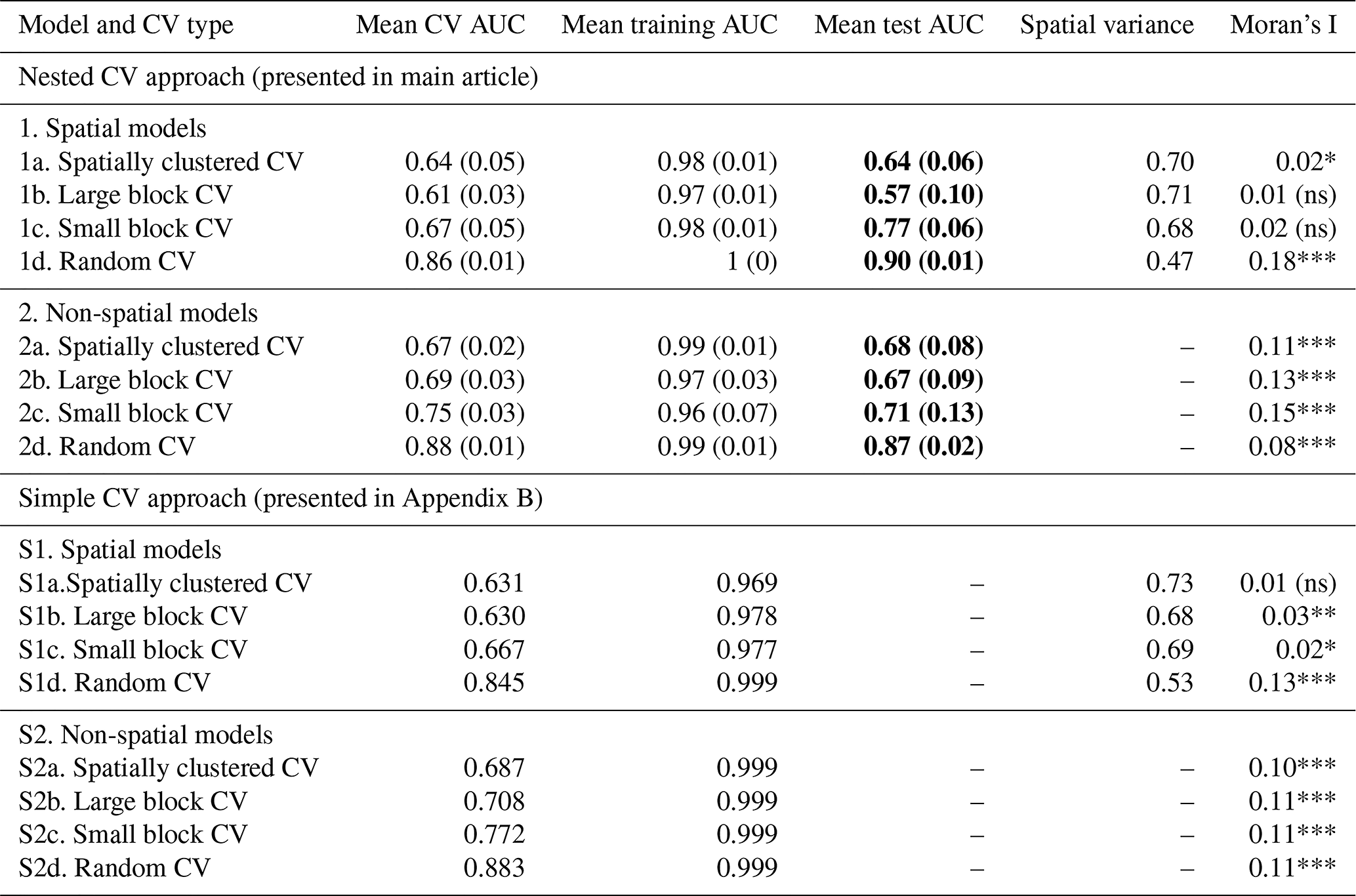
Table B2 Mean (and standard deviation) model performance metrics of two Gaussian Process Gradient Boosted classification models using four different cross-validation (CV) methods and two CV strategies (nested CV and simple CV) on the forest-only landslide dataset. AUC=area under the curve, where values close to 1 indicate near perfect accuracy of landslide/control point classification. Mean CV AUC=mean value from hyperparameter search (Step 4 in Fig. 3 and B1); Mean training AUC=mean value from inner loop training models (Step 5 in Fig. 3 and Final model in Fig. B1); Mean test AUC=mean value from testing inner loop models (Step 6 in Fig. 3) is shown in bold as it is the most useful metric for evaluating performance, but it is absent in the simple CV approach. Spatial variance indicates the amount of variance explained by the spatial structure of the model (absent from non-spatial models). The significance of the Moran's I test for spatial autocorrelation is indicated by asterisks ($***=p<\mathrm{0.001}$, $**=p<\mathrm{0.01}$, $*=p<\mathrm{0.05}$, ns=non-significant). A significant Moran's I indicates that residual spatial autocorrelation is likely. Note there are no standard deviation values for the simple CV, as the hyperparameter optimisation was completely internally and only one final model was constructed.

Appendix C

Figure C1 Spatial distribution of the folds assigned for the full models during (a) spatially clustered cross-validation, (b) large block cross-validation, (c) small block cross-validation and (d) random cross-validation.

Figure C2 Spatial distribution of the folds assigned for the forest-only models during (a) spatially clustered cross-validation, (b) large block cross-validation, (c) small block cross-validation and (d) random cross-validation. Note that the number of folds had to be reduced to three for large block CV and four for small block CV to create folds which contained a relatively balanced number of both landslide and control points.

Appendix D

Predictor correlation structure

To assess whether collinearity among predictors could explain differences in variable importance across modelling approaches, we computed pairwise associations for all predictors retained in the final model. Given the mixed measurement types in our predictor set, we used Spearman's rank correlation for continuous–continuous and continuous–ordinal pairs, the correlation ratio (η, derived from one-way ANOVA) for pairs involving a nominal categorical predictor and a continuous or ordinal predictor, and Cramér's V for pairs of nominal categorical predictors. Pairwise results are visualised separately for signed (Spearman; Figs. D1 and D3) and unsigned (η, Cramér's V; Figs. D2 and D4) measures to avoid conflating measures with and without a meaningful direction of association.

Figure D1 Spearman's rank correlation matrix for continuous and ordinal variables retained in the models for the full dataset. Correlations between −0.05 and 0.05 are not shown.

Figure D2 Heat map of associations between categorical variables and all other variables retained in the models using the full dataset. Values between the categorical variables are Cramer's V, and values between categorical and continuous/ordinal variable pairs are correlation ratio (η, derived from one-way ANOVA).

Figure D3 Spearman's rank correlation matrix for continuous and ordinal variables retained in the models for the forest dataset. Correlations between −0.05 and 0.05 are not shown.

Spatial autocorrelation of predictors

Tables D1 (for the full dataset) and D2 (for the forest-only dataset) summarise how strongly each predictor is spatially autocorrelated and how much of that autocorrelation remains under different cross-validation (CV) schemes.

Figure D4 Heat map of associations between categorical variables and all other variables retained in the models using the forest dataset. Values between the categorical variables are Cramer's V, and values between categorical and continuous/ordinal variable pairs are correlation ratio (η, derived from one-way ANOVA).

We quantified spatial autocorrelation in predictor variables by fitting spherical variogram models to each predictor using the observed spatial coordinates of all data points. Variograms with a nugget-to-sill ratio exceeding 0.6 were flagged and inspected visually, as such fits often indicate a predominantly unstructured (short-range) predictor for which a large apparent range is a fitting artefact rather than genuine long-range spatial structure. Those variables with a low nugget-sill ratio are those with a strong spatial structure which may not always be accounted for during CV processing. This is apparent when inspecting the residual correlation of each predictor at the held-out distance of each CV scheme. To derive this held out distance for each of the four cross-validation schemes evaluated in the main analysis (random, small block, large block, and spatially clustered), we computed, for every held-out observation, the Euclidean distance to its nearest training-set observation. We used the distribution of these nearest-neighbour distances as an empirical measure of the spatial independence enforced by each scheme, and as a scheme-specific reference distance against which to evaluate residual predictor autocorrelation. We then evaluated the fitted variogram model for each predictor at the median nearest-neighbour distance for each cross-validation scheme, converting the resulting semi-variance to an implied correlation. This provides a scheme-specific estimate of how much spatial correlation in a given predictor remains at the characteristic distance separating training and test observations under that scheme; and therefore, how readily that predictor could act as a spatial proxy (a source of information leakage) under random assignment.

Table D1 Summary of predictor spatial autocorrelation for full dataset. Effective range = distance at which spatial autocorrelation reduces to 0; Nugget = relative amount of random noise at distance 0; Partial sill = portion of variance explained by spatial structure; total sill = Total variance; Nugget to sill ratio = portion of variance explained by random noise: low values indicate a high level of spatial structure in the data. The last four columns give the autocorrelation coefficient value at the median train:test distance of the four CV methods. The median distances for the CV schemes are: Random = 882 m, Small block = 10 641 m, Large Block = 22 893 m, Spatial clustering = 22 766 m. Values and variables in bold indicate variables that should be viewed with caution. E.g. the spatial autocorrelation of Elevation remaining at the median distance between training points and testing points in the random CV scheme is 0.81. Therefore, the random CV method is unlikely to completely account for spatial autocorrelation in this variable.

Table D2 Summary of predictor spatial autocorrelation for forest dataset. Column heading definitions are given in the text. See above caption for column heading definitions. The median distances for the CV schemes are: Random = 1077 m, Small block = 10 820 m, Large Block = 25 893 m, Spatial clustering = 20 943 m. Values and variables in bold indicate variables that should be viewed with caution.

Appendix E

Here we present additional partial dependence plots for the top four variables in the non-spatial model with spatially clustered cross-validation on the full dataset (Fig. E1) and forest-only dataset (Fig. E2). And a third partial dependence plot summarises all forest predictors in the forest-only, non-spatial model with spatially clustered cross-validation (Fig. E3).

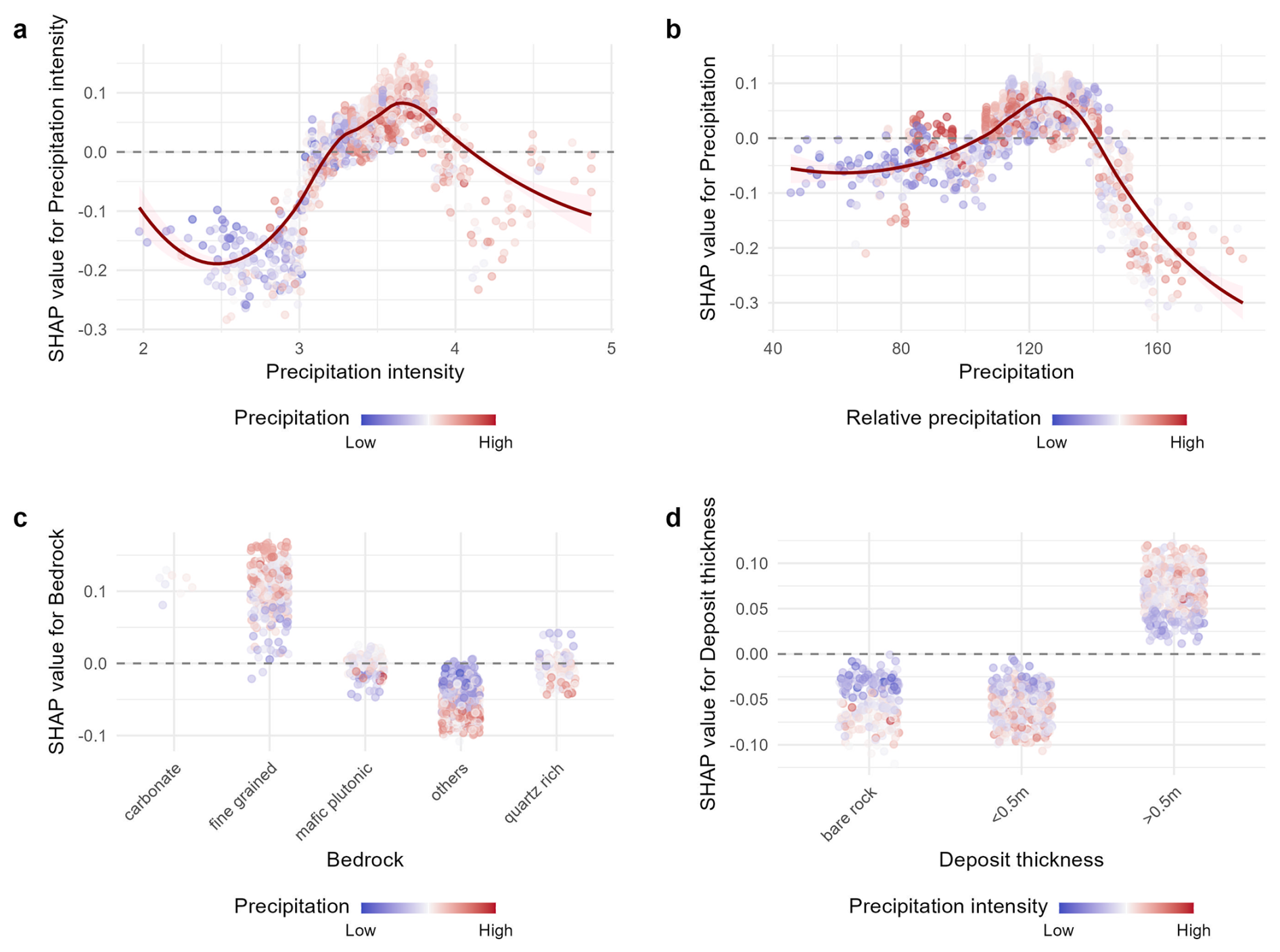
Figure E1 (a–d) Partial dependence plots for the top four variables of full model 2a (non-spatial model with spatially clustered CV). Precipitation intensity in (a) is square root transformed. Each point represents an observation and is plotted with its feature value on the x-axis and SHAP value (contribution to model output) on the y-axis. SHAP values above 0 indicate that a feature value is likely to make a positive contribution to the probability of a landslide. Points are coloured by a second feature chosen to minimise the variance of the SHAP value given both features and represents the strongest interaction. Solid red lines are LOESS smoothed lines and shading represents 95 % confidence intervals.

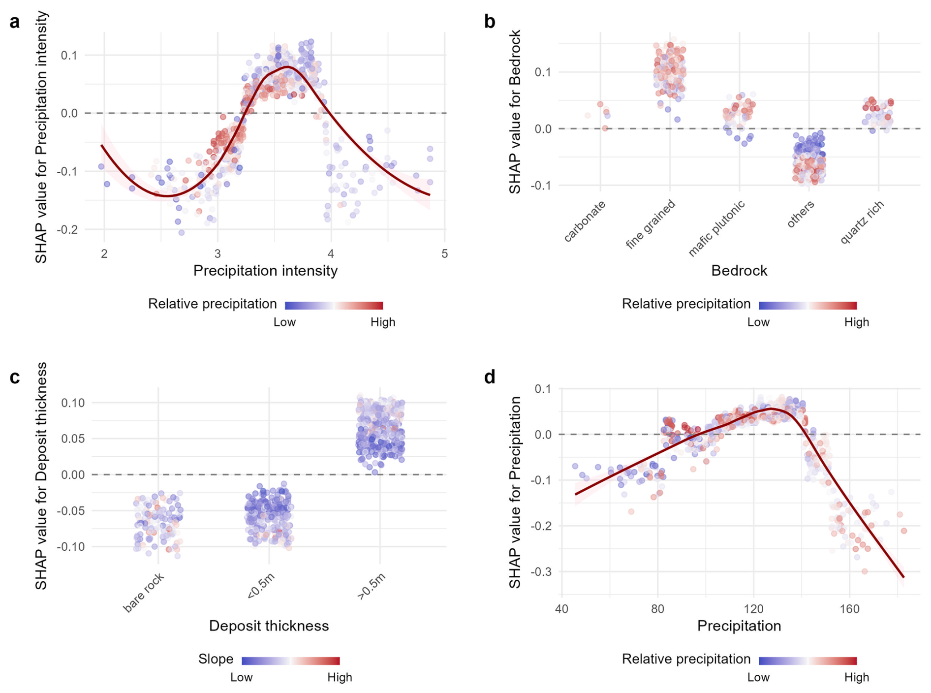
Figure E2 (a–d) Partial dependence plots for the top four variables of forest-only model 4a (non-spatial model with spatially clustered CV). Precipitation intensity in (a) is square root transformed. Each point represents an observation and is plotted with its feature value on the x-axis and SHAP value (contribution to model output) on the y-axis. SHAP values above 0 indicate that a feature value is likely to make a positive contribution to the probability of a landslide. Points are coloured by a second feature chosen to minimise the variance of the SHAP value given both features and represents the strongest interaction. Solid red lines are LOESS smoothed lines and shading represents 95 % confidence intervals.

Figure E3 (a–d) Partial dependence plots for the four included forest variables of forest-only model 4a (non-spatial model with spatially clustered CV). Each point represents an observation and is plotted with its feature value on the x-axis and SHAP value (contribution to model output) on the y-axis. SHAP values above 0 indicate that a feature value is likely to make a positive contribution to the probability of a landslide. Points are coloured by a second feature chosen to minimise the variance of the SHAP value given both features and represents the strongest interaction. Solid red lines are LOESS smoothed lines and shading represents 95 % confidence intervals.

Here we present additional SHAP value summary plots for all 16 nested CV models (Figs. E4–E7).

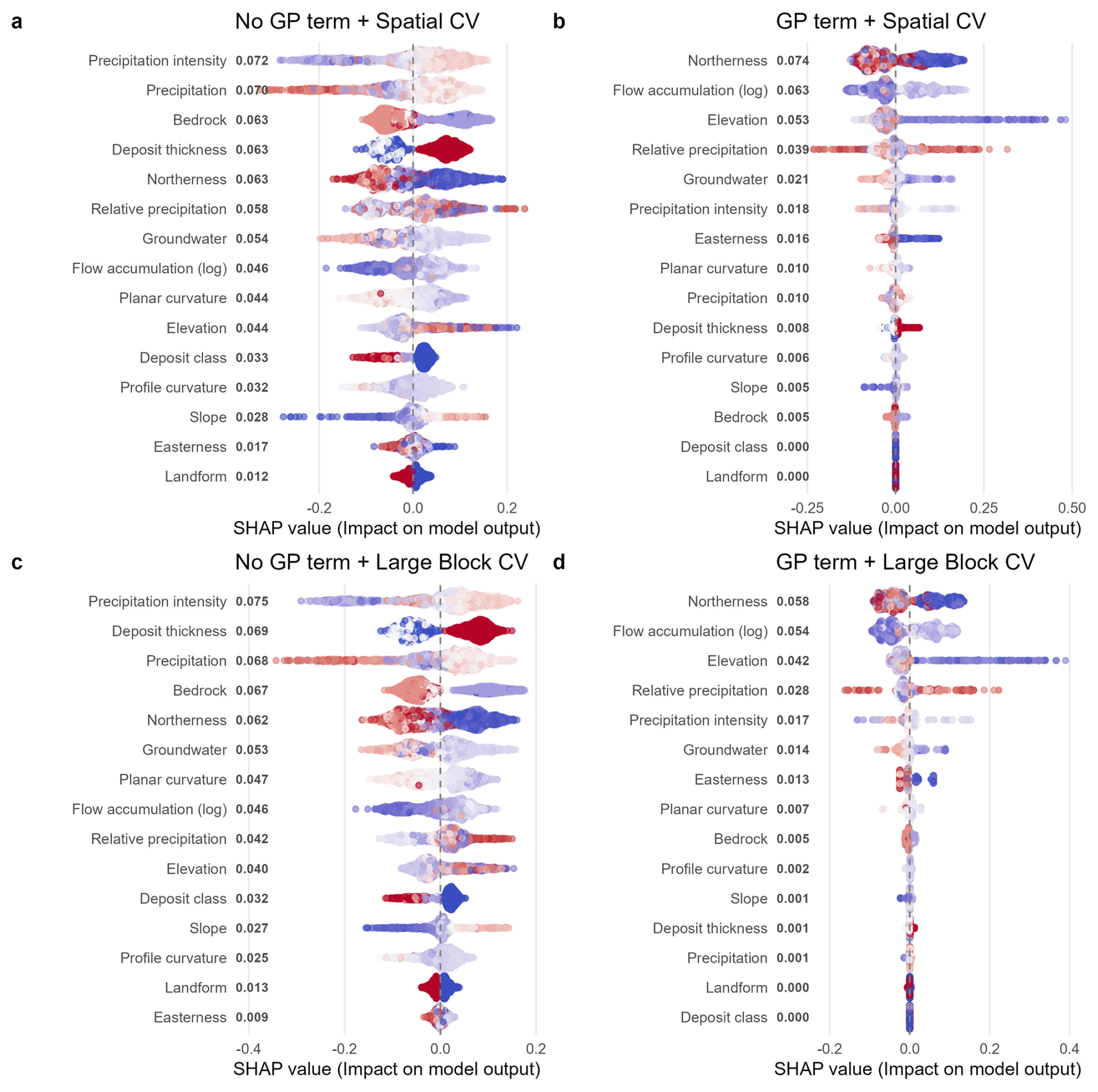
Figure E4 Shapley value summary plots for models on the full dataset (a) spatially clustered CV without a spatial term (model 2a), (b) spatially clustered CV with a spatial term (model 1a), (c) large block CV without a spatial term (model 2b) and (d) large block CV with a spatial term (model 1b) The numbers after variable names are mean absolute SHAP values, representing relative importance. Points are coloured by normalised feature value.

Figure E5 Shapley value summary plots for models on the full dataset: (a) small block CV without a spatial term (model 2c), (b) small block CV with a spatial term (model 1c), (c) random CV without a spatial term (model 2d) and (d) random CV with a spatial term (model 1d) The numbers after variable names are mean absolute SHAP values, representing relative importance. Points are coloured by normalised feature value.

Figure E6 Shapley value summary plots for models on the forest-only dataset: (a) spatially clustered CV without a spatial term (model 4a), (b) spatially clustered CV with a spatial term (model 3a), (c) large block CV without a spatial term (model 4b) and (d) large block CV with a spatial term (model 3b) The numbers after variable names are mean absolute SHAP values, representing relative importance. Points are coloured by normalised feature value.

Figure E7 Shapley value summary plots for models on the forest-only dataset: (a) small block CV without a spatial term (model 4c), (b) small block CV with a spatial term (model 3c), (c) random CV without a spatial term (model 4d) and (d) random CV with a spatial term (model 3d) The numbers after variable names are mean absolute SHAP values, representing relative importance. Points are coloured by normalised feature value.