Autonomous and efficient large-scale snow avalanche monitoring with an Unmanned Aerial System (UAS)

Current and accurate information about the location and extent of released avalanches is critical for public safety and decision-making. However, such data is difficult and expensive to obtain in remote locations. Uncrewed fixed-wing aerial vehicles, due to their low cost, long range, and high travel speeds, are promising platforms to gather aerial imagery to map avalanche activity. However, autonomous flight in mountainous terrain remains a challenge due to the complex topography, regulations, and harsh weather conditions. In this work, we present a proof of concept system that is capable of safely navigating and mapping avalanches using a fixed-wing aerial system (UAS) and discuss the challenges arising for operating such a system. We show in our field experiments that we can effectively and safely navigate in steep mountain environments while maximizing the map quality and efficiency while meeting regulatory requirements. We expect our work to enable more autonomous operations of fixed-wing vehicles in alpine environments to maximize the quality of the data gathered. By enabling the acquisition of frequent and high quality information on avalanche activity, such drone systems would have a large impact of safety critical applications such as avalanche warning, mitigation measure planning or hazard mapping.

1 Introduction

Spatially continuous documentation of hazardous natural processes such as snow avalanches, rockfalls, or debris flows provides critical information for risk management. Knowing the history – when, where, and under which conditions these processes have occurred helps to continuously assess and act upon risk levels of the hazard. For snow avalanches, the natural hazard claiming most lives in Switzerland on average (Schweizer, 2008), informed decision-making relies on the large-scale availability of, among others, the spatial extent and size of occurred avalanches. This data benefits applications including hazard mapping, mitigation measure planning and evaluation, risk analysis, avalanche warning, numerical avalanche models, as well as avalanche research.

However, as avalanches occur in remote and potentially dangerous locations, this data is difficult to obtain (Schweizer et al., 2021; Bühler et al., 2019). Consequently, available data sources are often limited to easy-to-access locations and events, leaving an incomplete and possibly biased state of information and understanding. Historically, avalanche data acquisition has relied on human observers, more recently complemented by stationary sensors like Doppler radars or infrasound (e.g., Schimmel et al., 2017) or remote sensing with satellites, airplanes or drones (e.g., Eckerstorfer et al., 2016; Hafner et al., 2023). Doppler radars and infrasound require in-situ infrastructure and only cover limited areas. Both optical (Lato et al., 2012; Bühler et al., 2019; Hafner et al., 2022) and synthetic-aperture radar (SAR) (Eckerstorfer et al., 2019; Leinss et al., 2020; Bianchi et al., 2021) from satellites have been successfully used to automatically detect avalanches over large areas. However, suitable satellite data can be expensive (e.g., Bühler et al., 2019), may lack the temporal resolution for monitoring (e.g., Hafner et al., 2022), may struggle with capturing smaller avalanches (e.g., Hafner et al., 2021) or in case of SAR, only capture parts of the avalanche (Eckerstorfer and Malnes, 2015; Hafner et al., 2021). Unlike satellite imagery, aerial imagery acquired with airplanes or drones allows for photogrammetric reconstruction of the surface which provides information on the snow (volume) distribution and the release height of avalanches in addition to the avalanche area from release to deposit (e.g., Bühler et al., 2015; Meyer et al., 2022; Bührle et al., 2023). However, crewed airplanes have high operating costs and limited deployment availabilities per season (Bühler et al., 2016).

Utilizing easily manageable small unmanned aerial systems (sUASs), also denoted as drones, could provide the benefits of using aerial imagery at a fraction of the cost of operating manned airplanes. The high speed (order of 5–30 m s⁻¹ ), long-range, and ability to be deployed with relatively little fixed ground infrastructure makes fixed-wing type sUASs particularly well-suited to capturing remote imaging data over hard-to-access areas. sUASs have already proven their usefulness in various applications for large-scale environmental monitoring (Lin and Lee, 2008; Astuti et al., 2009; Vivaldini et al., 2019; Shah et al., 2020; Islam and Hu, 2021; Jouvet et al., 2019; Teisberg et al., 2022).

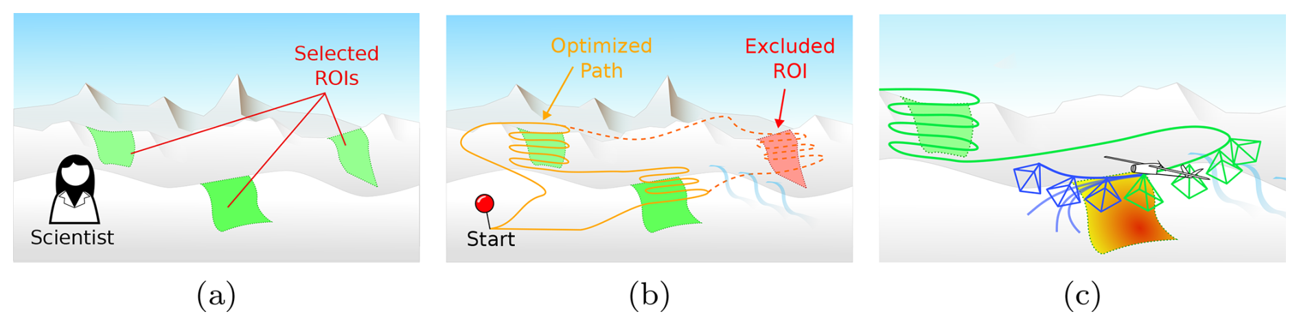
Figure 1 Overview of the autonomous avalanche monitoring using a long-range fixed-wing UAV. (a) Scientific domain expert defines multiple ROIs which can be avalanche release areas. (b) A subset of reachable ROI would be selected for a single sortie and passed to the small uncrewed aerial system (sUAS) (c) Once reaching the ROI, the vehicle will gather image data for use of photogrammetry where the release volume, avalanche outline and texture of the snow can be acquired.

We envisage the data-collection process for avalanches by collecting remote imaging data with an sUAS. An sUAS capable of autonomously traveling long distances to reach multiple remote interest areas, mapping the avalanche release area, and safely returning to the start location would provide high-quality avalanche distribution data with accurate release volume estimates. The envisioned workflow would be as follows. In the first stage, one or multiple target region of interests (ROIs) would be pre-selected by a domain expert operator with an understanding of the conditions that are most likely to cause avalanche events (Fig. 1a). Alternatively, modeled avalanche terrain (e.g., Bühler et al., 2022) could be used. Next, a subset of reachable ROIs would be selected for a single sortie, and passed to the sUAS (Fig. 1b). On reaching the ROI, the vehicle gathers image data autonomously for photogrammetry and ensures that the gathered images produce an accurate reconstruction (Fig. 1c). Once all the image data is acquired, the vehicle should safely return to the launch site. The photogrammetrically processed data can then be used to determine the release and deposit height, release volume, avalanche area, and snow depth distribution.

Executing such a mission with an sUAS first requires a route optimization method to determine which ROIs fit within a single sortie. Then, the vehicle should be capable of navigating safely towards the ROI, efficiently map the avalanches, and finally move to the next ROI or return to the launch location. Due to the finite image resolution, vehicles might need to fly close to the snow surface in order to acquire image data with the necessary ground sample distance (GSD). Moreover, current regulations applied in the EU and Switzerland (European Commission, 2019) require the vehicle to maintain a close distance to the terrain. However, operating fixed-wing aerial vehicles in steep alpine environments remains a major challenge as they operate at high speeds and are severely limited in maneuverability. This increases the risk of the vehicle entering an unsafe state, as the terrain might become steeper than the vehicle can climb, or narrower than the vehicle can turn (Lim et al., 2024a). The presence of mountain forests at steep slopes with trees of up to 35 m height above ground further reduces airspace margins and increases the probability of crashing. Additionally, state-of-the-art image data-gathering surveys are pre-planned using a sequence of automatic or handcrafted waypoints. However, these methods struggle to ensure safe and regulation-compliant operations for fixed-wind sUASs, especially in steep alpine terrain. Furthermore, pre-planned surveys are unable to account for interferences such as wind gusts, that disturb the different viewpoints away from those planned, potentially resulting in poor or incomplete reconstruction.

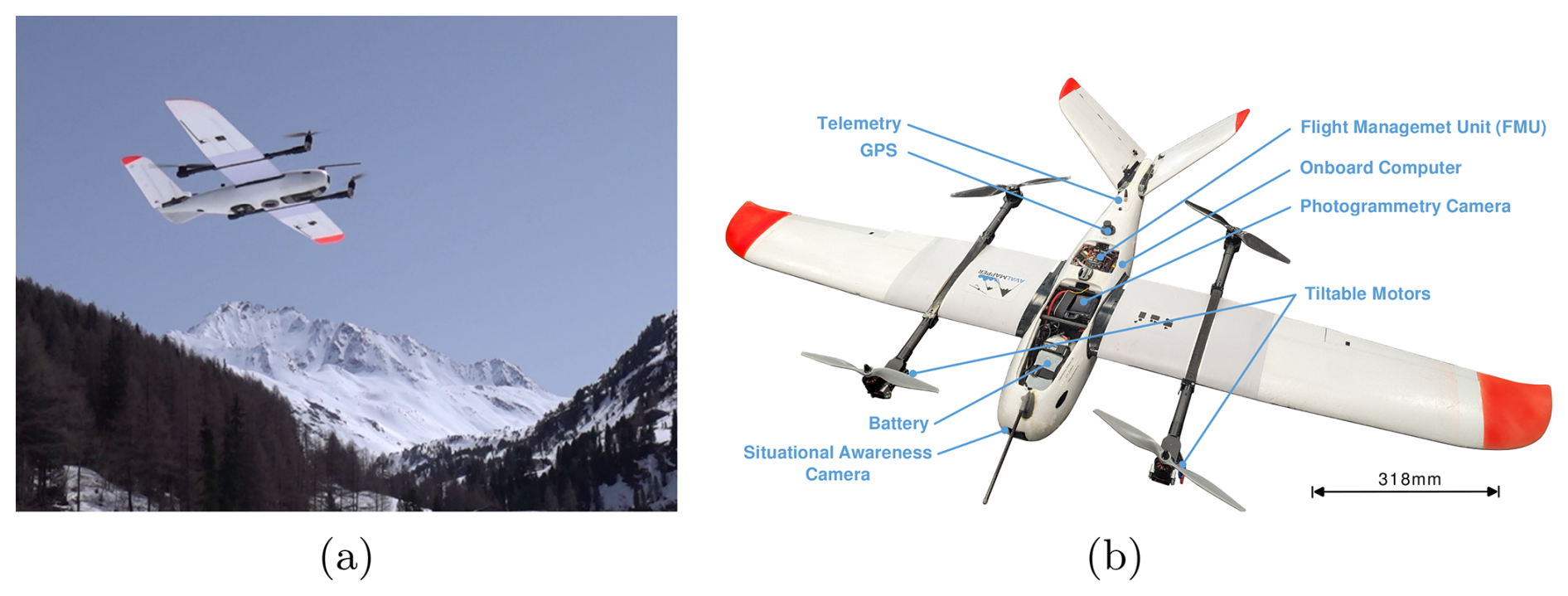
Figure 2 (a) Image of the tiltrotor VTOL platform taking off during the field deployment in a narrow valley in Davos, Switzerland. (b) Overview of airframe and components of the system.

In this paper, we address these challenges using an autonomous planner capable of navigating in steep mountainous terrain and autonomously mapping the terrain surface for photogrammetry reconstruction. As the vehicle is operated autonomously, there is no longer a need to explicitly pre-plan the mission, allowing the operator to dynamically change the behavior during flight. This can be useful to adjust the vehicle's mission depending on changing situations, such as weather conditions, which is not possible with conventional pre-planned missions. The vehicle navigates to the ROI autonomously using a safe path planner. Then, the system collects high-quality photos by actively optimizing viewpoints during flight for reliably creating a photogrammetric reconstruction of the terrain. This work integrates recent advances in fixed-wing navigation and mapping (Lim et al., 2023b, 2024a, b) into an integrated system for avalanche mapping. We demonstrate and evaluate the approach by deploying an integrated tiltrotor vertical takeoff and landing (VTOL) system in alpine terrain in Davos, Switzerland (Fig. 2). Ultimately, our work is a step towards a fixed-wing sUAS that can autonomously map avalanches.

2 Prior Work

2.1 Environmental Monitoring with sUAS

Easily manageable sUAS have become a data collection tool for environmental (Dunbabin and Marques, 2012),hazard and disaster monitoring (Gomez and Purdie, 2016). Especially, multirotor type sUAS are popular, due to their mechanical simplicity, agile flight characteristics, and minimal requirements for ground infrastructure. However, multirotor type sUAS are not energy efficient, limiting their range and flight time, and therefore not well-suited to large-scale environment monitoring tasks. In contrast, fixed-wing type sUAS are more efficient, with long range and fast cruise speed, which are well suited for large-scale environment monitoring tasks. Therefore, fixed-wing type sUAS have been used for large scale environment applications such as hurricanes (Lin and Lee, 2008), volcanoes (Astuti et al., 2009) and forests (Vivaldini et al., 2019).

In alpine environments, sUAS has been used for snow depth mapping (Vander Jagt et al., 2015; Harder et al., 2016; Bühler et al., 2016, 2017; De Michele et al., 2016) or monitoring glaciers (Jouvet et al., 2019; Teisberg et al., 2022). Bühler et al. (2016) showed that using photogrammetry with a camera mounted on an sUAS can provide high-quality snow depth data. However, homogeneous snow texture remains a significant challenge due to a lack of distinct visual features required for reconstruction (Bühler et al., 2017). Captured avalanches can be easily mapped manually (Bühler et al., 2019) or semi-automatically (Hafner et al., 2022) from the generated orthophotos. Outlines mapped from georeferenced data contain an existential uncertainty as different human experts map the avalanches slightly differently, but they lack the positional uncertainty inherent to avalanches mapped from the ground (Hafner et al., 2023).

However, most of the previous approaches rely on preplanned paths that are carefully hand-designed using a sequence of waypoints. This requires expert planned missions which may be hard to dynamically alter during operations, making it difficult to ensure safe operations when something unforeseen changes. Additionally, the tight altitude constraints (120 m above ground level (a.g.l.)) posed by the EU regulations (European Commission, 2019) pose a significant challenge in planning a safe mission, as the vehicle's deviation from the waypoint sequences is hard to predict. In this work, we use an autonomous planner that does not require explicit waypoint planning but rather is directly constrained by the digital elevation map (DEM) and can autonomously steer the vehicle during flight. Also, provided with the target ROI, the planner dynamically adapts to the actual measurements to ensure good quality of the photogrammetry reconstruction.

2.2 Navigation with Fixed-wing Aerial Vehicles

Like birds, fixed-wing vehicles leverage the aerodynamic lift generated by their wings to stay airborne. As this is an energy-efficient way to generate the lift force required to stay airborne, fixed-wing vehicles can for fly longer than other types of aerial systems. However, generating sufficient aerodynamic forces requires the vehicle to maintain a high speed relative to the air. High speed limits spatial maneuverability, imposing constraints such as minimum turn radius or maximum flight path angle (Chitsaz and LaValle, 2007). Most importantly, fixed-wing vehicles cannot stop, as opposed to other types of vehicles such as multirotor or helicopter-type vehicles that can hover in one position. This property of fixed-wing vehicles poses a significant challenge in ensuring safety when operating in complex environments (such as mountainous regions), where the terrain can be either steeper than the vehicle can climb or the valley narrower than the vehicle can turn (Lim et al., 2024a). This can lead to the vehicle entering an inevitable collision state (ICS) (Fraichard and Asama, 2004), a state where there are no feasible actions that the vehicle can take to avoid an eventual collision, in particular with trees. Such occurrences of ICS can be challenging for the operator to correct, as the vehicle may enter an ICS long before an actual collision occurs. Practical implementations of fixed-wing path planning have been shown in indoor (Bry et al., 2015) and alpine environments (Oettershagen et al., 2017; Duan et al., 2024b), using curvature constrained Dubins curves (Dubins, 1957; Owen et al., 2015) to represent the maneuverability constraints of fixed-wing aerial vehicles. However, these approaches only find collision-free paths without considering safety against entering an ICS. Additionally, the vehicle needs to consider constraints imposed by the regulations, such as the EU altitude restrictions (European Commission, 2019) that limit flight to below 120 m a.g.l.

In this work, we built on previous work from Lim et al. (2024a) which utilizes periodic circular loiter paths to simplify the evaluation of safety directly on a DEM. To integrate the planner into the system, we incorporate the safe path planner into a finite state machine, so that the vehicle always remains in a safe state. While the operator can modify the target position or path, the vehicle cannot enter an unsafe maneuver. This provides the flexibility to dynamically adjust the flight plan while guaranteeing safety and compliance with the tightened regulations.

2.3 Active Mapping for Aerial Photogrammetry

The most widely used method to plan a photogrammetry mission for an aerial vehicle is by generating a coverage pattern that covers the ROI with a specified GSD (the target size of an image pixel projected on the ground) and amount of image overlap (Galceran and Carreras, 2013). One common approach to generate a coverage pattern is boustrophedon (“the way of the ox”) decomposition (Choset, 2000). First, the target region is divided into a set of non-overlapping convex polygons (whose union is the complete target region). Next, for each polygon, the algorithm generates a sweep pattern (commonly known as boustrophedon or “lawn-mower”) consisting of parallel alternating-direction straight line segments, separated by a fixed distance based on the desired sensor footprint and overlap. Connecting the individual coverage patterns with transit segments results in a complete coverage path, ensuring that all parts of the target region are observed by the sensor. Extensions of this work can be found in decomposing nonconvex regions and planning the visit sequence as a traveling salesman problem (Bähnemann et al., 2021), or using Reeb graphs (Mannadiar and Rekleitis, 2010).

While this may be near-optimal for 2D planar environments (Choset, 2000), naïvely projecting the path over three-dimensional environments can result in inconsistent overlaps and ground sampling distances. Moreover, kinematically-constrained vehicles, such as fixed-wing vehicles, may struggle to follow the coverage patterns resulting in suboptimal performance (Mier et al., 2023). Therefore, boustrophedon decomposition-based coverage planning for fixed-wing vehicles requires significant engineering effort to work reliably in steep alpine environments. Further, preplanned missions are less robust against environmental disturbances such as wind, where aircraft motion may result in the actual image poses deviating from the planned poses. Since the plan is not adjusted for these disturbances during execution, the resulting image set may have holes and/or overly-covered regions (Coombes et al., 2017). A common strategy to address these issues is to generate overly conservative plans that enforce more image overlap than is required, in the hope that the minimum requirement is met when the plan is executed. However, there is no way to determine the quality of the image data gathered from the survey, making it hard for operators to judge whether the data quality is sufficient without running a time-consuming photogrammetric reconstruction.

Active view planning methods, on the contrary, plan future viewpoints iteratively based on previous observations. In a photogrammetric reconstruction context, active view planning involves selecting viewpoints that are most likely to improve the reconstruction given the previously collected views. A “good” image is one that helps ensure the target region is covered by multiple views from multiple directions. Explore-and-exploit methods (Morilla-Cabello et al., 2022; Hepp et al., 2018b; Bircher et al., 2016) evaluate the quality of the photogrammetric reconstruction to plan future viewpoints. However, these approaches use photogrammetric reconstruction between surveys to evaluate the quality of the reconstruction. As photogrammetric reconstruction is a computationally intensive operation, the limited payload and power available on an sUAS makes explore-and-exploit approaches challenging to use for maneuver planning during flight. Additionally, the dynamic nature of avalanches and short flight-weather windows make this approach impractical for avalanche monitoring. Some approaches use a lower computational cost view utility heuristic to estimate the quality of the target surface without reconstruction (Smith et al., 2018; Peng and Isler, 2018). Prior works have tried estimating the view utility metric through learning (Hepp et al., 2018a; Liu et al., 2022). However, these heuristics do not generalize well to different applications.

In our prior work (Lim et al., 2023b), the quality of reconstruction is estimated using Fisher information, derived from the measurement model of the camera. This makes the approach more generally applicable and less sensitive to heuristic parameters. In this work, an example of view planning was demonstrated by exhaustively searching over all possible maneuvers. However, due to the high branching factor, this is too computationally expensive to evaluate in real time. Therefore, we use a sampling-based approximate graph search such that the informative maneuvers can be computed onboard the vehicle in real time. Greedily selecting the next best single reachable view performs poorly for an aerial vehicle, because such a myopic sampling strategy may not allow the vehicle to reach more distant but highly informative viewpoints.

3 System Overview

We propose a system that is capable of autonomously navigating alpine environments and mapping a ROI without a handcrafted predefined plan, specifically developed for this project. We break down the system by route optimization, platform, autonomous planner, and operational processes. The route optimization determines the route on which ROI is feasible to visit within a single sortie. The platform includes the airframe hardware and avionics of the vehicle. The autonomous planner is the software running on the onboard computer that enables autonomous operations of the vehicle. Lastly, the operational process is presented to provide insight into the reduced workload of the operator during autonomous operations.

3.1 Route Optimization

We assume a situation in which an avalanche expert specifies a set of target regions to visit. These could be areas where avalanches have or are expected to have occurred, and the approximate location is known to the domain expert. With a large number of ROIs, or large ROIs, the vehicle may not be able to visit all the ROIs within a single sortie since the range of the vehicle is limited. Moreover, the large uncertainty in wind conditions introduces uncertainties on the reachability of ROIs accessible by the vehicle. The goal of the route optimization is to find a sequence of paths that maximizes the number of ROIs the vehicle can visit while ensuring that the vehicle can return to the goal point within a single sortie. If necessary, the route optimization is repeated sequentially, in order to cover all ROIs over multiple flights.

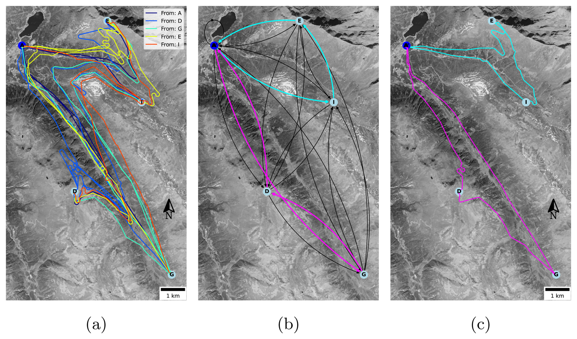
Figure 3 Visualization of the route optimization example with four ROIs. The start position is labeled as A, and the ROIs are labeled as D, G, E, I. (a) Roadmap of the full graph. Each edge is a safe path navigating from one vertex to the other. The edges are colored based on which vertex the edge is started from. (b) Graph and solution of the orienteering problem. The edge cost of the graph is the path length of the paths shown in the roadmap. The solution route of the orienteering problem is highlighted in cyan for the first flight, and magenta for the second flight. (c) Path of the solution path. Source of orthoimage: swisstopo (1998b).

In this work, we consider a realistic example of four ROIs that are distributed in the avalanche hazard area next to Davos, Switzerland (Fig. 3). We consider an energy budget based on the platform mentioned in Sect. 3.2, which is equipped with a 6S 23000 mAh lithium polymer battery. The route optimization problem for a single sortie can be formulated as an orienteering problem (Chao et al., 1996) and interpreted as a graph. For the graph, each ROI vertex is assigned a reward (the value of mapping that ROI) and a mapping cost (the approximate distance required to map the ROI), and each edge is assigned a traversal cost. The goal of the orienteering problem is to find a path from the start vertex to the goal vertex, visiting the set of ROI vertices that maximizes the number of ROIs visited, while keeping the total cost (or, effectively, the energy spent) within the limited energy budget. For a realistic long-range deployment scenario considered in this paper, we assume the start and end vertices to be at the same location.

To construct the graph, edges are generated by finding the shortest path between the ROI positions (Fig. 3a). Each ROI position is considered as a loiter path, which is used as an intermediate position to start mapping the ROI and return to before navigating to the next ROI. If a path exists between all nodes, we can consider the graph as a fully connected graph (Fig. 3b). A sampling-based path planner that considers the kinematic constraints of a fixed-wing vehicle, while staying under the constraints of distance to terrain remaining between 50 to 120 m is used for generating the edge (Lim et al., 2024a). Note that the edges are directional and asymmetric, meaning that the cost of navigating between two nodes depends on the direction of travel. We consider the expected energy required to traverse the path using the model in Duan et al. (2024a) to be the cost of the edge (Fig. 3b). The energy model accounts for the 3D geometry of the path as well as wind. Therefore, the edge costs can be updated based on wind conditions, if available. In this work, however, we assume zero wind, noting that accurate local, low-altitude wind-estimates are very challenging to obtain, especially in the considered terrain. To accommodate the respective uncertainty, we instead plan with a conservative energy budget for simplicity.

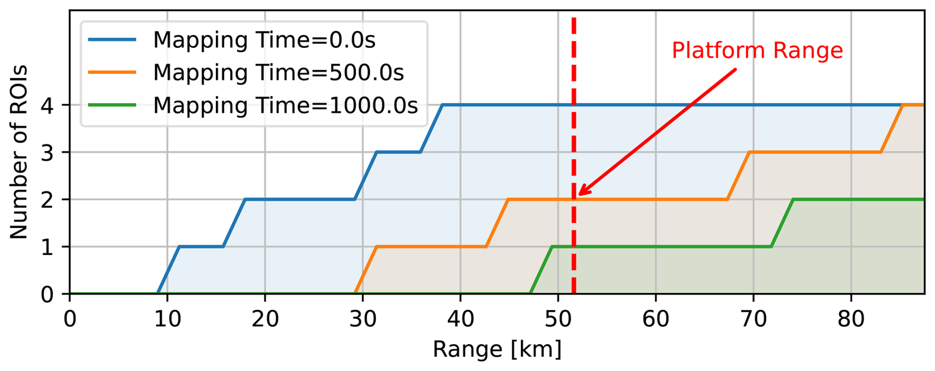
Figure 4 Number of ROIs reachable with different ranges of the vehicle, for the ROIs shown in Fig. 3a. Low mapping time allows the vehicle to reach more ROIs. The range of the platform (51.6 km) is marked as the red dotted line.

To solve the orienteering problem, we use the branch-and-bound method, a graph search algorithm that reduces the search space by pruning the decision tree that is not promising (Land and Doig, 2010). The orienteering problem is applied sequentially over multiple flights, until all ROIs are covered with each sortie. In the example we assumed each sortie has the same energy budget, e.g. fully charged batteries. The solution path for the orienteering problem can be found on the graph highlighted in cyan (Fig. 3b), and the path extracted from the roadmap to create a plan (Fig. 3c).

In order to compare the impact of range for gathering sufficient information, we compare the number of ROIs the vehicle would be able to visit and map, to the range of the vehicle (Fig. 4). The range is calculated based on level flight with cruise airspeed (18.7 m s⁻¹). Additionally, we compare the number of ROIs that the vehicle can visit for the first sortie, depending on the average mapping time to map an ROI. It can be seen that multirotor vehicles, which have a typical range of 10–15 km would not be able to visit and map a single ROI in this example, even if we were to ignore the cost to map the ROI (mapping time = 0 s). Therefore, fixed-wing aerial vehicles, which typically have a much longer range, would be better suited for visiting multiple ROIs. Additionally, we can see that the time required for mapping has a significant impact on the number of ROIs the vehicle can visit. In our example, the range of the platform is around 51.6 km and the vehicle would only be able to visit all four ROIs if it does not need to spend any time for mapping. In contrast, if the average mapping time is been raised to 1000 s, the platform will only be able to visit one ROI. This underlines the importance of an efficient mapping method. Active mapping, as we propose in this work, helps to reduce the mapping cost, allowing the vehicle to visit more ROIs within a single sortie. The route plan optimized with an average mapping time of 500 s shows that we need to perform sequential missions to cover all four ROIs (Fig. 3a) and the path can be extracted from the graph optimized through solving orienteering (Fig. 3b).

Note that validating the route optimization for several ROI on a real platform would require beyond visual line of sight (BVLOS) flight operations. Therefore, we exclude this from the field test evaluations presented in Sect. 4, and demonstrate only with a single ROI.

3.2 Platform

The platform consists of the airframe and the avionics system. The airframe is a commercially-available tiltrotor VTOL aircraft with a mass of 5.7 kg and a wingspan of 2300 mm based on the Makeflyeasy Freeman (mfe, 2024) (Fig. 2b). The wing-mounted motors tilt upwards to hover during takeoff and landings, which eliminates the need for a runway and allows the vehicle to launch and land in confined locations. This is a significant advantage in mountainous environments where flat regions large enough for traditional fixed-wing take-off can be hard to find. After take-off, the front rotors tilt forward to operate as a normal fixed-wing vehicle for the remainder of the mission until landing. The fixed-wing flight modality uses 9.5 % of the power compared to hovering flight, and cruise speed of 18.7 m s⁻¹, extending the range of the system significantly. We assume that the vehicle always maintains the air-relative cruise speed such that the vehicle maximizes its endurance, and simplifying the planning process.

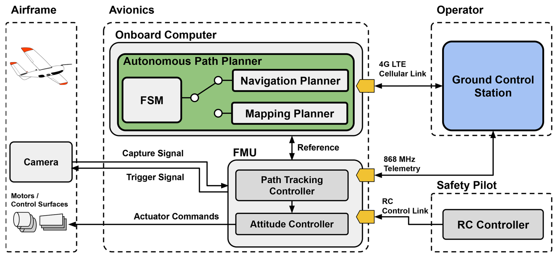
Figure 5 Overview of the autonomous avalanche monitoring flight system. The system consists of a mission computer and an FMU which are controlled by an operator and a safety pilot.

The avionics of the system consist of a flight management unit (FMU) and an onboard computer. Our system uses the Holybro Pixhawk 4 FMU running the PX4 autopilot software (Meier et al., 2015). The FMU runs low-level control loops, such as the guidance controller used for path following (Stastny and Siegwart, 2019), which stabilize the vehicle and is capable of global navigation satellite system (GNSS)-based navigation. GNSS-based navigation provides safety in case the onboard computer fails or the communication to the operator or safety pilot is lost. The onboard computer is an Intel NUC, equipped with a 3.5 GHz Intel Core i7-7567U CPU. When engaged, the computer runs the autonomous path planner, sending commands to the FMU.

The vehicle is operated through an operator using two independent communication links. A cellular connection to the onboard computer is used for command and visualization of the autonomous planner, as well as telemetry data directly from the FMU. A redundant 868 MHz telemetry connection is used to stream data directly from the FMU. An RC uplink enables a safety pilot to fly the vehicle manually in the case of an emergency.

The imaging payload is a 61 MP Sony A7R mirrorless camera mounted rigidly to the fuselage. To use the image data for photogrammetry, the FMU provides the camera with a capture trigger signal to acquire accurate timestamps for geotagging. A real time kinematic (RTK) GNSS is used for global position estimation, where the vehicle's global position is estimated by fusing inertial measurement unit (IMU) data. The image data is geotagged post-flight by synchronizing the capture signal to the image sequences. On the ground, the geotagged images are passed to the photogrammetry reconstruction using Agisoft metashape (Agisoft, 2024a, b).

3.3 Autonomous Path Planner

We present an autonomous planner that is capable of safely guiding the fixed-wing aerial vehicle to the region of interest, autonomously mapping the avalanche, and returning to the takeoff position. Different tasks are executed through a finite state machine, which is shown in Fig. 6. The finite state machine allows the operator to change the behavior of the vehicle during the execution of the mission, without specifying low-level commands such as waypoints. This approach reduces the operator's workload, as the operator does not need to specify the exact waypoints and evaluate whether the mission plan is safe.

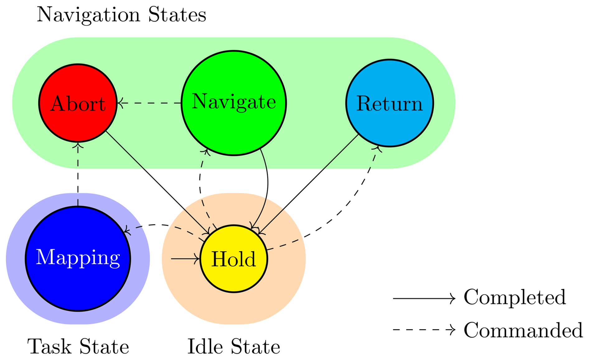
Figure 6 Finite state machine of vehicle operations. Dotted transitions are triggered by the operator, and the solid transitions are triggered upon task completion of the state.

There are five discrete states, denoted Hold, Navigate, Mapping, Abort, and Return. These states correspond to the respective tasks, which we group into an idle state, a navigation state, and a task state. An idle state includes the Hold state, where the vehicle stays on a circular periodic path. The vehicle can indefinitely wait for the next operator command, and therefore it is assumed that the vehicle always start from a Hold state. Navigation states include Navigate, Abort, Return, where the goal is to guide the vehicle safely to a target position from the current position. The task state includes the Mapping state, as this is the only task that the vehicle needs to do for data gathering. During Mapping state, the vehicle actively maneuvers to find the most informative set of viewpoints for photogrammetric reconstruction.

In all states, the path planner generates a reference path, which is a Dubins airplane path (Chitsaz and LaValle, 2007), consisting of a sequence of arc or line segments. Each segment of the reference path is represented as a geometric curve defined by its start position, length, and curvature. Each of the segments can be followed by the guidance controller, where the mission computer continuously sends path-tracking reference commands by computing the closest point p from the vehicle on the path, and the tangent t and curvature κ at the closest point. The reference command $\mathbf{r}=[\mathbf{p},\mathbf{v},\mathit{\kappa }]$ is sent to the FMU at 10 Hz. The reference commands are passed to a nonlinear path-following guidance controller based on Stastny and Siegwart (2019), which is robust against high wind conditions that can be found in alpine environments.

3.3.1 Safe Navigation

The goal of the navigation states Navigate, Abort, and Return, is to safely guide the vehicle to a target position from the current vehicle position subject to distance constraints relative to the terrain. The flying space is constrained by a minimum and maximum distance to a given DEM. To comply with the EU regulations, the vehicle needs to stay within 120 m distance from the terrain (European Commission, 2019). To ensure safety below, we additionally keep a minimum safety distance to the terrain to account for vegetation and artificial objects that are not present in the DEM (Fig. 7a).

The main challenge of the path planner is evaluating the safety of the path. In alpine environments, the terrain can be steeper than the vehicle's climb and turn limits. This is compounded by the narrow flyable space, between the maximum and minimum AGL constraints. In this setup, the state can enter an ICS (Fraichard and Asama, 2004), from where the vehicle may no longer be able to avoid a collision with the constraints. However, evaluating whether a state is an ICS requires infinite horizon collision checks, which is not practical (Fraichard and Asama, 2004; Bekris, 2010). To address this problem, we use the approach from Lim et al. (2024a), where periodic paths are evaluated with a DEM to simplify ICS checks. Periodic paths are useful for approximating an ICS checks, as a collision-free path for a single period can be considered collision-free for infinite cycles. Therefore, an infinite horizon collision check can be approximated much more efficiently.

In this work, we use a circular loiter pattern, which defines a safe periodic path because a fixed-wing aircraft can (ignoring energy constraints) safely fly in a fixed circular pattern indefinitely. Extending this, any path that does not intersect with the terrain, lies fully within altitude constraints, and ends on a safe circular trajectory also cannot contain an ICS and is therefore safe. In order to efficiently compute the safety of a loiter path, we define a valid loiter region, which are 2D positions of loiter centers where a circular loiter path exists within the AGL constraints (Fig. 7b). The valid loiter region is computed prior to the flight using the DEM, such that it can be evaluated quickly during the flight.

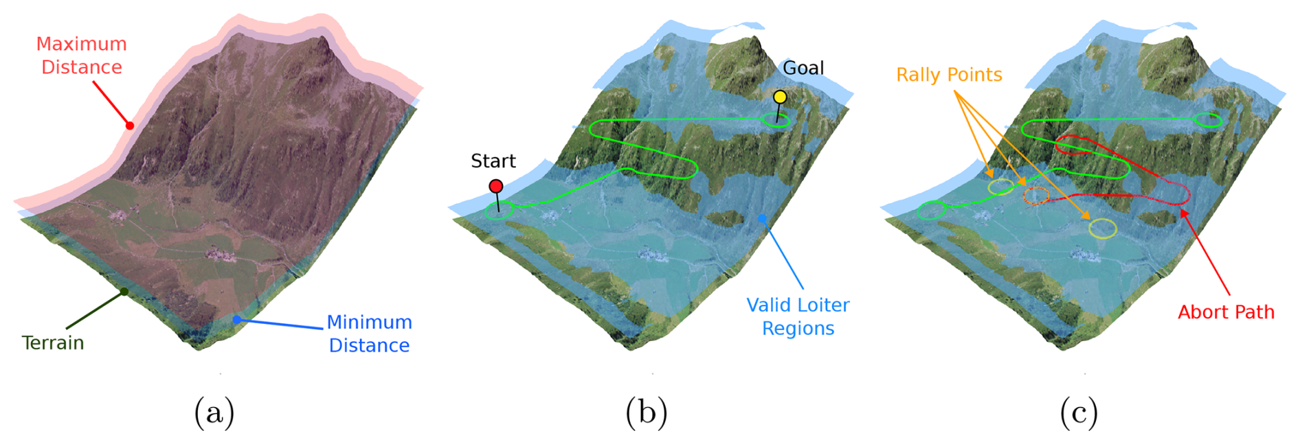
Figure 7 Visualization of the path planned by the navigation planner. (a) The terrain used for the example, where the red and blue overlay show the minimum and maximum distance constraints of 50 to 120 m a.g.l. (b) Shows the planned path in the Navigate state, where the path is planned from a start loiter to target loiter position. The light blue represents the Valid Loiter regions. (c) Shows the planned path in the Abort State, where the abort path is marked as red. The candidate loiter rally points are visualized in yellow. Source of DEM: swisstopo (1998a). Source of orthoimage: swisstopo (1998b).

Once the target loiter circle is evaluated to be inside the valid loiter region, a path planner is used to discover a safe path connecting the start and target loiter circle while respecting the kinematic constraints of the fixed-wing vehicle. We use a sampling-based path planner from Lim et al. (2024a), which uses RRT^* (Karaman and Frazzoli, 2010) with a metric defined by the Dubins airplane model (Chitsaz and LaValle, 2007) to approximate the kinematic constraints of the vehicle, where the kinematics is constrained with minimum curvature and flight path angle. A corrected Dubins set classification method (Lim et al., 2023a) is further employed to speed up the Dubins curve computation. While each of the navigation states (Navigate, Return, Abort) utilizes the same path planner, they differ in how the goal and start states are defined.

For the Navigate state, the operator specifies the target position. The target position is first checked for whether it lies in a valid loiter region. If the target position is valid, a path from the start loiter to the goal loiter is planned using the path planner(Fig. 7b). The start loiter path is defined as the loiter path the vehicle is already on. The same process applies to the Return state, except that the target loiter path is defined as the launch position.

Lastly, the Abort state is used for aborting a currently executed path. To identify a safe place to abort the current executed path, multiple positions within a specified radius are sampled. If a sampled position is in the valid loiter region, then it is considered as a rally point, where the vehicle can abort the mission safely. In this work, we search the terrain within a given radius until N valid rally points are discovered. If a valid path is found to one of these rally points, that path is executed. In this work, we found N=3 to be sufficient for finding a valid rally point (Fig. 7c).

3.3.2 Active Mapping

During the Mapping state, the active mapping planner guides the vehicle to acquire viewpoints that cover the ROI and that are expected to produce a high-quality photogrammetry reconstruction. The operator engages the Mapping state from a Hold state, where the loiter path should be placed close to the ROI. Once the mapping is complete, the termination of mapping is triggered by the operator by transitioning to the Abort state.

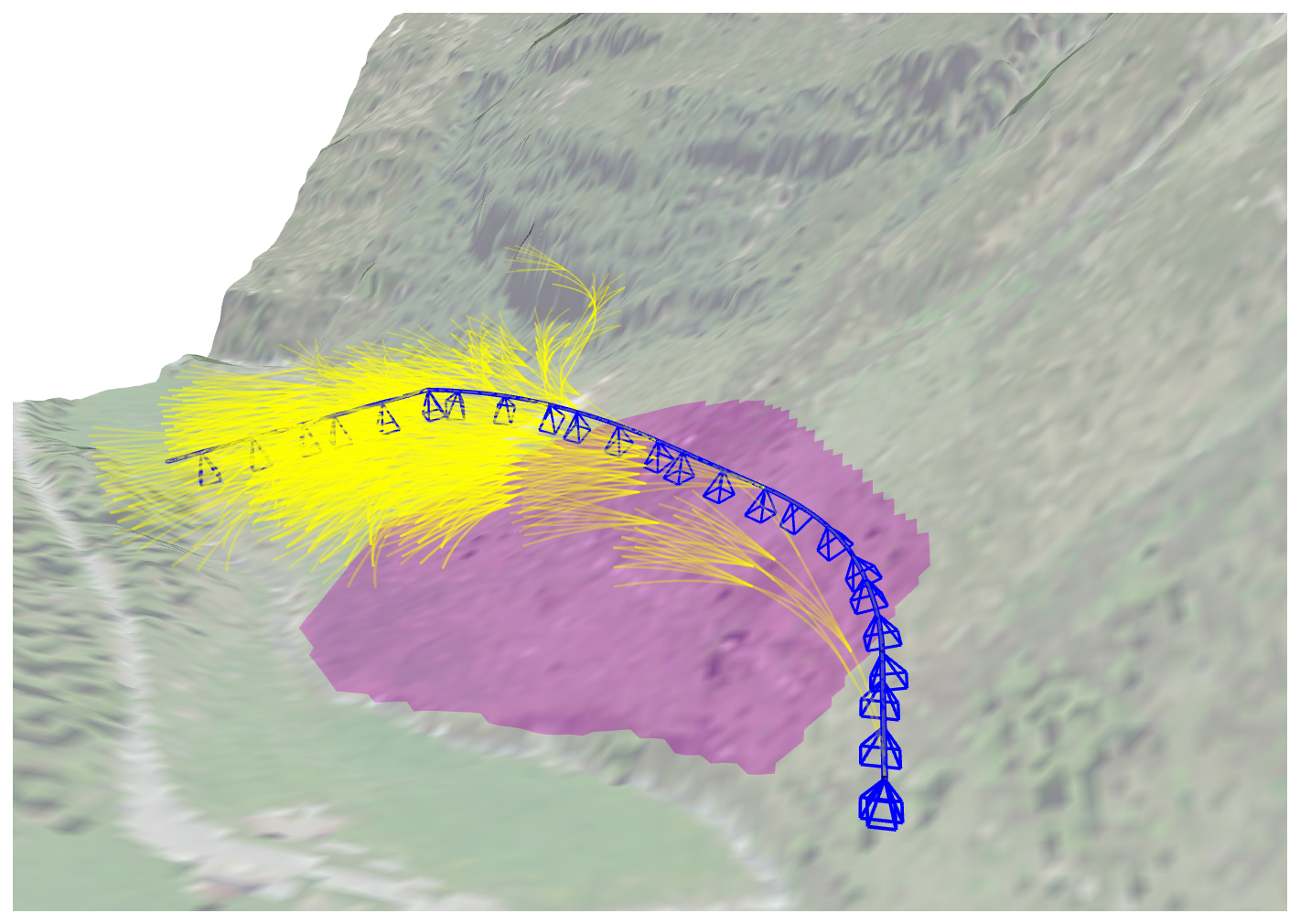
Figure 8 Visualization of the active planner mapping an ROI marked as a magenta overlay. The motion tree generated by monte-carlo tree search (MCTS) is highlighted in yellow. The best maneuver is highlighted as, with the expected viewpoints visualized as view frustums. Source of DEM: swisstopo (1998a). Source of orthoimage: swisstopo (1998b).

The proposed active mapping system does not require explicit waypoint planning like conventional coverage approaches do. The active mapping is formulated as a sequential decision-making problem, where the objective is to find a safe sequence of feasible maneuvers that maximizes the quality of the photogrammetric reconstruction. We use a view utility metric based on Fisher information proposed in Lim et al. (2023b), to estimate the usefulness of views taken in a particular motion sequence for photogrammetry. By estimating the uncertainty of a photogrammetric reconstruction using camera network geometry, the usability of a viewpoint can be estimated without running reconstruction in the loop. Note that this method relies on the expected prior geometry, based on the DEM. In avalanche terrain, this could introduce errors due to accumulated snow or vegetation that may not be part of the DEM. Moreover, this can result in occlusions. While having a wrong prior would result in wrong uncertainty estimates, we empirically show that using a DEM on avalanche terrain is a sufficient proxy for view planning. However, future research could include online reconstruction techniques to update the uncertainty estimate of the camera network geometry.

In order to solely consider feasible maneuvers (i.e. actions that can be achieved by the aircraft), we discretize the maneuvers using a motion primitive tree. This involves creating a discrete set of maneuvers and forward-propagating each action from the vehicle's current state with a motion model. In this work, we consider constant curvature maneuvers, that can be defined as a curvature value κ∈K and flight path angle γ∈Γ, where K, Γ are the set of feasible curvatures and flight path angles, respectively. We consider 9 maneuvers in the maneuver set $\mathcal{A}=K\times \mathrm{\Gamma }$ where $K=\mathit{\{}-{\mathit{\kappa }}_{max},\mathrm{0},{\mathit{\kappa }}_{max}\mathit{\}}$, $\mathrm{\Gamma }=\mathit{\{}-{\mathit{\gamma }}_{max},\mathrm{0},{\mathit{\gamma }}_{max}\mathit{\}}$. Each maneuver is forward propagated with a fixed time duration Δt=3 s using the Dubins Airplane model, where the state space is defined as $\mathbf{x}=(x,y,z,\mathit{\theta })$ (shown in Eq. 1).

$$\begin{array}{}\text{(1)}& \dot{\mathit{x}}={\displaystyle \frac{\partial \mathit{x}}{\partial t}}=\left(\begin{array}{c}\dot{x}\\ \dot{y}\\ \dot{z}\\ \dot{\mathit{\theta }}\end{array}\right)=\left(\begin{array}{c}V\cos \left(\mathit{\gamma }\right)\cos \left(\mathit{\theta }\right)\\ V\cos \left(\mathit{\gamma }\right)\sin \left(\mathit{\theta }\right)\\ V\sin \left(\mathit{\gamma }\right)\\ \mathit{\kappa }\cos \left(\mathit{\gamma }\right)\end{array}\right)\mathrm{s}.\mathrm{t}.\mathit{\gamma }\in \mathrm{\Gamma },\mathit{\kappa }\in K\end{array}$$

To reduce the search space, actions that violate the constraints are pruned (not considered). Additionally, to prevent the vehicle from entering an ICS, a motion primitive is considered invalid if none of the children is a valid motion primitive. In this work, we focus on optimizing 10 sequences of motion primitives, amounting to planning for 30 s of receding horizon planning. This results in a total of 9¹⁰ possible different maneuver sequences to evaluate every 3 s.

Due to the high number of maneuvers that need to be evaluated, it is not feasible to exhaustively search through all the possible maneuver combinations. Therefore, we use MCTS, an anytime approximate graph search algorithm (Browne et al., 2012), to evaluate and identify promising motions from the tree in real-time. Figure 8 shows a snapshot of the motion tree and the resulting maneuver planned. The maneuvers are planned in a rolling window fashion, where after each maneuver is executed, the next best maneuver of a horizon of 10 maneuvers is planned. The utility metric is computed through viewpoints along the path, where it is assumed that the camera image is triggered at 1 Hz, which ensures that there is sufficient overlap between the consecutive images.

3.4 Operations

A 3D graphical user interface (Fig. 9) is used by the operator to interact with the vehicle. The operator sends commands such as target position, or vehicle states, and the autonomous planner ensures that the vehicle can be operated safely. The user interface consists of a planning panel, interactive marker, and 3D visualization of the vehicle information. The planning panel contains clickable buttons, which the operator can use to control the state of the vehicle or engage and disengage the autonomous planner. Depending on the current state, the states that cannot be set are grayed out according to the state machine (Fig. 6).

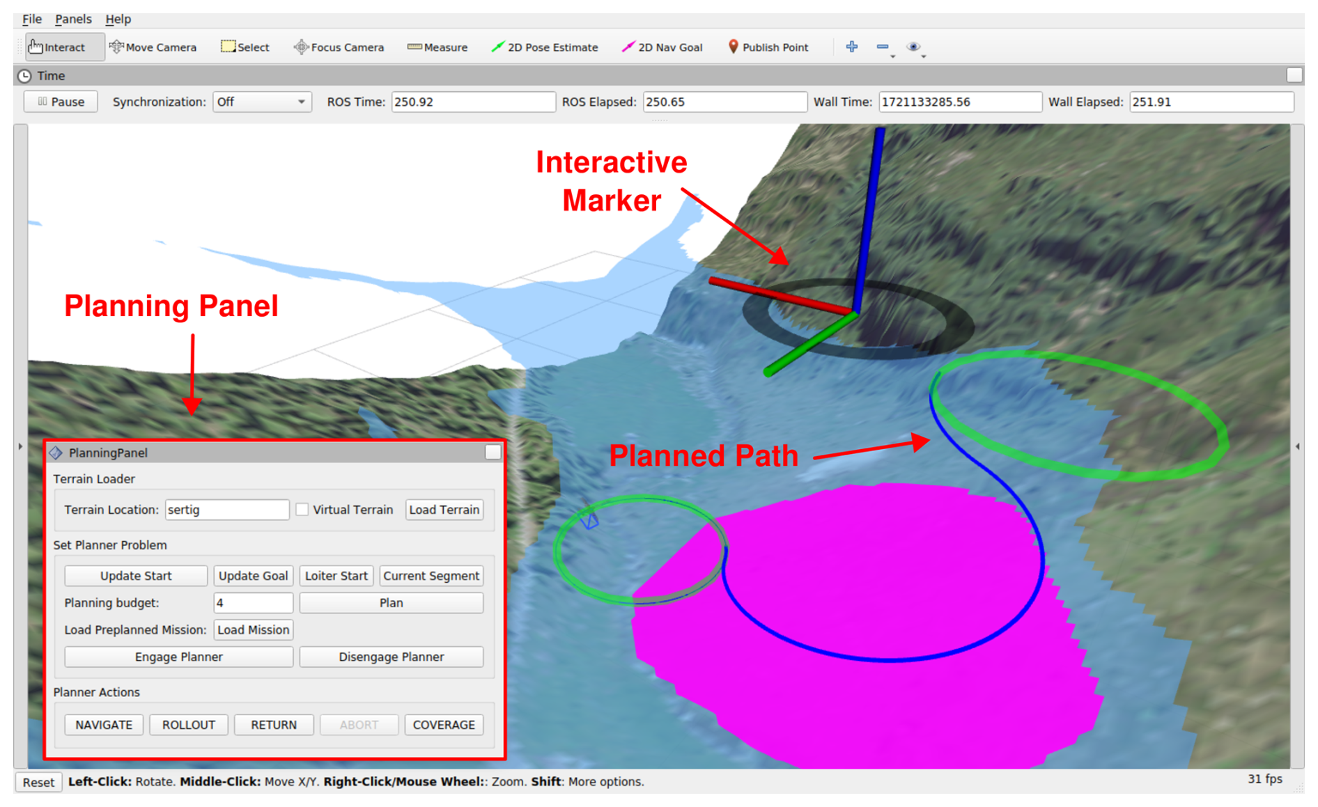
Figure 9 Operator interface for controlling the vehicle: the Planning panel is used for commanding actions, such as mode switches, or engagement of the autonomous planner. The interactive marker is used as a cursor to specify goal positions in the map. The planned path is visualized, for better situational awareness to the operator. Source of DEM: swisstopo (1998a). Source of orthoimage: swisstopo (1998b).

The interactive marker serves as a cursor, where the operator can dynamically choose the target position on where the vehicle should navigate. For example, if the vehicle is in the Hold state, the operator can define the goal position through the interactive marker. When the operator switches to the Navigate state, the autonomous planner finds the shortest path from the current loiter to the target loiter path and the vehicle follows it.

Information on the vehicle state is visualized in the 3D visualization. The information includes vehicle information such as speed and location and the reference path that the vehicle is following. Additionally, the DEM and ROI are visualized to provide better situational awareness to the operator. The DEM and ROI is loaded onto the vehicle before the flight.

4 Field Demonstration

We validate the system in a real-world field test, where the vehicle is deployed in alpine terrain to map an avalanche deposit in Davos, Switzerland (Fig. 10). We demonstrate a case where the vehicle is trying to map a single ROI when the vehicle has arrived at one of the loiter points. While this experiment does not include the route optimization and mapping of multiple ROI, the crucial functionalities such as safe navigation and path following are demonstrated through the single ROI mapping experiment.

Figure 10 Flight testing location placed in the Flüela Valley in Davos, Switzerland. (a) 3D visualization of terrain and ROI used for mapping. (b) Field test location and ROI visualized in map. Source of DEM: swisstopo (1998a). Source of orthoimage: swisstopo (1998b).

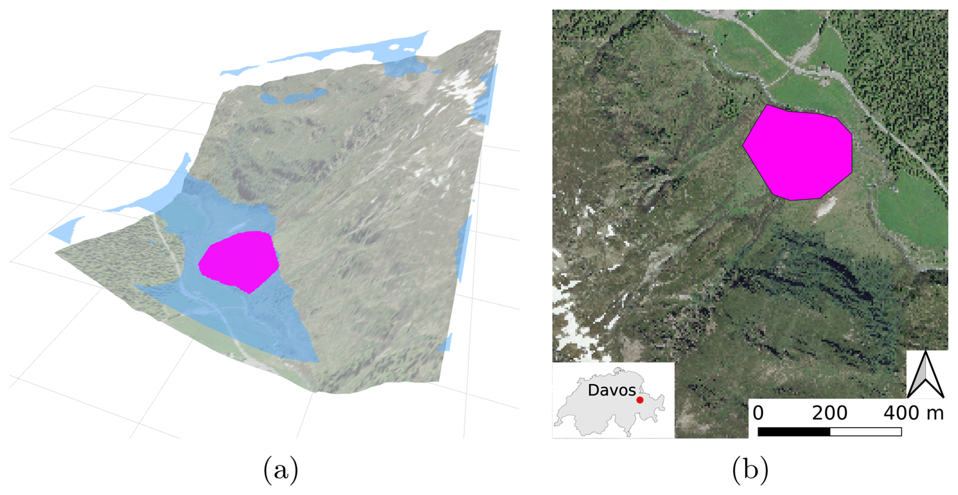
The experiments were conducted on the 25 April 2024, in the Flüela Valley in Davos, Switzerland. The ROI was defined around an avalanche deposit, where the extent of the ROI was outlined by hand where the the avalanche was observed. The ROI, however, only contained part of the avalanche due to operational constraints, such as visibility of the safety pilot. The weather was sunny, and the observed wind speeds were on average 2.8 m s⁻¹ with a maximum of 3.6 m s⁻¹. The snow had relatively little texture as there was fresh snow from a snowfall event the day prior to the field test.

4.1 Setup

The goal of the field test is to demonstrate a full mapping mission, where the sUAS autonomously navigates through steep alpine environments safely, is capable of autonomously mapping an ROI, and finally returning to the start position. We focus on two aspects of the field test: first, we evaluate whether the vehicle stays within the altitude constraints throughout the mission, which is defined by 50 m to 120 m a.g.l. This would show that the vehicle can maintain a safe distance to the terrain (at 50 m) and comply with the regulation by staying within 120 m a.g.l. despite the constrained maneuverability of the vehicle. The DEM around the mission area is loaded onto the vehicle, which is used for navigation.

Second, we evaluate the effectiveness of the active mapping approach and compare it with a baseline coverage planning approach. An ROI is defined prior to the mission through a polygon, which is used for creating a smaller DEM that is used by the active mapping (Fig. 10a).

The coverage planning method is based on a conventional boustrophedon decomposition (Choset and Pignon, 1998), generating sweep patterns from a specified sweep direction. The sweep spacing was set as 67.4 m, which corresponds to an overlap percentage of 70 %. This is compatible with the industry standard of 60 % to 80 % overlap between sweeps. The trigger rate was set to 1 Hz, in order to keep it comparable with the active mapping approach. However, conventional coverage approaches (Bähnemann et al., 2021; Mier et al., 2023) can not satisfy the distance-to-terrain constraint or consider the kinematic constraints of the vehicle. Therefore, the sweep patterns are adjusted, such that the altitude of the endpoints is 100 m above the terrain. After the sweep patterns are generated, the path to traverse between the sweep patterns is planned by formulating a path planner as done in Lim et al. (2024a). Note that a cross-grid coverage pattern was not considered, as the steep terrain prohibits the vehicle from following sweep patterns that are orthogonal to the main sweep patterns.

As the active mapping method does not have an explicit termination criterion, for evaluation the operator commands an Abort once the duration of the mapping state is longer than the duration of the coverage survey. In the mapping state, the vehicle takes images of the target region, which is post-processed for reconstruction after the flight. We compare the reconstruction quality and the time to get equal reconstruction results. Comparison with other sensing modalities was not included in the campaign, as the vehicle is not capable of carrying other sensing modalities such as LiDAR or ground penetrating radar (GPR).

4.2 Safe Navigation

The 3D visualization of the planned path during field tests shows that the vehicle was able to safely approach the ROI, autonomously map the environment, and safely return to the original loiter position (Fig. 11a). During the field test, the vehicle went through all flight states – Hold, Navigate, Mapping, Abort, Return – validating safe operation and transition between different modes. We evaluate whether the planner was able to plan a safe path that stayed within the constraints, defined as staying between the maximum (120 m) and minimum (50 m) distance from the terrain. The reference point is calculated as the closest point on the planned path from the vehicle and, not the vehicle position. The evolution of the reference point during the flight test is displayed with the terrain elevation directly below the reference position (Fig. 12).

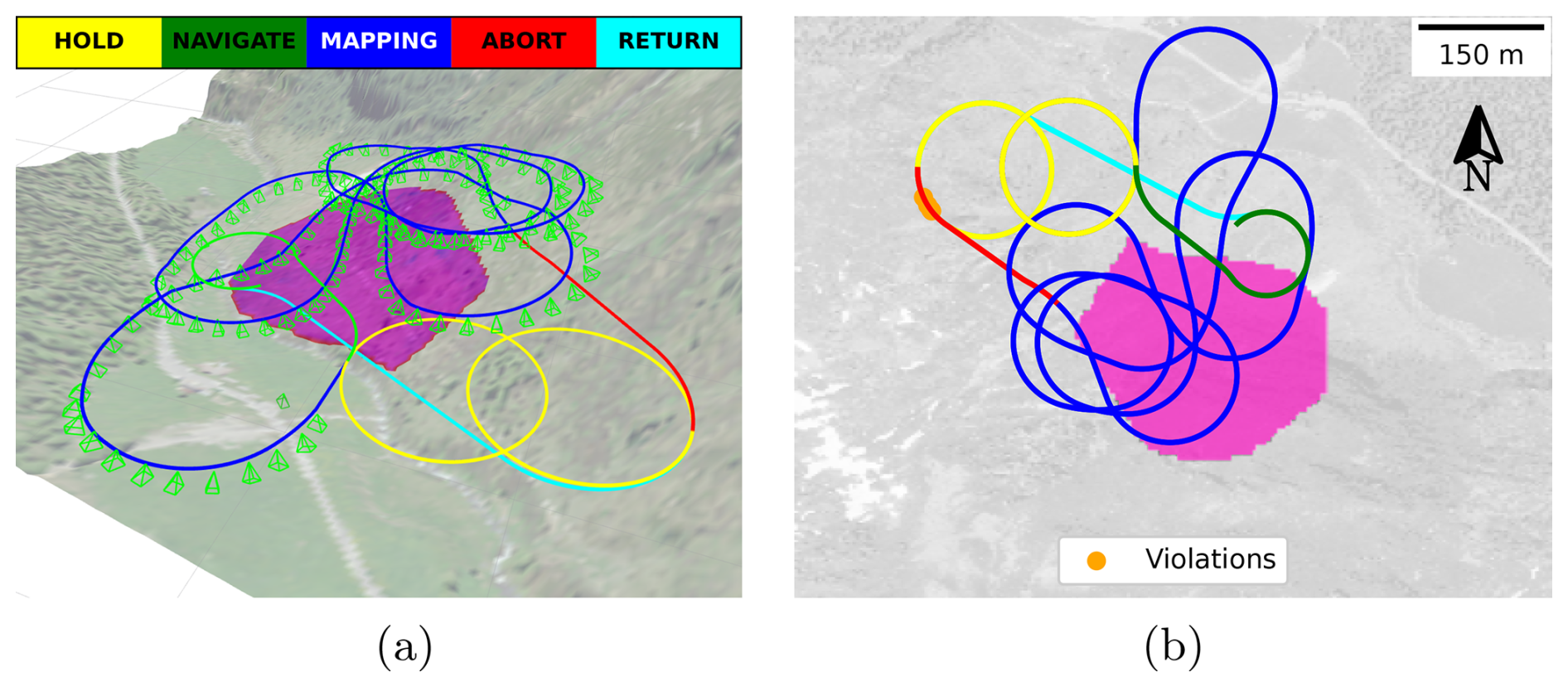
Figure 11 (a) 3D visualization of active mapping path and viewpoints acquired during field tests visualized with the interface from the autonomous planner. The reference throughout the mission is color-coded for each of the states. The viewpoints acquired during the mapping state are visualized as green view fustrums. The magenta region shows the region of interest. (b) 2D visualization of active mapping path and projected on the map. Orange circles marks a violation of the distance constraints. Source of DEM: swisstopo (1998a). Source of orthoimage: swisstopo (1998b).

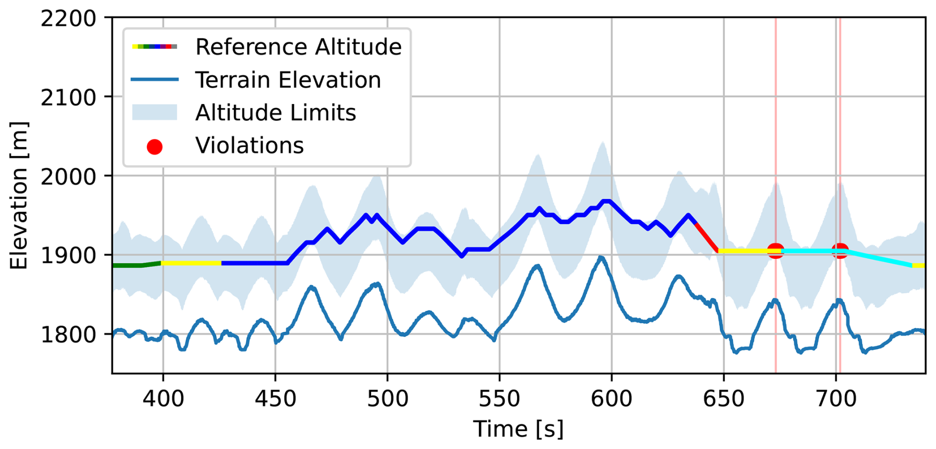
Figure 12 Altitude of the reference position, colored with the flight mode. The terrain altitude below the reference position is plotted in solid blue. The flyable space that satisfies distance-to-terrain constraints is visualized as a blue overlay. Violations of the reference is visualized as red.

Throughout the flight, the reference stayed within 50 m to 120 m most of the time, with two separate violations of the minimum distance constraints (Fig. 12). It can be seen that the terrain elevation change can be significantly steeper than what the vehicle can achieve, highlighting the need for a global path-planning approach to ensure safety. Especially, the steep regions of the state space only permit a narrow corridor, where the reference can be as close as 1.73 m from the maximum permitted elevation. The two violations in 672.69 and 701.42 s, with a duration of 0.90 and 0.87 s occur in a similar region of the loiter circle after the abort of the active mapping (Fig. 11b). The cause of the violation is the discretization effects of the elevation map and how the circle is iterated over the grid cells. As the map resolution is 5 m, the discretization of calculating the maximum and minimum distance surface causes some of the states to violate the terrain constraints in steep regions.

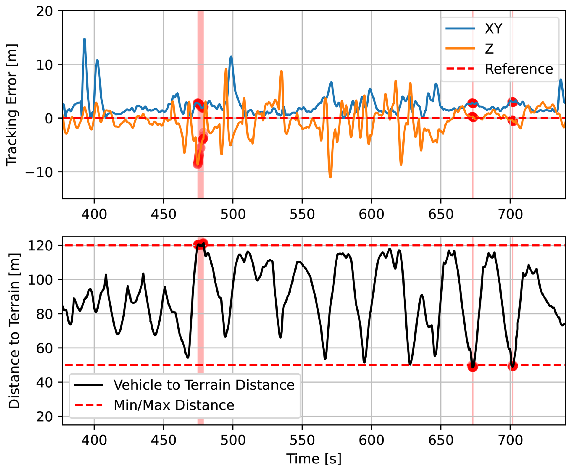
Figure 13 (Top) Tracking error in X, Y, Z for the vehicle to the planned reference. The large tracking errors come from the discontinuous changes in curvature and flight path angle of the reference path. Violations of constraints are marked as red circles. (Bottom) Vehicle Distance to Terrain. The vehicle briefly violated the altitude constraints three times during the flight test (each < 1 s).

While the reference, which is on the planned path, mostly satisfies the distance constraints, the vehicle is not perfectly tracking the reference. Therefore, we evaluate the tracking performance of the vehicle during the mission. Specifically, we evaluate whether the vehicle stayed within the constraints, by calculating the distance of the measured vehicle positions from the terrain (Fig. 13). The maximum tracking error is 14.84 m and root mean square error (RMSE) is 3.99 m. While the vehicle stays within the constraints most of the time, there were three violations where the vehicle did not stay within the distance limits. Out of the three events, the latter two violations happened due to the references violating the constraints, where the violation happened at 701.25 s for 0.97 s where it violated the constraints of 0.949 m and at 672.49 s for 1.20 s where it violated the constraints by 1.39 m. In these two violations, it can be seen that the violations happen even if the tracking errors are small, as the reference have violated the constraints. The first event violated the maximum constraint, at 474.57 s where the altitude exceeded 1.4 m for 4.4 s. The cause of this violation can be attributed to the large tracking errors from the reference point. The large tracking errors are most significant when there are large discontinuous curvature changes or flight path angles in the path. These discontinuities are inherent in the Dubins airplane path representation, which is dynamically infeasible for the vehicle. Given that the regulation only enforces the maximum distance constraints, there was one event of violation of the regulations throughout the whole flight, which was caused by large tracking errors.

4.3 Active Mapping

We evaluate the active mapping approach by demonstrating that it is capable of capturing images that create a complete reconstruction of the ROI. Then we compare the efficiency of the active mapping approach to a conventional coverage planning approach, where we compare the time it took to map the ROI and the reconstruction quality of the image dataset acquired from the flight. Since the active mapping planner does not have an explicit termination time, it is run for the same duration as needed for the coverage planning based mission. This allows for comparison by the duration of the mapping mission from the time when the first image was taken. The active mapping mission resulted in 167 images, where the camera was triggered at a fixed rate at 1 Hz (Fig. 11). The path from the coverage mapping shows that the vehicle follows a sequence of 5 straight sweeps, resulting in 47 images (Fig. 14). The difference in image count is, for one, because the coverage plan is fixed based on the geometry of the ROI, while the active mapping approach will continue indefinitely to further minimize the uncertainty of the mapping result. In order to have a fair comparison with the methods, the coverage mapping approach also had a fixed rate of camera triggering at 1 Hz, albeit only during the traversal of the straight sweep lines.

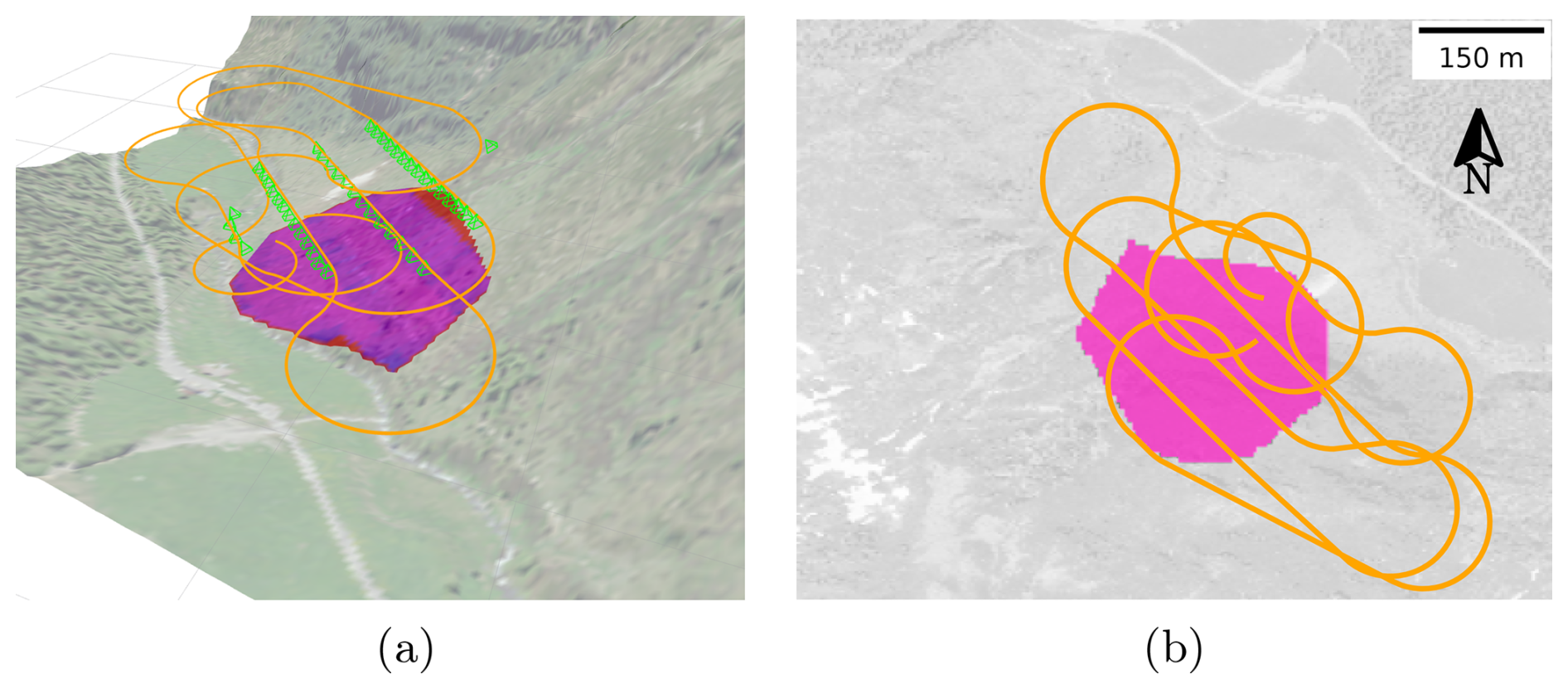
Figure 14 (a) 3D visualization of coverage mapping path during the flight tests, where the flight path is displayed in orange and view frustums are visualized in green. The target region of interest is shown in magenta. (b) 2D visualization of coverage mapping path projected onto the map. The coverage path starts at the highest sweep, and then sequentially flies through the coverage sweep patterns. Source of DEM: (swisstopo, 1998a). Source of orthoimage: (swisstopo, 1998b).

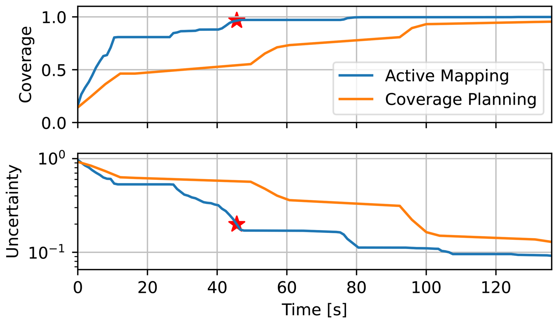
Figure 15 (Top) Coverage comparison of active mapping and coverage mapping. (Bottom) Expected uncertainty comparison with active mapping and coverage mapping. The point in time with 67 images taken is marked with a red star (★).

We look at two metrics prior to the reconstruction to evaluate the active mapping approach. The first is coverage, in which we consider as the portions of cells in the elevation map that was observed from more than two viewpoints. This is because two viewpoints are necessary conditions in which a reconstruction can be created at that position. The second metric is the fisher-information-based average expected uncertainty (Lim et al., 2023b), which quantifies the epistemic uncertainty expected from the photogrammetric reconstruction.

The active mapping approach achieves a significantly higher coverage within less time, where active mapping takes 44.5 s compared to the coverage planning approach that took 131.2 s to achieve 95 % coverage (Fig. 15). This is due to the oblique viewpoints of the active mapping approach, which maneuvers the aircraft at high roll angles. This results in a wider field of view in contrast to coverage planning approaches, which always assume a nadir viewpoint. Additionally, coverage planning was only able to achieve coverage at 95 %, while active mapping fully covered the ROI.

The expected uncertainty decreases significantly faster for the active mapping method than for coverage planning. The final uncertainty which the coverage planning took 135.73 s to achieve, took active mapping 79.42 s, which the time is reduced by 58 % by using the active mapping approach. Additionally, the final expected uncertainty at the end of the mission is also 57 % lower for the active mapping method (0.074 vs 0.129; Fig. 15). This is because the maneuvers selected by the active mapping planner are optimized to reduce the uncertainty, in contrast to coverage planning, which simply follows a path to geometrically achieve coverage. Therefore, coverage planning does not achieve full coverage until all the sweep patterns are flown. Additionally, the active mapping planner can continue to acquire viewpoints which reduce uncertainty even after the scene has been fully covered. Another reason for the coverage planner being slow is because of the images are only acquired during the straight sweeps and not during the turns between them. This results in steps, where during turns the improvement of coverage and uncertainty is stalled.

We analyze the difference of the image dataset by looking at how the surface of the ROI is being mapped. We look at each point of the surface, the number of views that are visible, and the expected uncertainty (Fig. 16). It can be seen that the number of views visible on the surface is much higher for the active mapping approach. This can be explained with the oblique viewpoints covering large areas of the surface with a single viewpoint. For coverage planning, parts of the ROI have no views which was caused by a mistrigger of the camera. While similar mistriggers happened during active mapping, the planner was able to compensate for the missed image due to the receding horizon planning to repair the reconstruction.

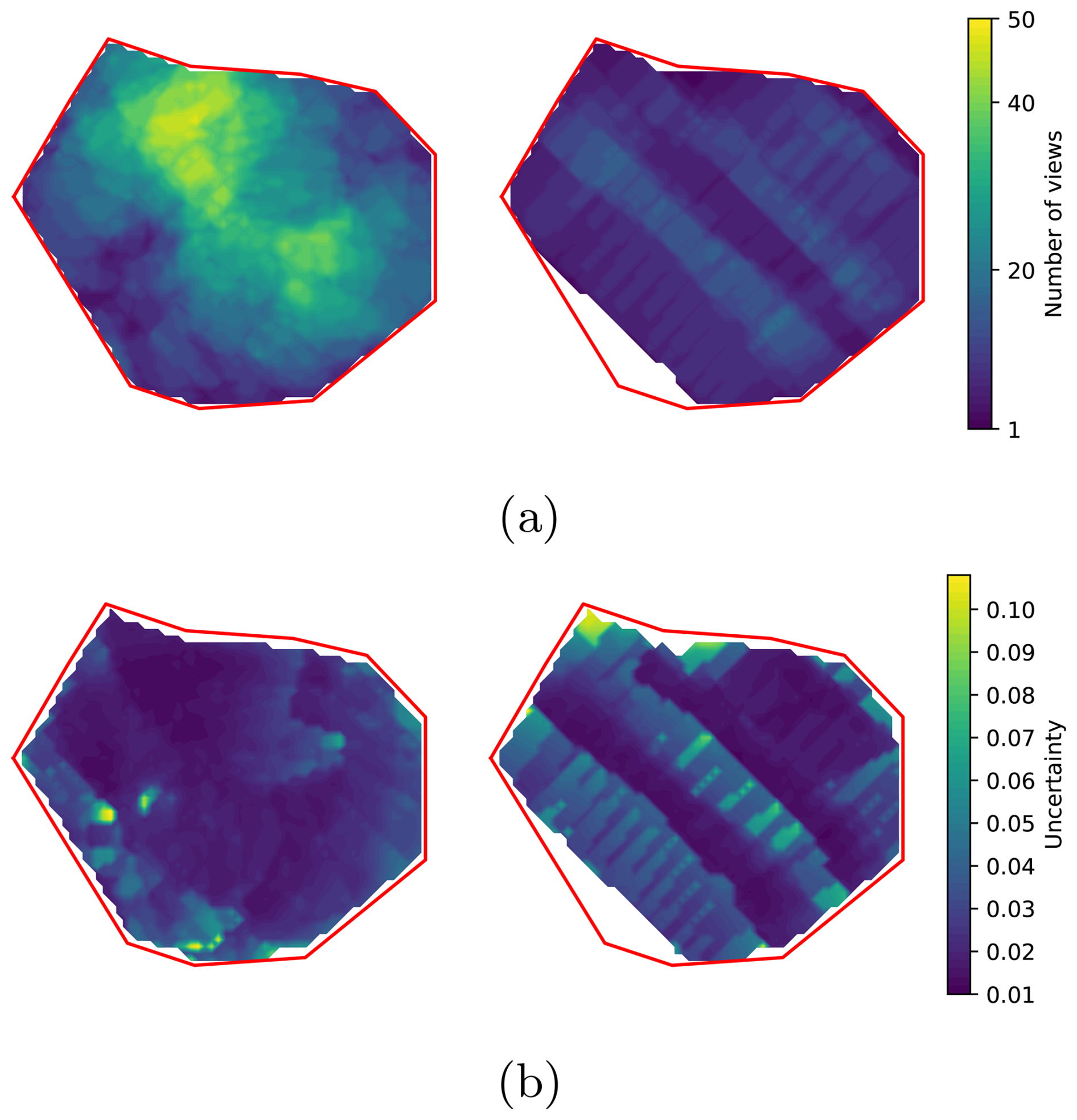
Figure 16 Comparison of the (a) number of views, number of overlapping views, and (b) expected uncertainty and expected uncertainty between active mapping and coverage mapping after flight test (Left: Active Mapping, Right: Coverage Mapping). The ROI outline is marked as a red line. Regions with no color inside the ROI are regions on the surface that have zero views visible.

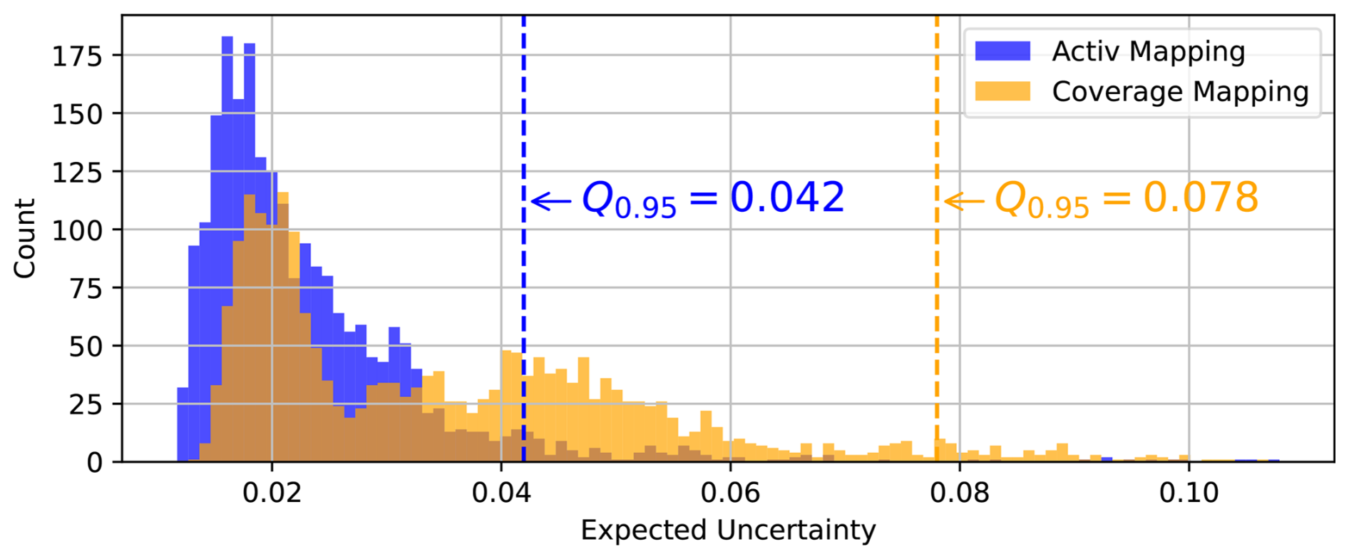
Figure 17 Distribution of uncertainty across the mapped surface inside the ROI. 95 quantile of expected uncertainty with active mapping is 0.042, significantly lower compared to coverage mapping of 0.078.

The expected uncertainty on the surface, is qualitatively more evenly distributed with active mapping. Coverage mapping shows different levels of uncertainty along the flight lines and image overlaps (Fig. 16b). Histogram analysis shows that, under the active mapping approach, the uncertainty distribution is shifted toward lower values (Fig. 17). Moreover, the 95 quantile of expected uncertainty for active mapping is 0.042, in contrast to the value of coverage mapping of 0.078. This shows that the 95 quantile is reduced by 47 %, demonstrating that the active mapping approach results in a significantly lower expected uncertainty value over the surface. Comparing the visibility count and the expected uncertainty in coverage planning, it can be seen that the high-uncertainty regions do not necessarily correlate with regions of low visibility count. This is due to the steep slope of the target terrain, where the high uncertainty regions are downslope regions where the GSD gets worse during the sweep of the survey.

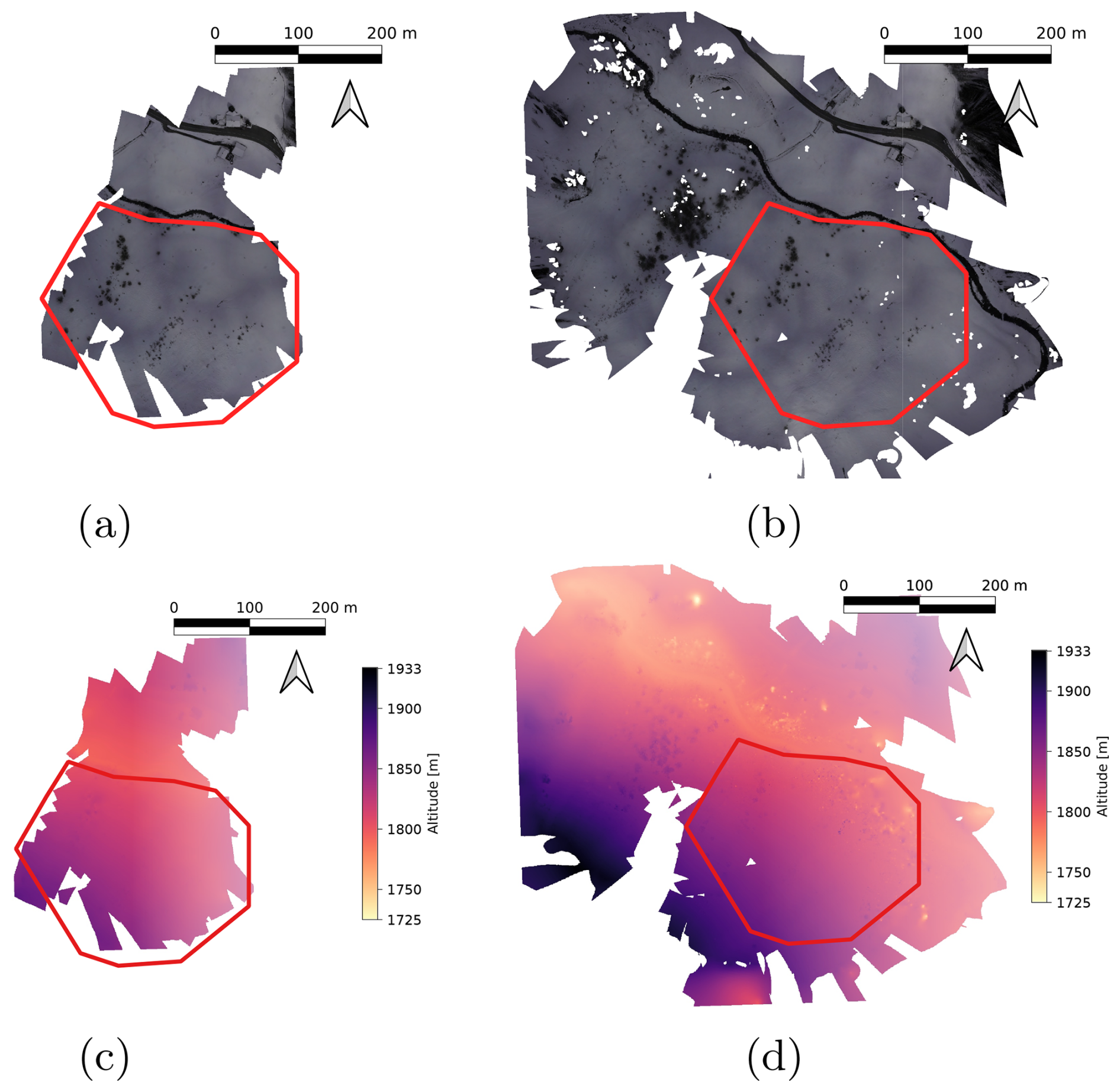
Figure 18 Reconstruction of orthomosaic and elevation reconstruction using active mapping using partial dataset (67 images) and full dataset (167 images). The red polygon represents the ROI. (a) Orthomosaic reconstruction using partial dataset of 67 images. (b) Orthomosaic reconstruction of final result with 167 images. (c) Elevation reconstruction using partial dataset of 67 images. (d) Elevation reconstruction of final result with 167 images. The orthomosaic generated from active mapping covers a significantly larger area than the ROI, which comes from images that were taken while the vehicle was outside of the ROI as the camera is triggered at a fixed rate.

We compare the reconstruction quality of the image dataset that is acquired during the mission. Figure 18 shows a qualitative comparison of the orthomosaic and elevation reconstruction using the commercial photogrammetry software Agisoft Metashape (Agisoft, 2024a, b). We refer the readers to the Supplement for the processing report of the reconstruction. The reconstruction from the active mapping method shows that it successfully covers the ROI (Fig. 18b). The orthomosaic covers a significantly larger area than the ROI, which comes from images that were taken while the vehicle was outside of the ROI as the camera is triggered at a fixed rate. For comparison, we show a reconstruction of the active mapping method in the middle of the survey after 67 images (Fig. 18a). This corresponds to t=45.63 s (Marked in Fig. 15). It can be seen that a significant part of the ROI is already covered while a fraction of the time has been spent in mapping. This is an expected result, as we have seen in the steep increase in coverage and expected uncertainty. Also, from the elevation, it can be seen that the reconstruction from the partial dataset lacks some details around the vegetation. This shows that active mapping improves the reconstruction quality, as it continues to gather data.

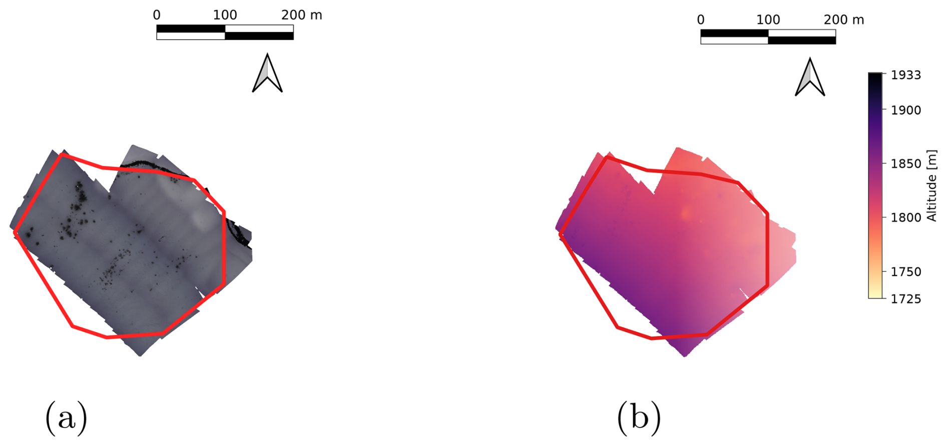
Figure 19 Qualitative comparison of (a) orthomosaic and (b) elevation reconstruction with data acquired by coverage mapping (47 images). The red polygon represents the ROI.

Similarly, the reconstruction of orthomosaic and elevation from image acquired from coverage mapping is compared. The reconstruction shows a much more conservative reconstruction around the ROI. Part of the reconstruction is missing, due to both a mis-triggering of the camera in the beginning, and a failed registration at the end of the survey. This shows that while image data of coverage methods can result in a good reconstruction, it is much more sensitive to issues such as camera triggering or image registration working. Additionally, the orthomosaic results show much less coverage compared to what was predicted with expected uncertainty. Since the surface is always viewed from the same direction, the failed reconstruction on the northern corner of the ROI is due to the viewpoints being more susceptible to bad feature matches due to the low texture of the snow Fig. 18.

Figure 20 Absolute difference of reconstructed elevation between active mapping (Fig. 18d) and coverage mapping (Fig. 19b).

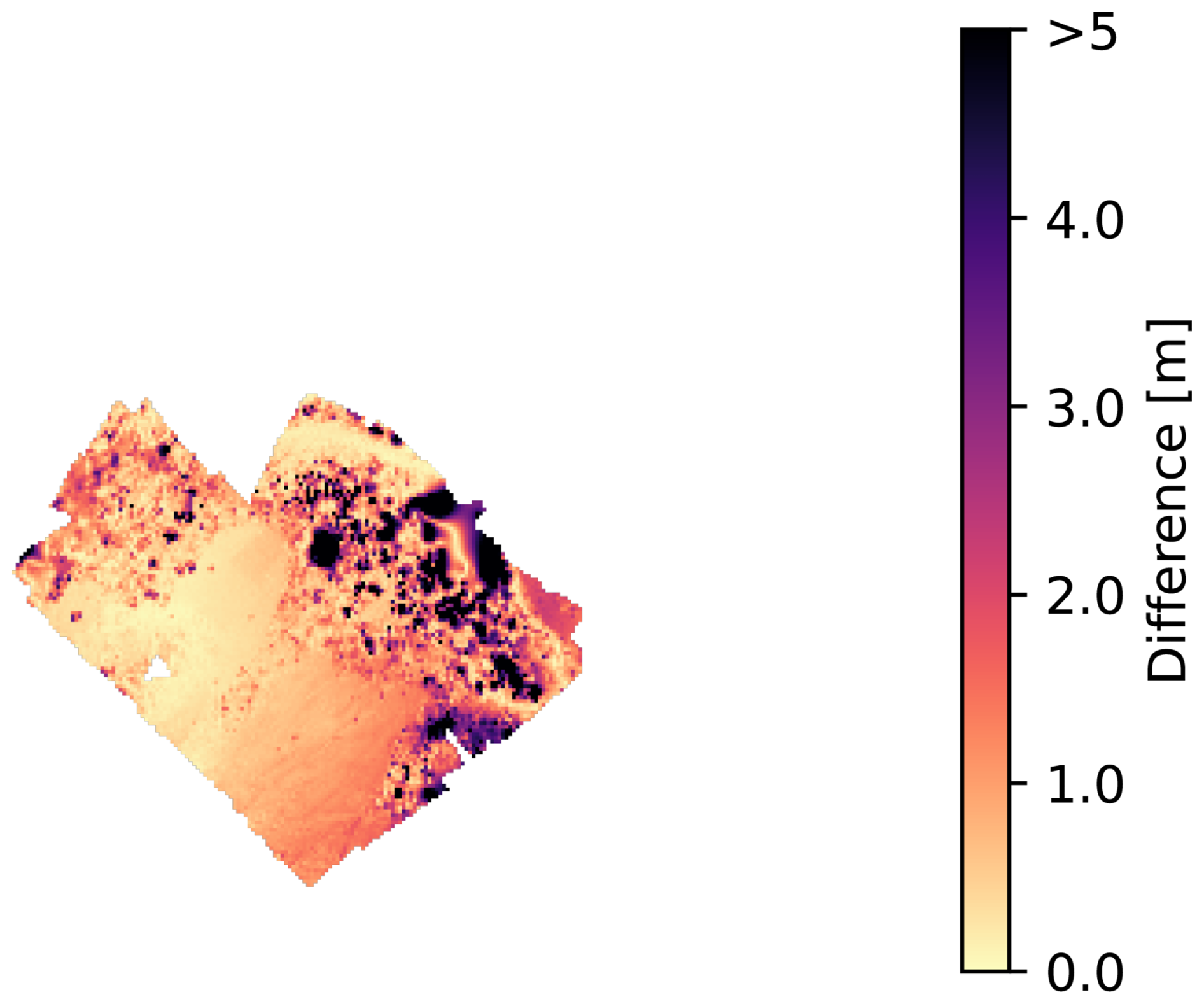
By comparing the difference between two elevation maps, we can see how consistent the reconstruction is (Fig. 20. The root mean squared error of the two maps is 2.71 m. Note that qualitatively the error does not match how the expected uncertainty is distributed in Fig. 16b. This is because the proposed approach does not consider appearance or texture of the surface, which can have a large impact on the quality of reconstruction. More discussion regarding this problem can be found in Sect. 5.1.

5 Discussions

The integration of a finite state machine provides a simple abstraction to the complexity of operating a VTOL vehicle. For navigation-related tasks such as Navigate, Abort, Return the operator only needs to specify a target objective such as a 2D goal position for the planner to dynamically discover a a safe path. This greatly simplifies the operational complexity, in which every mission needs to be carefully designed to operate a fixed-wing vehicle. Most conventional fixed-wing vehicle missions are described as a sequence of straight lines, which makes missions close to the terrain almost impossible in mountainous terrain. Such capability is essential especially for long-endurance vehicles operating beyond visual line of sight, as missions can include multiple objectives and events, which may be impractical to pre-plan every scenario.

In this work, state transitions were commanded by the operator. This was to explicitly demonstrate the dynamic nature of the capabilities of the vehicle, and ensure to make it easier to monitor the system during the field tests. However, the state transitions can be automated for more autonomous operations. For example, a mission with a sequence of target positions and state transitions can be defined prior to the mission, where the vehicle can autonomously navigate to the target position close to the ROI, and map the environment. One needs to simply define how to determine when a task is done, such that the state can be transitioned to the next state.

5.1 Benefits and Limitations on Active Aerial Photogrammetry

To the author's knowledge, this is the first demonstration of an active mapping method deployed on a fixed-wing vehicle. The reason active mapping is efficient is due to the use of dynamic maneuvers and oblique viewpoints to take more informative viewpoints, without compromising the quality of the reconstruction.

While the field tests demonstrated that the active mapping approach can be more efficient than coverage planning approaches, field tests have shown that the reconstructability metric does not always ensure good reconstructions. This is due to the fact that the expected uncertainty is computed only using the camera network geometry, assuming that a feature would exist to reconstruct the surface. While this may be a limitation of this approach, practical challenges can arise for processing image data in real time, especially for high-resolution cameras used for photogrammetry. For example, a single image taken by the photogrammetry camera was 9504×6336, and 18.5 MB in size. Therefore, the proposed approach enables view planning with information that can be easily accessible on the system during data acquisition. However, not considering appearance may be limiting in challenging scenes such as mapping homogeneous snow surfaces. For future works, methods considering appearance in addition to the camera network geometry (Liu et al., 2022; Kim and Eustice, 2013) could be useful for solving this problem.

Lastly, the active view planning approach plans maneuvers in a receding horizon manner. This is in contrast to the approach used for the safe navigation planner, as the terminal maneuver is evaluated for safety. As the horizon of the active mapping is relatively large (30 s), the probability of the vehicle heading into a dead end is low. Therefore, the maneuver generated by in the Mapping state is not guaranteed to be safe. Additionally, if the terminal state of the receding horizon path is constrained to stay within the terminal safe set (such as the valid loiter region), then the plan becomes too conservative and will not be able to enter steep terrain. Future work should address the problem of ensuring safety without the active mapping planner become too conservative.

5.2 Regulations

In this work, we have focused on complying with the EU regulations that have been effective in Switzerland since 2023 (European Commission, 2019). Under these regulations, operations of an aerial vehicle can be classified as visual line of sight (VLOS), extended visual line of sight (EVLOS) or beyond visual line of sight (BVLOS) depending on the distance the vehicle is operated from the operator. Under VLOS, the proposed system is classified in the open category, where no authorization is needed, as long as the vehicle is not flying over crowds and maintains altitude lower the 120 m a.g.l. Therefore, we have bounded the focus of our field experiments for mapping a single ROI to stay within VLOS. As the platform we have used in the experiments has a minimum turn radius of 80 m, maintaining such low AGL is challenging as the vehicle would not be able to make a full loiter in steep terrain. The brief violations of the constraints highlights how challenging compliance to the regulations can be, even with using an autonomous planner.

One of the major benefits of using fixed-wing vehicles comes from the long-range capability, and therefore BVLOS operations would allow access to remote regions. However, utilizing autonomous capabilities of the system would require improvements on the regulations. Current BVLOS operations require approval or a specific operation risk assessment (SORA), where a request for a single flight can be filed. This includes a predetermined flight route that needs to be filed. Therefore, these regulations make it hard to deploy the autonomous planner proposed in this work. We claim that autonomy makes the vehicle much safer to operate and enable the system to be more safe to intervene in case of an event such as avoiding air traffic. Additionally, while the BVLOS operations would potentially remove the tight constraints on AGL, staying at low altitudes could be considered as a lower risk for air-risk assessment procedures such as PDRA.

6 Conclusions and Outlook

In this paper, we have demonstrated a long-range autonomous fixed-wing sUAS capable of safely navigating and actively mapping a target region of interest in steep mountain terrain, also in winter. We have demonstrated how a route planning problem can be formulated as an orienteering problem, and how significant the efficiency of a mapping method can have an impact on the number of ROIs that can be visited within a single flight. Then we demonstrated on a real platform by integrating a safe path planner that safely navigates mountainous environments, considering the terrain and regulation constraints as well as the limited maneuverability of the fixed-wing vehicle. We also demonstrated an active mapping planner that iteratively plans the next maneuvers to optimize its viewpoints to maximize the information gathered.

The field demonstration has shown that the safe navigation planner is capable of guiding the vehicle to maintain a distance between the maximum and minimum distance constraints, which successfully operate the vehicle in a dynamic manner. The demonstration has also shown some shortcomings of the approach, including brief violations of the constraints due to the discretization of the elevation map and the large tracking errors of the vehicle. The field tests have also shown that the active mapping planner is capable of mapping an ROI with good coverage, while staying under the distance constraints.

Some of the shortcomings identified in this work can be addressed by direct improvement of the implementation. Discretization effects can be addressed in future work by taking a more conservative approach to inferring altitude bounds. However, it also points to a fundamental problem of using a discretized map representation for a continuous motion model of the system. Additionally, the tracking errors can be addressed by utilizing more advanced path-following controllers, such as predictive controllers.

The general approach is built on the access to prior knowledge of the terrain, described as the DEM. However, assuming the geometry of the surface as the DEM will not be accurate, due to snow cover, vegetation, or artificial structures. Additionally, the planner does not consider environmental effects, such as wind or very low temperatures, which may influence the performance of the vehicle significantly.

We envision that autonomous long-endurance fixed-wing aerial vehicles will become a powerful tool for gathering high-quality data for large-scale environment monitoring applications, not just for avalanche monitoring. This would allow for creating more robust, complete and reliable databases, which are essential for hazard mapping and mitigation measure planning. However, to efficiently apply UAS for these tasks, the regulations have to be met, which is currently a very difficult task, especially for autonomous systems. Future work would include improving robustness against environmental uncertainties such that the vehicle can operate in more adverse conditions that can occur in alpine environments and better predictions of reconstructability for photogrammetry.