Assessing financial risk to property portfolios from physical rainfall extremes

Physical climate risk from extreme rainfall is often poorly understood by financial investors, potentially extending to pension funds that manage assets of substantial societal importance. There is a growing need for investors to better understand these risks to ensure financial resilience in a changing climate. We present a transparent framework to estimate current and near-future financial risk from flood damage using rainfall hazard information from regional climate projections, river flood maps, and depth-damage functions. Synthetic portfolios are constructed from non-residential built-up surface data and country-specific property values, enabling calculation of Expected Annual Damage. Results show that this physical climate risk is already substantial and projected to rise consistently across Europe, with some regions experiencing particularly large increases. Portfolio composition strongly influences risk, with asset location and value at-risk inducing greater variability than climate model uncertainty. We also demonstrate how adaptation could significantly reduce Expected Annual Damage and deliver a strong financial return within a short time frame, reinforcing its role as a cost-effective strategy for managing climate-related risk. This approach offers a pragmatic and transparent method for quantifying an element of financial risk from extreme rainfall using openly available datasets. A key methodological limitation is the simplified statistical mapping between rainfall extremes and flood depth, which replaces a physically based hydrological modelling chain and is not explicitly validated against observations or hydrological simulations. As such, the results should be interpreted as indicative rather than decision-ready estimates of flood risk. Nonetheless, the findings highlight the urgent need for financial actors, such as asset managers, to integrate physical climate risk into decision-making to safeguard long-term financial resilience.

1 Introduction

Climate change is driving an increase in the frequency and severity of extreme weather events, with hazards such as heatwaves and extreme rainfall projected to become more common across Europe and globally (IPCC, 2023; Rajczak and Schär, 2017; Cardell et al., 2020). Advances in event attribution science now make it possible to assess the extent to which climate change has influenced specific extreme weather events by quantifying changes in their likelihood and intensity. For example, studies have shown that human-induced climate change increased the probability and severity of the widespread flooding that affected Western Europe in July 2021 (Tradowsky et al., 2023). Adverse impacts from extremes in Europe are projected to intensify, resulting in a range of socio-economic impacts, including increasing damage to infrastructure both inland and along coastal areas (e.g. Forzieri et al., 2018; IPCC, 2023; Deidda et al., 2026; Nawarat et al., 2026). An estimate of economic losses from weather and climate related extremes during 1980–2024 totalled EUR 822 billion across European Union member states, of which 47 % were associated with flooding (European Environment Agency, 2026). From the same estimate, EUR 208 billion (25 %) of the total losses for the 1980–2024 period occurred between 2021 and 2024 (European Environment Agency, 2026), highlighting that losses have intensified in recent years. Under future climate change scenarios, an example estimate of increased Expected Annual Damage to European properties is 5-fold under the Representative Concentration Pathway (RCP) 4.5 scenario and 7-fold under the RCP8.5 scenario by the end of the century (Devadas et al., 2025).

Financial markets are key catalysts for societal change across the wider economy, with pensions funds importantly holding huge cross-societal assets. To protect financial investments from the worsening intensity and frequency of weather extremes under climate change, pension fund risk assessments should consider physical risk from changing extremes now and in the future (Ranger et al., 2022). Bongiorno et al. (2022) demonstrate that a UK pension scheme faces significantly greater funding risks under three future climate pathways compared with a climate-uninformed baseline (where the baseline economic outlook does not consider climate change or related policy or technological change). During 2024, the Pensions Regulator in the UK revealed that quantitative risk analysis in climate disclosures is rare (The Pensions Regulator, 2024a), highlighting that many trustees achieve only minimum compliance with environmental social governance duties (The Pensions Regulator, 2024b) and, in 2025, suggested that pension schemes that cannot act to protect pensions from climate risk should quit the market (The Pensions Regulator, 2025).

Decision-making on climate risk can be hindered by a lack of transparent, robust, and decision-relevant tools for risk assessment within the financial sector. For example, Bingler and Colesanti Senni (2022) found that tools designed to assess transition risk (risk associated with the transition to a lower carbon economy) often lack transparency and provide limited communication of key assumptions and uncertainties. Similar challenges exist for physical climate risk assessment. Hain et al. (2022) identified substantial divergence in physical risk metrics reported by financial firms, raising questions about the consistency and reliability with which climate risks are incorporated into financial decision-making. More recently, a benchmarking exercise involving 13 climate risk vendors found considerable variation in both physical hazard estimates and projected damages for the same asset (Climate Financial Risk Forum, 2025). Likewise, Hoehn et al. (2025) observed substantial differences in risk estimates when providers were asked to assess a hypothetical pan-European real estate portfolio. Such inconsistencies can make it difficult for pension trustees, asset managers, and other financial decision-makers to confidently assess and manage climate-related risks. Effective physical climate risk management requires a strong understanding of climate science, modelling assumptions, and uncertainty. However, while climate service providers have legitimate reasons to protect their intellectual property, the methodologies underpinning commercial products are often not fully disclosed. As a result, users may struggle to evaluate whether model outputs are scientifically robust, appropriate for their decision context, or adequately reflect the range of plausible future climate outcomes.

User research has highlighted a demand within the financial sector for tailored guidance and decision-support resources to help users interpret and navigate complex climate information (Climate Financial Risk Forum, 2024). In this context, climate services research based on open datasets and openly published methodologies has the potential to improve transparency, support methodological development, and strengthen users' understanding of climate risk. Such approaches can empower financial institutions to conduct or commission tailored analyses and engage more effectively with climate service providers. Examples of openly accessible resources are beginning to emerge. These include the publicly funded, Excel-based Real Estate Asset Climate Testing (REACT) tool, which supports flood risk assessment for individual assets (de Model et al., 2023; van Veldhoven et al., 2024). Similarly, Wu et al. (2024) proposed open methodologies for flood hazard and vulnerability assessment that enable investors and asset owners to quantify climate risks across real estate portfolios in multiple locations globally.

Large pension portfolios may be spread across a nation, continent or globally. One way climate risk translates into financial risk is through potential asset damage caused by river flooding, driven by extreme rainfall in the surrounding catchment area over the preceding hours or days. Local flood risk to a particular asset would be best assessed by hydrological modelling which can model where the rain in a catchment ends up as flood water. However, due to technological and funding constraints, comprehensive local (high-resolution) hydrological models covering continental or global domains are not generally available as open data with quantified uncertainty information, nor are they guaranteed to be readily accessible for every location of interest through commercial providers. Given the geographically dispersed nature of many financial-sector portfolios, there is value in methods and tools that provide rapid and accessible estimates of extreme rainfall risk across large asset portfolios. While such approaches may be less robust than detailed local-scale assessments, they can support portfolio-wide risk screening where hydrological modelling outputs are unavailable. Such transparent methodologies can also be further improved and tailored to form commercial modelling products, particularly when including hydrological modelling inputs, or further developed in future research efforts. The open and transparent discussion around the methodological considerations and limitations can help support potential users of climate information in assessing their risk directly, or in discussions with commercial providers of tailored climate services.

Here we provide different scenarios of financial risk from a range of synthetic (invented) but plausible examples of portfolios using only public and freely available climate information and exposure and vulnerability data sources. Our method provides a framework for assessing financial risk through property damage from inland rainfall where other options are unavailable due to limited data access, resource, expertise or funding. In common with existing commercial flood risk products, there is no single “best” method for translating rainfall extremes into flood hazard, and different modelling choices can lead to substantially different risk estimates. Rather than eliminating this variability, the framework presented here seeks to make key assumptions explicit by providing a transparent and reproducible method. This transparency enables clearer comparison between alternative model configurations, such as different portfolio constructions, time periods, or modelling choices, supporting more informed interpretation of differences in risk estimates, in contrast to proprietary or black box methods where such differences may be difficult to diagnose.

While our method is transparent and pragmatic, a key component of this framework is a simplified statistical mapping between rainfall extremes and flood depth, which substitutes for a physically based hydrological modelling chain. This introduces substantial structural uncertainty, and therefore the resulting risk estimates are intended for illustrative and awareness-raising purposes rather than for decision-making at the individual asset level.

2 Data and Methods

This section provides an overview of the data and methodological steps underpinning our risk assessment framework.

2.1 Quantifying Risk

The aim of this study is to produce idealised flood risk information (maps, summary plots, statistics) that demonstrate both current and plausible future physical climate risks to property portfolios. Here, “idealised” refers to the use of simplified and synthetic representations of hazard, exposure and vulnerability, designed to isolate key drivers of risk and to illustrate the methodological framework, rather than to provide detailed, site-specific predictions. In this application, we do this for a region of North-West Europe covering the UK, Belgium, the Netherlands, Denmark and parts of France, Germany, the Czech Republic, Poland, Norway and Sweden (see Fig. 1), and covering two time-periods representative of the recent past and near-term future respectively. Note, however, that the approach could be applied to a different region and/or time period using the same or alternative data sources.

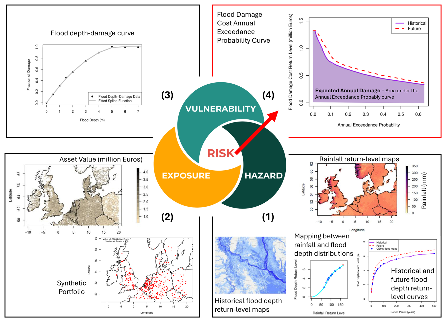
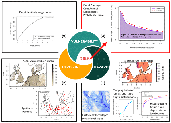
Figure 1 A schematic of the approach used to combine information about the hazard, exposure and vulnerability to estimate idealised flood risk (here Expected Annual Damage) for any given time period and at any given location. The stages of the approach are numbered: (1) Hazard: estimate the flood hazard by constructing a flood-depth return-level curve for each grid cell, based on rainfall return-level curves and a statistical mapping from rainfall extremes to flood depth (see Sect. 2.2). (2) Exposure: quantify the exposed asset value within each grid cell using built area and country-specific asset values per unit area (see Sect. 2.3). (3) Vulnerability: apply a depth-damage (vulnerability) function to the flood-depth return-level curve to map flood intensity to the fraction of asset damage, producing a damage-fraction return-level curve (see Sect. 2.4). (4) Risk: combine hazard, vulnerability and exposure to estimate flood damage costs and quantify risk by calculating the Expected Annual Damage as the numerical integral (area under the curve) of the flood damage cost annual exceedance probability curve (see Sect. 2.5).

To achieve this, we develop a methodology for estimating flood risk in any given time period and at any given location within the defined study region. This method involves combining three key components:

• Hazard: flood depth information representing the severity of inundation at a given location, for a given time period.

• Exposure: the estimated monetary value of assets at risk, derived from synthetic portfolio construction.

• Vulnerability: a depth-damage function that quantifies the proportion of asset value lost due to flood depth.

By combining these elements, we can produce spatially explicit and financially meaningful illustrative flood risk estimates.

The schematic in Fig. 1 provides an overview of this approach, described in more detail in the subsequent sections. Specifically, it illustrates: (1) how hazard information, extreme rainfall data and flood depth hazard maps, are combined to derive flood depth return-level curves (distributions) for any location and time period; (2) how exposure is represented by integrating asset values with synthetic portfolios, (3) how vulnerability is characterised through the relationship between flood depth and the fraction of damage to an asset, and (4) how these components are integrated to estimate the flood damage cost annual exceedance probability curve for the specified time period and location. The Expected Annual Damage (EAD), a key financial metric, is calculated as the area under this curve.

The following sections describe each part of this risk modelling change in more detail: hazard, exposure, vulnerability and how these are combined to estimate risk.

2.2 Hazard

To quantify flood hazard in a specific location and time period, we need to understand how frequently different flood depths occur at that location over the given time-frame. Ideally, risk estimation is based on a hazard event set, which represents a comprehensive collection of plausible hazard scenarios (e.g. floods, storms, earthquakes) along with their probabilities of occurrence. This approach allows for detailed modelling of losses across the full range of potential events, providing a robust estimate of risk metrics such as EAD. Currently, to our knowledge, no open-source flood depth hazard event sets exist for all return periods covering Europe in a consistent way for past and future climate length (20–30-year) periods, which constrains the application of this risk assessment approach. Although not an official flood hazard map, open-source river flood hazard data are available across Europe for nine return-levels (Baugh et al., 2026) alongside recently released satellite derived flood maps (Betterle and Salamon, 2026). Historical Analysis of Natural Hazards in Europe (https://naturalhazards.eu/, last access: 9 February 2026) also provide historical information on European floods as well as modelled potential floods over the years 1950–2020 (Tilloy et al., 2025; Paprotny et al., 2024).

When a full event set is not available, EAD can still be estimated using the hazard return-level curve when this can be constructed. This curve relates hazard intensity (e.g. flood depth) to its return-period (the average time between occurrences of an event of that magnitude or greater). By combining this curve with vulnerability and exposure information, EAD can be approximated by integrating over the annual exceedance probability curve of the resulting impact intensities (as in the red box in Fig. 1, where each step of the method is described in the sections referenced in the figure caption). This is similar to the approach taken by Devadas et al. (2025) and is described in more detail in Sect. 2.5. A dataset has been identified (Baugh et al., 2026), providing a partial representation of the flood depth hazard return-level information needed to estimate EAD using this alternative return-level curve method. This dataset is described in detail in the next section.

2.2.1 Flood depth data

The flood depth hazard dataset used here is the open-source “River flood hazard maps for Europe and the Mediterranean Basin region” database (Baugh et al., 2026), created as part of the European Flood Awareness System (EFAS) of the Copernicus Emergency Management Service (CEMS). These data include 100 m resolution gridded estimates of flood inundation along the river network (in m depth, for river basins greater than 150 km²) for nine return-periods (1 in 10, 20, 30, 40, 50, 75, 100, 200 and 500 years), representative of the historical period 1990–2016. The dataset takes input river flow data produced by the open-source hydrological model LISFLOOD (Burek et al., 2013; Van der Knijff et al., 2010) and performs inundation simulations with the hydrodynamic model LISFLOOD-FP (Bates et al., 2010; Shaw et al., 2021). While this dataset provides a unique open-source representation of large-scale riverine flood hazard across Europe, a key limitation is that the hazard estimates represent river flooding only. Surface-water (pluvial) flooding driven by intense local rainfall is not captured, and therefore some hazard intensities may be underestimated in areas where surface-water processes dominate.

The version of the dataset used in this study was published in November 2024 (Baugh et al., 2026). A publication on this version of the dataset is in preparation, and brief descriptions of the versions of the dataset are given in the file CHANGELOG.txt within the associated data repository (European Commission Joint Research Centre, 2025).

As noted above, the CEMS dataset is limited to nine discrete return periods and covers only a historical time horizon. A more comprehensive assessment of flood hazard requires estimation of a continuous flood depth-return period relationship, enabling flood depths to be derived for any return period rather than only the predefined intervals available in the dataset. This approach is also necessary to support analysis across both historical and future climate scenarios considered in this study. This broader distribution is critical for capturing the complete range of flood risk at each portfolio location and ensuring consistent comparisons over time. Here we achieve this by leveraging a related variable for which more extensive data is available – rainfall.

2.2.2 Rainfall data

Rainfall data is sourced from the 12-member perturbed parameter ensemble (PPE) of the UK Climate Projections 2018 (UKCP18; Lowe et al., 2018) Regional Climate Model (RCM). This dataset provides daily total precipitation (in mm d⁻¹) at a 12 km spatial resolution across Europe for the period 1981–2080, and is available to download via the CEDA Archive (Met Office Hadley Centre, 2018). These simulations are driven at the domain boundaries by a corresponding PPE of the HadGEM3 global climate model (Williams et al., 2017). In this study, we use precipitation data, which includes rain, snow, sleet, hail, drizzle, and freezing rain, as a proxy for rainfall.

To capture the time periods of focus in this study, we use data from two time slices: a historical period that aligns with the flood hazard information described in Sect. 2.2.1 (1990–2016), and a near-term future period (2025–2054) to allow for the exploration of future climate risk over the next 30 years (use of other alternative future time slices is also possible with this method).

Since all 12 RCM ensemble members are forced exclusively by the global Hadley Centre climate model (HadGEM3-GC3.05), they represent only a portion of the broader range of plausible climate model uncertainties. Future work should explore the inclusion of additional data from alternative climate models. Further, this UKCP18 ensemble uses the Representative Concentration Pathway (RCP) 8.5 scenario only. When using climate projections based on RCP8.5, especially for a specific future time-slice (e.g. 2025–2054), it is important to note that RCP8.5 represents a high-emissions scenario, assuming continued growth in greenhouse gas emissions without significant mitigation. While it has been widely used in impact studies due to its strong signal and usefulness in stress-testing systems (e.g. Dawkins et al., 2024), it is a scenario that may lead to greater warming than might occur based on current global climate policies, i.e. implying a back tracking on current policy pledges (Riahi et al., 2011). Therefore, results based on RCP8.5 should be interpreted as illustrative of a more extreme pathway.

For context, the driving Hadley Centre climate model reaches approximately 2 °C global mean warming relative to pre-industrial levels by 2040 (the centre of the future study period), as shown for example in Figure 1 of Met Office (2018). These temperatures fall within the range projected for the 21st century under current policy trajectories reported in the UNEP Emissions Gap Report (United Nations Environment Programme, 2025), but would be reached later in the century under other RCPs. Differences between emissions scenarios remain relatively small prior to mid-century (Fig. 1 of Met Office, 2018), with stronger divergence emerging after around 2050, largely beyond the period considered in this study. Consequently, while RCP8.5 accelerates the timing of warming relative to present-day policy expectations, the magnitude of warming during the modelled period in this study (2025–2054) is not outside the envelope of plausible 21st-century global temperatures and is largely consistent with other scenarios in this period. The use of a single scenario therefore enables a clear and internally consistent illustration of the methodology without materially affecting the qualitative conclusions. Future work could extend this analysis by incorporating multiple emissions scenarios and higher-resolution climate model ensembles as such datasets become more widely available at continental scale, allowing a more explicit exploration of scenario-dependent uncertainty.

Numerous bias-correction methods exist to adjust systematic differences between climate model output and observations, and tools like ibicus (Spuler et al., 2024) provide accessible ways to apply them. In this study, however, we intentionally do not use bias correction. Our goal is to illustrate how flood risk changes between time periods, not to produce operationally calibrated projections. Avoiding additional transformations allows us to focus on the relative climate-driven signal without introducing artefacts or non-physical distortions in the rainfall data (Maraun, 2016).

2.2.3 Estimating flood depth hazard information

To derive the continuous flood-depth return-level curves required for the hazard component of the risk assessment, we first estimate the continuous return-level curve for rainfall using a statistical modelling approach, and then model its relationship with the existing flood-depth return-level curves provided by the CEMS flood hazard maps (introduced in Sect. 2.2.1). This approach enables us to extend flood hazard estimation beyond the limited available return-periods and across both historical and future time periods. The five steps of this part of our methodology are summarised in Fig. 2.

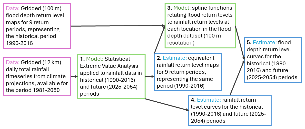
Figure 2 Diagram illustrating the methodology used to quantify the hazard information required for the risk estimation in this study. Specifically, this details the data, modelling and estimating steps taken to provide the required historical and future flood depth return-level curves at each location.

In the absence of open-source hydrological model output to represent all of the hazard information required, this approach offers a pragmatic and transparent method for quantifying this information, leveraging openly available, state-of-the-art datasets. It is, however, important to acknowledge several caveats and limitations. An important caveat of this approach is that the relationship between rainfall and flood depth is represented using a statistical mapping rather than a physically based hydrological model. This mapping is not explicitly validated against observed flood events or hydrological simulations and therefore may not fully capture key processes such as runoff generation, river routing, floodplain storage, and local flood defences. As such, the methodology is suited for demonstration purposes and raising awareness. A comprehensive discussion of the method's limitations is integrated throughout, with a summary of the key limitations presented in Sect. 5 for clarity.

Rainfall Extreme Value Spatial Model

Step 1 in Fig. 2 develops a model to estimate the continuous return-level curve for rainfall across the entire study region. This model enables us to characterise rainfall extremes for both time periods considered in the analysis: historical (1990–2016) and future (2025–2054), providing a foundation for assessing flood hazard consistently over time. Due to the limited (∼ 30-year) record length in each time slice, empirical estimation of rare high return-period events beyond the 1-in-30-year event is not reliable, necessitating the use of a statistical model. This is achieved using a spatial extreme value statistical model applied to the 12 km gridded climate model projections of daily total rainfall introduced in Sect. 2.2.2. Extreme Value Analysis is a branch of statistics used to understand and model rare, extreme events (Coles, 2001), and is therefore particularly suited to representing high return-periods (e.g. 1 in 100-year events) as is required here.

Specifically, our model structure follows the approach detailed in Youngman (2022), namely, an Extreme Value Generalised Additive Model (EV-GAM). We use a Generalised Pareto Distribution (GPD) peak-over-threshold approach for modelling extreme daily rainfall, and penalised regression splines via a Generalised Additive Model (GAM) framework to model the spatial variability of the GPD parameters (Youngman, 2022). This GPD distribution choice is consistent with extreme value theory, which shows that exceedances above sufficiently high thresholds converge to a GPD (Pickands–Balkema–de Haan theorem). As such, EV-GAMs have been used to model environmental variables in a number of recent studies. These include Youngman (2019), who apply a peak-over-threshold EV-GAM to estimate return-levels for extreme wind gusts in the United States; Chan et al. (2023), who use a point process EV-GAM to produce updated projections of extreme rainfall using the latest UK climate data; and Brown (2020), who use a peak-over-threshold EV-GAM to model extreme temperature and investigates how climate change is projected to intensify heatwaves.

In this application, similar to a combination of Youngman (2019) and Chan et al. (2023), our model is specified such that at any given location the distribution of excess rainfall (greater than the local 98th percentile of non-zero rainfall) is represented using a GPD. This model incorporates a spatially varying scale parameter, which captures the dispersion or spread of the distribution and how it varies across space, and a shape parameter which remains constant across space, characterising the heaviness of the distribution's tail.

Holding the shape parameter constant in space is common practice in spatial modelling, because it has high sensitivity to small fluctuations in the data. Granting it too much flexibility can result in unstable and unreliable estimates, ultimately compromising the robustness of the model. This assumption is typically most suitable in applications where the spatial domain is moderate in size and where systematic, large-scale variation in higher-order distributional properties (such as skewness or tail behaviour) is not expected. While there may be genuine spatial variation in the rainfall tail behaviour within our study region (e.g., due to orography), evidence from spatial extremes modelling shows that adding unnecessary spatial flexibility to higher-order parameters risks overfitting and poor tail dependence characterisation; robust practice prioritises parsimonious marginal models over highly parameterised, spatially varying shapes (Davison et al., 2012). Consistent with this, our model checking does not provide evidence that allowing the shape parameter to vary spatially would materially improve the fit.

The spatial variation of the scale parameter is modelled using a GAM framework. In this approach, the dependence on spatial location (longitude and latitude) and mean rainfall is represented using penalised regression splines, forming a semi-parametric model that allows smooth spatial variation without imposing a rigid functional form. The model is fitted directly to rainfall data on the native 12 km × 12 km rotated latitude–longitude grid of the UKCP18 regional climate model, with each grid cell treated as an individual observation location. The spatial coordinates are standardised (centred and scaled) prior to modelling to improve numerical stability, while preserving the relative spatial structure of the data. As described by Chan et al. (2023), this EV-GAM method captures spatial inhomogeneity explicitly while ensuring spatial smoothness through the inclusion of spatial and geographical covariates (i.e. longitude, latitude and mean precipitation intensity). In addition, by using all available data across space (rather than modelling individual locations), it yields more robust estimates of extreme events at high return-periods as the model is able to borrow information about extremes from other locations across space. More detail, including the mathematical equations that summarise this model, are given in Sect. S1.1 of the Supplement.

Distribution parameters are assumed to be stationary within each defined time period (historical/future), primarily to ensure consistency with the underlying flood hazard modelling framework (Baugh et al., 2026), which does not include time-varying parameters. Further, this assumption is consistent with common practice in climate impact assessments where periods are treated as quasi-stationary representations of a given climate state (Herger et al., 2015; Schleussner et al., 2016; Kennedy-Asser et al., 2021; Garry et al., 2021; Dawkins et al., 2023a), and this assumption reflects the absence of a clear monotonic temporal trend in the rainfall distributions analysed here, consistent with previous findings (e.g. see p. 384 of Wood, 2017).

The model is implemented using the R statistical programming package evgam (Youngman, 2022), which is available for public download via the R CRAN repository. This package fits models using maximum likelihood estimation, and provides a set of EV-GAM parameter estimates, which can in turn be used to estimate return-levels associated with any given return-period.

Here, we fit separate models to:

• Each time period: historical (1990–2016) and future (2025–2054)

• Each of the 12 UKCP18 regional climate model ensemble members

• Each season: Spring (March, April, May), Summer (June, July, August), Autumn (September, October, November) and Winter (December, January, February)

These subsets of the rainfall data (e.g. historical winters from ensemble member 01) are modelled separately because the statistical behaviour of different combinations are expected to vary substantially. For instance, the spatial distribution of winter rainfall is likely to differ from that of summer rainfall. An alternative, more complex approach would involve modelling all data jointly, incorporating additional terms to account for variation across time periods, ensemble members, and seasons within a unified statistical framework. While this would increase model complexity and impose assumptions such as smooth transitions across seasons, it presents a potential avenue for future research aimed at enhancing the parsimony and elegance of the methodology.

Figure 3 shows a summary of some of the EV-GAM inputs and outputs over the study domain for one modelled combination: the historical period, UKCP18 ensemble member 01 and summer rainfall. This shows how the characteristics of rainfall vary over the region and how this is captured in the EV-GAM. For example, this shows how the 98th percentile of wet-day rainfall (Fig. 3a) and the mean rainfall (Fig. 3b) inputs are highest along the west coast of the UK and Norway, and how this is captured in the EV-GAM through the GPD scale parameter, which is higher in these regions (Fig. 3c), subsequently leading to similar spatial variation in the 1-in-100-year return-level for historical summer-time daily rainfall estimated from the model (Fig. 3d).

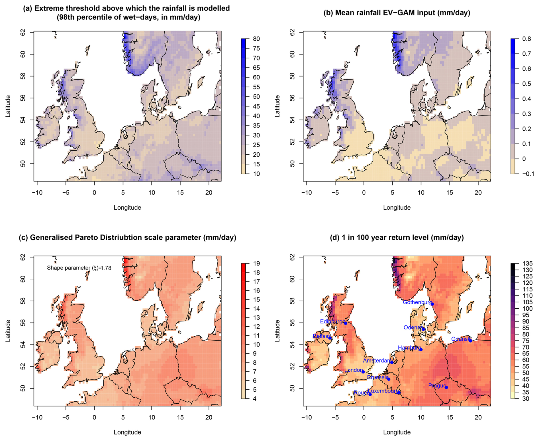
Figure 3 Spatial maps of key parameters in the extreme value analysis model for the historical period, UKCP18 ensemble member 01 and summer rainfall. These include (a) the rainfall threshold above which extremes are modelled (98th percentile of wet days), (b) the mean daily total rainfall over the modelled time period, scaled by taking away its median and dividing by its range (an input of the spatial variability in the EV-GAM scale parameter), (c) the fitted Generalized Pareto Distribution scale parameter, and (d) the estimated 1-in-100-year return-level for daily total rainfall (mm d⁻¹) across the European study region. The fitted Generalized Pareto Distribution shape parameter (which is constant in space) is also shown in panel (c), and the 12 European cities used for demonstration in later figures are shown in panel (d).

For illustration throughout this paper, we present detailed examples of the modelling workflow using a selection of grid cells identified as flood-prone in the CEMS flood hazard maps. To provide geographical context, we choose grid cells located closest to the central longitude-latitude coordinates of twelve European cities. These city grid cells were selected to span the study region and to capture a range of flood-risk conditions. Their locations are shown in Fig. 3d, and Table 1 lists their corresponding coordinates, sourced from an openly accessible dataset hosted on GitHub (ofou, 2018). It is important to note that the grid cells representing these cities differ across the hazard datasets: the rainfall dataset uses grid cells of 12 km × 12 km (e.g. as in Fig. 4), whereas the flood hazard dataset uses much finer 100 m × 100 m cells. Consequently, the flood hazard city grid cells shown only represent a small central portion of each city (e.g. Fig. 6 onward). For context, Table 1 provides information about the approximate size of each city (based on municipality regions) and how much of the city would be contained within each of these city grid cells of different scales. Figure S1 in the Supplement shows maps of four of these cities, demonstrating the location and relative size of the 100 m × 100 m grid cells.

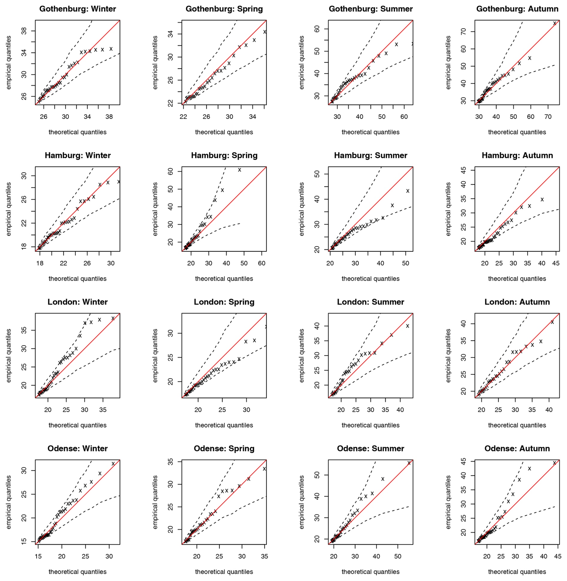
Figure 4 Statistical model validation plots: Quantile–Quantile (Q–Q) plots for the EV-GAM fitted to the historical period and UKCP18 ensemble member 01. Individual Q–Q plots are shown for models representing each season and for 4 12 km × 12 km grid cells co-located with the centre of 4 European cities (see Table 1). The black crosses show the relationship between the empirical quantiles of the UKCP18 rainfall data used to fit the EV-GAM (shown on the y axis) and the mean estimate of the corresponding theoretical quantiles from the EV-GAM fitted to this data (shown on the x axis). The dashed black lines show the 95 % confidence interval around this mean estimate from the EV-GAM, and the red line is the line of y = x.

Table 1 Municipal areas and coordinates of the twelve European cities selected to illustrate the modelling workflow, together with the approximate percentage of each city encompassed by co-located grid cells from the flood hazard dataset (100 m × 100 m) and the rainfall dataset (12 km × 12 km). These values contextualise the scale contrast between datasets and demonstrate how the flood hazard city grid cells shown in later figures capture only small central portions of each city. Figure S1 shows maps of four of these cities, demonstrating the location and relative size of the 100 m × 100 m grid cells. The final column shows the total non-residential property value in the respective grid cells (see Sect. 2.3.3 and Fig. 8c).

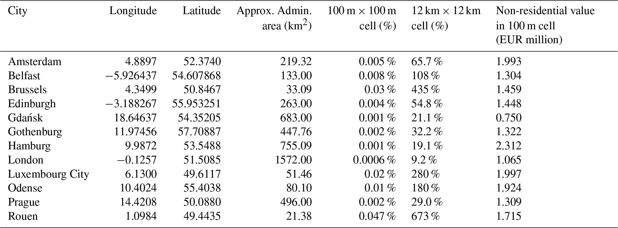
Figure 4 presents a series of model validation Quantile–Quantile (Q–Q) plots based on the historical period and UKCP18 ensemble member 01, for each season and four city grid cells within the study region. Equivalent Q–Q plots for the other combinations of time period and ensemble member are provided in Sect. S1.2. Q–Q plots are a standard model validation technique in statistical modelling for assessing whether the empirical data follow a particular theoretical distribution. In this case we compare the quantiles of the UKCP18 rainfall data (y axis) against the quantiles of the GPD distribution fitted to that location and season via the EV-GAM (x axis). A perfect fit would be characterised by all points on the Q–Q plot lying exactly along the line y = x. In practice, perfect alignment is rare and a model fit is generally considered to be good if the points lie within the 95 % confidence interval (i.e. any deviations from the theoretical distribution are within expected random variation).

Figure 4 shows that, for each example grid cell and season the quantiles of the empirical data sit within the 95 % confidence interval of the statistical model, indicating a good fit. The same is true for the other combinations of time period and ensemble member (see Sect. S1.2). In some cases in Fig. 4, however, such as for the Hamburg grid cell in the summer, many of the quantile points sit close to one end of the 95 % confidence interval. While this could potentially indicate systematic over- or under-estimation in some cases, it more plausibly reflects the increased uncertainty associated with representing rare extremes from limited samples. This behaviour is well-known in extreme value analysis and does not indicate systematic bias in the model. While good model fit is still achieved in these cases (points fall within the 95 % confidence interval), valuable future work could aim to refine the EV-GAMs to improve upon this, for example by including additional covariates within the spatial model for the GPD scale parameter such as the proximity to the sea, prevailing wind patterns and land-use characteristics. Section S1.2 also provides further model validation plots for the full spatial region, demonstrating that the models perform well.

To accurately represent the complete return-level curve for rainfall for any given location across the entire year (rather than representing each season in isolation) we combine simulated rainfall data from all four seasonal models and compute the relevant return-levels. For each time period and climate model ensemble member, we use the parameter estimates from the EV-GAM models to generate daily rainfall simulations. Specifically, we simulate 10 000 d from each seasonal model, resulting in a combined dataset of 40 000 daily rainfall values that represent rainfall from the whole year for that time period and ensemble member. This comprehensive set of simulations allows us to estimate any desired return-level by identifying the corresponding quantile from the full-year set of samples. Importantly, appropriate adjustments are applied to these quantiles to account for the peak-over-threshold framework and the fact that only the upper portion of the rainfall distribution is simulated; these adjustments are described in detail in Sect. S1.3.

Step 2 of the hazard methodology (Fig. 2) estimates rainfall return-levels across all locations, corresponding to the nine return-periods provided by the flood depth hazard maps from the CEMS database (introduced in Sect. 2.2.1). These return-periods are 1-in-10, 20, 30, 40, 50, 75, 100, 200, and 500 years, and represent the historical period (1990–2016). Figure 5 illustrates the resulting rainfall return-level maps for UKCP18 RCM ensemble member 01. As expected, the magnitude of daily rainfall (i.e. the return-level) increases with longer return-periods (i.e. as the events become more infrequent). This trend is consistent across all locations within the study region. Notably, areas with the highest rainfall return-levels, such as western UK and Norway, remain prominent across all return-period maps, highlighting the persistently high rainfall hazard characteristics in these regions.

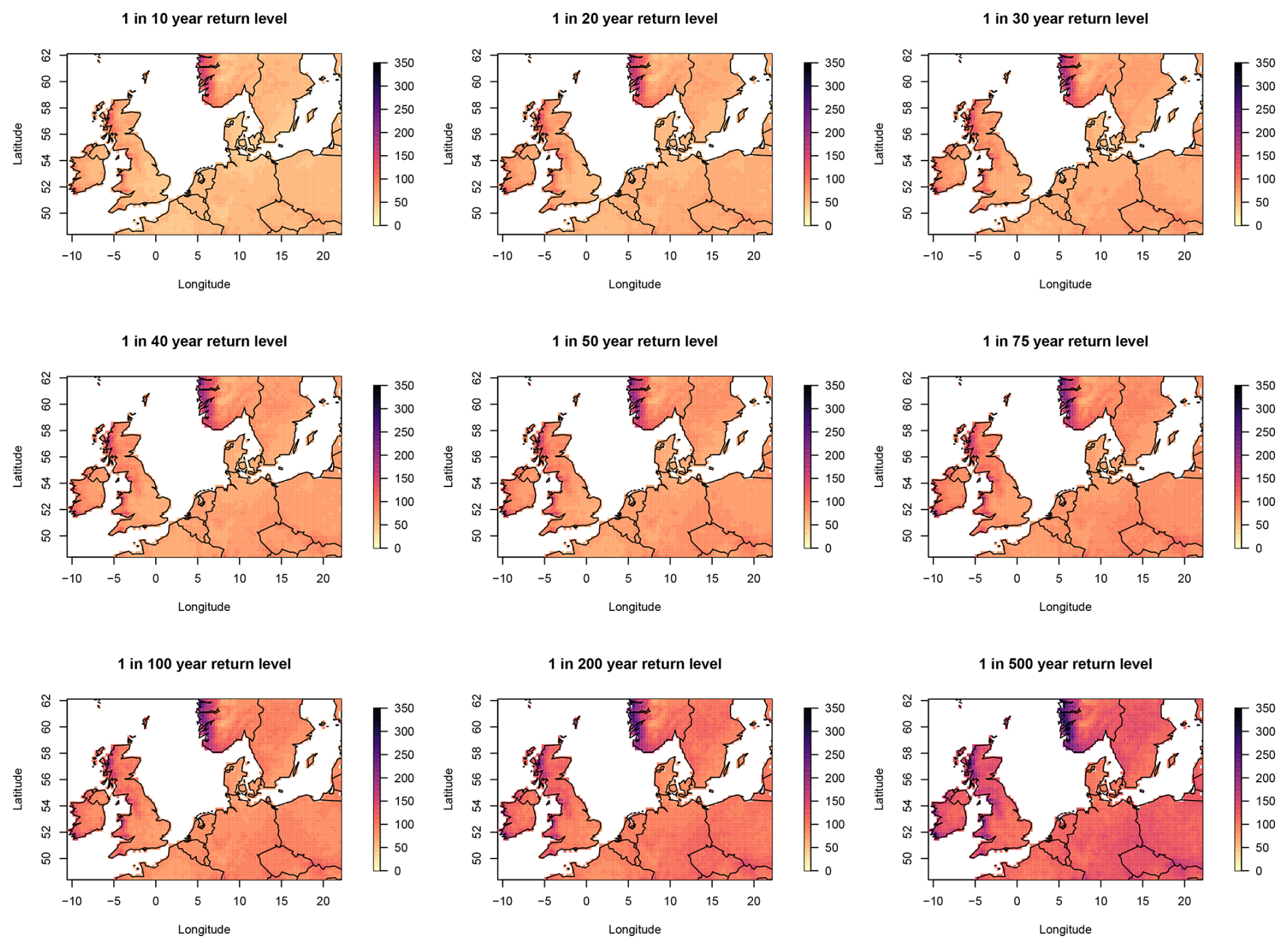
Figure 5 Spatial maps of rainfall return-levels (mm d⁻¹) across Europe for nine return-periods (10, 20, 30, 40, 50, 75, 100, 200, and 500 years) based on historical (1990–2016) daily total rainfall data from UKCP18 RCM ensemble member 01.

Relating rainfall and flood depth return-levels

Step 3 of the hazard methodology (Fig. 2) focuses on modelling the relationship between the rainfall distribution and flood depth distribution at each location. This mapping allows for any flood depth quantile associated with any return-period in either the historical or future periods to be estimated (as is required for the hazard component of this risk assessment). Here this is done by fitting a monotonically increasing cubic spline to the relationship between historical rainfall return-levels (from Step 2) and flood depth return-levels (taken from the CEMS flood hazard maps, introduced in Sect. 2.2.1).

Rainfall return-levels are modelled at the 12 km spatial resolution of the UKCP Regional Climate Model (RCM), while flood depth return-levels are provided at a much finer resolution of 100 m. To establish the mapping between rainfall and flood depth, each flood depth grid cell is paired with its geographically nearest rainfall grid cell. As a result, multiple flood depth grid cells share the same rainfall grid cell for this mapping, reflecting the coarser resolution of the rainfall data.

Here, a spline is fitted to each relevant 100 m × 100 m flood hazard grid cell and corresponding rainfall grid cell separately using the scipy.interpolate.PchipInterpolator function in the Python SciPy library. This function creates a smooth curve that passes through a given set of data points, preserving the shape and monotonicity of the data (see Fig. 6). This spline fitting is carried out for each of the UKCP18 RCM ensemble members individually, allowing for a quantification of climate model uncertainty in the resulting risk.

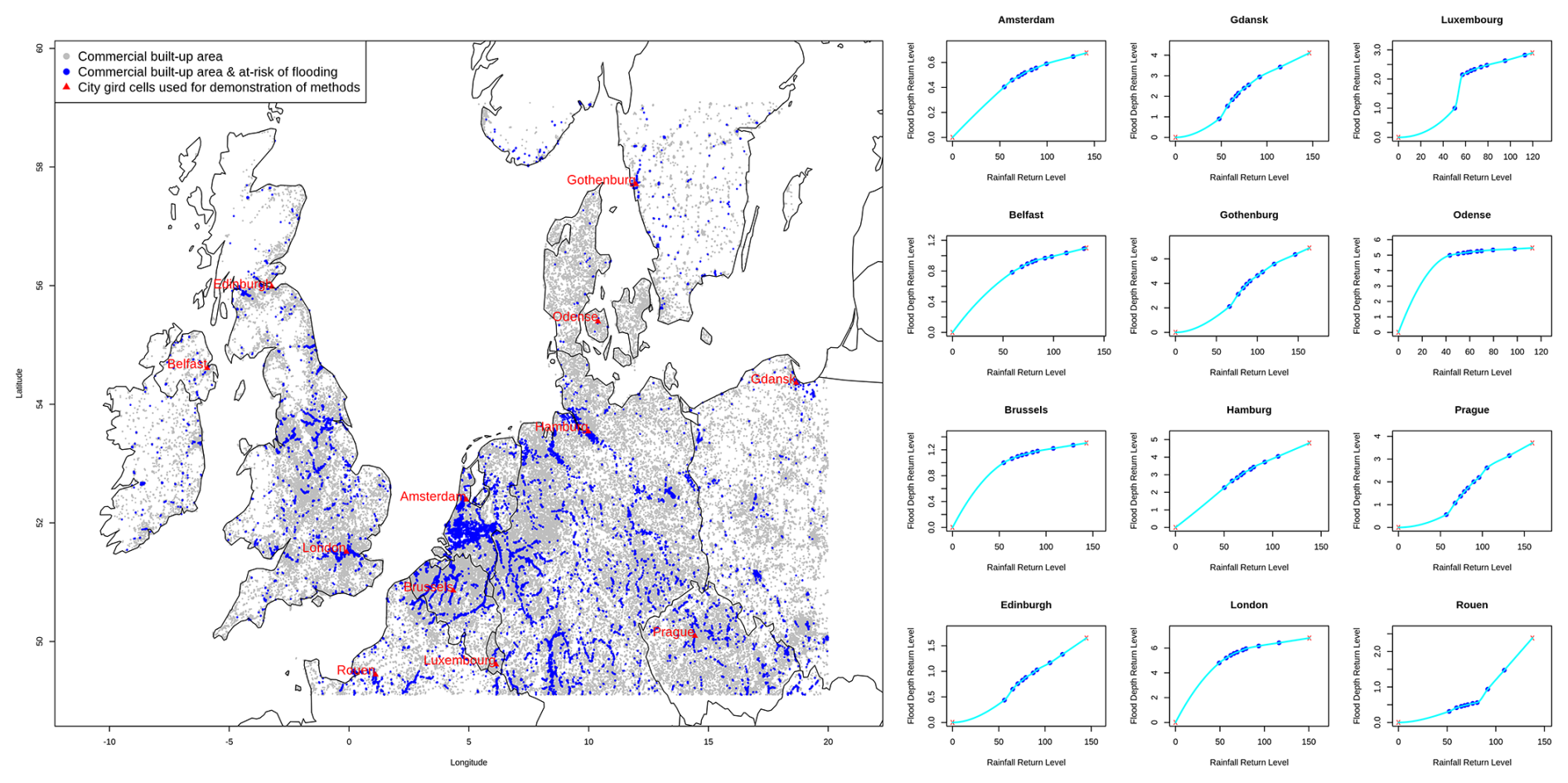
Figure 6 Left panel: a map of the North-West Europe region used within this study, with points added to show the 100 m × 100 m grid cells in the flood hazard and exposure datasets that meet two criteria: (1) shown in grey – viable candidates for inclusion in synthetic pension portfolios, containing a minimum of 1000 m² of built-up non-residential property (see Sect. 2.3.1 for more information); and (2) shown in blue – viable candidates also at risk of flooding, indicated by non-zero flood depth for events up to at least the 1-in-75-year return-period in the CEMS flood hazard dataset. Right panel: spline-based curves linking rainfall intensity (mm d⁻¹) to flood depth (m) for 100 m × 100 m grid cells representative of the centre of 12 European cities (locations shown on the map in the left panel, see Table 1 for more detail). The blue points show the relationship between the nine flood depth return-levels taken from the CEMS flood hazard dataset (y axis, see Sect. 2.2.1) and the equivalent values for the rainfall (x axis) estimated in Step 2 of the methodology shown in Fig. 2 (here shown for the model based on historical rainfall data from the UKCP18 RCM ensemble member 01). The red crosses indicate two additional points included in the spline fitting to enable extrapolation beyond the nine quantiles: one at the origin (0,0), i.e. no rain = no flood, and one at the maximum rainfall across the combined historical and future periods. The associated maximum flood depth is estimated by linearly extrapolating from the gradient of the two highest historical points, ensuring stable, monotonic, and physically consistent behaviour. The extrapolated portion of the spline is tightly constrained by the imposed bounding points. While sensitivity to these assumptions could be explored, this lies beyond the scope of the present idealised analysis, which focuses on a single, physically consistent specification.

Rather than modelling every 100 m × 100 m grid cell of the flood depth hazard maps within the study region, we concentrate on those that meet two criteria: (1) they are viable candidates for inclusion in our synthetic pension portfolios, containing a minimum of 1000 m² of built-up non-residential property (see Sect. 2.3.1 for more information); and (2) they are at risk of flooding, indicated by non-zero flood depth for events up to at least the 1-in-75-year return-period in the CEMS flood hazard maps. In the left panel of Fig. 6, the grey points represent locations that meet criterion (1), and blue points satisfy both criteria (1) and (2). These blue points are therefore the ones for which the rainfall-to-flood-depth mapping is performed.

The right panel of Fig. 6 shows the fitted monotonically increasing cubic splines for the 100 m × 100 m grid cells located within the centre of 12 European cities (all of which satisfy both of the modelling criteria, see Table 1 for more detail). In this figure the rainfall return-levels were estimated using the EV-GAM fitted to UKCP18 RCM ensemble member 01, and equivalent functions are also fitted to each of the other UKCP ensemble members. The shapes of the spline functions vary across the grid-cell locations, as may be expected given the differing flood characteristics of each area.

It is important to emphasise that this approach does not assume a direct event-based 1:1 correspondence between rainfall and flood events. Rather, it represents an idealised quantile-to-quantile mapping between rainfall and flood return-level distributions. In practice, related assumptions are commonly made in engineering “design event” approaches, where rainfall events of a given return-period are used to estimate flood magnitudes of the same nominal return-period (e.g. Kourtis et al., 2020). However, in reality, flood frequency curves arise from the integration of the full spatio-temporal rainfall distribution with catchment processes, and multiple rainfall events with differing characteristics can produce similar flood magnitudes. As such, the relationships derived here represent a simplified statistical approximation of a highly complex physical system. They do not explicitly account for key hydrological processes and are not validated against independent flood observations or model output. Consequently, this approach should be interpreted as a monotonic, first-order approximation of the relationship between rainfall and flood extremes, intended to enable large-scale analysis in the absence of consistent open hydrological datasets, rather than a physically complete or decision-ready representation of flood hazard for a particular location.

A further caveat arises from the mismatch in spatial resolution between the rainfall and flood depth datasets used (as described above). As a result, multiple flood-exposed locations may share identical rainfall return-levels despite experiencing different flood dynamics, adding further uncertainty to the derived relationships. The quantile-to-quantile mapping therefore implicitly assumes that rainfall statistics at the coarser climate model scale are representative of the local hydrological forcing relevant for each flood-prone grid cell. In reality, sub-grid-scale variability in rainfall, land cover, drainage, and topography can lead to substantial heterogeneity in local flood response that cannot be resolved at the climate model resolution. This mismatch may also introduce systematic bias, for example where convective rainfall extremes are smoothed at 12 km resolution, potentially leading to underestimation of localised flood-generating intensities. Despite this limitation, the approach remains suitable for capturing large-scale patterns of hazard and relative risk, as the quantile-mapping framework preserves the relative ordering of extreme events across space. This enables consistent comparison of hazard severity between regions, even if absolute local flood magnitudes are uncertain. Future work could reduce this limitation through higher-resolution climate data or explicit hydrological modelling. This scale inconsistency reinforces the interpretation of the approach as a large-scale approximation rather than a site-specific flood hazard assessment.

Figure 7 provides an illustration of the rainfall-to-flood mapping process for two 100 m × 100 m grid cells located within the centres of Gothenburg and Edinburgh respectively. Panels (a) and (c) show the historical and future rainfall return-level curves derived from the statistical extreme value models as per Step 4 of the hazard methodology schematic in Fig. 2. The historical curves align well with the National Oceanic and Atmospheric Administration (NOAA) historical records, which indicate that the empirical 1-in-60-year rainfall event is 86 and 82 mm d⁻¹ for Gothenburg and Edinburgh respectively (shown in Fig. 7a and c). These rainfall return-level curves are then combined with the location-specific spline functions (Fig. 6, here shown for UKCP18 RCM ensemble member 01) to estimate the corresponding flood depth return-level curves (Step 5 in Fig. 2), shown in Fig. 7b and d. This interpolates the continuous historical flood depth curve, filling in the gaps between the nine available data points from the CEMS flood hazard map database. Similarly, the future rainfall return-levels are used to generate the continuous future flood depth curve.

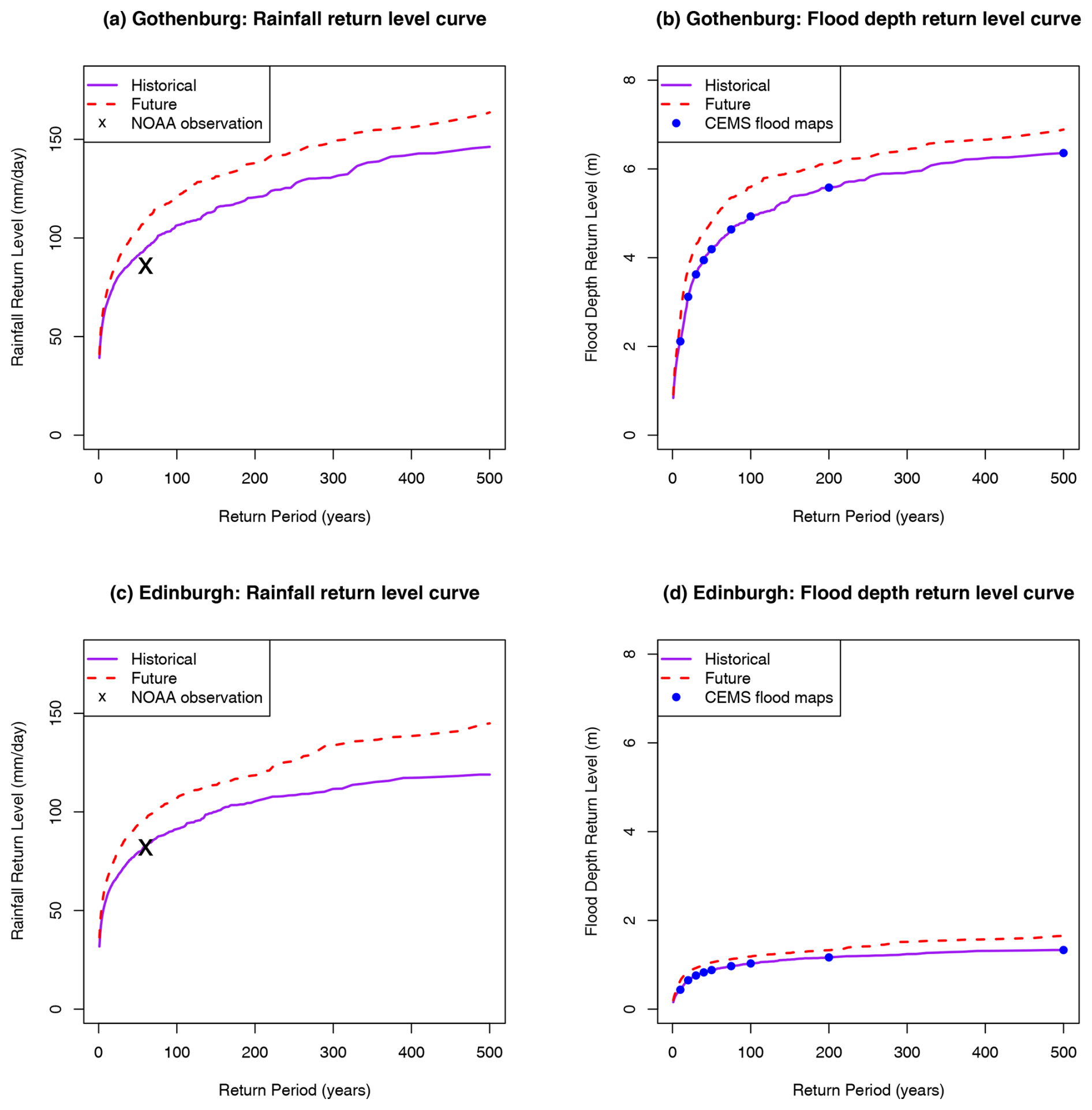
Figure 7 Illustration of the rainfall-to-flood distribution mapping process for two 100 m × 100 m grid cells located within the city centres of Gothenburg and Edinburgh (see Table 1 for more detail). Panels (a) and (c) show historical and future rainfall return-level curves derived from statistical extreme value models. The National Oceanic and Atmospheric Administration (NOAA) historical records for empirical 1-in-60-year rainfall events are shown for context. These curves are combined with location-specific spline functions (as in Fig. 6, here for UKCP18 RCM ensemble member 01) to estimate flood depth return-level curves. Panels (b) and (d) display the resulting historical and future flood depth curves, including the original nine return-levels for historical flood depths taken from the CEMS flood maps.

It should be noted that this approach assumes the rainfall–flood mapping is stationary across the two time periods. That is, while rainfall extremes are allowed to change between historical and future periods, the statistical relationship used to map rainfall return-levels to flood depth return-levels is held fixed. As such, the projected changes in flood hazard arise from changes in rainfall extremes rather than changes in the rainfall–flood mapping itself. Explicitly modelling such non-stationarity would require physically based hydrological and hydrodynamic models driven by high-resolution climate data, which are not consistently available as open datasets at continental scale, as discussed in Sect. 2.2.1.

Figure 7b and d show the fitted continuous flood depth return-level curves for both the historical and future periods alongside the original CEMS flood map data points used in the spline fitting. By construction, the historical flood depth curves pass through these data points, and therefore the close alignment reflects the successful spline interpolation approach. The same fitted relationships are then applied to the future rainfall return-levels, allowing the estimation of corresponding future flood depth return-level curves. We note that for Gothenburg, the historical and future flood depth return-level estimates for return-periods greater than 100 years appear notably high (reaching in excess of 5 m). These values closely reflect the corresponding CEMS flood map estimates, which themselves exhibit relatively large flood depths for high return-periods in this grid cell. Although previous flood modelling work for Gothenburg has reported water depths in excess of 2 m (Filipova and Rana, 2012), this discrepancy suggests that the known caveats associated with the CEMS dataset (discussed in Sect. 2.2.1) may be contributing to an overestimation of flood depths at this location.

The same approach is used to estimate the continuous return-level curve for historical and future flood depth at all potential portfolio location 100 m grid cells at-risk of flooding within the study region (blue points in the left panel of Fig. 6). These modelling steps are then applied to each of the UKCP18 RCM ensemble members individually, resulting in a representation of the full flood depth return-level curve (distribution) for:

• each time period – historical (1990–2016) and future (2025–2054),

• each of the 12 UKCP18 RCM ensemble members.

Equivalent graphs to those shown in Fig. 7 but for all ensemble members are shown in Fig. S2.

2.3 Exposure

The exposure component of the risk assessment necessitates an estimation of the monetary value of assets at risk. While our approach can accommodate a range of property types, this study specifically focuses on portfolios that are heavily invested in large commercial real estate. Due to the lack of detailed data on the precise location and valuation of assets held by these types of pension funds, exposure is approximated here using a combination of spatial information about non-residential property.

2.3.1 Built-up surface data

The GHS-BUILT-S R2023A dataset, developed by the European Commission's Joint Research Centre, offers a high-resolution, multi-temporal raster grid of global built-up surface estimates. It spans 1975 to 2030 in 5-year intervals, enabling consistent spatial analysis of urbanisation trends over time (Pesaresi and Politis, 2023; Pesaresi et al., 2024). The dataset provides both total and non-residential built-up surface (predominantly commercial buildings). To reflect our choice to consider portfolios that are heavily invested in large commercial real estate, we use the non-residential built-up surface as a proxy for asset location and scale, providing a representative basis for our synthetic portfolio construction. Non-residential built-up data in GHS-BUILT-S R2023A is produced using a Symbolic Machine Learning method that combines Sentinel-2 and Landsat imagery with reference datasets such as OpenStreetMap and building footprints from Facebook and Microsoft (Pesaresi et al., 2024). The approach enables sub-pixel estimation of built-up surfaces and separates residential from non-residential areas using spatial patterns, land-use indicators, and auxiliary data. The classification shows high accuracy, and the model infers historical growth trends to extrapolate built-up surfaces to 2030.

This data is available at a 100 m spatial resolution over land and aligns with the grid cell locations used in the flood-depth hazard maps (introduced in Sect. 2.2.1). Each grid cell value represents the number of square meters of built-up surface within that cell, which has an area of 10 000 m². The data is supplied as global TIFF raster tiles, each covering 5° × 5° in WGS84 (EPSG:4326). For this study, we use three tiles covering the UK, Belgium, the Netherlands, Denmark, and parts of France, Germany, the Czech Republic, Poland, Norway, and Sweden (see Fig. 6, left panel). Future work could extend this to larger or alternative regions depending on user needs.

We use data representative of the year 2020. This reference year was selected as it closely reflects the contemporary built environment at the time of the GHS-BUILT-S dataset's publication. By anchoring our portfolios to a consistent spatial distribution from 2020, we are able to assess both historical (1990–2016) and near-term future (2025–2054) flood risk, ensuring that any observed changes in the risk are attributable to evolving hazard dynamics rather than shifts in portfolio composition, thereby isolating the impact of climate change on a fixed set of asset locations. Future work could explore how risk may vary if different representative years were used.

Finally, to capture larger commercial properties within the synthetic portfolios we only use the built-up surface information from those locations that have at least 10 % of the grid cell containing non-residential buildings (i.e. at least 1000 m²).

2.3.2 Property value data

In addition to characterising the location and extent of non-residential property, to assess flood risk in financial terms it is necessary to translate these physical attributes into monetary values. This requires data on property values across the region of interest, allowing for the estimation of the economic exposure of assets represented in our synthetic portfolios.

For this, we use open-source information from the European Commission's Joint Research Centre database on Global flood depth-damage functions (Huizinga et al., 2017). This database contains country specific estimates of the maximum building-based damage costs (in EUR per m²) for various land use categories, including residential, commercial, industrial, and agricultural areas. These maximum damage values are derived from construction cost surveys conducted by multinational construction companies.

For each European country in our study region, we represent the property value per m² (constant across that country) as the estimate of the maximum building-based damage costs (in EUR per m²) for commercial (i.e. non-residential) properties, to align with the use of non-residential built-up surface data as described in Sect. 2.3.1. Asset values per unit area are applied uniformly at the national level. This simplification does not capture intra urban or regional heterogeneity in property values, particularly within large metropolitan areas, and may therefore misrepresent absolute damages at specific locations. While property values undoubtedly vary within countries, we were unable to identify a suitable open-source dataset with sufficient spatial resolution to capture this variability. Nevertheless, we consider the approach adopted here to be a reasonable first step for this idealised demonstration.

2.3.3 Quantifying the total value of assets

Across the study domain, we quantify exposure (the total value of assets) by combining:

• 1.

  The location and physical footprint/size of non-residential built-up areas (described in Sect. 2.3.1 and shown in Fig. 8a). This metric is captured on a 100 m resolution spatial grid, and specifies the amount of square metres of built-up surface in each cell. Here only grid cells where this footprint exceeds 1000 m² within a 10 000 m² grid cell are considered in an effort to better represent larger commercial properties (i.e. grey points in the left panel of Fig. 6).

• 2.

  The country-wide property value per m² (described in Sect. 2.3.2 and shown in Fig. 8b).

These two quantities are multiplied together to provide an estimate of the total value of assets within each human settlement grid cell, as shown in Fig. 8c.

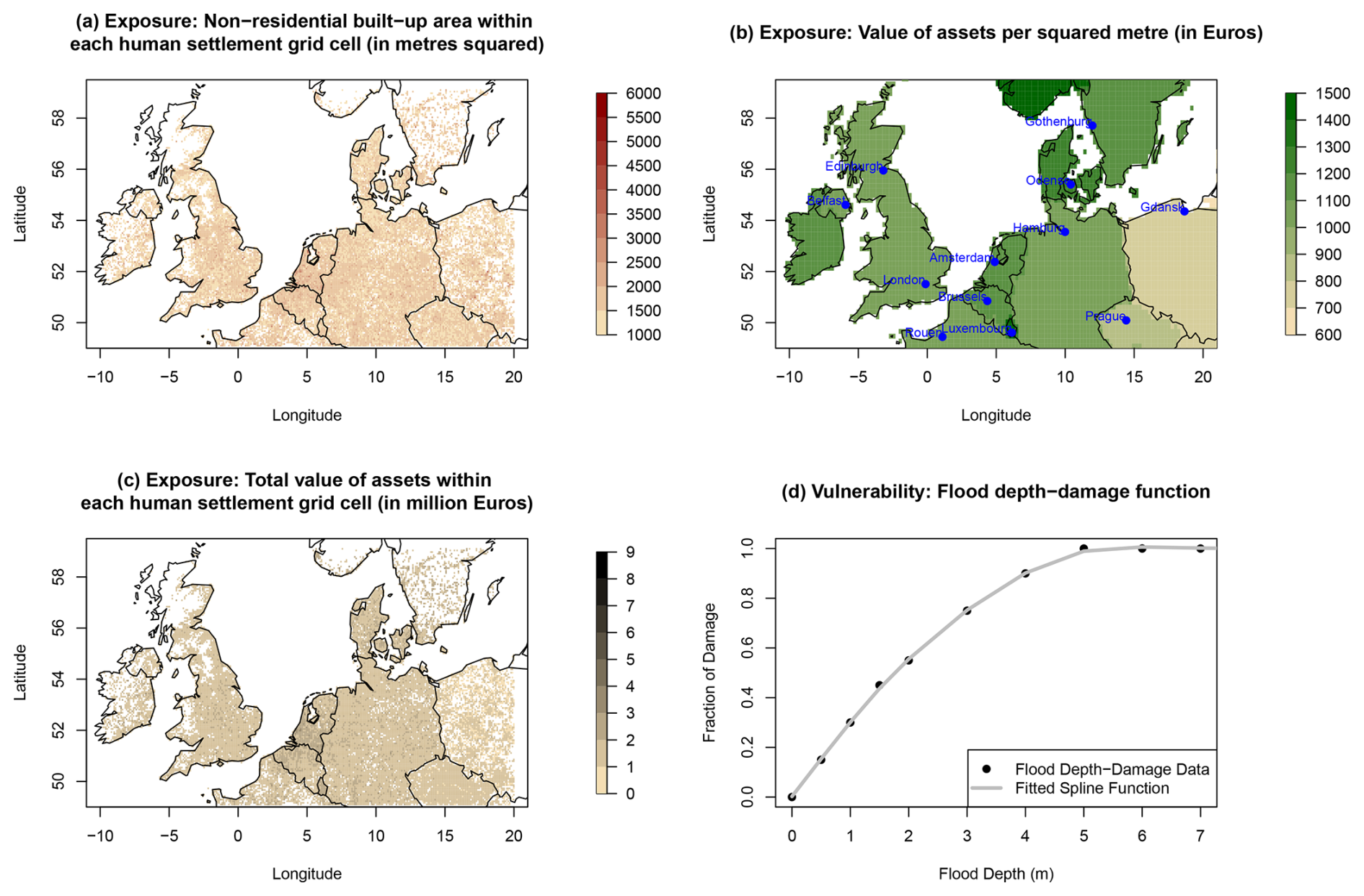
Figure 8 Exposure and vulnerability metrics. Panels (a)–(c) show the spatial distribution of exposure indicators for European human settlement grid cells: (a) non-residential built-up area within the 100 m × 100 m grid cell (in m²), (b) asset value per square metre (in EUR), and (c) total asset value within the 100 m × 100 m grid cell (in million EUR). Panel (d) illustrates the vulnerability function as the relationship between flood depth and damage (see Sect. 2.4 for more detail). Note that asset values per square metre in panel (b) are applied uniformly at the country level; spatial patterns therefore reflect national differences rather than within-country variability; a tabulated version of these values is available in the Global Flood Depth-Damage Functions database (Huizinga et al., 2017).

2.3.4 Constructing synthetic portfolios

The estimate of the monetary value of assets (Fig. 8c) is used to construct synthetic property portfolios. Based on advice from a researcher specialising in the pensions sector, portfolios containing 450 asset locations (grid cells) were considered. As shown in the left panel of Fig. 6, only a small proportion (specifically 7.5 %) of potential portfolio locations are at risk of flooding (i.e. blue points compared to grey points in this figure). As such, the level of flood risk associated with a particular portfolio will likely greatly depend on the proportion of the sampled 450 asset locations that are at-risk of flooding compared to not at-risk. This is explored further in Sect. 3.2.

Synthetic portfolios are created in two ways to explore idealised pension portfolio flood risk within this study:

• 1.

  Portfolio asset locations sampled randomly from all potential grid cells,

• 2.

  The proportion of at-risk and not at-risk locations is varied, and locations sampled at random to satisfy these proportions.

In the absence of detailed, openly available data on real financial portfolios, this synthetic approach provides a neutral and controlled framework for exploring the behaviour of the methodology. By avoiding underlying characteristics of real financial portfolios, the use of synthetic portfolios ensures that the resulting patterns of risk reflect the underlying hazard–exposure relationships rather than features specific to any individual portfolio. While the exact values may differ for real financial portfolios, the scientific conclusions and relative patterns of risk are not expected to depend strongly on whether portfolios are synthetic or real. Application to more realistic portfolios, where suitable data are available, represents an important direction for future work.

2.4 Vulnerability

To quantify vulnerability we employ a depth-damage function that estimates the proportion of an asset’s value likely to be lost, as a function of flood depth. Specifically, we use information obtained from the European Commission's Joint Research Centre database on Global flood depth-damage functions (Huizinga et al., 2017). This database provides a comprehensive set of damage curves for each continent, relating flood depth to economic damage for the same land use categories as the maximum damage cost data described in Sect. 2.3.2. The damage curves are derived from empirical data and expert judgment, and are designed to be compatible with large-scale flood modelling frameworks. They offer depth-damage relationships that estimate the proportion of asset value lost at different inundation depths, enabling consistent and scalable economic impact assessments of flooding events (Huizinga et al., 2017).

Here, the flood depth-damage relationship representative of commercial (i.e. non-residential) properties in Europe is used, again to align with the use of non-residential built-up surface data as described in Sect. 2.3.1. A representation of this curve is provided in Fig. 8d. The data is provided as a series of data points and a monotonically increasing cubic spline is fitted to the points to represent the complete vulnerability depth-damage function (using the spline model as in Sect. 2.2.3).

In the absence of more spatially resolved vulnerability data, this function is uniformly applied across all locations and assets within the study region. While this approach provides a useful baseline, future work and real-world applications would benefit from incorporating asset-specific vulnerability profiles.

2.5 Translating Hazard to Risk

For any given location/grid cell that is at risk of flooding, hazard, exposure, and vulnerability information can be combined to estimate flood risk. In this study, flood risk is represented by the Expected Annual Damage (EAD), which is defined as the expectation of flood damage over the full range of event probabilities:

$$\begin{array}{}\text{(1)}& {\displaystyle }\text{EAD}=\int D\left(h\right)\mathrm{d}p\left(h\right),\text{(2)}& {\displaystyle }D\left(h\right)=V\left(h\right)\times E,\end{array}$$

where h is the flood depth intensity, D(h) denotes the damage cost associated with a flood of depth h, and p(h) is the corresponding annual exceedance probability. The damage cost is expressed as the product of the vulnerability function, V(h), which maps flood depth intensity h to fraction of damage (see Fig. 8d), and the local financial exposure, E (here taken as the total value of assets; see Fig. 8c). The vulnerability function is applied deterministically to the hazard intensity, such that flood depths from the hazard return-level curve are translated directly into fractional damage (for example, a flood depth of 1 m corresponds to approximately 30 % damage at that location).

As the integral for EAD cannot generally be evaluated in closed form, it is approximated numerically. Here, this is achieved using the composite trapezoidal rule, implemented using the Python scipy.integrate.trapezoid function, evaluated at discrete annual exceedance probabilities corresponding to return-periods of 1–500 years at integer increments.

The annual exceedance probability (AEP), denoted p(h) in Eq. (1), is related to the return-period T under a Poisson assumption as,

$$\begin{array}{}\text{(3)}& \text{AEP}=\mathrm{1}-\exp (-\mathrm{1}/T),\end{array}$$

where T is the return-period in years. For rare events (i.e. large T), this expression approaches the commonly used approximation AEP ≈ $\mathrm{1}/T$. We note that the approximation AEP ≈ $\mathrm{1}/T$ would yield a maximum AEP of 1 at T  = 1; however, the Poisson-based formulation provides a more physically consistent representation of exceedance probability for frequent events. In this study, the lowest return-period considered is the 1-year event, corresponding to a maximum AEP of approximately $\mathrm{1}-\exp (-\mathrm{1})$ ≈ 0.631 under the Poisson assumption.

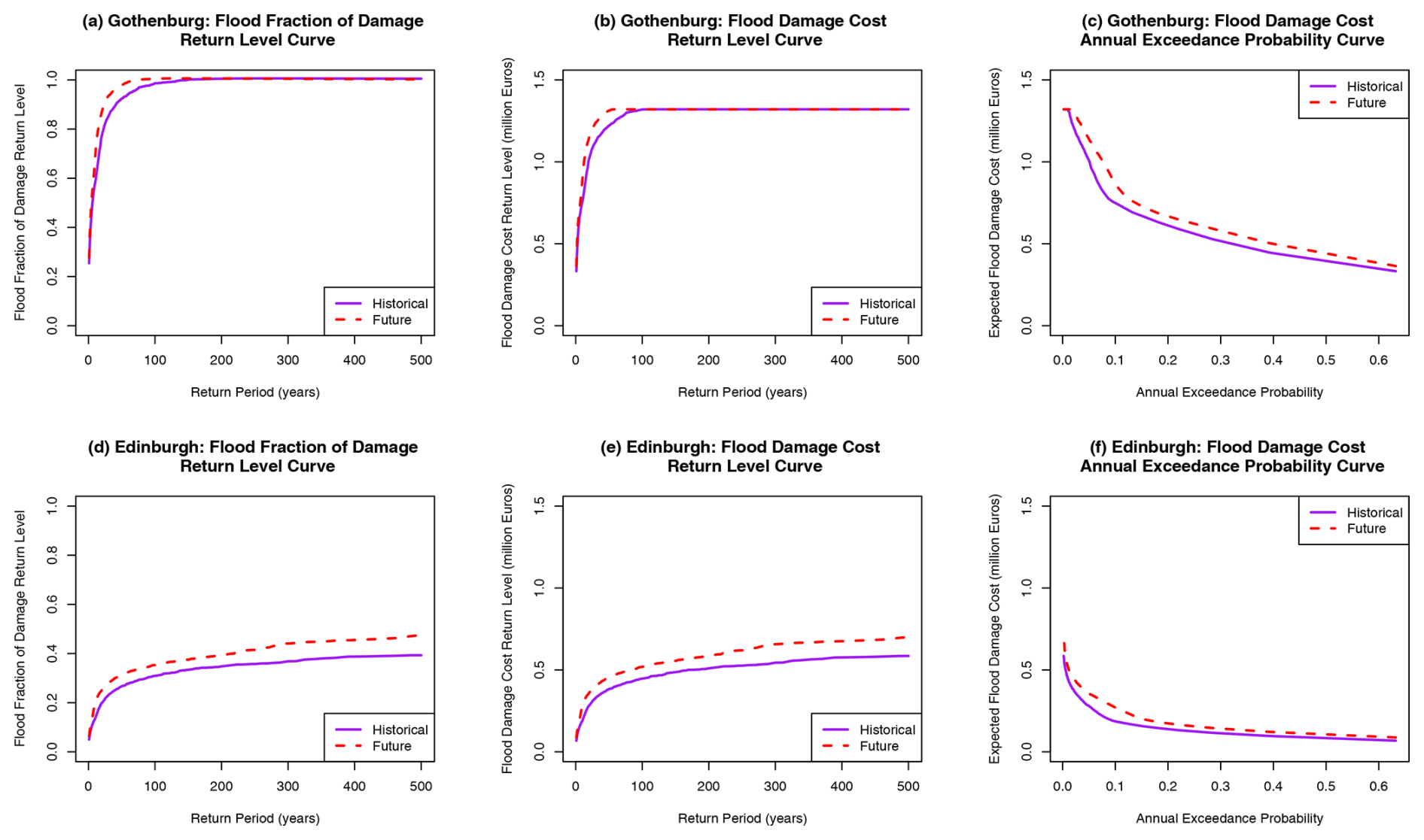
Figure 9 Illustration of the hazard-to-risk estimation process for two 100 m × 100 m grid cells representative of the city centres of Gothenburg and Edinburgh (see Table 1 for more detail). Panels (a) and (d) show historical and future flood fraction of damage return-level curves derived by applying the vulnerability function to the equivalent flood-depth return-level curves. Panels (b) and (e) show the historical and future flood damage cost return-level curves derived by multiplying the flood fraction of damage return-level curves by the exposure metric (total value of assets) in that 100 m × 100 m grid cell. Panels (c) and (f) show the corresponding Annual Exceedance Probability (AEP) curves derived by converting the x axis from return-period (T) to annual exceedance probability (AEP) using a Poisson assumption (Eq. 3). This example uses hazard information derived from UKCP18 RCM ensemble member 01.

Figure 9 demonstrates this risk estimation (for both the historical and future periods) for the 100 m × 100 m grid cells located within the city centres of Gothenburg and Edinburgh, using the hazard information derived from UKCP18 RCM ensemble member 01, and summarised in the following steps:

1. First, the vulnerability function, V(h) in Eq. (2), (represented by the flood depth–damage curve in Fig. 8d) is applied to the hazard (flood-depth) return-level curves (Fig. 7b and d), as described above, to derive the corresponding return-level curve for the fraction of flood damage. This is shown in Fig. 9a and d for Gothenburg and Edinburgh, respectively.

2. The flood fraction of damage values are then converted to damage costs by multiplying by the exposure value, E in Eq. (2), in that 100 m × 100 m grid cell (taken from Fig. 8c), as shown in Fig. 9b and e for Gothenburg and Edinburgh, respectively. These plots therefore quantify D(h) from Eq. (1) on the y axis. Note the relatively small size of the grid cells compared to the size of the cities as a whole (see Table 1 for more detail), which explains the magnitude of the flood damage costs (i.e. these values represent a small region within the city centre rather than the entire city).

3. Finally, the EAD is calculated by estimating the integral in Eq. (1). This is equivalent to estimating the area under the Annual Exceedance Probability (AEP) curve for flood damage costs, D(h). The AEP curves for flood damage costs for the Gothenburg and Edinburgh grid cells are shown in Fig. 9c and f, respectively. The AEP is defined as in Eq. (3). These plots quantify D(h) from Eq. (1) on the y axis and p(h) from Eq. (1) on the x axis, and the EAD is therefore estimated as the area under this curve via the composite trapezoidal rule, integrated along the AEP axis, as described above.

These steps are carried out for all viable synthetic portfolio 100 m × 100 m grid cells that are considered to be at risk of flooding (blue points in the left panel of Fig. 6). As with the hazard component, for comparison this is repeated for:

• each time period – historical (1990–2016) and future (2025–2054),

• each of the 12 UKCP18 RCM ensemble members.

3 Results

3.1 Quantifying historical and future physical risk

We begin by exploring the estimated idealised flood risk, expressed as Expected Annual Damage (EAD), across the entire study region for both the historical period (1990–2016) and the projected near-term future period (2025–2054), using the methodology outlined in Sect. 2. As described in Sect. 2.2.2, no bias correction is applied to the rainfall data used in this analysis. This, and a number of other modelling caveats (discussed in detail in Sect. 5), may affect the absolute magnitude of simulated rainfall extremes, and consequently the resulting flood depths and associated monetary estimates. As such, the absolute values of EAD should be interpreted with caution, with greater emphasis placed on the relative behaviour and spatial patterns of risk.

Figure 10a illustrates this risk in the historical and future periods for a selection of 100 m × 100 m grid cells located in the centre of 12 European cities (see Table 1 for more detail). These EAD estimates are calculated at the grid-cell scale and are intended to illustrate relative spatial variability in risk; they are not directly comparable to reported losses from individual real-world flood events, which typically reflect aggregated impacts over much larger spatial extents and depend on additional local factors. Figure 10a shows that there is flood risk (EAD) in the historical period, and that future EAD values are consistently higher than historical estimates across all city centre grid cells.

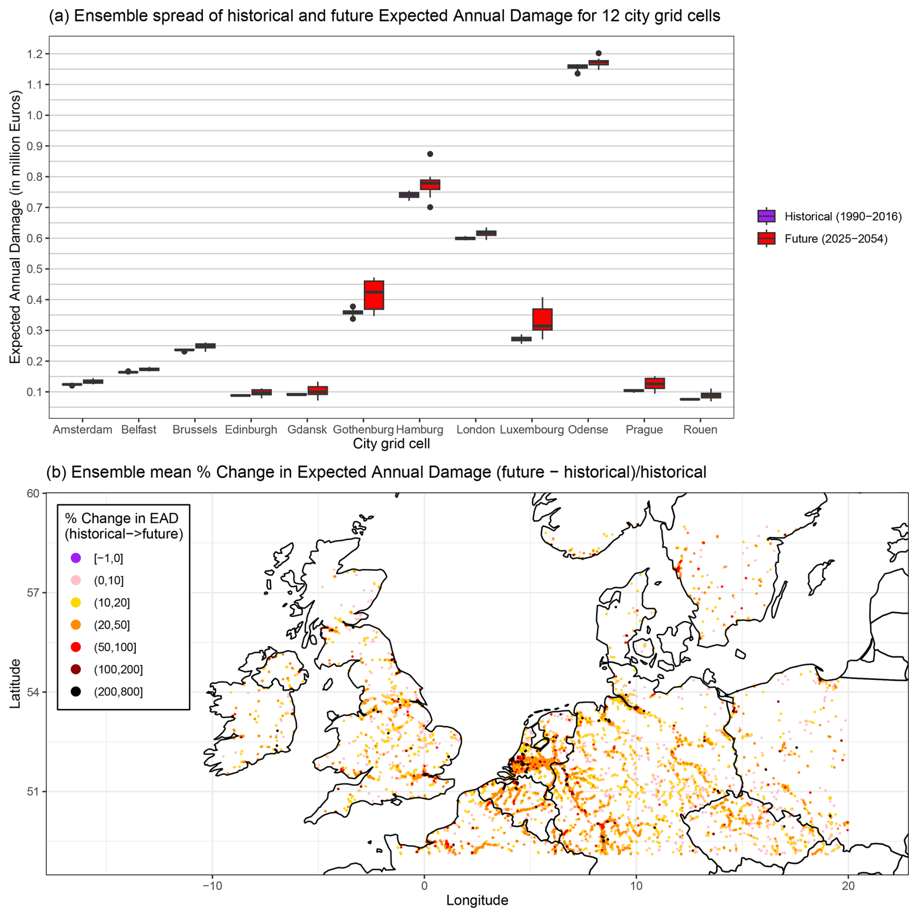
Figure 10 A comparison of historical and future flood risk, expressed as Expected Annual Damage (EAD) derived using the methodology described in Sect. 2: (a) UKCP18 RCM ensemble spread in EAD for 12 100 m × 100 m grid cells located in the centre of 12 European cities (see Table 1 for more detail) in historical (1990–2016) and future (2025–2054) periods. Boxes represent the interquartile range (25th–75th percentiles) of ensemble EAD, with the central line indicating the median; whiskers extend to 1.5 times the interquartile range, and points beyond this range are shown as outliers; (b) UKCP18 RCM ensemble mean percentage change in EAD between historical and future periods, calculated as (future EAD − historical EAD) $/$ historical EAD in each location. A value of this metric between 50–100 means the future EAD is 50 %–100 % greater than the historical EAD.

Figure 10b further demonstrates the upward trend in flood EAD between the historical and future periods. The map indicates widespread positive percentage increases in EAD across the study region, with only 0.1 % of at-risk locations showing no change or a decrease. This suggests that flood risk is projected to rise across almost the entire study area. Many locations exhibit increases exceeding 20 %, and some grid cells show particularly large changes, with increases of up to 800 % in the future period relative to historical conditions. It should be noted that future flood risk is evaluated only for locations identified as at-risk in the historical period. As a result, potential increases in EAD in newly exposed areas are not captured here, and future risk may therefore be underestimated.

In Fig. 10a, flood risk is particularly pronounced in the grid cells located within London, Hamburg, and Odense, suggesting that these locations may be especially susceptible to current and future flood-related economic losses. Figure 11 illustrates how the historical EAD in the 12 city centre grid cells relates to the two components of flood risk that vary by location: the hazard (summarised by the historical 1-in-100-year flood depth) and the exposure (total exposed asset value). For example, this figure highlights that, in the central London 100 m grid cell, the high historical EAD is primarily driven by high historical hazard. In contrast, the high EAD in Hamburg arises largely from the substantial concentration of commercial assets within the corresponding 100 m grid cell. For Odense, both the hazard intensity and the level of exposure jointly contribute to the very high estimated EAD.

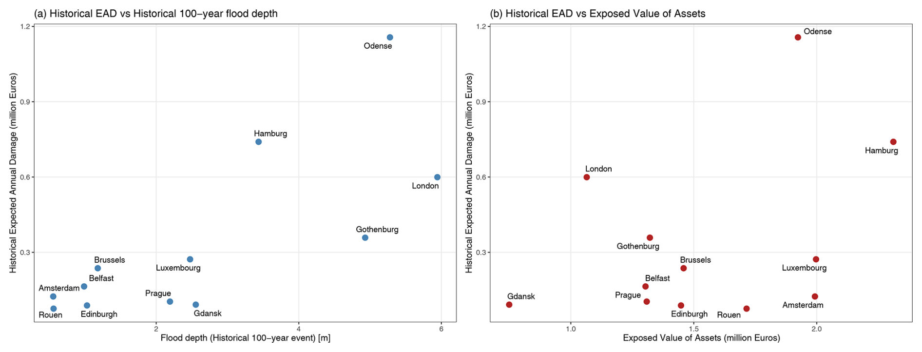
Figure 11 A comparison of the driving components of the flood EAD in each of the 12 city grid cells: (a) relates the historical ensemble mean EAD to the historical 100-year flood depth (hazard), and (b) relates the historical ensemble mean EAD to the exposed value of assets (exposure).

In Fig. 10a the climate model ensemble spread (total length of the box plots) indicates the uncertainty across the climate model simulations. As expected, uncertainty in EAD is greater for the future period, reflecting the increasing divergence among climate ensemble projections over time within this perturbed parameter ensemble. This rise in uncertainty varies by location, with Gothenburg and Luxembourg grid cells showing particularly pronounced future uncertainty. Further investigation is required to understand the drivers of these differences in climate model uncertainty across locations.

3.2 Exploring risk in synthetic portfolios

Historical and projected future estimates of idealised flood risk, derived from the 12-member UKCP18 RCM ensemble, are integrated with various representations of synthetic pension portfolios (as outlined in Sect. 2.3) to enhance sector-specific realism and relevance.

Figure 12 compares the total EAD of two synthetic pension portfolios. The two portfolios are similar in many ways: each portfolio comprises 450 sampled locations and has an estimated combined economic value of approximately EUR 0.89 billion, based on the asset value exposure metric used in the analysis (shown in Fig. 8c). Indeed, visually, the spatial distribution and variability of asset locations appear very similar. However, their total EAD differs substantially, with Portfolio 2 exhibiting significantly higher values than Portfolio 1 in both historical and future periods. This arises primarily because Portfolio 1 and Portfolio 2 are sampled such that 20 % and 80 % of locations are at risk of flooding respectively (where locations at risk of flooding are indicated by non-zero flood depth for events up to at least the 1-in-75-year return-period in the CEMS flood hazard maps, see the left panel of Fig. 6).

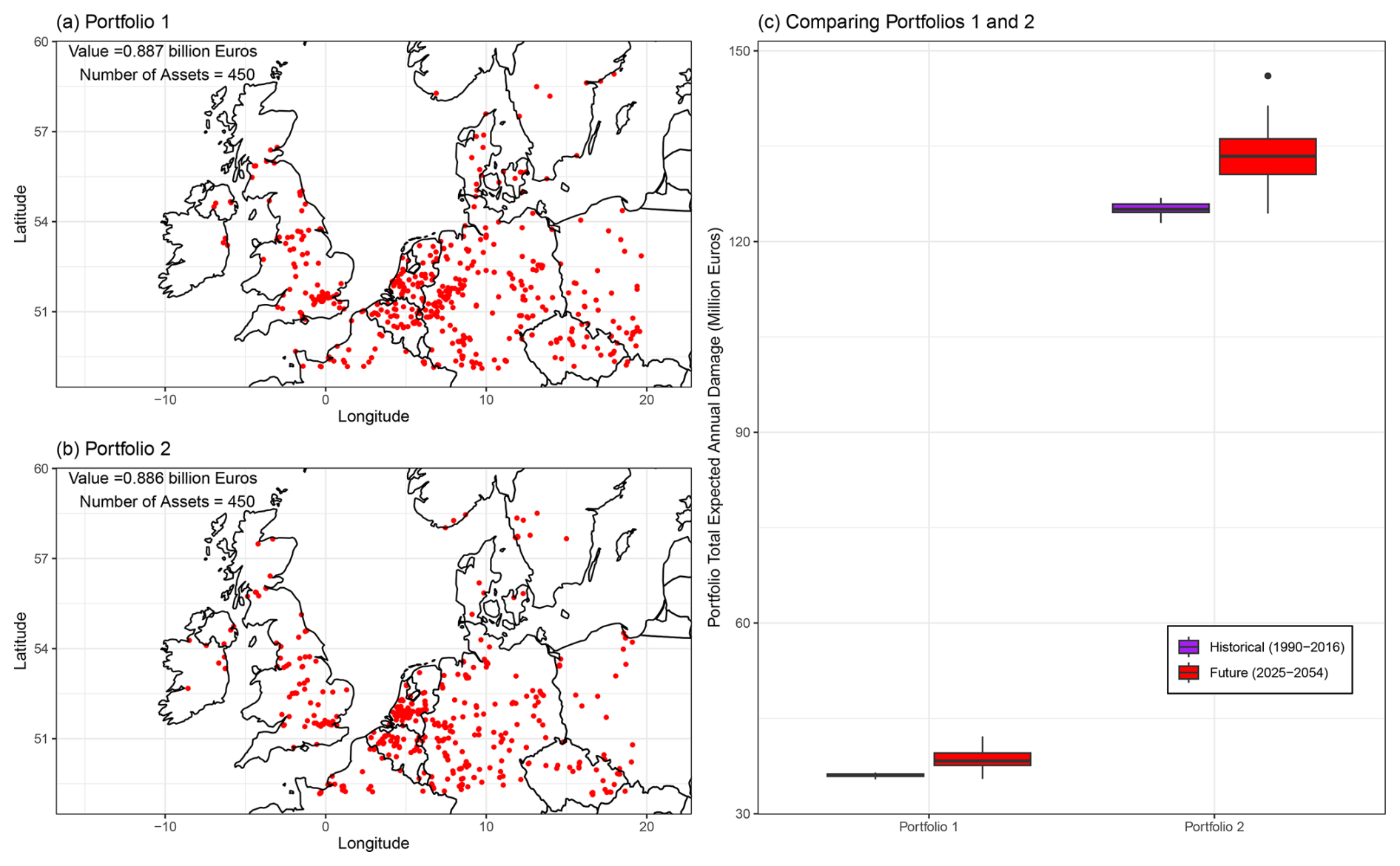
Figure 12 A demonstration of the difference in idealised flood risk between two synthetic pension portfolios: (a) Portfolio 1: the geographical locations of 450 randomly sampled locations used to represent a synthetic pension portfolio of 450 assets, such that 20 % of the locations are at-risk of flooding (blue points in the left panel of Fig. 6), (b) Portfolio 2: as in panel (a) but such that 80 % of the locations are at-risk of flooding, (c) box-plots comparing the portfolio total EAD for Portfolios 1 and 2, in both the historical and future periods. The uncertainty in the box-plots quantifies the UKCP18 RCM ensemble spread, where box, whiskers and outliers as defined in Fig. 10. In panels (a) and (b) the total value of the portfolio asset locations is given in the top left corner, estimated using the exposure metric of total value of assets in Fig. 8c.

This example highlights the critical need for pension sector asset managers to quantify the physical climate risks embedded within their portfolios. Portfolios that appear broadly similar based on aggregate characteristics may nevertheless have materially different risk profiles, and these differences are not always evident without explicit risk analysis. Accurately assessing this risk is therefore essential, and, where feasible, proactive adaptation measures should be implemented to reduce exposure and vulnerability.

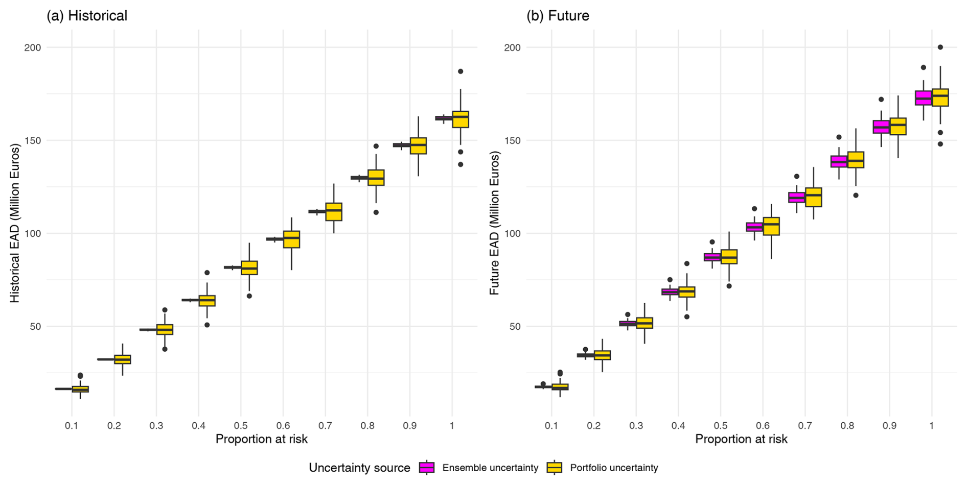
Figure 13 Comparison of uncertainty in estimated flood risk (Expected Annual Damage, EAD) arising from portfolio composition and climate model ensemble members. Boxplots show EAD as a function of the proportion of portfolio locations at risk of flooding (0.1–1 in increments of 0.1). For each proportion at risk, the distribution in yellow represents variability across 100 synthetic portfolios (portfolio uncertainty), where EAD is first averaged over the 12 UKCP18 RCM ensemble members for each portfolio. The distribution in magenta represents variability across the 12 ensemble members (ensemble uncertainty), where EAD is first averaged over the 100 portfolios for each ensemble member. This is shown for (a) Historical climate EAD and (b) Future climate EAD. In both panels, EAD is calculated using the same underlying portfolios and ensemble members, enabling a direct comparison of the relative contributions of portfolio and climate uncertainty.

A deeper analysis of how varying the proportion of at-risk locations influences overall risk is presented in Fig. 13, which shows how historical and future EAD varies across 100 synthetic portfolios as a function of the proportion of assets at risk. The boxplots summarise variability arising from both portfolio composition and climate ensemble members, with EAD averaged over the alternate dimension in each case.

Figure 13 shows that EAD increases systematically with the proportion of at-risk locations in both the historical and future periods, highlighting the strong dependence of risk on portfolio exposure. In particular, portfolios with low (e.g., 20 %) and high (e.g., 80 %) proportions of at-risk assets exhibit clearly separated EAD distributions, indicating that the proportion at risk provides a useful first-order proxy for EAD. However, there remains a substantial spread in EAD values within each exposure level, such that portfolios with the same proportion of at-risk assets can still experience markedly different levels of damage. This demonstrates that, while the proportion at risk captures a large component of flood risk, it is not sufficient on its own to fully explain differences in EAD, and additional factors such as asset value distribution and spatial configuration also play an important role.

Both panels in Fig. 13 clearly show that the variability in EAD associated with portfolio composition is substantially greater than that arising from the UKCP18 RCM ensemble. For each proportion of assets at risk, the spread of the yellow boxplots (portfolio uncertainty, where EAD is averaged across ensemble members) is consistently much larger than that of the magenta boxplots (ensemble uncertainty, where EAD is averaged across portfolios). This demonstrates that the spatial distribution and value of assets within a portfolio exert a stronger influence on EAD than the specific climate realisation (ensemble member) used to represent extreme rainfall.

Nevertheless, the magenta boxplots indicate a non-negligible spread across ensemble members, particularly at higher proportions of at-risk assets, showing that climate uncertainty still contributes to variation in EAD. Furthermore, the increase in EAD with proportion at risk is evident in both panels, with higher-risk portfolios exhibiting larger absolute variability. Comparing panels (a) and (b) in Fig. 13, the overall spread across ensemble members increases in the future period, suggesting that EAD estimates become increasingly sensitive to the choice of ensemble member as the analysis period approaches the middle of the century.

Taken together, these results highlight that while portfolio composition is currently the dominant driver of variability in estimated flood risk, uncertainty due to climate projections becomes increasingly important as risk levels increase and into the future. This reinforces the need for portfolio-specific risk assessments, as both the proportion and spatial distribution of exposed assets strongly influence estimated impacts and their associated uncertainties.

4 Exploring adaptation

Climate adaptation refers to the process of adjusting natural and human systems to minimise harm associated with climate change. It involves implementing strategies such as improving infrastructure resilience, developing drought-resistant crops, enhancing flood defences, and revising policies to cope with changing conditions.

The results in Sect. 3.1 and 3.2 highlight how physical climate risk from extreme rainfall is a concern for commercial property assets in the current climate and increases in future climate. To reduce this risk and build resilience, the pension sector must invest in climate adaptation.

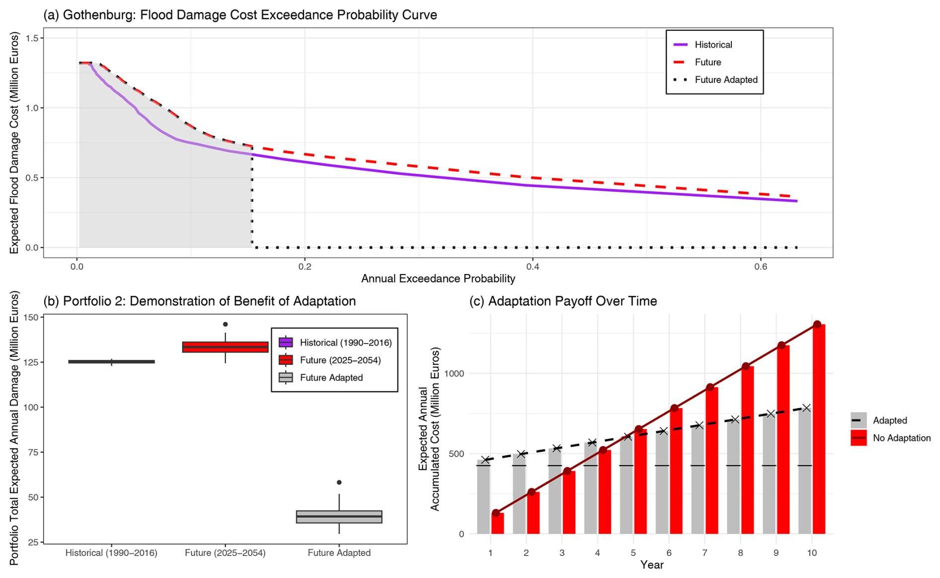
Figure 14 An illustration of the potential benefits of climate adaptation within the pension sector using a toy example associated with synthetic Portfolio 2 (introduced in the previous section). (a) Flood damage cost annual exceedance probability (AEP) curve for a grid cell in the centre of Gothenburg for the historical period (1990–2016), future non-adapted scenario (2025–2054), and future adapted scenario. The grey shaded area represents the Expected Annual Damage (EAD) after adaptation. AEP is defined using the Poisson representation (see Sect. 2.5), such that the maximum AEP corresponding to a 1-year return-period is approximately 0.63. Values beyond this (i.e. return-periods shorter than 1 year) are not shown. (b) Portfolio-level EAD comparison for historical, future, and future adapted scenarios, illustrating the reduction in risk due to adaptation. The uncertainty in the box-plots quantifies the UKCP18 RCM ensemble spread, which box, whiskers and outliers are as defined in Fig. 10. (c) Adaptation payoff over time: cumulative damage costs for adapted assets (grey bars) versus no adaptation (red bars), with dashed and solid lines indicating cumulative totals. The horizontal black lines on the grey bars show how much of the accumulated cost in the future adapted scenario is due to the cost of adaptation (rather than the loss due to flood risk).

To illustrate the potential benefits of climate adaptation within the pension sector, we suppose that all asset locations in Portfolio 2 (Sect. 3.2) are adapted to withstand flood depths up to and including the historical 1-in-10-year event (e.g. through the building of flood defences). This adaptation effectively truncates the upper tail of the future annual exceedance probability (AEP) curve at the relevant annual exceedance probability. The future Expected Annual Damage (EAD) at each location is then calculated as the area under this truncated curve. Figure 14a demonstrates this for a grid cell in the centre of Gothenburg, where the historical 1-in-10-year flood depth aligns with the future 1-in-6-year event. Consequently, the adapted AEP curve is truncated so that flood damage costs are zero for exceedance probabilities greater than $\mathrm{1}-\exp (-\mathrm{1}/\mathrm{6})$ (see Sect. 2.5). The grey shaded region then represents the future adapted EAD at this location.

This approach is applied to all locations in Portfolio 2. It is important to note that this conversion is calculated separately for each location and ensemble member based on their respective return-level curves. As a result, the equivalent future return-period corresponding to the historical 1-in-10-year event varies across both space and ensemble members. Figure 14b compares the portfolio total EAD before and after this adaptation is implemented for the future period. This toy demonstration shows how adaptation results in a large reduction in the EAD and hence physical risk associated with the pension portfolio, highlighting the important role adaptation could have.

Such adaptation measures may be costly and hence their implementation may not seem financially beneficial when first considered. However, it is likely that such costs would be quickly recouped over a relatively short period due to the significant reduction in future losses. To explore this, the cumulative cost of a given portfolio can be estimated over time and scenarios with and without adaptation measures in place can be compared.

To illustrate this, we use the same toy example and assume that adapting Portfolio 2 assets to withstand the historical 1-in-10-year flood depth incurs a cost of EUR 500 per m² for 1 m of flood depth. This assumption is informed by European cost estimates synthesised by Aerts (2018), which suggest that wet and dry flood-proofing measures for approximately 1 m of flood depth correspond to costs of order EUR 100–350 per m² for residential buildings. Given the focus of this study is on non-residential assets, and recognising the additional service complexity and higher specification typically required for such buildings, we adopt an upper-bound value of EUR 500 per m² for 1 m of flood depth. This choice is intended to provide a precautionary assumption suitable for illustrative adaptation analysis, rather than site-specific appraisal.

For Portfolio 2, this corresponds to an adaptation investment of approximately EUR 400 million. Figure 14c compares the cumulative annual cost for Portfolio 2 under two scenarios: with and without adaptation. In the no-adaptation case (red bars), the ensemble mean EAD for the future period, around EUR 130 million per year (see Fig. 14b), is accrued annually. In contrast, the adaptation scenario involves the substantial upfront adaptation cost in year 1, followed by a much lower EAD of approximately EUR 36 million per year. Because the adapted EAD is significantly reduced, the cumulative cost of the adapted scenario becomes lower than the non-adapted scenario by year 5, despite the initial investment. This demonstrates that adaptation can deliver a strong financial return within a relatively short time frame, reinforcing its role as a cost-effective strategy for managing climate-related risks in the finance sector. We note that the EAD represents an average annualised risk metric and does not incorporate discounting. Incorporation of discount rates would be required for formal cost–benefit analysis of adaptation measures, but this is beyond the scope of the present study and would require context-specific assumptions regarding time horizons and economic parameters.

We emphasise that this representation of adaptation is intentionally simplified and serves as an illustrative example within the modelling framework. In particular, the approach assumes uniform protection of assets up to a specified return-level, does not account for defence failure, spatial heterogeneity in vulnerability or protection standards, or the phased implementation of adaptation over time. In addition, the adaptation cost model is highly idealised and does not capture site-specific engineering, economic, or policy constraints. As such, the results should be interpreted as indicative of the potential scale and implications of adaptation, rather than as a detailed or decision-ready assessment.

5 Limitations

Throughout the paper we have alluded to limitations in the method, and for clarity we provide a clear overview of the key caveats here.

5.1 Assumption of stationarity within time periods

The assumption of stationarity within each time period (historical and future) in the rainfall EVA model may mask potential within-period non-stationarity, particularly given the concentration of recent losses. However, exploratory analysis including a temporal covariate did not indicate a clear monotonic trend, instead suggesting variability dominated by internal climate variability. Future work could investigate covariate-based approaches to better separate externally forced trends from internal variability.

5.2 Assumption of stationarity in the rainfall–flood relationship

The methodology assumes that the statistical relationship between rainfall extremes and flood depth remains stationary across historical and future climate periods. In reality, climate change may alter hydrological processes such as runoff generation, soil moisture dynamics, drainage efficiency, and flood routing, potentially modifying the rainfall–flood relationship over time. These effects are not explicitly represented in the present framework. As a result, projected changes in flood hazard reflect changes in rainfall extremes rather than potential changes in catchment response. This assumption is appropriate for the large-scale, illustrative analysis undertaken here, but would need to be revisited in applications intended for asset-scale flood risk assessment.

5.3 Simplified rainfall–flood mapping and lack of hydrological modelling

Limited availability of consistent, open hydrological modelling data at continental scale necessitates the use of a simplified statistical mapping between rainfall extremes and flood depth. In some locations, flood models now exist that can provide flood risk information at very high resolution over limited regional domains (e.g. for the UK, at up to 20–25 m resolution) however, important details of methods and data used for flood risk estimates may not be in the public domain (Bates et al., 2023). Our simplified statistical mapping approach replaces a physically based modelling chain, and therefore cannot represent key processes such as runoff generation, antecedent soil moisture, flow routing, floodplain dynamics, and the influence of flood defences. In particular, the mapping between rainfall and flood hazard is implemented as a quantile-to-quantile relationship. This does not reflect the full convolution of rainfall variability with catchment processes, whereby multiple rainfall events can lead to similar flood responses. As such, the method provides only a first-order approximation to the underlying flood hazard distribution. Critically, our simplified rainfall–flood relationship is not explicitly validated against observed flood events or independent hydrological model output. A further limitation arises from the mismatch in spatial resolution between datasets. Rainfall extremes are modelled at 12 km resolution, while flood depths are represented at 100 m resolution. The mapping therefore assumes that rainfall statistics at the climate model scale are representative of local flood-generating conditions. As a result of these various limitations, there is substantial structural uncertainty in the resulting flood depth estimates, particularly in their absolute magnitude. Consequently, the risk estimates presented in this study should not be interpreted as location-specific or decision-grade assessments, but rather as illustrative estimates intended to demonstrate methodology and explore relative changes and sensitivities. Despite these limitations, the approach retains value by providing a transparent and internally consistent means of linking changes in rainfall extremes to corresponding changes in flood hazard at large spatial scales, where use of high-resolution physically based hydrological modelling is not feasible using currently available open data.

5.4 Limitations around flood modelling information used

We use flood maps for a limited number of return-periods that are available publicly for the present day only. Flood extent and depths may increase under more intense and/or frequent rainfall unless adaptation measures are implemented (e.g. Alfieri et al., 2016), and so this may result in an underestimate of risk in the future as more properties may be exposed to flooding. Users should also be aware of potential limitations around the flood modelling framework for the flood maps that are publicly available, such as the absence of flood protections and rivers with an upstream area below 500 km² as well as the model representation of river channels and the topography of lowland areas (Dottori et al., 2022). In addition, these flood maps represent river flooding only. Surface-water (pluvial) flooding driven by intense local rainfall is not captured, and therefore some flood pathways and hazard intensities may be underestimated in areas where surface-water processes dominate.

5.5 Limited range of plausible rainfall extremes

For our demonstration purposes we use one climate model with one driving scenario, with 12 ensemble members. These simulations are widely used for risk assessment in the UK context (Mittal et al., 2025), and the nature of the perturbed parameter ensemble provides a spread of uncertainty. To provide coverage across Europe we use data from a regional climate model, rather than a convective-permitting model. Convective-permitting models have been shown to improve the representation of extreme rainfall events and to project more intense extreme downpours in the future (e.g. Kendon et al., 2014, 2023). However, for these models to operate at high resolution, domains are typically limited to a small area (e.g. country-scale) or a short timespan, hindering climate-timescale analysis (over 30 years) across a continental area. Regarding the use of a single climate scenario (here RCP8.5), for the near- to mid-century period considered in this study (2025–2054), differences in projected warming between emissions scenarios remain relatively small, with more pronounced divergence emerging primarily after around 2050 (see Fig. 1 in Met Office, 2018). Under intermediate emissions scenarios (e.g. RCP4.5 or RCP6.0), projected changes during this period would be expected to follow broadly similar spatial patterns to those under RCP8.5, with differences in magnitude becoming increasingly pronounced later in the century. As a result, the use of a single high-emissions scenario enables a clear and internally consistent illustration of the methodology without materially affecting the qualitative conclusions regarding relative patterns of rainfall extremes and flood risk. Future work, particularly for more distant time horizons, could extend this analysis to multiple emissions scenarios as suitable high-resolution pan-European climate datasets become available, enabling a more explicit assessment of scenario-dependent uncertainty.

5.6 Assumptions around synthetic portfolio design and financial context

For this initial work, we have randomly dispersed commercial properties to create synthetic (invented) but plausible portfolios of one class of assets. We have also created idealised scenarios where we artificially force portfolios to exist mostly, or not, on flood plains. This is highly idealised, but suitable for demonstration purposes to illustrate differences between portfolios. Sakai and Yao (2023) analyse damages from flood events in the UK to small-medium size enterprises, highlighting the differences in financial impact across sectors and sizes of portfolios. The complexity of damages further motivates the need to assess risk on a case-by-case basis for portfolios. Sakai and Yao (2023) highlight the importance of the losses-to-turnover ratio for negative financial impact; we have not implemented an estimate of losses from turnover into this assessment but note that this is a necessary area for development for a comprehensive financial risk assessment. In addition, the methodology is not validated against observed economic losses, insurance claims, or official flood risk products; given the differences in spatial scale, temporal aggregation, and modelling assumptions, such comparisons are not directly comparable, and the resulting damage estimates should therefore be interpreted as indicative rather than calibrated values. In future potential revisions to this framework, using physically based hydrological and hydrodynamic modelling, such validation against observed impacts and official risk products would be essential to ensure the reliability and applicability of the results.

5.7 Use of a generic vulnerability function

In this idealised example we have used the same vulnerability function to relate the flood depth to asset fraction of damage for all assets/locations. While this approach provides a useful baseline, future work and real-world applications would benefit from incorporating asset-specific vulnerability profiles. This also illustrates the need for more detailed information on properties, such as might be obtained by mandating flood property certificates and regularly updated information on flood protection measures.

5.8 Use of national average exposure values

Exposure is represented using national average non-residential property values per unit area. This approach ignores potentially large intra-urban and regional variations in asset values driven by land use, economic activity, and urban structure. As a result, estimated damages at individual locations may be over- or under-estimated in absolute terms. Incorporating higher-resolution exposure data would be an important extension where suitable open-source datasets become available.

5.9 Lack of uncertainty and sensitivity analysis

Risk assessments inherently require modellers to make a series of subjective decisions about how each component of risk is represented, including the choice of datasets and the methods used to characterise hazard, exposure, and vulnerability. Consequently, when applying this risk assessment process in a less idealised context, it is important to explore alternative methodological options in order to assess the sensitivity of the results and to quantify uncertainty arising from these input data and modelling assumptions. Examples of such approaches are provided in Dawkins et al. (2023b) and Babich Morrow et al. (2025).

6 Societal implications

The method we present here is pragmatic, with several important caveats and limitations. In particular, the simplified and unvalidated mapping between rainfall and flood hazard means that the outputs should be interpreted as indicative rather than precise estimates of asset-level risk. Our aim is to raise awareness and help stimulate closer assessment of physical climate risk, and ultimately help lead to climate-informed decision making, rather than provide a particular risk assessment for a particular asset or set of assets. This demonstration may also help stimulate commission of climate services tailored to bespoke portfolios using state-of-the-art tools and data, which could include, where available, the purchase of hydrological modelling data for asset locations from a flood modelling firm. With hydrological modelling data in a particular area, future work using similar synthetic portfolio experiments can also be performed to demonstrate the potentially diverse risks that different European portfolios may experience from extreme rainfall under near term climate change.

The method we present here is pragmatic, with several important caveats and limitations, however we aim to provide useful and usable methods using currently available data for demonstration purposes. These limitations should be carefully considered and we suggest our method be supplemented with additional information where available for any use case of a particular portfolio. However we present our method as a way to produce spatially explicit and financially meaningful illustrative flood risk estimates to help drive change in financial investments (e.g. pension funds) or in other industry settings where climate risk is not already considered for property assets.

7 Conclusions

This study presents a transparent and pragmatic framework for assessing physical climate risk from extreme rainfall for European portfolios of property assets using openly available data and methods. By integrating hazard, exposure, and vulnerability components, we provide illustrative estimates of Expected Annual Damage for both historical and near-future climates.

The analysis highlights four key insights:

• Current and future risk is substantial. Pension portfolios comprised of property assets may already face notable flood-related financial risk, with this risk likely to increase across Europe under near-term climate change.

• Portfolio composition matters. Differences in asset location and hence value at-risk of flooding drive greater variability in risk than climate model uncertainty within this framework.

• There is a need for improved risk information in decision-making. Financial actors (such as asset managers of pension funds) would benefit from incorporating physical climate risk considerations to support long-term financial resilience.

• Climate adaptation reduces risk. Adaptation measures have the potential to substantially reduce EAD and improve financial outcomes, although the magnitude of these benefits is dependent on the simplified assumptions adopted here.

While the approach is designed for demonstration and awareness-raising, it highlights the value of developing transparent and interpretable tools for assessing physical climate risk in the financial sector. A key limitation of the approach is the use of a simplified and unvalidated mapping between rainfall extremes and flood hazard, constraining the realism and applicability of the results for decision-making. Future work should refine the hazard modelling, expand climate scenarios, and incorporate asset-specific vulnerability profiles to enable more comprehensive and decision-relevant risk assessments. Ultimately, integrating climate-informed perspectives into investment planning is likely to be important for improving the resilience of financial systems in a changing climate.