Investigating metamodeling capability to predict sea levels and marine flooding maps for early-warning systems: application on the Arcachon Lagoon (France)

Marine flooding events during storms are expected to occur more frequently due to sea level rise. Hence, early warning systems (EWS) dedicated to marine flooding are expected to develop in the coming years. In this study, we compare three data-driven methodologies to overcome the computational burden of numerical simulations. They are all based on the statistical analysis of pre-calculated databases, to downscale total water levels and to predict marine flooding maps from offshore metocean operational forecasts. While the first one is a simple analog-based research from offshore metocean conditions, the next two both use a machine learning type metamodel to predict total water levels at the coast, and either an analog or a deep-learning approach to predict marine flooding maps. The analysis, carried out with a cross-validation exercise and historical storms on the pilot site of Arcachon lagoon (Southwest of France), reveals that the analog-based approach is a valuable first step to explore the dataset and improve the understanding of flooding phenomena, but lack precision for operational forecast applications. On the other hand, the two metamodel-based approaches are more suitable for fast prediction with a lower prediction error of inland water heights for the deep-learning approach (on the order of 10 cm). Both approaches can then be complementary depending on the type of event, the required level of prediction accuracy to support operational decision making, and the forecast lead time. In this sense, the study also underlines the usefulness of precalculated databases to conduct a preparatory work with crisis managers to determine the type of information and the right level of complexity required to address operational needs.

1 Introduction

The high rates of population growth and urbanization in coastal regions tend to constantly increase marine flooding risks in low-lying areas. Projections estimate the number of people living in coastal flood-prone areas at more than 200 million by 2100 (Hauer et al., 2021). Marine flooding is a phenomenon resulting from the combination between various processes generated at different time and space scales (atmospheric circulation, waves, atmospheric surge, tide, and sometimes river discharge) and the local configuration of the coast (coastal bathymetry and elevation, protection structures, land use, hydraulic networks, etc.). The numerous variables, scales and sources of uncertainty make marine flooding events very complex to predict several hours or days in advance. However, marine conditions forecasts (Toledano et al., 2022; Lorente et al., 2019) and coastal flood early warning systems (Stansby et al., 2013; Dietrich et al., 2013; Irazoqui Apecechea et al., 2023) have gained a significant impulse in the last decades. Today, there is a growing demand not only to shift towards ever more local marine flooding forecasts, but also to better account for uncertainties, which requires approaches using multi-sources or even probabilistic metocean conditions (see a recent discussion by Turner et al., 2024).

Recent improvements in high performance computing enabled numerical weather prediction systems to move from deterministic to probabilistic forecasting using Ensemble Prediction Systems (EPS) (Descamps et al., 2015). While EPS are increasingly used to predict river flows and induced continental floods in several countries (Wu et al., 2020), it is only emerging for marine flooding (Lecacheux et al., 2018: Biolchi et al., 2022). Despite ongoing efforts to develop new generations of high performance oceanographic and phase-resolving models accounting for complex processes (Filippini et al., 2024), the main challenge still remains the computer power required to run multiple simulations with a chain of models of increasing resolutions (from a hundred meters for coastal waves and surges to a few meters for marine flooding). Most of the examples of – deterministic or probabilistic – systems forecasting explicitly marine flooding rely on three solutions to overcome these limitations: (1) High Performance Computing (HPC); (2) reduced process complexity with generalized overflowing models or empirical formula; and (3) statistical analysis of pre-calculated flooding scenarios (Lecacheux et al., 2018; Beuzen et al., 2019). Now, operational needs and constraints of potential users must guide these technical choices. It is about linking top-down and bottom-up approaches by connecting technical capabilities with local users' needs to identify the suitable level of complexity able to produce the right level of information (parameters, resolution, and precision) for decision making (Demeritt et al., 2016).

In this study, we focus on methodologies based on pre-calculated databases to downscale total water levels (TWL) and marine flooding maps from offshore metocean conditions as developed at European scale in ECFAS project (Le Gal et al., 2023, 2024). Databases are often used to work by analogy, based on storm similarity with forecasted conditions, but this solution also provides complementary possibilities to (1) improve the understanding of marine flooding processes and identify key scenarios and action plans to facilitate foresight and anticipation in crisis management (Luesink et al., 2024); (2) apply machine learning (denoted ML) type methods to develop very rapid forecasting models (or metamodels) able to replace numerical models to carry out simulations in real time. ML-based metamodeling techniques have made great progresses in this field of application (ML-based metamodeling techniques have made great progresses for flood predictions (storm surge: e.g., Macdonald et al., 2025; hurricane: e.g., Irwin et al., 2025; tsunami: e.g., Ragu Ramalingam et al., 2025; estuarine: e.g., Wang et al., 2025a; river flood: e.g., Wang et al., 2025b) and opens up encouraging perspectives for marine flooding forecasting. Through a statistical analysis of pre-calculated training databases, they can predict key flooding indicators (surge, discharge, water height on land, etc.) at a given spatial location of interest within reasonable time and computing resources while preserving the accuracy of full process models. Yet, some issues remain to push this metamodel-based approach toward operational applications, and more specifically the production of spatialized indicators such as inland water height maps, which is still a matter of active research research (among others, Ma et al., 2022; Spiller et al., 2023; Fraehr et al., 2024; Rohmer et al., 2024a; Jung et al., 2025). Indeed, producing such spatialized indicators requires to overcome the difficulty in learning complex mathematical relationships between the metocean forcing conditions and the generation of flood maps (i.e. output of high dimensional related to the number of pixels, typically of several 10 000 s).

The objective of this work is to investigate different approaches, based on pre-calculated databases, to produce information that is relevant for operational forecast applications. This implies analysing not only the added value in terms of accuracy regarding the required implementation effort but also in terms of adequacy according to the needs of crisis managers. We consider three approaches with increasing complexity. The first one is a simple analog-based method, which is based on the analysis of the similarity between the coming metocean conditions and an individual event in the pre-calculated training database (also named as “look-up table”). The next two are ML-based methods aiming to supplement or substitute the analog-based approach with (1) a regression-type metamodel to predict total water levels in the lagoon; (2) deep learning techniques to predict the marine flooding maps. To support the analysis, we focus on the Arcachon lagoon (Southwest of France, Fig. 1) where a database of a few hundred flood scenarios have been simulated for the Service of Civil Defense in a previous study (Lecacheux et al., 2023) and a participatory work with crisis managers enabled to identify operational needs and critical thresholds associated with graduated categories of flood impacts.

In the following chapters, we present the pilot site, the databases and lessons learnt from their analysis with crisis managers in Sect. 2, the three approaches for total water levels and marine flooding prediction in Sect. 3, and the comparison of their skills in Sect. 4. In the discussion in Sect. 5, we analyze the pros and cons of the different methods regarding local users' needs while Sect. 6 summarizes the main conclusions and addresses the perspectives for application of these models for operational forecast.

2 Site, databases setup and analysis

2.1 Study area

Arcachon lagoon is a large low-lying area located in a semi-closed environment and mainly subject to marine overflows driven by offshore storm surge and wave forcing associated with local winds (Fig. 1A). It is a well-studied site, which benefits from a rich bibliography, covering both its general functioning (Bouchet et al., 1997a), the geological and morphosedimentary context (Saltel et al., 2014), the hydrological functioning (Bouchet et al., 1997b) and oceanographic characteristics (Castelle et al., 2007; Dupuis et al., 2006). In recent years the lagoon has been regularly affected by minor to moderate marine flooding notably during storms Klaus (2009), Xynthia (2010), and more recently Céline (2023). As illustrated on Fig. 1B, these storms generated total water levels (tide + storm surge) from annual (∼3 m NGF, NGF being the official vertical reference system to measure elevations in France) to approximately 10 years (∼3.5 m NGF) return periods at the Arcachon-Eyrac tide gauge but there is no historical example of event beyond. Yet, statistical and hazard studies (Mugica et al., 2014; SHOM, 2022) demonstrated that a 100 year return period event could reach up to 3.7 NGF at the same location, then affecting almost ten thousand of persons (SIBA, 2015).

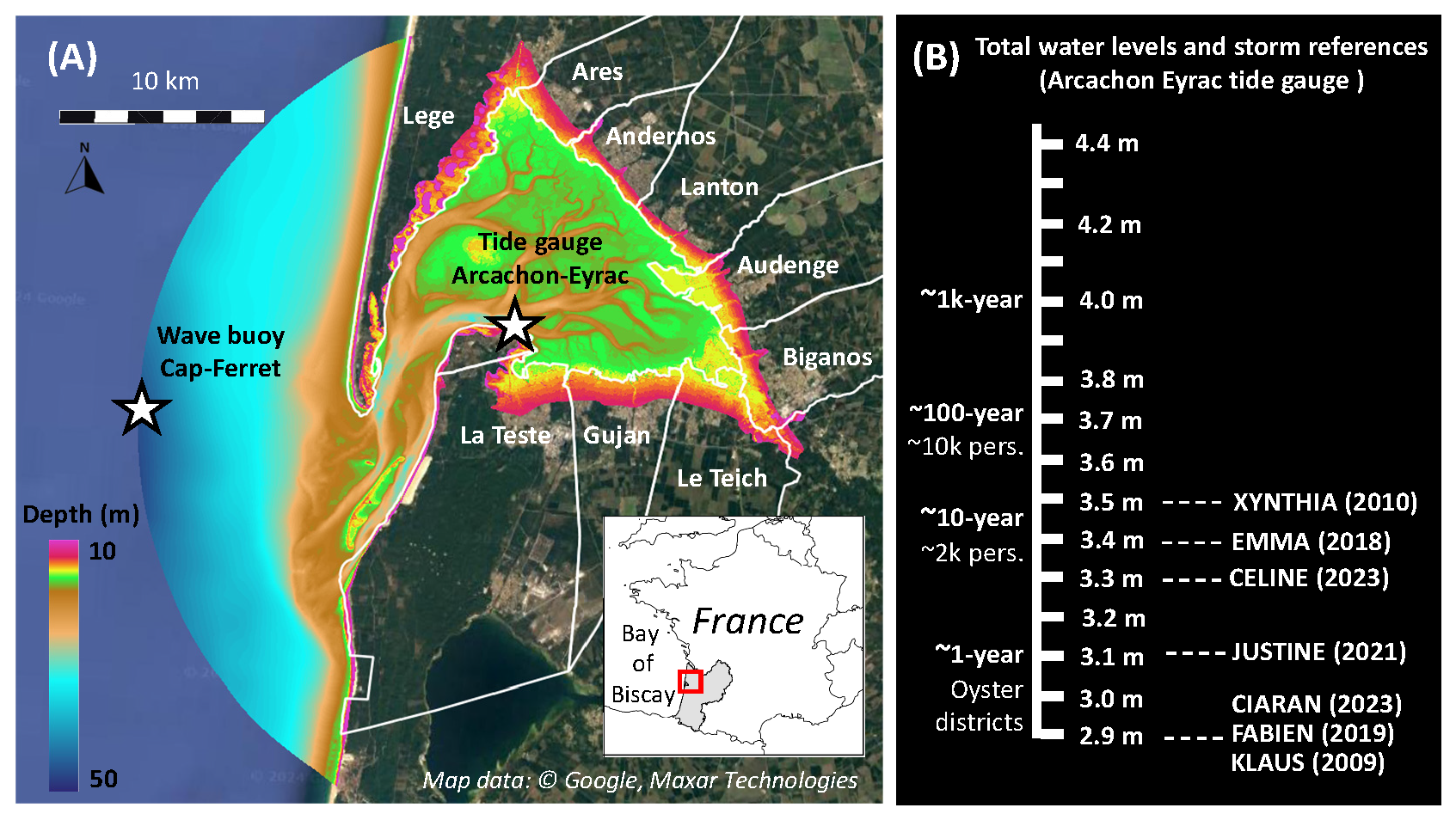
Figure 1 (A) Location and bathymetric map of the study site: white stars indicate the location of the tide gauge named Arcachon-Eyrac and the wave buoy named Cap-Ferret. (B) Total Water levels (m NGF) with associated return periods and historical storms references. Map data: © Google, Maxar Technologies.

Based on this bibliography and historical events, the main elements to consider when modeling coastal floods on this area are

• Marine flooding by overflowing is dominant on the scale of the entire lagoon even if local sectors can also be exposed to wave overtopping (as the seafront of Andernos, see location in Fig. 1A).

• Waves have a significant effect on marine flooding through the generation of a homogeneous wave setup inside the lagoon (up to several tens of centimeters) generated by the breaking of the swell at entrance of the lagoon).

• West/northwest winds are the most frequent and can generate an additional storm surge inside the lagoon particularly at the extreme east (from Biganos to Arès) where total water levels may reach several tens of centimeters higher than in Arcachon in case of strong winds;

• Although river floods are characteristic hazards of wetlands such as the Arcachon lagoon, available studies and measures do not enable to characterize the conjunction between storm surge and river floods on this site (in particular at the Leyre delta between Le Teich and Biganos).

In this study we focus on marine overflowing only, without considering neither wave overtopping (localized on the seafront of Andernos) nor the conjunctions of river flood and storm surge (located in the Leyre Delta). Thus, the study focuses on the simulation of the total still water level or TWL (including tide, atmospheric surge caused by winds and pressure drop and the wave set-up caused by the breaking of waves in entry of the lagoon) and the resulting coastal flooding. The dynamic water level (including the swash component) is not taken into account.

2.2 Design of scenarios for learning and validation of the metamodels

The synthetic storm conditions constituting the scenarios of the pre-calculated database (used for the analysis of the physical processes and for setting up the ML-based techniques, see Sect. 3) are built on the basis of a tri-variate statistical analysis of the extremes of wind, wave and surge conditions at the Cap-Ferret wave buoy located at a depth of 50 m in front of the lagoon (Fig. 2A). The reference data are extracted at high tide from reanalyses over the period 1979–2009: CFSR (Saha et al., 2010) for wind, ANEMOC 3 (Raoult et al., 2018) for waves and MARS30 (Mugica et al., 2014) for the storm surge. After fitting probability laws for significant wave heights (Hs), skew surge (SPM, defined as the difference between the maximum simulated water level and the predicted high tide level) and wind intensity (U) using the Generalized Pareto law (Coles et al., 2001), the dependence models are adjusted for U, Hs and SPM according to the conditional extreme model of Heffernan and Tawn (2004) while managing the covariates (peak period – Tp, wave directions – Dp and winds – Du). Finally, many random combinations (here chosen at 150 000) with the same statistical characteristics as the input data are generated via Monte Carlo simulations. To constitute the learning database, 50 moderate to strong storm conditions (Hs>4 m) are selected via a clustering algorithm (Camus et al., 2011) aimed at maximizing the diversity of scenarios (Fig. 2A). These 50 conditions are associated with 10 tide levels between coefficients 40 and 120 (i.e. varying from 1–2.8 m NGF at the tide gauge every 20 cm), bringing the total number of scenarios to 500. Each scenario is therefore described by 6 storm parameters at the buoy (U, Du, Hs, Tp, Dp, SPM) and a high tide level (T) at the gauge.

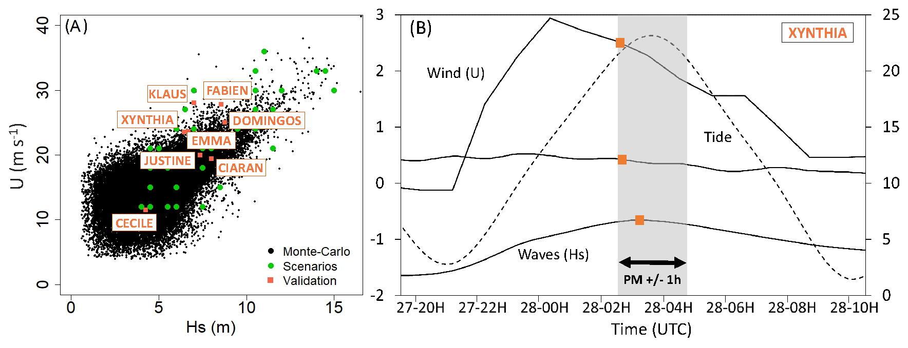
Figure 2 (A) Monte-Carlo simulations (black points), synthetic (green points) and historical or validation (orange points) storm conditions at high tide. (B) Example of storm parameters time series and extraction of conditions at high tide (orange points) for storm Xynthia (2010).

These synthetic events are completed with historical and pseudo-historical events for validation and demonstration purposes. Historical events (Table 1) correspond to 8 storms (Klaus, Xynthia, Emma, Fabien, Justine, Ciaran, Domingos, Céline) that occurred between 2009 and 2023 and whose forcing conditions are extracted from observed winds and waves as well as reanalysed storm surge (from Météo-France Arpège model) at the Cap-Ferret wave buoy location. Table 1 and Fig. 2A show their characteristics at high tide and Fig. 2B an example of parameters time series for storm Xynthia. Although they are well scattered in the synthetic dataset range, these events remained quite limited in terms of total water level (Fig. 1B) and marine flooding impact (as mentioned in Sect. 2.1) because the most intense storms (Fabien, Klaus and Domingos) occurred at low tide coefficients. Thus, pseudo-historical events are added by combining these 8 storms (described by parameters U, Du, Hs, Tp, Dp, SPM) with the same ten high tide levels (T) as the synthetic events, to create marine flooding events of different severity (greater or lower than historical events). This results in 80 additional events hereafter named Pseudo_StormName_TideLevel(NGF).

Table 1 Storm parameters (U, Du, Hs, Tp, Dp, SPM) at high tide for the 8 historical storms.

2.3 Flood numerical model set up and simulation of the scenarios

The marine flooding model set up for the project includes a chaining of WW3 spectral wave model (Tolman, 2014) and UHAINA hydrodynamic models (Filippini et al., 2024) that resolves Saint-Venant equations. The grid is an unstructured mesh with a resolution from kilometric offshore to decametric inside the lagoon (from 20–50 m) and on land (∼10 m) (Fig. 3). This chain of models is forced by tidal harmonics, atmospheric surge and waves at the western boundary (that passes through the Cap-Ferret buoy) and by the wind on the entire domain. It can simulate (1) the propagation of tide, atmospheric surge and waves inside the lagoon; (2) the generation and propagation of the additional surge induced by local winds and the breaking of waves and (3) the marine flooding by overflowing. Despite the resolution of the mesh remains limited on land, the model represents the main obstacles for water flows thanks to the line constraints that represent the protection structures (dikes), the little walls, the embankments and the roads. For each point of the grid, an altitude is extracted from a digital terrain model (DTM) built with a combination of bathymetric surveys with resolutions of 100 m offshore and 10 m inside the lagoon as well as LIDAR data from 2016 survey on land. Finally, the land cover is represented by a manning coefficient extracted from friction maps (Mugica et al., 2014).

Figure 3 (A) Unstructured mesh used in the modelling chain (UHAINA and WW3) at the scale of the lagoon. (B) Zoom centred on La-Teste-de-Buch. Map data: © Google, Maxar Technologies.

For historical and pseudo-historical events, forcing conditions come from time-varying observations at the Cap-Ferret buoy (for waves and wind) and reanalysed data of Météo-France Arpège model (for storm surge). For synthetic events, it corresponds to the set of parameters at high tide determined with the statistical analysis (U, Du, Hs, Tp, Dp, SPM) that are applied as stationary conditions during the tidal cycle. Thus, a fundamental difference between synthetic cases (for learning of metamodels) and historical or pseudo-historical cases (for validation of metamodels) is the consideration of temporality.

To evaluate the influence of the temporal variations of these conditions before and after high tide, sensitivity tests are carried out by simulating the 8 historical storms of the validation set on a tidal cycle with both dynamic conditions (i.e. with time varying time series) and stationary conditions (i.e. with the conditions extracted at high tide ±1 h). For the maximum total water level over time (TWL_max), the comparisons between the 8 storm simulations (dynamic and stationary) and tide gauge observations show errors less than 10 cm (Table 2). More generally, Table 3 shows that differences between dynamic and stationary simulations is less than 10 cm from Arcachon to Biganos (on the southwest part of the lagoon) and less than 14 cm from Audenge to Lège (on the northeast part of the lagoon) where the effect of strong winds on the amplification of storm surge is the most important (like for Domingos). Regarding flooded surfaces and maximum water height on land over time (H_max), the flooded sectors are generally well reproduced and very similar for dynamic and stationary simulations. Figure 4 presents an example for Xynthia (in Gujan-Mestras and Le Teich) and shows that dynamic and stationary simulations result in very similar patterns as observations despite TWL_max differences of 8 cm. The interested reader will find further information about simulations sensitivity tests in Lecacheux et al. (2023). They corroborate that (1) the modeling chain reproduces correctly TWL_max and H_max on the ten municipalities (2) TWL_max and H_max are mainly controlled by conditions at high tide, which justifies the use of storm parameters at high tide (U, Du, Hs, Tp, Dp, SPM) in the simulations.

Table 2 Comparison between TWL_max (in meters) at Arcachon tide gauge for the 8 historical events observed (OBS), modelled with dynamic (DYN) or stationary simulations (STAT).

Table 3 Differences between TWL_max (in meters) simulated with dynamic and stationary conditions for the 8 historical events: minimum (MIN), median (MED) and maximum (MAX).

Figure 4 Comparison between observed and dynamic (A) and stationary (B) simulations of flooded areas for Xynthia in Gujan Mestras and Le Teich. Map data: © Google, Maxar Technologies.

Scenarios of the learning and validation datasets are thus simulated on a tidal cycle by applying stationary conditions of surge, wind and waves on the entire tidal cycle. For each event, simulations are carried out sequentially, starting from the highest high tide level to the lowest, and stopping at the last overflowing level (corresponding approximately to TWL_max of 3 m NGF inside the lagoon). It induces that strong storm events are simulated with more tide levels than moderate storm events (because moderate events generate marine flooding only for the highest tidal coefficients). To sum up, the learning dataset is composed of 220 simulated scenarios and the validation dataset of 32 simulated scenarios (corresponding to the subset of the initial scenarios that generated marine flooding). They are all described by (1) forcing conditions of 6 storm parameters at the buoy (U, Du, Hs, Tp, Dp, SPM) and a high tide level (T) at the gauge (2) maps of maximum total water level in the lagoon (TWL_max) and water height on land (H_max).

2.4 Overview and analysis of the datasets with crisis managers

TWL_max obtained with the simulations of learning scenarios vary from 2.6–4.4 m NGF at the tide gauge. For comparison, the annual and centennial levels at the same location are respectively 3 and 3.7 m NGF (Fig. 1). The learning dataset thus enables to describe a wide range of events from annual to exceptional.

The exposure of the municipalities surrounding the lagoon is quite variable. Figure 5 presents two maps showing the percentage of scenarios generating marine flooding (A) as well as TWL_max and H_max induced by the most intense one (B). They highlight that:

• Municipalities with wetlands, either limited (La-Teste-de-Buch, Lanton and Ares) or quite extended (Le Teich, Biganos, Audenge) present a greater general exposure with a higher rate of flooding and higher potential H_max (although it concerns non-urbanized areas).

• Municipalities without wetlands (Arcachon, Gujan-Mestras, Andernos, Lege-Cap-Ferret) are mainly exposed near the seafront with a rapid decrease of flood rate and potential H_max when moving further inland.

Figure 5 (A) Percentage of scenarios (calculated from the learning database) leading to marine flooding on each node of the model mesh. (B) Water levels denoted TWL_max on the municipalities reference points and Marine flooding map (H_max) for the most intense scenario. Map data: © Google, Maxar Technologies.

But being exposed does not necessarily mean being vulnerable. The impact of a flooding event depends not only on its severity, but also on the stakes involved and the challenges faced by crisis managers. Crisis managers need aggregated indicators to strengthen their capacity to understand the information and take actions. To address this issue on the Arcachon lagoon, collaborative work was realized with the municipalities to classify the scenarios into 3 categories (CAT) representing graduated levels of impact and related to specific action plans:

• CAT 1 corresponds to limited flooding events concerning only seafronts, port docks or oyster farming districts that are regularly subject to marine flooding and for which the municipalities are well prepared and autonomous to manage the events.

• CAT 2 corresponds to moderate flooding events concerning few residential areas, transport or energy networks, and for which logistical capacity of the municipalities is not exceeded.

• CAT 3 finally corresponds to major events (either by their extension or because critical infrastructures are affected) for which the municipalities need help to manage the events.

As marine flooding patterns are mainly controlled by local TWL_max, these 3 main categories (CAT 1, CAT 2, CAT 3) have been translated into thresholds of TWL_max on 10 reference points in front of each municipality (Fig. 5B). These thresholds generally correspond to increments of about 30 cm in most cases (but the increments can reach 50 cm in some cases). Figure 6 and Table 4 show the thresholds of the categories for each municipality and the distribution of the scenarios of the learning database (box plots) and validation database (points) inside the categories. It enables to say that:

• Even if the municipalities comprising wetlands (notably Biganos, Audenge, Ares) are more exposed to marine flooding, their urban areas and critical stakes are impacted for higher TWL_max than the other municipalities.

• The learning scenarios (box plots) are rather well distributed across the categories.

• Historical events do not exceed CAT 2 (with Xynthia) but pseudo-historical events complete the validation scenario relatively well to represent all the categories.

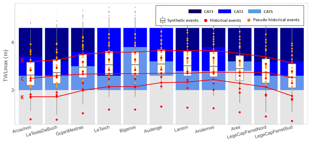
Figure 6 Categories of impact (CAT) related to TWL_max and repartition of the scenarios of the datasets: synthetic (box plots), historical (red points) and pseudo-historical (orange points). Red lines illustrate the variations of TWL_max for Klaus (K), Céline (C) and Xynthia (X).

Table 4 Number of events per category (CAT) in the learning database (Learn.), in the historical dataset (Histo.) and the pseudo-historical dataset (Pseudo.) used for validation.

This preliminary work highlighted the need to forecast water levels (TWL_max) and the associated categories of impact (CAT) for each municipality first, so that crisis managers can rely on predefined action plan typologies. Forecasting marine flood maps (H_max) should then be undertaken as a second step, in order to complement and refine the characterization of the event within each impact category. In the following, we thus propose different methods enabling to articulate the prediction of both TWL_max and H_max with different levels of accuracy.

3 (Meta)modeling methods and performance assessment

In this section, we describe the formal framework for setting up the ML-based models (named metamodels). Let us consider the maximum value of water height on land induced by flooding at the N spatial locations denoted ${\mathbf{H}}_{\text{max}}^i$ defined by their geographical coordinates $s=(s_{\mathrm{1}};s_{\mathrm{2}})$. We define ${\mathbf{H}}_{\text{max}}^i=\left({\mathbf{H}}_{\text{max}}^i\right({\mathit{s}}_{\mathrm{1}}),{\mathbf{H}}_{\text{max}}^i({\mathit{s}}_{\mathrm{2}}),\mathrm{\dots },{\mathbf{H}}_{\text{max}}^i({\mathit{s}}_N\left)\right)$ as the vector of H_max related to the ith model run defined by the vector of d offshore conditions ${\mathit{x}}^i=(x_{\mathrm{1}}^i,x_{\mathrm{2}}^i,\mathrm{\dots },x_d^i)$, and the n×N matrix ${\mathbf{H}}_{\text{max}}=[{\mathbf{H}}_{\text{max}}^{\mathrm{1}},{\mathbf{H}}_{\text{max}}^{\mathrm{2}},\mathrm{\dots },{\mathbf{H}}_{\text{max}}^n{]}^{\prime }$ built from the n numerical model's outputs. The objective is to predict H_max given x based on a statistical predictive model (named metamodel) that is trained with the learning dataset.

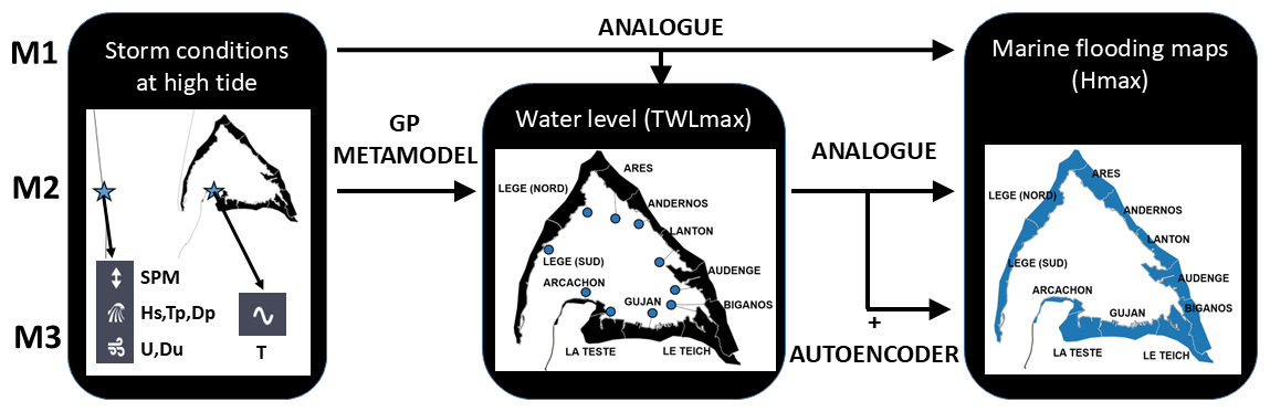
Figure 7 Diagram of the 3 methods named M1, M2 and M3 and main processes involved in the methods.

3.1 Description

3.1.1 M1: Analog-based approach

The first one, named “Analog”, is based on a look-up table approach. For given metocean forcing conditions, it consists in querying the learning database to identify the scenarios whose conditions that are the most similar, and retrieve the corresponding TWL_max and H_max maps. The result is named “analog” in reference to the approach commonly used in weather forecasting (e.g. Van den Dool, 2007). To measure the similarity, we use the distance named “EC” proposed by Camus et al. (2011) to both handle continuous and circular data (wind and wave direction). In this study, we only query one single analog, because our preliminary tests using multiple analogs (for instance the three analogs whose forcing conditions are the first three closest to the targeted one) have shown minor increase of the predictive capability of this approach.

3.1.2 M2: Combined Gp metamodel and analog

In this approach, we first predict the total water levels TWL_max from the metocean conditions at the reference points (outlined in white dots in Fig. 5) with a Gaussian process (denoted Gp) regression model (Williams and Rasmussen, 2006). On this basis, we identify, for each municipality, the analog flood map in the learning database whose TWL_max values are closest to those predicted by the GP-based model. The choice of the Gp model is guided by the high performance of this method as shown by multiple real case studies in coastal flooding (see e.g., Rohmer and Idier, 2012; Jia and Taflanidis, 2013; Perrin et al., 2020; Lopez-Lopera et al., 2020). In the following, we assume a Gp model with a linear trend, a Matérn 5$/$2 kernel model and a nugget effect. The hyper-parameters (parameters of the Gp model) are all evaluated through maximum likelihood estimation (e.g. Roustant et al., 2012). See further technical details in Appendix A.

3.1.3 M3: Combined Gp metamodel, analog and dimension reduction autoencoder

The third approach improves the second approach by predicting H_max from the forcing condition and TWL_max with a prediction based on the combined dimension reduction (denoted DR) – Gp metamodel approach that has been proposed in the literature (see for instance Jia and Taflanidis (2013) for hurricane-induced waves, Ma et al. (2022) for hurricane-induced surges, Li et al. (2020) in an estuary context, Perrin et al. (2020) for storm induced coastal flooding). To overcome the high dimensionality of the flood map (related to the number of pixels typically of several 10 000 s), the DR technique aims to extract a much smaller number (typically less than 10) of new variables (named latent) to represent the very high-dimensional output. Formally this consists in transforming H_max into a finite number of latent output variables

$$\begin{array}{rl}{\displaystyle }& {\displaystyle }\mathit{Z}=[{\mathit{z}}^{\mathrm{1}},{\mathit{z}}^{\mathrm{2}},\mathrm{\dots },{\mathit{z}}^n{]}^{\prime }\text{with}\\ {\displaystyle }& {\displaystyle }{\mathit{z}}^i=\left(z_{\mathrm{1}}^i,z_{\mathrm{2}}^i,\mathrm{\dots },z_{\mathrm{T}}^i\right)\text{so that}T\ll N.\end{array}$$

A popular approach is based on principal component analysis, denoted PCA (Jolliffe 2002). However, PCA is a linear technique, and it has been shown in our case to have limits (Rohmer et al., 2024a) due to the complexity of the flood maps, which have discontinuous heterogeneous patterns. Therefore, we preferably rely on a non-linear DR, namely a neural-network-based autoencoder, denoted AE (Baldi, 2012), in place of the popular PCA. For each of the latent variables, a Gp model is trained to link the latent variables to TWL_max forcing conditions. Recently Rohmer et al. (2021) have shown the added value of accounting for the dependence between the latent variables. To do so, we rely on the multi-output Gp model proposed by Gu and Berger (2016) (named the parallel partial kriging model). The AE architecture (number of nodes, number of layers, activation function) is selected so that the validation error is minimized as for Rohmer et al. (2024a) (see Appendix B for the comparison of architectures of autoencoders and Sect. 3.2 for the description of the validation procedure). Note that, if we recalculate H_max in the flooded area obtained with M2 with the combined dimension reduction (denoted DR) – Gp metamodel, we keep the flood extent from M2 to compensate the tendency of the chosen statistical approach to overestimate the flood extent (see Rohmer et al., 2024a). Thus, M3 can be considered a refinement of M2, as it uses the same methods to compute TWL_max and the flood extent, while improving the reconstruction of flood depth (H_max) through the use of an autoencoder.

3.2 Procedure for performance assessment

The objective is to measure to which extent the different approaches are respectively able to correctly predict TWL_max on the reference points and whole maps of H_max given “yet-unseen” offshore metocean conditions. Two approaches are used:

• The first approach relies on the available learning scenarios using a 10-fold cross-validation procedure (e.g., Hastie et al., 2009). This holds as follows: (1) the initial training dataset of input forcing conditions is randomly split into 10 equal sub-sets; (2) a sub-set is removed from the initial set, and a new Random Forest model is constructed using the remaining set; (3) the sub-set removed from the initial set constitutes the verification set and the differences between the true and the estimated value can then be estimated. In this procedure, the initial random split at step (1) may have some influence on the results. This can be minimized by repeating the procedure given number of times (typically 10 times).

• The second validation approach uses the set of independent samples that have not been used for the training. Here, we use the validation scenarios composed of historical and pseudo-historical events, represented with red and orange points on Fig. 6, that are in the range of the learning database (we exclude storm Domingos that occurred with a tidal coefficient below 40 but we keep all the Pseudo_Domingos_XX whose tidal coefficients are inside the tidal range of the learning database).

The prediction error is measured with the absolute error defined as at each location ${\mathit{s}}_{j=\mathrm{1},\mathrm{\dots },N}$:

$$\begin{array}{}\text{(1)}& {\text{AE}}^i\left({\mathit{s}}_j\right)=\left|{\mathbf{H}}_{\text{max}}^i\left({\mathit{s}}_j\right)-{\widehat{\mathbf{H}}}_{\text{max}}^i\left({\mathit{s}}_j\right)\right|,\end{array}$$

with ${\mathbf{H}}_{\text{max}}^i\left({\mathit{s}}_j\right)$ the true H_max at the jth location s ($j=\mathrm{1},\mathrm{\dots },N$) given the ith input offshore conditions ($i=\mathrm{1},\mathrm{\dots },n$), and ${\widehat{y}}^i\left({\mathit{s}}_j\right)$ is the reconstructed H_max map using the metamodel approach. A spatially averaged error indicator for the ith case is then defined as:

$$\begin{array}{}\text{(2)}& {\text{MAE}}^i=\mathrm{1}/N\sum _{j=\mathrm{1}}^N{\text{AE}}^i\left({\mathit{s}}_j\right),\end{array}$$

4 Results

4.1 Performance results from the cross-validation procedure

Figure 8 presents the results of the 10-fold cross validation on TWL_max and H_max for the three methods presented in Sect. 3. For TWL_max, the error corresponds to the difference between numerical simulations and metamodel-based predictions for each event on the reference points of each municipality (see Fig. 5). For H_max, the error corresponds to the Mean Absolute Error (or MAE, see Sect. 3.2 and Eq. 2) calculated for each municipality for the flooded nodes where H_max>0 in the numerical simulation (results of MAE for H_max=0 in the simulation are also provided in Appendix C to compare the performances of prediction of the flood extent).

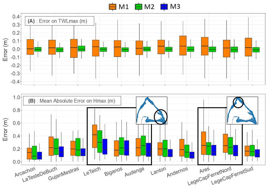
Figure 8 Error on TWL_max (A) and Mean Absolute Errors for H_max by restricting the analysis to the mesh nodes that are flooded, i.e. for H_max>0, in the numerical simulation (B) calculated with the 10-fold cross validation (Sect. 3.2). Box plots represent the 25th and 75th percentiles.

Concerning TWL_max, the analog-based approach (M1) enables to estimate the simulation results with a MAE of 10 cm in average, but for some cases it can reach up to 30 cm. On the other hand, using metamodels (in M2 and thus M3) enables to get closer to the target value within 5 cm most of the time and within 10 cm in all cases. On average, the uncertainty of M2/M3 predictions provided by the Gp model (via the kriging variance see Appendix A) is less than 4 cm which remains far below the ranges between categories of flooding presented in Sect. 2.4 (around 30 cm). When looking at H_max, we notice that the MAE decreases by introducing successively metamodel-based approaches to estimate TWL_max and H_max (from M1 to M3). With M3, the median of the MAE is below 20 cm whereas its ranges between 15 and 40 cm depending on the municipality for M1 and M2.

This first performance analysis based on cross validation shows that the two metamodels are correctly trained and improve the accuracy of TWL_max and H_max predictions. However, we can observe differences between the municipalities, with potentially higher MAE (up to 60 cm) on whose comprising wetlands (Le Teich, Biganos, Audenge, Ares). A first explanation is the deeper H_max expected on wetlands. To better understand the sources of errors, a deeper analysis is carried out in the next section with the validation dataset.

4.2 Predictive performance on pseudo-historical cases

The analysis of the predictive performance with validation cases presented on Fig. 9 reveals the same ranges of errors than the cross validation with a global improvement of the prediction of TWL_max and H_max from M1 to M3. However, some differences appear as predictions of TWL_max tend to be slightly overestimated for all the municipalities and M3 seems to perform better than in cross validation for municipalities with wetlands. These differences, due to the limited validation sample available, do not change the conclusions of Sect. 4.1.

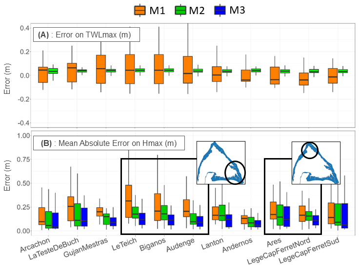
Figure 9 Errors on TWL_max (A) and Mean Absolute Errors on H_max by restricting the analysis to the mesh nodes that are flooded, i.e. for H_max>0, in the numerical simulation (B) calculated with the validation cases (Sect. 3.2). Box plots represent the 25th and 75th percentiles.

If the MAE on H_max enables to compare the prediction accuracy between the methods, it also aggregates different sources of errors depending on (1) the accuracy of TWL_max prediction (2) the marine flooding category (3) the exposure of the municipalities. To deepen this analysis, Fig. 10 provides the correlation between errors on TWL_max and H_max for each method (one point corresponds to the MAE of one municipality for one event). These plots show that:

• Higher errors on TWL_max logically lead to higher errors on H_max but some scenarios among the most important errors on H_max also present small errors on TWL_max.

• The maximum MAE on H_max do not always correspond to major flooding events (of CAT 2 or 3 outlined in light blue and cyan).

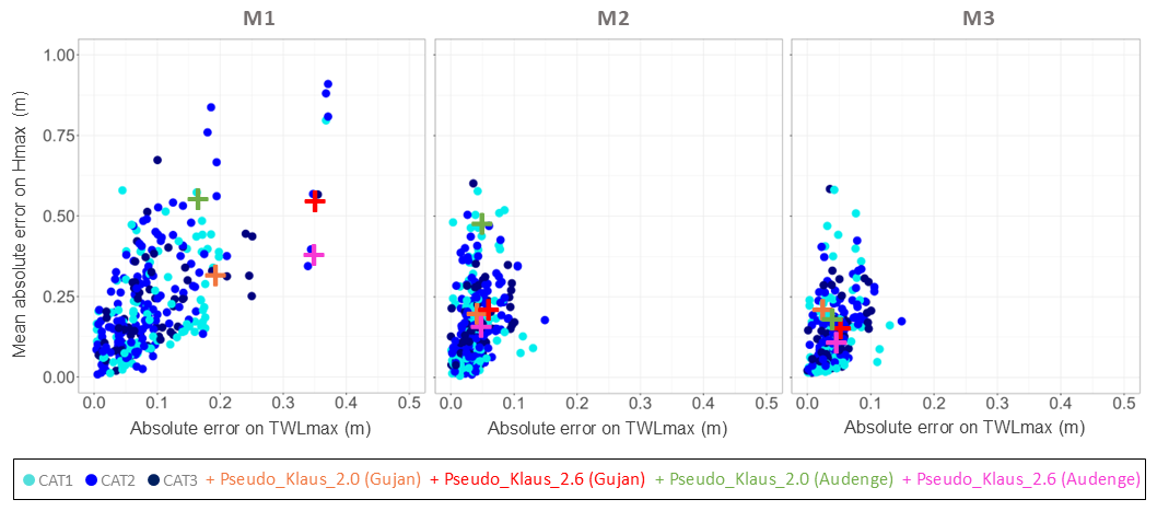
Figure 10 Relation between TWL_max and H_max errors for each method M1–M3. Each point represents the MAE calculated for one municipality and for one pseudo-historical event.

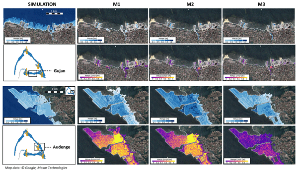
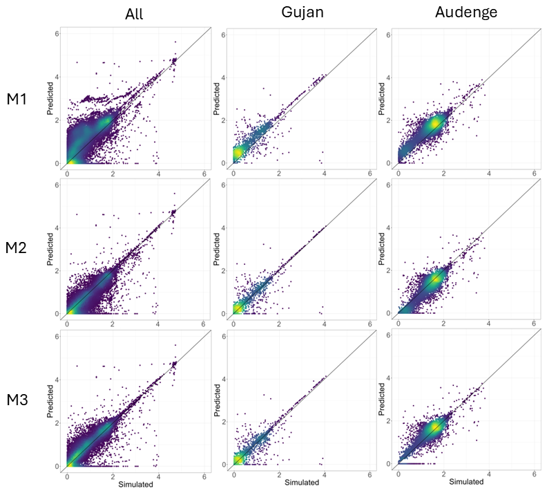
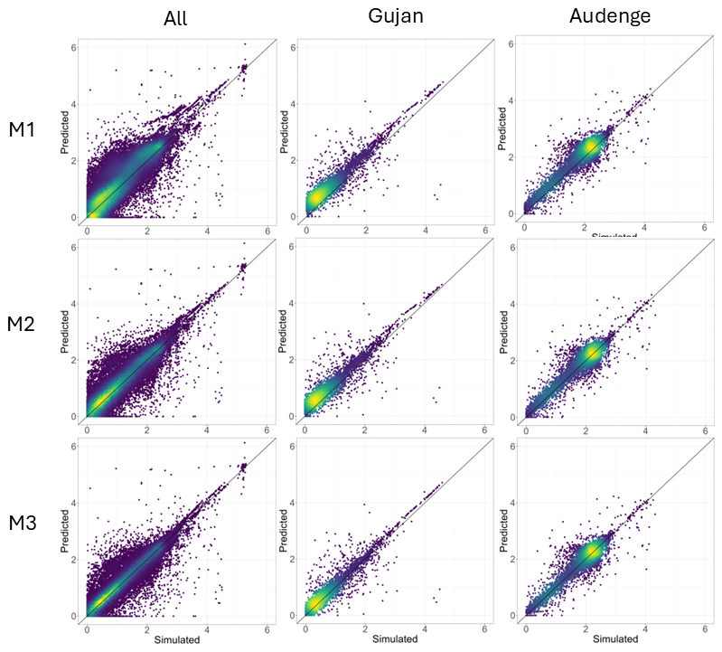
To investigate further, we focus the analysis on two examples that illustrate different situations in Gujan Mestras and Audenge, namely Pseudo_Klaus_2.0, that is characterised by a low-level category CAT 1, and Pseudo_Klaus_2.6, that is characterised by a high-level category CAT2-3. For these events, MAE on H_max for M2 and M3 remain quite high (between 20 and 50 cm) although TWL_max errors do not exceed 5 cm. The flooding and error maps plotted in Fig. 11 (for Pseudo_Klaus_2.0) and Fig. 12 (for Pseudo_Klaus_2.6) illustrate that, whatever the category of events, the maximum H_max errors are localized in the seafront quarters (like in Gujan-Mestras) or inside wetlands (like in Audenge). These sectors both present (1) a higher sensitivity to threshold effects on TWL_max which has a direct effect on seafront flooding and controls the quantity of water discharged into low lying areas and (2) greater water heights on land and then potential H_max prediction errors. Figures 10–12 also illustrate the improvement of marine flooding maps prediction from M1 to M3 both in terms of flooding extent and water height on land. Even for these cases with MAE of H_max above the median, the flooding maps reproduced with M2 and more particularly M3 are similar to the flooding maps obtained with the simulation of the numerical model. The scatter plots available in Appendix D (Figs. D1 and D2) confirm these results notably at the scale of the Arcachon lagoon with a significant improvement from M1 to M2 and similar patterns centred on the diagonal between M2 and M3.

Figure 11 H_max and H_max Absolute Errors (AE) for Pseudo_Klaus_2.0 at Gujan-Mestras (top) and Audenge (bottom) for the three methods. Map data: © Google, Maxar Technologies.

Figure 12 H_max and H_max Absolute Errors (AE) for Pseudo_Klaus_2.6 on Gujan-Mestras (top) and Audenge (bottom) for the three methods. Map data: © Google, Maxar Technologies.

To complete the comparison of the performance between the three methods, we analyse the confusion matrix on TWL_max and H_max (Fig. 13) to check how often (all municipalities, mesh nodes and validation scenarios combined) the right category of impact (through TWL_max) and the right H_max range (with classes of 50 cm commonly used for flood mapping) are predicted. This shows that the categories of impact (CAT) are quite well predicted by M1 (more than 70 % of the test cases) but globally better predicted by M2 and M3 (more than 90 % of the tests cases). This result agrees with the errors on TWL_max presented in Fig. 9 (potentially up to 20–30 cm for M1 and 10 cm for M2 and M3). The representation of the flood extent improves from M1 to M3 as evidenced by F1 score (that can be interpreted as a harmonic mean of the precision and recall, reaching its best value at 1 and worst value at 0) which reaches 0.94 for M1, 0.96 for M2 and 0.97 for M3. More precisely, the confusion matrix shows thatM1 allows to predict the correct order of magnitude only half of the time while M2 and M3 perform better with satisfactory predictions respectively around 65 % and 75 % of the time. More generally, M2 and M3 has a tendency of overestimation, but it should be underlined that the incorrect class is almost always the closest, i.e. when misclassifying the “0.5–1” class, the predicted one is often the “1–1.5”. From a risk perspective, this means that the approach minimises the false positives but tend to over-predict with more false positives.

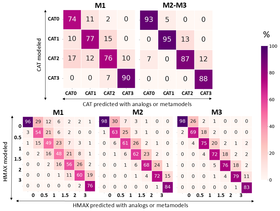
Figure 13 Confusion matrix (or error matrix) for the impact categories denoted CAT (computed based on TWL_max) (top) and H_max (bottom).

5 Discussion

Section 4 shows that the three methods can all be useful to predict maximum total water levels (TWL_max) as well as marine flooding category (CAT) and water height maps on land (H_max), each of them bringing some advantages (see Table 5):

• The analog-based approach (M1), although very simple, can provide interesting first order estimates of TWL_max, CAT and H_max but it can be limited and source of significant errors if the number of scenarios constituting the initial dataset is not enough to find sufficiently close analogs. Besides, the use of 6 input parameters to describe the storm conditions (U, Du, Hs, Tp, Dp, SPM) makes it difficult to evaluate if the selected analog overestimates or underestimates the target scenario, which can be delicate for operational forecast purposes.

• The approach combining Gp metamodels, analog and dimension reduction autoencoder methods (M3) is the most appropriate to jointly estimate with the highest accuracy, TWL_max (with a precision of 5 cm), CAT (90 % of the cases) and H_max (with a precision of 10 cm). It although requires more substantial implementation efforts, higher level of expertise, and uses statistical and machine learning methods that are still in the field of research for such forecasting purposes.

• Finally, the combined Gp metamodel and analog based approach (M2) turns out to be a good compromise between complexity/effort of implementation and accuracy. Through a quite simple statistical approach, it enables to estimate TWL_max and CAT with a good accuracy, which is an important first level of information for the crisis managers. Flooding maps are also quite well estimated, although less accurate than for M3 (with a higher prediction error for H_max on the order of 20 cm).

To sum-up, the analog-based approach can be seen as a valuable first step to explore the dataset and improve the understanding of flooding phenomena. On the other hand, for an operational forecasting context, the two metamodel-based approaches are more suitable for fast prediction and can be complementary depending on the type of event and the forecast lead time. While M2 may reach sufficient level of accuracy to give first order estimates of categories of impact and marine flooding maps at 72 or 48 h lead time (when uncertainties are still important), M3 may be more recommended at 24 or 12 h lead time when a detailed vision of the flood map is necessary. As pointed out by the national flood hazard recommendations (MEDDE, 2014) and the municipalities involved in the study, the first 10 cm class of H_max, is important for emergency services and crisis management as it determines the possibility to circulate easily for pedestrians and vehicles. Thus, M3 (with a precision of about 10 cm for H_max) is more suitable to predict H_max in areas with low H_max and also minimizes the errors on H_max classes of 50 cm range.

Table 5 Summary of prediction precisions and recommendations of use for the three methods. For TWL_max and H_max (h>0) the precision is an order of magnitude of the mean MAE for all municipalities, and all verification sets of cross validation. For CAT it corresponds to the percentage of correct predictions (all categories mixed up). For the flood extent it is a qualitative appreciation of the quality of the prediction based on Fig. 2B describing the errors for H_max (h=0).

Analysing the impact of uncertainties and the complementarity of different approaches for operational forecast is worth being further analysed with concrete cases of storm forecasting. This work, initiated in Rohmer et al. (2024b) will be continued and focused on applying these metamodel-based approaches (M2 and M3) with forecasts from Météo-France deterministic and EPS chains on recent events similarly as Dietrich et al. (2013) or Beuzen et al. (2019). These experiments will enable to carry out a complete analysis of the relative sources of uncertainties and to assess to which extent the metamodel error affects the spread of the probabilistic forecast, and whether it can be neglected compared to the variability in the metocean conditions (Rohmer et al., 2026).

Several lines for further improvements of the metamodeling methods are also identified. First, we focused in this study on the cases that led to flooding for the construction of the metamodels. Integrating also the case without flooding deserves to be investigated by testing different approaches either by completing the approach with a classification step (see e.g. Rohmer et al. (2018) for an example using a random forest classification technique) or using variants of Gaussian process metamodels adapted to zero-censored data (Spiller et al., 2023). More generally, this problem is related to the tendency of the metamodels to over-estimate the flood spatial extent, and more advanced approaches should be tested to improve this aspect by relying on more sophisticated deep learning techniques for instance based on generative models (e.g. Ma et al., 2024) combined with appropriate optimisation approaches to select the most optimal values of the ML model's parameters (called hyperparameters, see Bischl et al., 2023).

Finally, the global approach based on pre-calculated database is replicable on any type of marine flooding-prone area, and whatever the physical processes at stake, as it manages computation time issues by replacing real time numerical modelling by fast statistical tools. However, the methodological approaches and the associated conclusions regarding solution accuracy may vary depending on the environmental context, notably in wave overtopping prone areas and estuarine environments that are not considered in this study. In any case, the availability of the pre-calculated dataset enables to carry out an interesting preparatory work with potential users from municipalities or state services in preparedness phase to better assess the accurate thresholds, and the type and resolution of information required. This preparatory work is essential to allow the users to determine the criteria that will guide the whole developments and define the right level of complexity required to address operational needs.

6 Conclusion

In this study, we developed and compared three methods to predict marine flooding maps from offshore metocean conditions using successively analog-based approaches, regression type metamodels and deep learning techniques. The comparison, based on both technical accuracy and suitability for operational needs criteria, showed that the three methods all bring some advantages and drawbacks. If the efforts required to develop full metamodel approaches (including deep learning techniques) may be relevant for very urbanized sectors with civil security issues as the pilot site of Arcachon lagoon, the combination of more simple regression type models combined with analogs may be sufficient for applications at large scale or for natural or agricultural areas (where lower precision may be acceptable).

In this way, this work offers encouraging perspectives on the use of pre-calculated databases to carry out operational forecasts of marine flooding maps at local scale for different types of sites and geographical coverage. In particular, the capacity to predict quickly marine flooding maps opens up the possibility to address the issue of uncertainties though the production of ensemble forecasts and in-depth sensitivity analyses.

Appendix A: Kriging metamodeling

For a given $t=\mathrm{1},\mathrm{\dots },T$, each n-dimensional vector $z_t=(z_t^{\mathrm{1}},z_t^{\mathrm{2}},\mathrm{\dots },z_t^n)$ is assumed, in the context of kriging modelling (denoted KM), to be a realisation of a Gaussian process (Z_t(x)) with:

• mean (also named trend) ${\mathit{\mu }}_t\left(\mathit{x}\right)={\sum }_{j=\mathrm{1}}^d{b}_j{g}_j\left(\mathit{x}\right)$ (where g_j are fixed basis functions, and b_j are the regression coefficients of the d input variables);

• stationary covariance function $k_t(.,.)$ (named kernel) written as $\forall \mathit{x},{\mathit{x}}^{\prime }{k}_t(\mathit{x},{\mathit{x}}^{\prime })=\text{cov}\left(Z_t\right(\mathit{x}),Z_t({\mathit{x}}^{\prime }\left)\right)$.

For new offshore forcing conditions x^∗, the predictive probability distribution $Z_t\left({\mathit{x}}^{\ast }\right)\mathrm{|}\mathit{\left\{}{Z}_t\right({\mathit{x}}^{\mathrm{1}})=z_t^{\mathrm{1}},\mathrm{\dots },Z_t({\mathit{x}}^n)=z_t^n$ follows a GP with mean ${\widehat{z}}_t\left({\mathit{x}}^{\ast }\right)$ and variance $s_t^{\mathrm{2}}\left({\mathit{x}}^{\ast }\right)$ defined using the universal kriging equations (e.g. Roustant et al., 2012) as follows:

$$\begin{array}{}\text{(A1)}& {\displaystyle }& {\displaystyle }{\widehat{z}}_t\left({\mathit{x}}^{\ast }\right)=\mathit{g}({\mathit{x}}^{\ast }{)}^{\prime }\widehat{b}+\mathit{c}({\mathit{x}}^{\ast }{)}^{\prime }.{\mathit{C}}^{-\mathrm{1}}.({\mathit{z}}_t-\mathit{G}\widehat{b}),\text{(A2)}& {\displaystyle }& {\displaystyle }\begin{array}{rl}{\displaystyle }{s}_t^{\mathrm{2}}\left({\mathit{x}}^{\ast }\right)=& {\displaystyle }{V}_S+\left(\mathit{g}\right({\mathit{x}}^{\ast }{)}^{\prime }\widehat{b}-\mathit{c}({\mathit{x}}^{\ast }{)}^{\prime }.{\mathit{C}}^{-\mathrm{1}}.\mathit{G}{)}^{\prime }\\ {\displaystyle }& {\displaystyle }.({\mathit{G}}^{\prime }.{\mathit{C}}^{-\mathrm{1}}.\mathit{G}{)}^{-\mathrm{1}}.(\mathit{g}({\mathit{x}}^{\ast }{)}^{\prime }\widehat{b}-\mathit{c}({\mathit{x}}^{\ast }{)}^{\prime }.{\mathit{C}}^{-\mathrm{1}}.\mathit{G}),\end{array}\end{array}$$

where ${\mathit{z}}_t=\left(Z_t\right({\mathit{x}}^{\mathrm{1}})=z_t^{\mathrm{1}},\mathrm{\dots },Z_t({\mathit{x}}^n)=z_t^n)$, C is the n×n covariance matrix between the points $Z_t\left({\mathit{x}}^{\mathrm{1}}\right),\mathrm{\dots },Z_t\left({\mathit{x}}^n\right)$ whose element is $C[i,j]=k_t\left({\mathit{x}}^i{\mathit{x}}^j\right)$; c(x^∗) is the n-dimensional vector composed of the covariance between Z_t(x^∗) and the points $Z_t\left({\mathit{x}}^{\mathrm{1}}\right),\mathrm{\dots },Z_t\left({\mathit{x}}^n\right)$; g(x^∗) is the d-dimensional vector of trend functions values at x^∗, $\mathit{G}=\left(\mathit{g}\right({\mathit{x}}^{\mathrm{1}}),\mathrm{\dots },\mathit{g}({\mathit{x}}^n){)}^{\prime }$ is the n×d experimental matrix, the best linear estimator $\widehat{\mathit{b}}$ of b is $({\mathit{G}}^{\prime }{\mathit{C}}^{-\mathrm{1}}\mathit{G}{)}^{-\mathrm{1}}{\mathit{G}}^{\prime }{\mathit{C}}^{-\mathrm{1}}{\mathit{m}}_Y$, and $V_S={\mathit{\sigma }}^{\mathrm{2}}-\mathit{c}({\mathit{x}}^{\ast }{)}^{\prime }.{\mathit{C}}^{-\mathrm{1}}.\mathit{c}({\mathit{x}}^{\ast })$ by assuming $k(.,.)$ to be stationary with σ² a hyperparameter (named process variance) to be estimated.

Appendix B: Autoencoder

This method belongs to the class of deep neural networks whose typical architecture is depicted in Fig. B1. It consists of an input layer (left blue layer in Fig. B1), a given number of hidden layers (light-coloured layers), and an output layer (right green layer). The process of going from the input layer to the hidden layer is called encoding, (i.e. from the original data y to latent variables z), while the process of going from the hidden layer to the output layer is called decoding (i.e. from latent variables z to the variables back-transformed in the physical domain $\widehat{y}$). The central layer is named the bottleneck hidden layer and provides the latent variables z. The AE architecture can be parametrised in different manners (Pawar and Attar 2019), i.e. the number of nodes of the hidden layer, the number of nodes of the and bottleneck layer (i.e. the number of latent variables), the type of activation function applied to each node, etc.

To select the parameters of the AE architecture, we conducted the 10-fold cross validation procedure by assuming different assumptions, namely by varying the number of nodes of the hidden layer from 10–50, the number of latent variables from 3–5, the type of activation function among relu and sigmoid for the hidden layer and among linear, tanh and selu. Figure B2 shows the cross-validation prediction error, here measured by the root mean square error denoted RMSE, for two sectors, Gujan-Mestras and Andernos. This indicates that having 10 nodes in the hidden layer with relu activation, and 3 in the bottleneck with tanh allows to achieve the lowest prediction error for mesh nodes with H_max>0 and H_max=0 in the numerical simulation. This result was also confirmed for the other sectors on the Arcachon lagoon.

Figure B1 Typical autoencoder architecture.

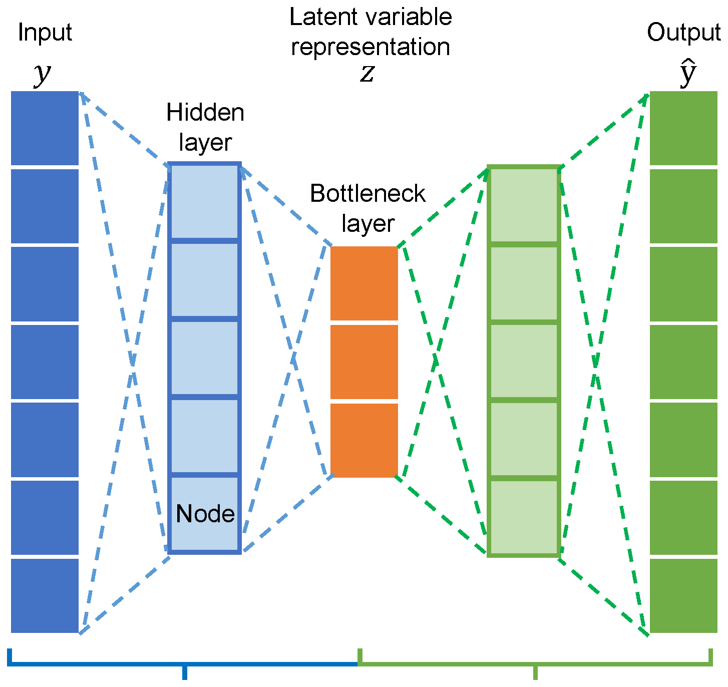
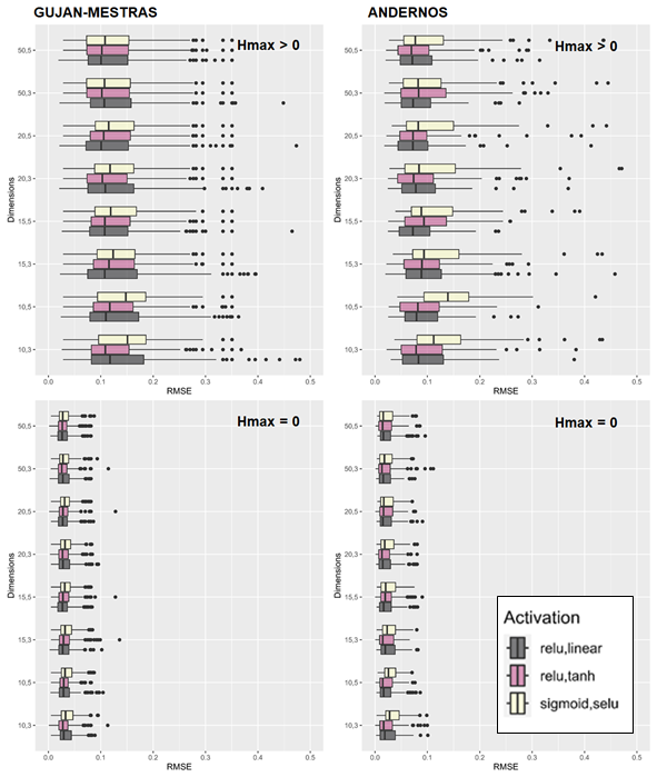
Figure B2 Evolution of the cross-validation prediction error, here measured by the root mean square error denoted RMSE, for two sectors, Gujan-Mestras (left) and Andernos (right) for mesh nodes with H_max>0 (top) and H_max=0 (bottom) in the numerical simulation.

Appendix C: MAE for H_max=0 in the simulation for the cross validation

The cross-validation-based MAE calculated for non-flooded mesh nodes, i.e. with H_max=0 in the numerical simulation, shows a clear decrease from M1 to M3. This indicates that M3 achieves the most accurate prediction of the flood spatial extent, i.e. here corresponding to the total number of mesh nodes predicted with H_max=0 while being non-flooded in the numerical simulation. This suggests also that M3 enables to decrease the rate of false alarms, though we notice that MAE remains non-zero (of the order of less than 1 cm), hence reflecting a remaining tendency of M3 to slightly over-estimate the flood extent.

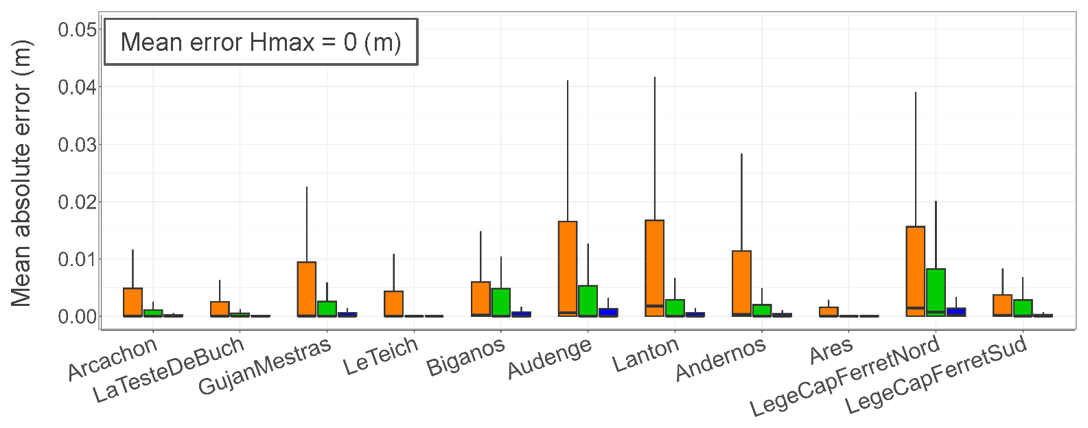
Figure C1 Mean absolute error (MAE) calculated over the non-flooded mesh nodes (with H_max=0 in the numerical simulations) of each municipality from the cross-validation procedure.

Appendix D: Scatter plots

Figure D1 Scatter plot of predicted vs. simulated H_max for Klaus_2.0.

Figure D2 Scatter plot of predicted vs. simulated H_max for Klaus_2.0.