Revealing the structure of heavy precipitation events: a spatio-temporal wavelet approach

The impact of a heavy precipitation event is determined not only by the total amount of precipitation, but also by its spatial and temporal distribution. This study introduces a framework to quantify key spatiotemporal properties of precipitation events – namely their characteristic time, length and speed – based on radar observations. The method employs a wavelet-based spectral filtering approach to isolate precipitation signals at distinct temporal and spatial scales.

Focusing on Germany, we analyse 100 heavy precipitation events from the high-resolution RadKlim dataset. We assess the physical consistency of the derived characteristics and examine their links to large-scale atmospheric dynamics. Our results reveal systematic patterns in the spatiotemporal structure of heavy precipitation events. The proposed framework provides a robust basis for process-oriented analysis and offers potential for improved risk assessment and climate studies.

1 Introduction

Heavy precipitation events repeatedly attract attention due to their catastrophic socioeconomic impacts. Recent examples in Europe include the flooding events of July 2021 and May/June 2024 in Germany, as well as the severe flood episode in Emilia-Romagna, Italy, in May 2023 (Friederichs et al., 2024; Tradowsky et al., 2023; Arrighi and Domeneghetti, 2024). Taken together, these events demonstrate that extreme precipitation events pose a growing challenge for communities and policymakers and underscore the urgent need to better understand the underlying physical processes and possible changes in their characteristics in the context of ongoing climate change.

Precipitation manifests across a broad spectrum of spatial and temporal scales, ranging from short-lived, localized convective events to long-lasting, synoptic-scale stratiform systems. The diverse physical processes governing these systems complicate efforts to robustly quantify changes in their frequency and intensity, as the inherent internal variability can mask underlying climate signals (Fischer and Knutti, 2016). A major focus of recent research has thus been the development of approaches that better capture precipitation processes at finer scales, in order to investigate the processes through which climate change affects heavy precipitation events. These efforts include convection-permitting model simulations (Hundhausen et al., 2025) and storyline approaches (Shepherd et al., 2018), but also stochastic modelling frameworks have gained increasing attention as means to generate physically plausible small-scale precipitation structures (Northrop, 2024). Beyond the development of high-resolution datasets, there is a need for novel stochastic methods for evaluating and analysing scale-dependent signals in precipitation data.

In dynamical meteorology, scale analysis is applied to determine the dynamic regimes of a system. It uses three fundamental metrics – characteristic length L, characteristic time T and characteristic speed V – to assess fundamental balances (see Kraus, 2004; Thunis and Bornstein, 1996). Such traditional approaches characterize the dynamical system at prescribed spatial and temporal scales. In this context, precipitation events are investigated based on various duration thresholds to examine different temporal scales. One example are intensity-duration-frequency curves to describe the temporal scaling of precipitation (Koutsoyiannis et al., 1998). The spatial extent of precipitation events is then assessed by counting the number of grid boxes affected by precipitation (Hundhausen et al., 2024; Voit and Heistermann, 2022; Lochbihler et al., 2017). The CatRaRe catalogue (Lengfeld et al., 2025), provided by the German Meteorological Service (DWD), uses the duration and affected area of the respective event to characterise precipitation events by their space-time characteristics. Although such duration-based methods are intuitive and widely used, they suffer from an inherent redundancy: precipitation accumulations over longer periods inevitably include contributions from shorter accumulation periods. As a result, different duration classes do not provide independent representations of distinct precipitation-generating processes, but rather constitute nested aggregations of the same underlying signal.

The key idea in this paper is that knowledge of typical scales in the precipitation field allows us to draw conclusions about the processes that generate the precipitation field – in the spirit of a scale analysis that tells us which characteristic dynamics prevail at specific scales. We present a method for the quantitative assessment of the spectral properties of an event simultaneously in space and time. Our analysis concentrates on heavy precipitation events, and we demonstrate how these characteristic quantities can be estimated using wavelet-based methods. The approach provides insight into the underlying processes, as spatial and temporal scales are characteristic of specific precipitation regimes. For example, an increased contribution of convective precipitation is expected to result in enhanced small-scale variability. This is reflected in the seasonal cycle: over Germany, the average spatial scale of precipitation events in summer is significantly smaller than in winter, consistent with the increased frequency of convective precipitation events (Lengfeld et al., 2020). Spectral filtering can separate temporal and spatial scales in an orthogonal and non-overlapping manner, allowing process-relevant variability to be isolated without redundancy. This approach not only facilitates the identification of distinct physical processes, but also enhances the detection of climate signals that may be obscured in the raw data.

In this paper, we propose a spectral decomposition method for quantitatively analysing the spatiotemporal properties of precipitation events. Our method is based on the wavelet transform (WT), a technique that has been widely adopted across scientific disciplines for filtering signals at different scales. WT is used because its decomposition is based on localised basis functions. Unlike sinusoidal Fourier basis functions, for example, wavelets are particularly well suited to capturing both short-lived and long-lived non-periodic features in a signal (Mallat, 1989; Daubechies, 1992). Moreover, the WT has been used extensively in the analysis of spatial precipitation data, thereby demonstrating its usefulness in various contexts, including the verification of spatial precipitation fields (Casati et al., 2004; Yano and Jakubiak, 2016; Buschow and Friederichs, 2021), quantification of convective organization (Brune et al., 2021), and the analysis of climate change signals (Buschow, 2023; Benestad et al., 2022).

Wavelets in one, two and three dimensions, as well as corresponding algorithms, are available (Selesnick and Li, 2003; Kingsbury, 1998). A common limitation is that wavelet filtering typically requires uniform grids in all dimensions. A two-dimensional decomposition along the horizontal axes with a uniform scale is dynamically consistent, as the two horizontal directions differ very little dynamically. In a three-dimensional context, however, this becomes difficult because the vertical direction behaves very differently in terms of spatial scale and is often measured not in meters, but in hectopascals, for example. Here, both directions can be linked via an energy metric. If the third dimension is time, the intuitive connection between the scales of the dimensions is missing. For propagating Gaussian random fields, it is the speed that links space and time. Precipitation, however, exhibits multiscale behaviour (Foufoula-Georgiou and Krajewski, 1995), which can involve different propagation speeds at different spatial scales. Using three-dimensional wavelet analysis, it is possible to investigate such multiscale behaviour (Yano, 2010). We combine a one-dimensional WT in time with a two-dimensional WT in space, following an approach carried out by Yano and Jakubiak (2016) in two dimensions, to achieve a joint analysis of the spatial and temporal scales underlying precipitation events. In principle, the proposed method can be applied to any data set that is defined on a uniform spatiotemporal grid and does not contain any missing values. In practice, computational capacities limit the manageable data size. This study aims to provide new scale-aware analysis approaches for assessing changes in heavy precipitation events, taking into account that changes can manifest themselves differently at different scales.

The focus of this study is on precipitation over Germany, motivated by the availability of high-resolution, radar-based precipitation data. In particular, we use the RadKlim dataset provided by DWD, which offers a continuous time series of hourly precipitation data from 2001 to 2024 (Lengfeld et al., 2020). Our analysis concentrates on the 100 most extreme precipitation events that occurred during the summer months over Germany, in order to investigate their spatiotemporal characteristics. Using a WT, we quantify the dominant spatial and temporal scales of each event. From these, we derive the characteristic length and time, and two independent descriptors–the characteristic scale and the characteristic speed–which provide a compact, physically meaningful representation of precipitation events. We demonstrate that these parameters are closely related to atmospheric dynamics, thereby confirming the physical plausibility of our approach. By linking event-scale properties to larger-scale processes, this study deepens our understanding of how precipitation extremes organize in space and time. The proposed metrics have a wide range of uses beyond the scope of this study. These include quality assessment and intercomparison of datasets, as well as evaluation of climate projections (e.g. CMIP).

This paper is organized as follows. In Sect. 2, we present the theoretical background for the proposed space–time decomposition approach. Section 3 describes the data and preprocessing steps in detail. In Sect. 4.1, we analyse selected representative cases, followed by a comprehensive evaluation of the top 100 events in Sect. 4.2. The connection to the underlying dynamics and thermodynamics is investigated in Sect. 5. Finally, Sect. 6 summarizes the main findings and provides a discussion of their implications.

2 Theory

A variety of wavelet types – or wavelet families, exist, ranging in complexity from simple step-function wavelets (Haar, 1909) to more advanced formulations. Each wavelet family is characterized by specific properties such as smoothness, symmetry, and vanishing moments, which make it more or less suitable for capturing different features in a signal. For a comprehensive introduction to wavelet theory, the interested reader is referred to standard references such as Daubechies (1992) and Mallat (1998).

In this study, we employ the complex Dual-Tree wavelet which has proven effective for the analysis of spatial precipitation fields (Buschow and Friederichs, 2021; Brune et al., 2021). The Dual-Tree Complex WT (DT-ℂWT) and the algorithm for its computation, were introduced by Kingsbury (1998). Compared to more traditional, real value wavelet families, such as Haar or Daubechies wavelets, the ℂWT exhibits improved shift invariance, meaning that its coefficients are more robust to small spatial and temporal displacements of the signal (Kingsbury, 1998). In principle, the proposed method can be implemented with any wavelet family. We tested several alternatives, including Haar and Daubechies wavelets, but did not observe any substantial performance advantage over the ℂWT in terms of computational efficiency. The DT-ℂWT, like other WTs, satisfies Parseval's energy theorem, an energy conservation principle stating that the L²-norm of the original signal equals the L²-norm of its wavelet coefficients (Kingsbury, 1998). This ensures that the transform preserves the total energy of the precipitation field across scales.

2.1 Discrete wavelet transform in one & two dimensions

We begin by introducing the one-dimensional discrete wavelet transform and will refer to its parameters using the subscript _T throughout this text, since it is applied to the time component here. Let h(t) be a signal defined over discrete time steps t₁, …, $t_{n_T}$ where n_T is a power of two. Let ψ(t) denote a wavelet function, with daughter wavelets ${\mathit{\psi }}^{k_T,j_T}\left(t\right)$ defined as

$$\begin{array}{}\text{(1)}& {\mathit{\psi }}^{k_T,j_T}\left(t\right)={\displaystyle \frac{\mathrm{1}}{\sqrt{{\mathrm{2}}^{j_T}}}}\mathit{\psi }\left({\displaystyle \frac{t-k_T{\mathrm{2}}^{j_T}}{{\mathrm{2}}^{j_T}}}\right).\end{array}$$

j_T and k_T are discrete parameters controlling the scale and translation of the wavelet along the time axis, thereby enabling the analysis of spectral energy at different temporal scales and positions. The wavelet coefficients d(k_T,j_T) represent the amplitude of the signal h(t) at a given scale j_T and temporal position k_T and are defined as

$$\begin{array}{}\text{(2)}& d^{j_T}\left(k_T\right)={〈h\left(t\right),{\mathit{\psi }}^{k_T,j_T}\left(t\right)〉}_t,\end{array}$$

with $\langle \cdot ,\cdot {\rangle }_t$ denoting the inner product in time.

To extend the wavelet analysis to two dimensions, we consider a signal g(x,y), where x in x₁, …, $x_{n_{XY}}$ and y in y₁, …, $y_{n_{XY}}$ denote discrete spatial coordinates. This kind of WT requires that x and y have the same length n_XY and, analogous to the one-dimensional case, that n_XY is a power of two. The respective parameters are denoted with the subscripts _X and _Y, for the individual parameters, or _XY for parameters that are equal in both dimensions.

The two-dimensional wavelets are scaled by a common scale parameter j_XY and translated along the x- and y-axes by k_X and k_Y, respectively, to cover different spatial positions. Directional information can be incorporated through an orientation parameter q (see, e.g., Daubechies, 1992). This leads to the following definition of the daughter wavelets of the two-dimensional wavelet function ψ(x,y)

$$\begin{array}{}\text{(3)}& \begin{array}{rl}& {\mathit{\psi }}_q^{(k_X,k_Y),j_{XY}}(x,y)=\\ & {\displaystyle \frac{\mathrm{1}}{{\mathrm{2}}^{j_{XY}}}}{\mathit{\psi }}_q\left({\displaystyle \frac{x-k_X{\mathrm{2}}^{j_{XY}}}{{\mathrm{2}}^{j_{XY}}}},{\displaystyle \frac{y-k_Y{\mathrm{2}}^{j_{XY}}}{{\mathrm{2}}^{j_{XY}}}}\right),\end{array}\end{array}$$

and the two-dimensional wavelet coefficients

$$\begin{array}{}\text{(4)}& d_q^{j_{XY}}(k_X,k_Y)={〈g(x,y),{\mathit{\psi }}_q^{(k_X,k_Y),j_{XY}}(x,y)〉}_{x,y},\end{array}$$

with $\langle \cdot ,\cdot {\rangle }_{x,y}$ denoting the inner product in space. The wavelet coefficients $d_q^{j_{XY}}(k_X,k_Y)$ characterize the localized spectral properties of g(x,y) across scales j_XY, locations (k_X,k_Y) and orientations q. According to the Parseval theorem, the spectral energy at each scale is given as the L²-norm of the wavelet coefficients, which for the one- and two-dimensional cases are

$$\begin{array}{}\text{(5)}& {\displaystyle }{e}^{j_T}=\sum _{k_T}{\left|d^{j_T}\left(k_T\right)\right|}^{\mathrm{2}},\text{(6)}& {\displaystyle }{e}^{j_{XY}}=\sum _q\sum _{(k_X,k_Y)}{\left|d_q^{j_{XY}}(k_X,k_Y)\right|}^{\mathrm{2}}.\end{array}$$

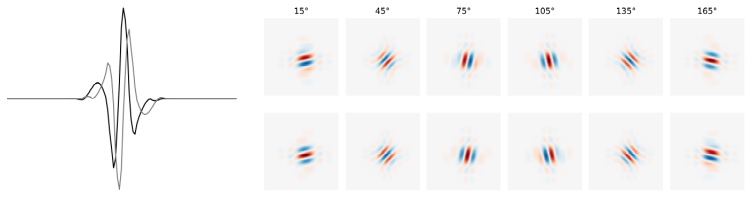
Figure 1 Illustration of the complex Dual-Tree wavelet in one (left) and two dimensions (right). In one dimension, the real and imaginary parts of the wavelet are shown by the black and gray lines, respectively. In two dimensions, the real and imaginary components are displayed in the top and bottom rows, with columns corresponding to different wavelet orientations (15, 45, 75, 105, 135 and 165°).

Figure 1 illustrates the complex Dual-Tree wavelet in one and two dimensions. An important feature is that the real and imaginary parts are phase-shifted relative to each other, forming an approximately analytic and rotation invariant wavelet (Selesnick, 2002).

2.2 Discrete wavelet transform in spatiotemporal space

For the three-dimensional WT, we consider a signal $f(x,y,t)$, encompassing spatial and temporal dimensions as pointed out in Sect. 2.1. A rather intuitive approach is to extend the DT-ℂWT to three dimensions (Selesnick and Li, 2003), in which case the complex wavelet coefficients is expressed as

$$\begin{array}{}\text{(7)}& \begin{array}{rl}& d_q^{j_{XYT}}(k_X,k_Y,k_T)=\\ & {〈f(x,y,t),{\mathit{\psi }}^{(k_X,k_Y,k_T),j_{XYT}}(x,y,t)〉}_{x,y,t}.\end{array}\end{array}$$

The scaling parameter j_XYT of the 3D wavelet determines the resolution of all three dimensions simultaneously. As a result, it is very difficult to determine the scale changes in space and time separately. This limitation is analogous to the two-dimensional transform, where a single scaling parameter j_XY controls both the x and y dimensions (see Sect. 2.1). To address this limitation, we adopt a hybrid approach that separates spatial and temporal scales. Specifically, we apply a one-dimensional WT along the temporal dimension t and a two-dimensional WT for the spatial fields on (x,y). The calculation of the wavelet coefficients is then as follows:

$$\begin{array}{}\text{(8)}& \begin{array}{rl}& d_q^{j_{XY},j_T}(k_X,k_Y,k_T)=\\ & {〈\langle f(x,y,t),{\mathit{\psi }}^{k_T,j_T}\left(t\right){\rangle }_t,{\mathit{\psi }}_q^{(k_X,k_Y),j_{XY}}(x,y)〉}_{x,y}.\end{array}\end{array}$$

By doing so, we decouple the spatial and temporal scales, and provide individual scaling parameters for the spatial and temporal scales. This allows for an interpretable analysis of spatiotemporal characteristics within the signal $f(x,y,t)$. Following Eqs. (5) and (6), we then summarize the spectral energies as combinations of spatial and temporal scales using

$$\begin{array}{}\text{(9)}& e^{j_{X,Y},j_T}=\sum _q\sum _{k_t}\sum _{k_x,k_y}{\left|d_q^{j_{X,Y},j_T}(k_X,k_Y,k_T)\right|}^{\mathrm{2}}.\end{array}$$

Our implementation is primarily based on the open-source Python package DTCWT (Wareham et al., 2017). It offers an implementations of the 1D, 2D and 3D DT-ℂWT based on the multiresolution approximation (MRA) algorithm (Mallat, 1989), which is typically applied for discrete wavelets. We first apply the 1D DT-ℂWT and obtain wavelet coefficients at each grid point. Subsequently, a 2D DT-ℂWT is applied at each scale. The resulting wavelet coefficients are then converted into spectral energies according to Eq. (9). The restrictions on n_T and n_XY to be powers of two, as mentioned above, are a direct consequence of the MRA algorithm. As a second consequence, we yield estimates of spectral energies only for the discrete spatial and temporal scales j_T=2⁰, 2¹, …, n_T and j_XY=2⁰, 2¹, …, n_XY.

To derive the characteristic length $L={\stackrel{\mathrm{‾}}{j}}_{XY}$ and characteristic time $T={\stackrel{\mathrm{‾}}{j}}_T$ from the spectral energies $e^{j_{XY},j_T}$ (Eq. 9), we essentially follow Buschow (2022) and compute the centre of mass as the average scales, weighted by the spectral energies:

$${\stackrel{\mathrm{‾}}{j}}_{XY}={\displaystyle \frac{{\sum }_{j_T}{\sum }_{j_{XY}}{j}_{XY}{e}^{j_{XY},j_T}}{{\sum }_{j_T,j_{XY}}{e}^{j_{XY},j_T}}}$$

and

$$\begin{array}{}\text{(10)}& {\stackrel{\mathrm{‾}}{j}}_T={\displaystyle \frac{{\sum }_{j_{XY}}{\sum }_{j_T}{j}_T{e}^{j_{XY},j_T}}{{\sum }_{j_T,j_{XY}}{e}^{j_{XY},j_T}}}.\end{array}$$

From these two characteristic properties, we derive the characteristic speed of the precipitation system as $V=L/T$. We further define a combined space-time scale, which we refer to as the characteristic scale S as:

$$\begin{array}{}\text{(11)}& S=\sqrt{{\left({\displaystyle \frac{L}{\mathrm{SD}\left(L\right)}}\right)}^{\mathrm{2}}+{\left({\displaystyle \frac{T}{\mathrm{SD}\left(T\right)}}\right)}^{\mathrm{2}}}.\end{array}$$

By scaling L and T by their respective standard deviations, which we calculate across all events considered in this study, we obtain dimensionless quantities that can be meaningfully combined despite originating from different units and value ranges. Analogously, the centre of mass can be derived from either the one- or two-dimensional WT, in which case we obtain an estimate at each timestep for the characteristic length L(t) or at each gridpoint for the characteristic time T(x,y).

The method presented here is applicable to any three-dimensional data set defined on a uniform grid without missing values. E.g. an application to data sets comprising three spatial dimensions, including the horizontal height is possible. However, When analysing further variables, such as temperature or wind speed alternative wavelet families may be more appropriate to ensure an optimal representation and filtering of the underlying signal characteristics. In the present study, we employ a combination of a 2D WT and 1D WT to distinguish between spatial and temporal scales. Alternatively, a combination of three 1D WTs would allow a full separation of the three dimensions considered here (i.e. the x-, y-directions and time).

3 Data & Preprocessing

This study utilizes hourly precipitation totals from RadKlim, version 2017.002, provided by DWD (Winterrath et al., 2018). RadKlim is a high-resolution climatological dataset, provided on a 1 km × 1 km grid which has been specifically developed to improve the understanding of precipitation dynamics and to support applications in climate research, hydrology, and risk assessment. The dataset combines radar-based precipitation estimates with observations from over 1000 ground-based gauges, using advanced correction algorithms to reduce radar-related biases. Temporal consistency is maintained through standardized processing and harmonized radar calibration. The record begins in 2001 and is updated annually, covering the period from 2001 to 2024 at the time of writing.

For our analysis in Sect. 5, we further apply data from the ERA5 reanalysis data (Hersbach et al., 2025). Specifically, we use daily mean wind speed at the pressure levels 300, 500, 700, 850, and 1000 hPa, and the convective time scale τ (Done et al., 2006). The selected pressure levels cover all relevant atmospheric layers, ranging from near-surface conditions (1000 hPa) through the lower and mid-troposphere (850–500 hPa) up to the upper troposphere (300 hPa), thereby providing a vertically comprehensive representation of the atmospheric state. The convective timescale τ is defined as the ratio between convective available potential energy (CAPE) and the rate at which CAPE is consumed by convection. It quantifies how rapidly potential energy is converted into convective motion. Small values of τ indicate stronger large-scale forcing, whereas large τ correspond to airmass convection with only weak forcing from larger scales. Both variables are averaged over the same spatiotemporal window which is used for the WT, i.e. a 4 d window over Germany (see Sect. 3.2). This large-scale averaging reduces the relevance of convection-permitting processes, which supports our choice of ERA5 data instead of smaller-scale, convection-permitting datasets. Further, at the time of writing, convection-permitting simulations with a spatial and temporal coverage consistent with the RadKlim dataset were not available.

3.1 Event identification

From the available time period, we aim to identify intense precipitation events during the northern hemispheric summer months (June to August) for further analysis. We consider an event to be intense if the total amount of precipitation within a limited area and a limited time is particularly high. Specifically, we select the top 100 events based on the total precipitation volume accumulated within a 2 d window over a spatial domain of 50 km × 50 km. An area measuring 50 km × 50 km is relatively small compared to the area affected by heavy precipitation events. It is primarily intended to cover the core area of maximum precipitation and is used exclusively for event detection in this study. The location and intensity of the recorded events are shown in Fig. 2, with known extreme precipitation events with severe impacts over Germany among the six strongest events. This choice of temporal and spatial thresholds is to some extent arbitrary. However, we consider it a reasonable approximation for capturing high-impact events. To avoid temporal clustering, events are required to be separated by at least 72 h. The choice of 72 h has no impact on the number of events and we consider this time interval to be long enough to ensure the independence, given that typical precipitation events in Germany tend not to exceed it.

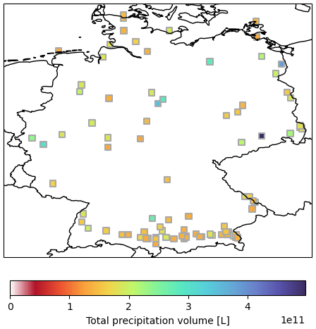
Figure 2 Center location and total precipitation amount [L] of the top 100 precipitation events in Germany, in terms of their 2 d × 50 km × 50 km total precipitation volume (colour) during the northern hemispheric summer months (June–August).

As a consistent, impact-oriented measure of event intensity throughout this paper, we use the total precipitation volume within this region and time period for each event. There are multiple approaches to defining extreme precipitation events. One alternative we considered was the use of predefined events, such as those listed in the DWD CatRaRe catalogue (Lengfeld et al., 2025). However, our results are not sensitive to the specific choice of event definition, as the main findings remain robust across different selection approaches.

3.2 Data preprocessing

To analyse the identified events, we use a much larger space-time window to ensure that we capture the entire spatial and temporal extent of each event. Specifically, we analyse each event over a 4 d window centred on the precipitation peak (±48 h) and across the entire spatial domain of RadKlim. This approach allows us to avoid manually defining the temporal or spatial boundaries of each event, which would require arbitrary thresholds or other subjective criteria. While this may include some precipitation not directly associated with the main event, its effect is considered negligible, as such additional rainfall is generally weak and does not significantly alter the overall signal.

Extreme precipitation events are rarely confined to national or regional boundaries. Consequently, the RadKlim dataset may not fully capture their complete spatial extent, a limitation commonly recognized in the analysis of large-scale hydro-meteorological extremes. For instance, the 2021 Ahr flooding required combining Belgian and German precipitation datasets to obtain a more comprehensive representation (Tradowsky et al., 2023). However, merging datasets introduces considerable challenges, including increased processing effort and potential systematic inconsistencies. Therefore, in this study, we restrict our analysis to the spatial and temporal coverage provided by the RadKlim dataset. This limitation may lead to an underestimation of the characteristic length compared to an analysis that accounts for the full spatial extent of the event.

We perform two additional preprocessing steps on the precipitation raw data. First, we ensure that the dimensions in time (n_T) and space (n_XY) are a power of two. The RadKlim dataset provides a spatial resolution of 900×1100 grid points. To obtain a square domain suitable for further analysis, we zero-pad the x-dimension and remove the outermost rows along the y-dimension, resulting in a $\mathrm{1024}\times \mathrm{1024}={\mathrm{2}}^{\mathrm{10}}\times {\mathrm{2}}^{\mathrm{10}}$ grid. Temporally, we are interested in a 4 d interval to cover the event. To achieve a temporal extension of 128=2⁷ time steps, we extend time steps via zero-padding. A time window of 128 time steps instead of 94 would also be possible, but the differences in the results are negligible.

In a second preprocessing step, we smooth the dataset edges to prevent artifacts arising from sharp edges. While smoothing only the outermost grid points is usually sufficient, the dataset edges coincide with national and state borders. Therefore, we calculate the Euclidean distance from each grid point to the nearest border and apply a linear smoothing to zero within a 20 km margin. Additionally, the outer 10 time steps are linearly smoothed to zero.

4 Analysis of Extreme Precipitation Events

4.1 Case studies

We begin our analysis with two well known precipitation events over Germany: the August 2002 flood in Saxony and the July 2021 flood over the Ahr Valley, Western Germany. Both events rank among the top five identified in Sect. 3 and are considered among the most impactful precipitation events in German history (see e.g. DKKV, 2022). Previous studies highlight the August 2002 event as a multi-day rainfall episode (Ulbrich et al., 2003). By contrast, the July 2021 event was dominated by a series of very intense, short-duration convective rainfall events (Ludwig et al., 2023; Tradowsky et al., 2023). These contrasting characteristics make both events particularly suitable for a comparative case study.

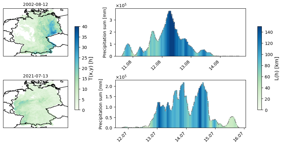
Figure 3 Characteristic time T(x,y) (left) and precipitation sum with colour indicating the characteristic length L(t) (right). Shown are the two precipitation events August 2002 (upper row; based on data from 10 August 2002 16:00 UTC to 14 August 2002 17:00 UTC) and July 2021 (lower row; based on data from 11 July 2021 20:00 UTC to 15 July 2021 21:00 UTC). The precipitation sum is calculated as the total sum of precipitation amount over the respective time period and across Germany.

Figure 3 shows the characteristic length and characteristic time as derived from one- and two-dimensional WT. The one-dimensional WT is computed at each grid point, while the two-dimensional WT is applied at each time step, providing spatially and temporally resolved estimates of the characteristic scales. The characteristic times and lengths that emerge as dominant in this representation are also found in the wavelet spectrum in Fig. 4. However, this representation additionally provides insight into when and where particular scale contributions occur. Both characteristic length and time reach their maximum near the centre of the event, with smaller-scale structures surrounding the main event in space and time. On average, the August 2002 event exhibits larger characteristic times (10.5 h) and lengths (82 km) compared to the July 2021 event (7.5 h and 74 km, respectively), indicating that the July 2021 event was, on average, more small-scale in nature.

Figure 4 Wavelet spectrum (Eq. 9) of the top six precipitation events identified Sect. 3. The lightgray, gray and black solid lines denote a characteristic speed of 5, 10 and 20 km h⁻¹. The centre of mass (Eq. 10) is indicated by a gray dot.

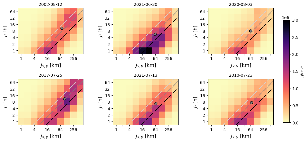
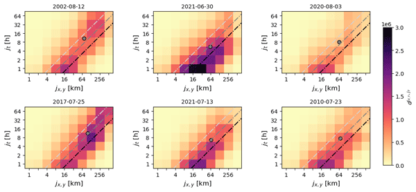
These insights from one- and two-dimensional WT, while interesting, do not fully represent the structure of an event because time and space are treated separately. To overcome this, three-dimensional approaches are required, allowing for a joint analysis of spatial and temporal scales. Figure 4 shows the spectral energies $e^{j_{XY},j_T}$ (Eq. 9) of the six most intense precipitation events, including the August 2002 and July 2021 cases. Each event shows different characteristics in terms of their space-time characteristics, reflecting how different individual precipitation events can be. Each panel displays the spectral energy of the corresponding event, decomposed into 10 spatial scales (j_XY) and 7 temporal scales (j_T). The sum over all scales equals the total spectral energy, which corresponds to the variance of the precipitation field. This representation illustrates how the spectral energy of each event is distributed across discrete combinations of spatial and temporal scales. The patterns observed here are consistent with our findings from Fig. 3.

Compared to the other events within the top six, the August 2002 event consistently shows a high proportion of energy at larger scales, together with the July 2017 event, which also displays substantial contributions at comparatively large scales – reaching up to approximately 256 km and 34 h in 2002, and up to 500 km and 64 h in 2017. The events from 2010, and 2021 exhibit comparatively stronger energy contributions at smaller scales. These observations are consistent with previous studies as detailed above.

A prominent and recurring feature across all spectra is the concentration of energy along a straight line with an approximate slope of one. This can be attributed to the movement of precipitation systems through space, as can be shown from the definition of characteristic speed ($U=L/T$). In the logarithmic presentation, this can be rewritten as $\log T=\log L-\log U$ (Kraus, 2004). Accordingly, the y-intercept gives an estimate of the characteristic speed and the magnitude of the energy along this line reflects underlying space and time scales. For reference, we included lines indicating a characteristic speed of 5, 10 and 20 km h⁻¹ in Fig. 4. Precipitation events can exhibit distinct characteristic velocities across spatial and temporal scales. For instance, in the August 2002 event we find from Fig. 4 that small-scale features tend to propagate faster than large-scale components, as indicated by the orientation of spectral energies for different sized features, highlighting the complex, multiscale dynamics of precipitation systems.

Table 1 Summary of mean spatiotemporal characteristics of the top six precipitation events identified Sect. 3. We report the characteristic length L, the characteristic time T (Eq. 10), the characteristic speed V and characteristic scale S (Eq. 11) for each event.

Finally, Table 1 summarises the characteristic properties of the top six precipitation events. For each event, we report the characteristic length L and time T (see Eq. 10), as well as the characteristic speed V and scale S (see Eq. 11). These metrics provide a concise representation of the spatial and temporal characteristics inferred from the spectral energy distributions in Fig. 4. For example, the comparatively large-scale nature of the August 2002 and July 2017 events is clearly reflected, and both are found to propagate relatively slowly. By contrast, the June 2021 event exhibits the smallest spatiotemporal scales and the highest propagation speed, followed by the flooding event in July 2021. The August 2020 and June 2010 events fall in between these two categories.

In comparison to the top 100 precipitation events analysed in the following section, the top six events are characterized by comparatively large characteristic scales and low characteristic speeds (see Fig. 5). This tendency toward larger-scale, slower-moving systems among the most extreme events is discussed in more detail below.

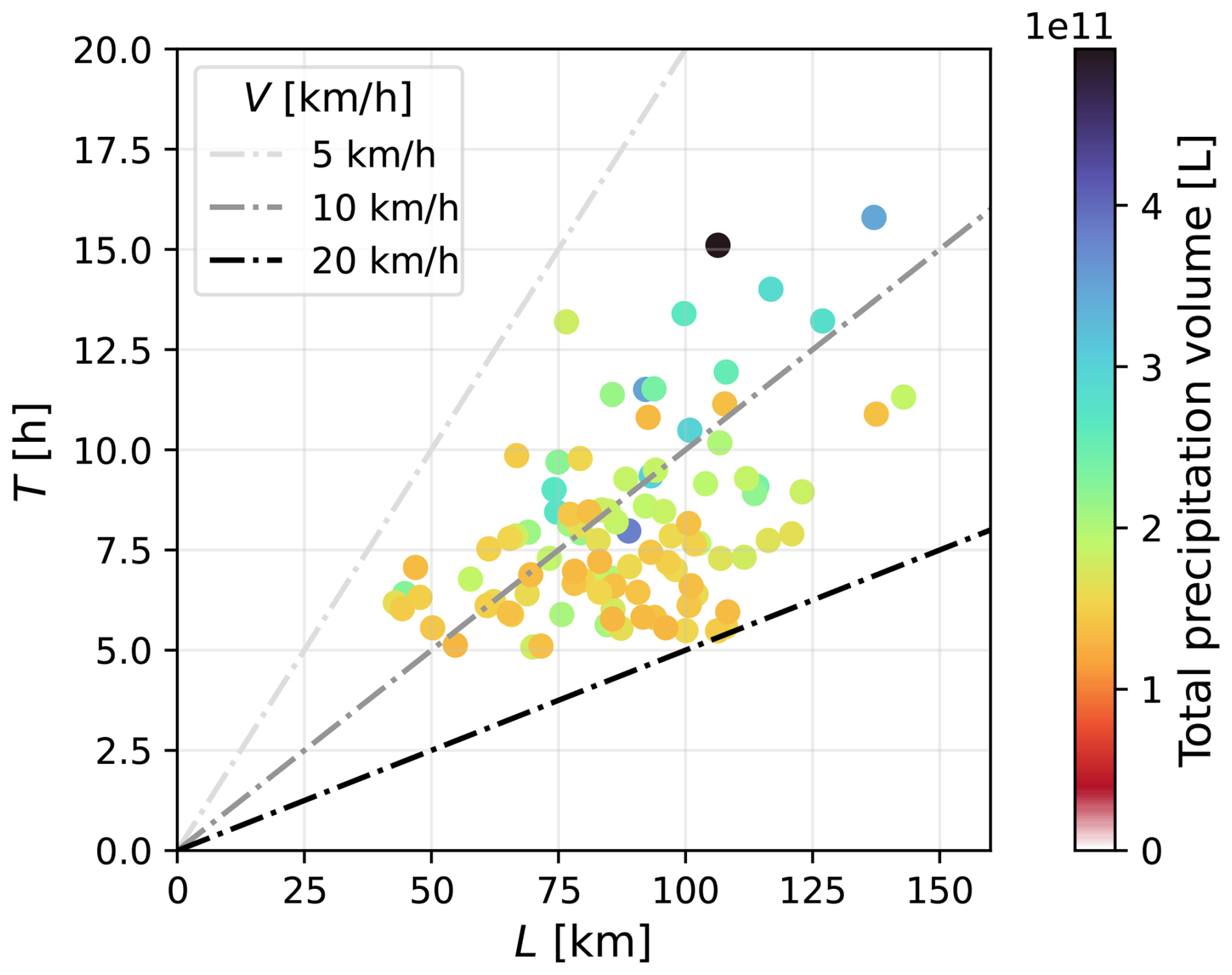
Figure 5 Scatter plot of the characteristic length L and characteristic time T (Eq. 10), for the top 100 precipitation events identified in Sect. 3. Point colour indicates total precipitation volume similar to Fig. 2. Straight lines indicate a characteristic speed V of 5 km h⁻¹ (light gray), 10 km h⁻¹ (gray) and 20 km h⁻¹ (black).

4.2 Statistical Analysis

After concluding from Sect. 4.1 that the characteristic properties provide a suitable representation of the spatiotemporal structure of a precipitation event, we now extend the analysis to a stochastic assessment of the top 100 events using characteristic length, time, speed and scale. Figure 5 summarises the characteristic length and characteristic time of the 100 most extreme precipitation events identified in Sect. 3. The events span a wide range of scales, with characteristic lengths between 43 and 143 km and characteristic durations between 5 and 16 h. The corresponding propagation speeds range from 5 to 20 km h⁻¹, which is physically plausible for precipitation systems. We further observe a tendency for high-volume precipitation events to be more slowly propagating systems, which – consistent with physical intuition – would come with their enhanced persistence. This feature will be examined in more detail in the following.

To further investigate the dominant spatiotemporal characteristics of the top 100 precipitation events, we apply a K-means clustering algorithm to the spectral energies $e^{j_{XY},j_T}$ (Eq. 9). We apply K-means clustering because it is widely used and provides interpretable results. Tests with alternative clustering techniques yielded consistent results and did not modify the findings presented below. To emphasize structural patterns rather than the absolute energies of each event, the spectral energies are normalized individually as: $e^{j_{XY},j_T}/\sum e^{j_{XY},j_T}$. We assess the quality of the cluster solution using the silhouette score (Rousseeuw, 1987) and evaluate stability under resampling with the adjusted Rand index (Hubert and Arabie, 1985) for K-means solutions ranging from 2 to 10 clusters (see Appendix Sect. A for full results). The highest silhouette score (0.31) and robust stability (median ARI = 0.80) are achieved for a three-cluster solution, which we adopt for the subsequent analysis.

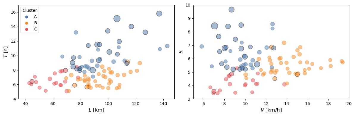
Figure 6 Scatter plot of (left) characteristic length L and characteristic time T (Eq. 10), and (right) characteristic speed V and characteristic scale S (Eq. 11). Shown are the top 100 precipitation events identified in Sect. 3. The point size indicates total precipitation volume similar to Fig. 2. The top 25 events are highlighted with black edge colour. The point colour indicates the cluster membership obtained from K-means clustering, which is applied to the normalized wavelet spectra $e^{j_{XY},j_T}/\sum e^{j_{XY},j_T}$.

In Fig. 6 (left), we show the characteristic length and characteristic time of each event, with colours indicating the assigned cluster. The three-cluster solution differentiates events as follows: (A) large spatiotemporal-scale events with low propagation speeds, likely associated with synoptic, quasi-stationary systems such as blocked cyclones or persistent frontal zones; (B) large spatiotemporal-scale events with substantially higher propagation speeds, likely dominated by strong large-scale advection, for example rapidly moving frontal systems or cyclones embedded in a strong westerly flow; and (C) small spatiotemporal-scale events that are likely associated with convectively driven precipitation This analysis suggests that spatiotemporal precipitation extremes are primarily governed by two features: Their characteristic speed V and a combined space–time magnitude, the characteristic scale S. Both quantities have been introduced in Sect. 2.2. In Fig. 6 (right), we display S and V for the top 100 events, clearly illustrating the differences between the three clusters with respect to these two variables. As already apparent in Fig. 5, high-volume precipitation events tend to propagate more slowly. This tendency is confirmed in Fig. 6, where we find that the top 25 events predominantly fall into cluster A. Although no formal statistical test was conducted, this observation is consistent with the physical interpretation of cluster A and cluster B outlined above, where slower-moving, large-scale events tend to accumulate higher precipitation totals.

Table 2 Slope for the linear trend analysis illustrated in Fig. B1. p-value for slope ≠0 in brackets (t-test).

We further analysed if there is a trend towards changes in the spatiotemporal characteristics with time in the data. We tested for linear trends in the previously introduced characteristic parameters (L, T, V, S), as well as in the total precipitation volume and the annual number of identified events. The analysis was conducted for both, the full time series and separately for each cluster. We fitted a linear regression using maximum likelihood estimation and performed a t-test on the slope. The results are summarized in Table 2. Further details of the statistical test and graphical illustrations are provided in Appendix Sect. B. Overall, we do not find any trends that meet the significance threshold of 0.01, which is likely due to the relatively short length of the time series. For trend analyses, this period is already quite short, so it is not surprising that statistically robust trends are absent. We do find indications of a decrease in the characteristic velocity of small-scale events (cluster C), but with a p-value of exactly 0.05, this result cannot be considered statistically significant. A longer observation period will be necessary to obtain more conclusive evidence in this regard.

5 Physical foundations

In a final step, we aim to quantify the characteristic properties using the additional data source ERA5. The characteristic variables L, T, V, and S are aggregated quantities. They are derived from precipitation over the 4 d window over Germany described in Sect. 3.2, and the information contained in the wavelet spectra is further condensed into a single characteristic spatial and temporal scale. Therefore, our analysis is not designed to resolve convective-scale processes. Instead, we aim to assess whether the proposed characteristic variables are consistent with the large-scale atmospheric dynamics governing precipitation events. Specifically, we consider the mean wind speed and the convective timescale. The convective timescale (τ_c; Done et al., 2006) quantifies the characteristic time over which atmospheric instability, expressed as CAPE, is removed by convective heating and thus serves as an indicator of convective activity. As mentioned above, larger (smaller) values of τ_c correspond to weaker (stronger) large-scale forcing. Importantly, both variables originate from reanalysis data (Sect. 3) and are not derived from precipitation fields. Instead, they serve as descriptors of the prevailing atmospheric conditions during each event. Taken together, these two variables provide a description of the prevailing atmospheric conditions during each event. This allows us to examine whether the characteristics inferred from precipitation events in the previous section, namely the characteristic scale and characteristic speed, align with the expected atmospheric influences.

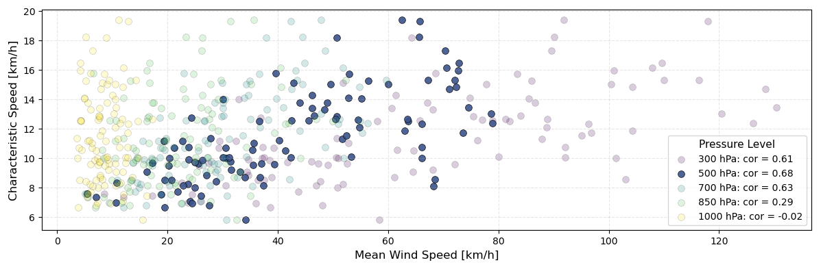
Figure 7 Scatter plot of the characteristic speed derived from the WT vs. the mean wind speed from ERA5 reanalysis at pressure levels of 300, 500, 700, 850, and 1000 hPa. Shown are the top 100 precipitation events identified in Sect. 3. Pearson correlations between characteristic and mean wind speeds are shown in the colorbar labels.

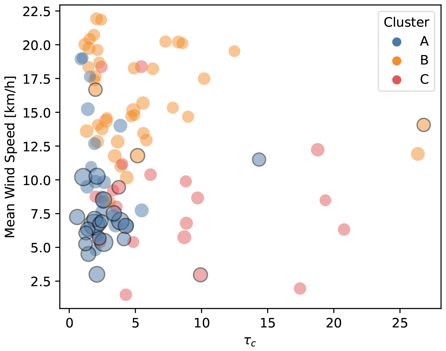
In Fig. 7, we compare the characteristic speeds derived from the wavelet spectrum with mean wind speeds from ERA5 reanalysis data over Germany during the respective events. The range of characteristic speeds falls well within the typical variability of synoptic-scale surface wind velocities, but the correlation is near zero. We however observe strong correlations (r>0.6) with the mean wind speeds of the higher levels between 300 and 700 hPa. The maximum correlations (r=0.68) are at 500 hPa, indicating a dynamical linkage between the propagation of the observed precipitation systems and the mid-tropospheric flow. This finding is consistent with the well-established association between midlatitude cyclone activity, frontal passages, and precipitation documented in synoptic meteorology (Bott, 2016; Hofstätter et al., 2018). Precipitation systems, especially those at the synoptic level, are propagated by the prevailing tropospheric flow rather than surface winds, where friction effects are minimal and winds reflect the geostrophically balanced motion of the atmosphere. As shown in Appendix Fig. C1, the classification still performs remarkably well when precipitation events are separated into their K-means clusters, as identified in Sect. 4.2, using the two independent variables τ_c and v_500 hPa. We thus conclude that the characteristic speeds and scales derived from our method are physically meaningful and align with expected atmospheric dynamics.

Figure 8 presents the Pearson correlation matrix of all characteristic quantities introduced in this study – the characteristic scale S, speed V, length L, and time T – together with the total precipitation volume, the convective timescale τ_c, and the mean wind speed at 500 hPa. The latter level was selected because it showed the strongest correlation in the previous analysis compared to 1000, 750, and 250 hPa. The correlations among the characteristic quantities summarize the findings from the previous sections. As expected, L and T show strong positive correlations with S, while S, T, and V are mutually related, reflecting the internal consistency of these measures. In contrast, S and V are almost uncorrelated, confirming that the characteristic scale and speed represent independent aspects of precipitation system behaviour.

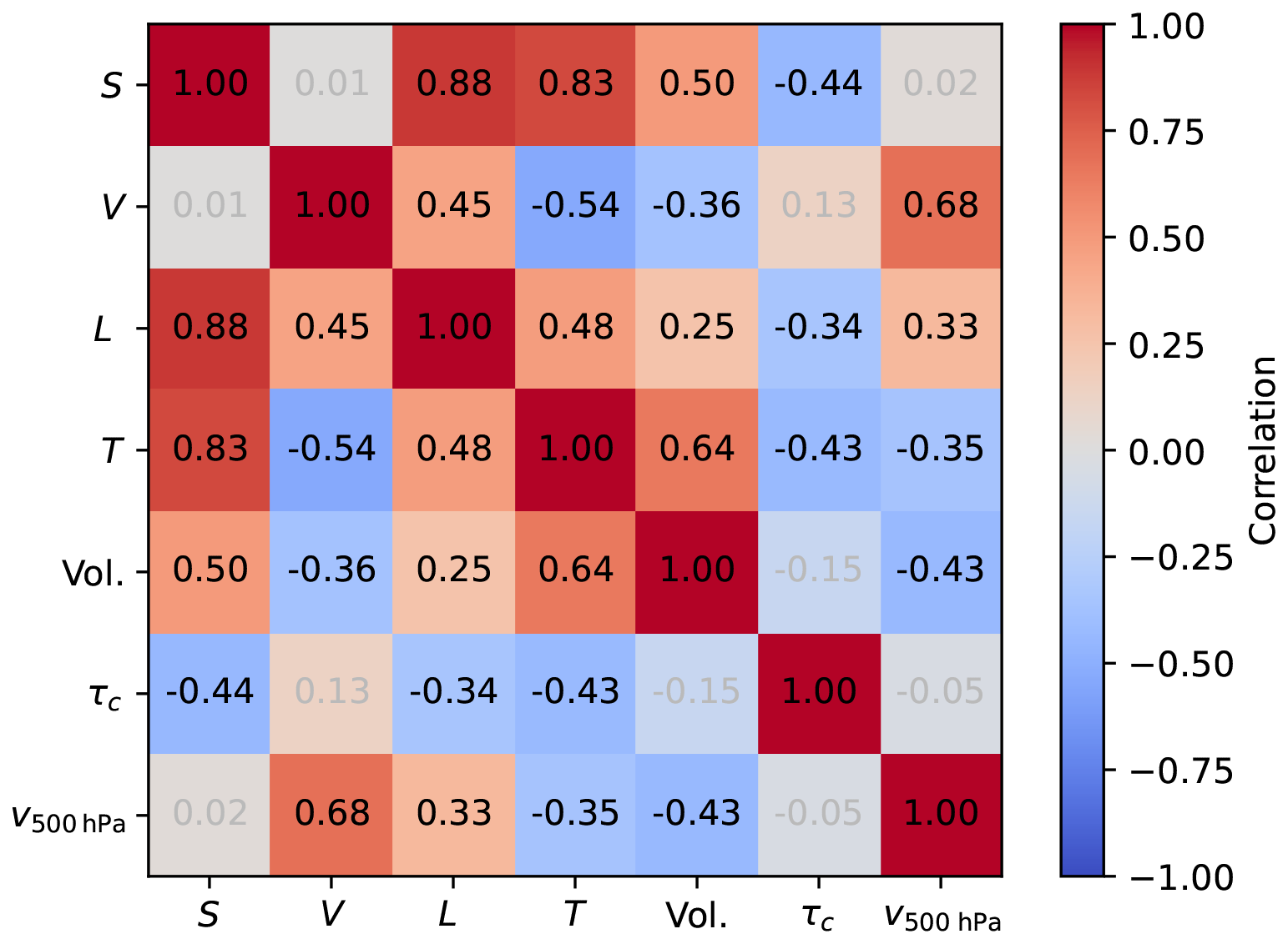
Figure 8 Pearson correlations between WT-derived characteristics (S, V, L, T), precipitation volume, convective timescale τ_c and mean wind speed in 500 hPa. Grey numbers indicate non-significant correlations at p=0.05 assessed with a permutation test (1000 permutations).

The total precipitation volume correlates positively with S and negatively with V, Although the correlations are not strong, this is consistent with the results in Sect. 4.2 suggesting that slow-moving, large-scale systems tend to produce greater accumulated precipitation amounts. Nevertheless, exceptions to this general tendency do occur, as smaller-scale or faster-moving systems can also generate substantial precipitation totals under favourable dynamic or thermodynamic conditions. We also find positive correlations between characteristic speed V and mean wind speed at 500 hPa, as shown previously, linking precipitation system propagation to mid-tropospheric flow.

Finally, the convective timescale τ_c correlates negatively with the S, suggesting that short τ_c – that is, strong large-scale forcing – tends to promote more extensive, large-scale precipitation systems, whereas longer τ_c values favour smaller, more localized convective systems. Note that τ_c represents the atmospheric adjustment or CAPE consumption timescale, while T denotes the duration of the precipitation system itself; hence, the two are expected to be negatively correlated.

6 Summary & Conclusions

We investigated the spatiotemporal characteristics of extreme precipitation events over Germany using WT. The WT is a spectral filtering method that decomposes the total energy of a signal into contributions from different scales or sizes. Our analysis considered three dimensions: two spatial and one temporal. However, we distinguished only between a combined spatial scale in the x- and y-directions and the temporal scale of precipitation events. Although a further separation of the two space dimensions is possible, a single spatial scale is consistent with the established scale-based view of the climate system (Kraus, 2004).

We identified precipitation events in the northern hemispheric summer months across Germany based on their total accumulated precipitation within a confined spatial and temporal window. This allowed us to capture events with a strong potential for hydrological and societal impacts, for example when they occur over river catchments or in areas with limited runoff capacity.

In fact, the top six events that we identified include several well-documented cases previously studied in the literature (Ulbrich et al., 2003; Ludwig et al., 2023), which confirms that our selection criterion is appropriate for identifying high-impact precipitation events. They also span a broad range of spatial and temporal scales, offering a solid basis for demonstrating the capabilities of our method. Using the six most intense precipitation events as illustrative examples, we demonstrated how our three-dimensional WT framework, namely the derived wavelet spectrum reveals contributions from different spatial and temporal scales within precipitation events. To the best of our knowledge, no comparable approach currently exists that enables an equally effective and scale-resolved decomposition. We conclude that the wavelet spectrum is particularly suited for analysing individual events. Possible applications include comparing specific precipitation events or how they are represented in different data sets.

To move from a detailed analysis of individual events to a broader examination of the top 100 events in Sect. 4.2, we summarized the mean spatiotemporal characteristics of each event. Again following the simplified concept illustrated by Kraus (2004), we provided a characteristic length L, a characteristic time T, a characteristic speed V and a combined spatiotemporal magnitude, which we denote as the characteristic scale S for each event. Using the top six events as an example, we demonstrated the suitability of this approach. By introducing S together with the characteristic speed V, we propose a new representation of the spatiotemporal characteristics of precipitation events. We see that the two quantities are only weakly correlated in our dataset (Fig. 8), despite both being deterministic functions of L and T. Any pair of variables among L, T, V, and S provides a complete description of the events, as they are derived from the same quantities. The choice of representation is therefore not unique, but depends on the desired interpretation. In our case, the weak correlation between S and V indicates that they capture complementary aspects of the event characteristics and provide a compact and non-redundant statistical representation.

Extending our analysis to the top 100 precipitation events, we applied statistical clustering to the wavelet spectra. In doing so, we aimed to identify distinct patterns and structures in the spatiotemporal characteristics of precipitation extremes. Our analysis revealed two key parameters: the characteristic scale, and the characteristic speed. The pronounced dominance of the characteristic scale and propagation speed is likely linked to the mid-latitude focus region, which is governed by prevailing westerlies and the associated advection of precipitation systems. The importance of the spatial scale further reflects the substantial heterogeneity of precipitation structures in this region, arising from the coexistence of different underlying mechanisms, such as convective and synoptic-scale processes.

Most of the 25 strongest events, measured by their total precipitation within a confined area and time period, are characterized by relatively slow characteristic speeds and large characteristic scales. This relationship becomes even clearer when considering the correlations between these variables. We therefore conclude that the spatiotemporal characteristics of precipitation events are of fundamental importance. Approaches such as the one proposed in this study can substantially advance our understanding of precipitation processes and their response to climate change. While we did not find significant changes in these characteristics over the observational period – likely due to the limited length of the available time series – studies based on climate model simulations already indicate potential changes in extreme precipitation events under future climate conditions (see Hundhausen et al., 2024).

In a final step, we correlated the characteristic variables of precipitation events with variables describing atmospheric dynamics. We find that the characteristic speed is correlated with the mean wind speed at 500 hPa. Furthermore, by means of the convective time scale, we linked large-scale precipitation events to large-scale atmospheric processes. These results confirm the physical plausibility of our analysis and highlight its suitability for establishing quantitative links between precipitation events and atmospheric dynamics.

The potentially large uncertainties in precipitation data should always be taken into account, particularly when comparing the spectral properties of precipitation from different data sources or even non-homogeneous observation systems. An impression of how large the differences are in the precipitation amounts of a single event can be seen in Kracheletz et al. (2025), who compared different observations and reanalyses. In addition, the spatial error structure of radar data is very inhomogeneous due to the radial observation method, although radar data is probably the best data we have to assess spatial properties. Different spatial interpolation methods also influence the spatial structure of the data and contain little information about the actual spatial dependency structure. Therefore, gridded data based on station data are unsuitable for such an analysis. In reanalyses and models, the spatial structure is determined by the effective resolution of the models, which is usually much coarser than the grid spacing (Bierdel et al., 2012). The uncertainties in the spectral characteristics of the data is similarly large as in the respective gridded version, since wavelet transformation represents a linear transformation, and the calculation of the spectral characteristics only provide some averaging over space. One should therefore treat these spectral characteristics similar to other measures in data analysis, with a thorough assessment of statistical significance (Torrence and Compo, 1998).

The derived characteristics establish a direct link to classical classifications of atmospheric scales (e.g., Kraus, 2004; Thunis and Bornstein, 1996). While the present study focuses on precipitation, the same methodology can also be applied to other atmospheric variables such as wind or pressure, enabling a scale-sensitive characterization of a wide range of atmospheric processes.

In summary, the proposed characteristic variables constitute a robust and transferable tool for quantifying the mean spatiotemporal properties of precipitation events. They are particularly well suited for the systematic analysis and comparison of multiple events, and allow for consistent comparisons across different datasets or scenarios. Our scale-aware analysis of precipitation events can further provide new insights into the underlying processes, which operate across a range of spatial and temporal scales. A more comprehensive assessment, including convection-permitting climate model simulations, is planned for future work.

Appendix A: Assessment of K-means Cluster Size

To evaluate the quality and robustness of the K-means clustering results, we adopt a twofold validation approach. Cluster quality is assessed using the silhouette score (cf. Rousseeuw, 1987), while stability under sampling variability is evaluated via the adjusted Rand index (ARI; Hubert and Arabie, 1985). Figure A1 shows the silhouette scores for cluster sizes ranging from 2 to 10. The silhouette score measures how well each data point fits within its assigned cluster compared to other clusters, with values ranging from −1 (poor fit) to 1 (clear separation). We find a maximum score of 0.31 for a three-cluster solution, indicating a moderate but meaningful cluster structure. Based on this result, we proceed with three clusters in the subsequent analysis. To evaluate the robustness of this three-cluster solution, we generate 1000 random subsamples, each containing 80 % of the top 100 events (sampled without replacement). A subsample size of 80 % was chosen to ensure that the main characteristics of the event set are preserved while allowing for meaningful perturbations of the sample composition. Tests with alternative subsample sizes (not shown) yielded qualitatively similar results. For each subsample, we compute both the ARI and silhouette score. The distribution of these scores is shown as box plots in Fig. A1. The silhouette scores show a stable distribution centred around the observed value, with only a few isolated outliers (median=0.30). The ARI further indicates a high degree of structural stability across subsamples, with a median value of 0.80. Taken together, these results suggest that the clustering solution provides both consistent inter-cluster separation and robust cluster assignment with respect to sampling variability.

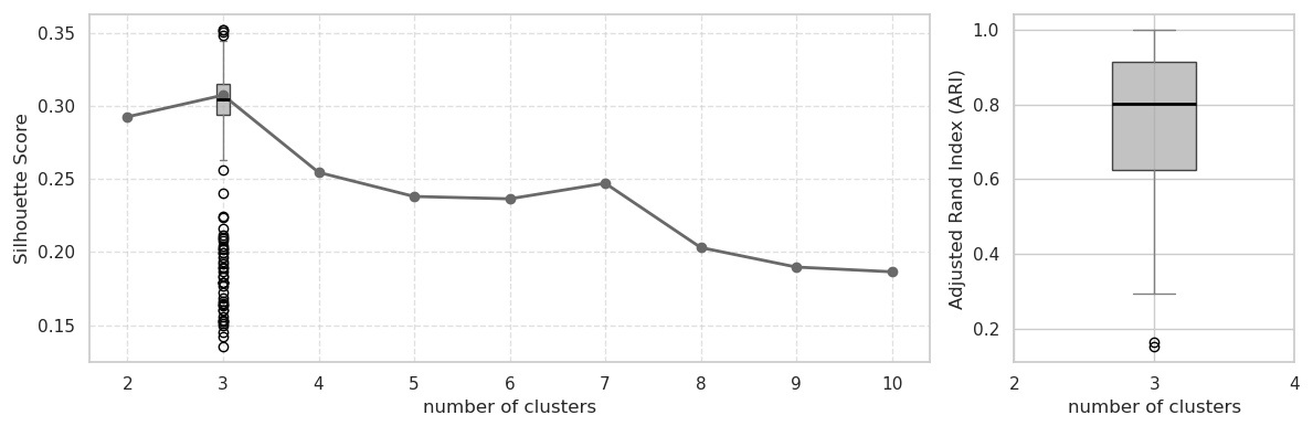
Figure A1 Silhouette score (left) and Adjusted Rand Index (ARI, right) for K-means clustering of the wavelet spectra of the top 100 precipitation events identified in Sect. 3. The silhouette score is shown for cluster sizes ranging from k=2, …, k=10. The boxplots are based on a fixed number of three clusters and represent the distribution of silhouette scores and ARI values calculated from 1000 random subsamples (each comprising 80 % of original data).

Appendix B: Testing for changes through time

In this paper, we analyse precipitation data from a total of 24 years. This naturally raises the question of whether we can find evidence of changes over time. In Sect. 4.2 we therefore present the results of a statistical testing of linear trends. We examine the key characteristics as introduced in this paper, namely length, time, speed, scale, total precipitation volume and, additionally number of events per year within the top 100. Figure B1 illustrates these six variables with time. The significance testing was performed using the integrated Wald test in the sciPy Python function lineregress, whose null hypothesis is that the slope is zero.

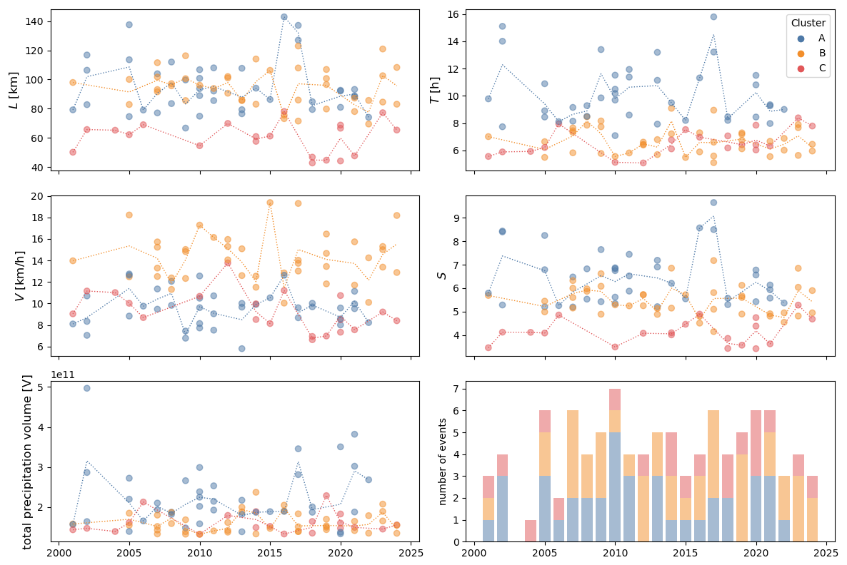
Figure B1 Scatter plots of the characteristic length L, characteristic time T, characteristic speed V, characteristic scale S, total precipitation volume (similar to Fig. 2) and number of events for each year. Shown are the top 100 precipitation events identified in Sect. 3. The points are coloured according to cluster assignments obtained via K-means clustering similar to Fig. 6. Dotted lines indicate average values for each year and cluster.

Appendix C: Connections with atmospheric dynamics

In Fig. C1, we show the convective timescale τ_c calculated in Sect. 5 and the mean wind speeds at 500 hPa for the 100 heaviest precipitation events identified in Sect. 3. The colour coding highlights the three clusters as identified in Sect. 4.2. Since both variables reflect the state of the atmosphere during the precipitation event and are not derived from precipitation radar measurements, the classification into the three clusters works remarkably well. We therefore conclude in Sect. 5 that the characteristic speeds and scales derived from our method are physically meaningful and align with expected atmospheric dynamics.

Figure C1 Same as Fig. 6 but for convective timescale τ_c and mean wind speeds in 500 hPa.