Evaluation of AI-based seasonal weather ensembles as input for fluvial flood risk estimation: a case study over the Elbe basin

A key challenge in flood risk analysis is the construction of hazard events that are physically plausible yet extend beyond historical observations with appropriate frequency and spatial coherence. This is commonly addressed through large simulations of synthetic weather scenarios that sample low-likelihood, high-impact events beyond the observed record. Although popular in industrial risk-based workflows, traditional statistical approaches to synthetic weather generation can be limited in their ability to represent the full range of physically plausible variability and spatial structure.

Here, we demonstrate a framework that uses an AI-based weather model as a stochastic generator of event sets suitable for flood risk assessment. We adapt the huge ensembles (HENS) approach using a Spherical Fourier Neural Operator (SFNO)-based atmospheric model combined with a diagnostic precipitation model, forming a framework termed “PrecipHENS”. This framework produces more than 1000 synthetic European winter seasons of precipitation and temperature at 0.25° resolution, with modest computational cost (using NVIDIA Earth-2 stack, 112 GPU hours on NVIDIA L40s GPUs).

Using an Elbe River case study, we evaluate PrecipHENS against risk-relevant criteria, including reproduction of present-day climatology, preservation of spatial and temporal dependence, representation of extremes, and extrapolation beyond the historical record in event space. PrecipHENS reproduces key features of precipitation and temperature climatology, preserves spatial dependence, including the decay of extremal co-occurrence with distance, and generates a substantially broader diversity of extreme precipitation events than an industry-standard conditional multivariate extreme-value benchmark. Principal component analysis of extreme precipitation fields shows that PrecipHENS spans a much broader space of storm structures than the benchmark or the historical record, indicating it is able to produce previously unseen weather rather than repetition of past patterns.

To assess flood risk relevance, the AI-generated weather sequences are coupled with a hydrological model. The resulting river flow simulations are consistent with observed climatology and extreme discharge behaviour, demonstrating that meteorological realism translates into physically plausible hydrological response. Together, these results show that AI-based large-ensemble weather generation can support event set construction for flood hazard and flood risk applications. More broadly, this framework provides a pathway for expanding the physically plausible sample space in applications that require robust characterisation of extremes, including risk assessment, climate-impact analysis, and storyline development.

1 Introduction

Flooding is a complex and damaging natural hazard, with both pluvial (surface water) and fluvial (riverine) events contributing to substantial financial, environmental, and social costs (Svetlana et al., 2015; Allaire, 2018; Zhang et al., 2024). For example, CRESTA CLIX (2024) described 2024 as the “year of the flood”, with flood events responsible for 78 % of the USD 18.2 billion in insured losses from all non-US catastrophe events exceeding USD 1 billion. Robust estimation of flood risk is crucial for disaster preparedness, infrastructure planning, adaptation planning, and (re)insurance pricing and capital management (Mitchell-Wallace et al., 2017; Tyler et al., 2019; Ferreira et al., 2022; Lamb et al., 2022).

Despite its importance, flood risk estimation remains challenging. Floods are highly variable in space and time, due to their dependence on multiscale processes (e.g. convective storms, frontal systems, persistent wet spells, snowmelt and antecedent moisture) that are shaped by complex interactions between meteorology and hydrology. Observational records are often short and incomplete, rarely containing enough independent extreme events to robustly characterise the tail of flood-relevant drivers that dominate expected annual losses at the spatial scales required for risk modelling. In particular, limited record length constrains our ability to observe and quantify regionally coherent, low-frequency precipitation patterns that can dominate portfolio-scale flood losses.

1.1 Stochastic event sets for risk estimation

To address limitations in available data, flood risk estimation often relies on simulation-based approaches that generate large sets of synthetic but physically plausible weather scenarios, extending the effective sample of hydrometeorological extremes. In catastrophe models, which are particularly used in the (re)insurance industries, these stochastic “event sets” underpin probabilistic estimates of losses from pluvial and fluvial flooding (Mitchell-Wallace et al., 2017). Each event set comprises spatially and temporally coherent weather and hydrological patterns, typically precipitation fields for pluvial flooding and river flow simulations for fluvial flooding, that together represent the diversity of potential flood events. This allows tail risk estimation beyond what can be inferred directly from the historical record under assumptions of a stationary present-day climatology, which is typical for many operational catastrophe models.

Two broad classes of approaches dominate event set construction, each with important limitations for flood risk analysis. Physics-based models are one such approach, such as numerical weather prediction (NWP) and/or climate models coupled to hydrological models, which may be nested to achieve the required spatial scales for flood impact analysis (Cotterill et al., 2024; Kay et al., 2018; Schaller et al., 2016). Such approaches allow exploration of rare events beyond the observed record, that remain physically consistent across multivariate fields (including precipitation, temperature, wind) and over large spatial and temporal domains. However, they remain computationally expensive, making it difficult to produce the very large ensembles needed for robust estimation of tail risk, particularly at the spatial resolution required for the flood impact modelling.

The second broad class of approaches employs statistical techniques based on parametric multivariate extreme-value models that have been trained on observed or reanalysis data (Keef et al., 2013). These methods can reproduce observed marginal behaviour and dependence structures for extremes while remaining computationally efficient, and they can be tailored to reproduce features of extremes that matter for the hazard of interest, such as clustering of events to model persistence of wet spells. However, they may provide limited representation of underlying physical dynamics and can be sensitive to modelling assumptions, including the limited historical record used for training. Therefore, they may overfit and not necessarily cover the entire sample space of plausible spatial weather patterns. As a result, while statistical generators can be highly effective for certain risk metrics, they may not always provide a complete substitute for physically coherent weather sequences due to lack of generalisability.

1.2 AI weather models as an emerging opportunity

A rapidly developing third class of approaches, AI-based weather models, offers a potential pathway to bridge aspects of the trade-offs between classical physics-based models and statistical techniques. Modern machine learning (ML) weather models can emulate key components of atmospheric dynamics and generate gridded meteorological fields at low computational cost, enabling very large ensembles and long rollouts that would be expensive with traditional dynamical models (Mahesh et al., 2025). The broad landscape includes deterministic surrogates/emulators, probabilistic and ensemble models. In principle, these methods offer the potential to generate ensembles large enough for tail-risk estimation, while maintaining regional-scale spatial coherence and multivariate consistency (e.g. precipitation and temperature) required for hydrological modelling, all whilst remaining computationally tractable for industrial workflows.

The driving use-case behind the development of AI-based weather models has been medium-range and sub-seasonal forecasting, and thus evaluation focusses on metrics associated with such (Ben Bouallègue et al., 2024; Rasp et al., 2020). However, an accurate forecasting model does not guarantee suitability for flood risk applications. Many ML systems are trained to minimise average error (e.g. mean squared error), which can encourage reproduction of typical conditions (e.g. general climatology) rather than the full distributional variability relevant for extremes (Mahesh et al., 2025; Xu et al., 2024). Recent work suggests that specific architectures and training strategies can better preserve variability and support stable long rollouts, including operator-learning models such as the Spherical Fourier Neural Operator (SFNO; Bonev et al., 2023) and specific retraining strategies focussing on extreme representation (Mahesh et al., 2024, 2025). Such models are able to capture seasonal cycles, making them well suited for (sub)seasonal use cases (Karlbauer et al., 2024; Peings et al., 2026). These developments motivate the question of whether AI-based weather models can be used as a stochastic generator capable of producing event sets for hazard and risk assessment, in addition to the primary use case of prediction.

1.3 Suitability of AI weather models for flood risk estimation

For flood risk estimation, a central requirement is the representation of spatially coherent storms across regional scales, where the joint behaviour of precipitation over large areas drives both pluvial losses (through spatial clustering of intense rainfall) and fluvial impacts (through catchment-integrated rainfall, antecedent wetness, and temperature-mediated processes such as snow accumulation and melt). Against these flood risk-specific requirements, it remains unclear whether AI-based weather models can satisfy the conditions needed for present-day flood risk estimation, where the aggregation of events across space, time, and ensembles is key. In particular, open questions remain regarding their ability to reproduce unbiased present-day climatology and seasonality relevant for hydrological response, preserve spatiotemporal dependence structures that control regional aggregation of flood losses, exhibit credible statistical tail behaviour for flood-generating extremes, and extrapolate beyond the historical record in event space.

To address this gap, we evaluate AI-generated weather sequences explicitly through a flood risk lens. We introduce a set of goals that define minimum “fit-for-purpose” requirements for event set inputs: (G1) reproduce observed present-day distributions relevant for flood processes; (G2) preserve credible spatial and temporal dependence; (G3) exhibit credible statistical tail behaviour for extreme precipitation and ensuing hydrological response; and (G4) demonstrate robustness and generalisability beyond the historical record. We apply these criteria first to precipitation fields and then to hydrologically relevant outcomes by converting simulated meteorology into river flows using a conceptual hydrological model. This two-stage evaluation reflects how event sets are used in practice: meteorological realism must translate into credible hydrological hazard. This study therefore addresses a methodological gap at the interface of AI weather modelling and flood risk estimation: evaluating whether AI-generated seasonal ensembles can function as inputs to credible event sets when judged against risk-relevant, rather than forecast-oriented, criteria.

1.4 Scope and contributions

This study provides a proof-of-concept assessment of AI weather generation for flood risk event sets under present-day conditions (1980–2024), without attempting to model future climate change. Specifically, we:

1. Propose an evaluation framework that can be reused to test AI weather generators for catastrophe risk applications;

2. Evaluate seasonal ensembles from an AI weather model (SFNO-based) against risk-relevant criteria (G1–G4);

3. Assess hydrological implications by translating meteorological sequences into river flow simulations and re-evaluating performance against the risk-relevant criteria (G1–G4);

4. Benchmark AI-generated precipitation against an established industry approach grounded in multivariate extreme-value theory (Keef et al., 2013).

Together, these contributions provide the first systematic assessment of AI-generated weather ensembles for flood risk event set construction. We emphasise that this study presents a framework rather than an optimised operational product. Our aim is to demonstrate the potential of AI weather models to generate seasonal-scale precipitation and temperature fields suitable for flood risk estimation, rather than to provide a definitive or fully calibrated dataset.

1.5 Outline of the paper

Section 2 details the data and methods, including the SFNO-based framework (Mahesh et al., 2024, 2025) and our benchmark. The results in Sect. 3 first assess generated precipitation against G1–G4 over a large European river basin and includes the comparison of the SFNO data to the statistical benchmark, before presenting a method to translate the AI-based sequences into river flow and evaluating these against G1–G4. We conclude in Sect. 4 with a discussion of the broader implications of this proof-of-concept study for the flood risk industry.

2 Data and methods

This section describes the methodology used to generate and evaluate seasonal weather ensembles for flood risk event set generation. The AI-based weather generation framework used in this study combines an atmospheric model deployed within a large-ensemble configuration with a diagnostic precipitation model and is hereafter referred to as PrecipHENS. Section 2.1 provides an overview of PrecipHENS. Section 2.2 then describes the methodology used in this study to generate seasonal weather ensembles, followed by Sect. 2.3, which details the datasets used for model initialisation. Section 2.4 describes the hydrological simulation approach used to assess the river flow response produced by the PrecipHENS ensembles, while Sect. 2.5 presents a comparative precipitation modelling framework, referred to as the benchmark, which we use to contextualise evaluation of the AI-generated precipitation fields.

2.1 Overview and evaluation framework of PrecipHENS

The PrecipHENS framework is used here as a stochastic weather generator rather than as a predictive forecasting system, with the aim of producing large, physically plausible seasonal ensembles of precipitation and temperature that extend beyond the historical record and are suitable for downstream flood risk analysis.

PrecipHENS uses the huge ensembles (HENS) approach (Mahesh et al., 2024, 2025) to generate thousands of physically plausible atmospheric realisations. The integrations are intentionally extended beyond the period of skilful dependence on their initial atmospheric states, such that the resulting sequences are not predictive in the forecast sense. Instead, they are designed to support risk-based analyses by expanding the range and diversity of plausible weather conditions that can give rise to flooding across large river basins.

To evaluate whether PrecipHENS is fit for use in flood risk event set generation, we apply a structured set of evaluation criteria that reflect common requirements in probabilistic hazard modelling. Specifically, the generated ensembles are assessed against the following goals, as briefly introduced in Sect. 1:

• G1. Reproduction of present-day climatology, which involves reproducing key climatic features, such as long-term means and statistical distributions of variables like precipitation. As the aim of this work is to assess the risk of flooding under present-day conditions, the observed climatology that is referred to here is that of 1980–2024 and there is no scope in this work to provide a framework for modelling future climatology. This is particularly important for conceptual hydrological models, such as the model we will use later, which integrate water balances over time and are sensitive to biases in meteorological inputs.

• G2. Reproduction of spatial and temporal dependence, which requires that simulations reflect credible spatial and temporal dependencies. Inadequate representation leads to fragmented or overly smooth precipitation fields, distorting event sequencing and persistence. Coherence must be maintained both in typical variability and in rare events, which are especially relevant for catastrophe modelling where risk is aggregated across time (e.g., insurance terms) and space (e.g., national portfolios) (Lamb et al., 2010; Mitchell-Wallace et al., 2017). Event clustering and spatial structure matter both for long-term patterns (e.g. seasonal drivers) and short-term impacts (e.g. flooding across catchments) (Merz et al., 2014; Steirou et al., 2022).

• G3. Statistical tail behaviour of extreme events, which highlights the importance of simulating the frequency and magnitude of extremes. Under- or overestimating the tails of the distribution can respectively underplay or exaggerate risk. While global datasets such as the European Centre for Medium-Range Weather Forecasts (ECMWF) Reanalysis v5 (ERA5; Hersbach et al., 2020) offer useful historical context, their limited length challenges the estimated frequency of long return period events.

• G4. Robustness and generalisability beyond the historical record, which refers to the need for variability without overfitting and demonstrating controlled sensitivity to changes in input conditions. This is vital given the spatial heterogeneity of flood drivers; events are often locally unique due to terrain, land use, and hydrological conditions and thus generally not transferable to another location (Zanardo and Salinas, 2022).

2.2 AI-based seasonal weather ensemble generation (PrecipHENS)

This section describes the methodology used to generate seasonal weather ensembles using PrecipHENS. We first describe the general PrecipHENS set up followed by the configuration used in this study to produce a large winter ensemble.

2.2.1 The general PrecipHENS methodology

An overview of the PrecipHENS workflow is shown in Fig. 1, illustrating the integration of SFNO (Bonev et al., 2023) for atmospheric simulations with diagnostic precipitation generation via an Adaptive Fourier Neural Operator (AFNO)-based model (Pathak et al., 2022), along with the sources of initial condition and model ensemble variability considered in this study.

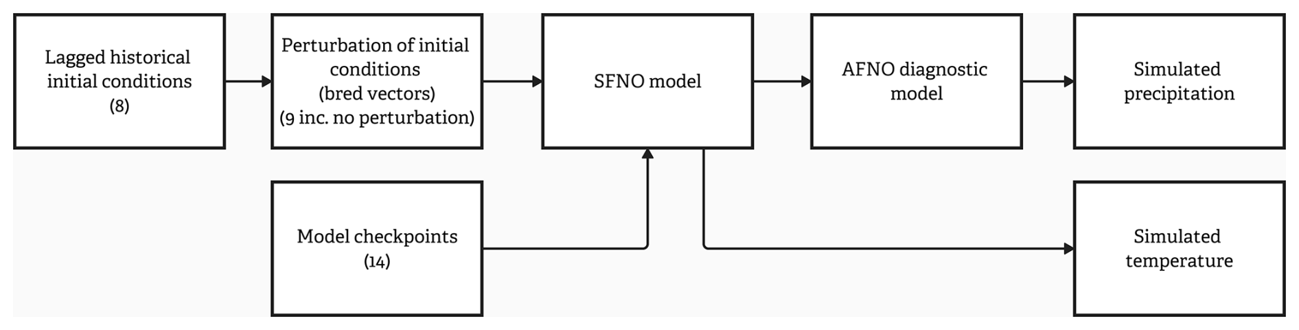
Figure 1 Schematic of PrecipHENS, the AI-powered approach to weather generation we develop in this study. Lagged historical initial conditions are perturbed using bred vectors and passed through multiple SFNO model checkpoints to represent initial condition and model uncertainty. The resulting SFNO forecast is then processed through an AFNO-based diagnostic model to generate simulated precipitation. For subsequent timesteps, the SFNO model is applied autoregressively, with its own previous forecast used as input to generate a continuous time series.

In PrecipHENS, ensemble generation follows the HENS methodology, in which uncertainty is sampled through use of both different initial condition and different model checkpoints (Mahesh et al., 2025). HENS accounts for initial condition uncertainty through a custom centred bred vector perturbation scheme (Mahesh et al., 2025; Toth and Kalnay, 1993, 1997). This scheme samples the fastest-growing modes of forecast error by iteratively breeding perturbations through the model dynamics, generating flow-dependent perturbations that maintain physically consistent structures across variables and levels.

The forecast model applied in HENS is a tailored version of SFNO (Bonev et al., 2023), a machine learning emulator of global numerical reanalyses, here trained on ERA5 from 1979–2015 (Hersbach et al., 2020). SFNO learns atmospheric evolution operators in spectral (spherical harmonic) space and enforces rotational equivariance, enabling representation of large-scale dynamics rather than memorising specific historical sequences (Bonev et al., 2023). For HENS, the architecture and the training methodology of SFNO have been configured for improved representation of extremes (Mahesh et al., 2025).

SFNO is a deterministic, global forecast model which predicts the atmospheric evolution at 6-hourly timesteps. The data generated by PrecipHENS consists of 74 surface and pressure level variables provided on a 0.25° horizontal grid and 13 vertical pressure levels. Because of the deterministic nature, SFNO lacks an inherent representation of model uncertainty. To approximate this, the developers of HENS trained multiple model “checkpoints” using identical training data and protocols but different random initial model weights, causing each checkpoint to converge to a distinct local minimum of the mean-squared-error loss surface used during training and so providing a diverse ensemble of plausible solutions.

As precipitation is not an output of the SFNO model, to complete the PrecipHENS workflow total accumulated precipitation is derived diagnostically from a subset of 20 atmospheric fields generated by SFNO using an AFNO-based precipitation model (Pathak et al., 2022). The diagnostic model is applied at each 6-hourly temporal timestep of the atmospheric simulations to estimate 6-hourly total precipitation. As with SFNO, the precipitation diagnostic has been trained using ERA5 data.

2.2.2 The PrecipHENS implementation for this evaluation study

For the present study, PrecipHENS is configured to generate a large ensemble of winter-season meteorological conditions (December–February). Ensemble simulations are initialised from a set of lagged atmospheric initial conditions drawn from mid-November, allowing sufficient lead time for simulations to evolve prior to the winter season of interest. The inclusion of an initial simulation period prior to December ensures that the winter-season sequences analysed here are not used as forecasts, but rather as independent, physically plausible realisations of present-day seasonal weather variability relevant for flood-risk analysis.

Ensemble diversity is achieved through the combination of three sources of variability: lagged initial conditions, initial condition perturbations and multiple trained model checkpoints (shown in Fig. 1). Eight atmospheric initial conditions are selected from ERA5 at 00:00 UTC on consecutive dates in mid-November (9–16 November 2023, inclusive). For each initial date, a set of nine initial atmospheric states is constructed, comprising of one unperturbed state and four pairs of positive and negative bred-vector perturbations. This results in 72 distinct initial states (8 initial dates × 9 perturbations). Each of these is then simulated using 14 of the independently trained SFNO model checkpoints from the HENS study, yielding a total ensemble size of 1008 members.

For the analyses presented in this study, all variables are aggregated to daily resolution, with each day defined using the 00:00 UTC time step. Precipitation is accumulated over each day, while temperature is averaged.

PrecipHENS was generated on NVIDIA L40s GPUs with a batch size of two members per GPU. The rollout for two ensemble members takes on average 13 min 20 s, i.e., requiring roughly 112 GPU hours to produce the full weather dataset. Initial conditions are typically generated in pairs using positive and negative perturbations of the same vector, but SFNO integrations are executed separately for each ensemble member, enabling parallelisation across the ensemble dimension during simulation. For this work, we employ Earth2Studio (PhysicsNeMo Contributors, 2024), a modular open-source Python framework that provides unified access to state-of-the-art AI weather models, widely used meteorological data sources and standard output formats. PrecipHENS builds upon the HENS reference workflow provided within Earth2Studio.

2.3 Data used for PrecipHENS and evaluation

2.3.1 Study region

While PrecipHENS is configured as a global weather-generation framework, focusing on a large, continental-scale river basin allows detailed evaluation within a large catchment representative of basin-scale flood risk processes. Applying the same continuous hydrological modelling framework globally would be computationally prohibitive and is beyond the scope of this proof-of-concept study.

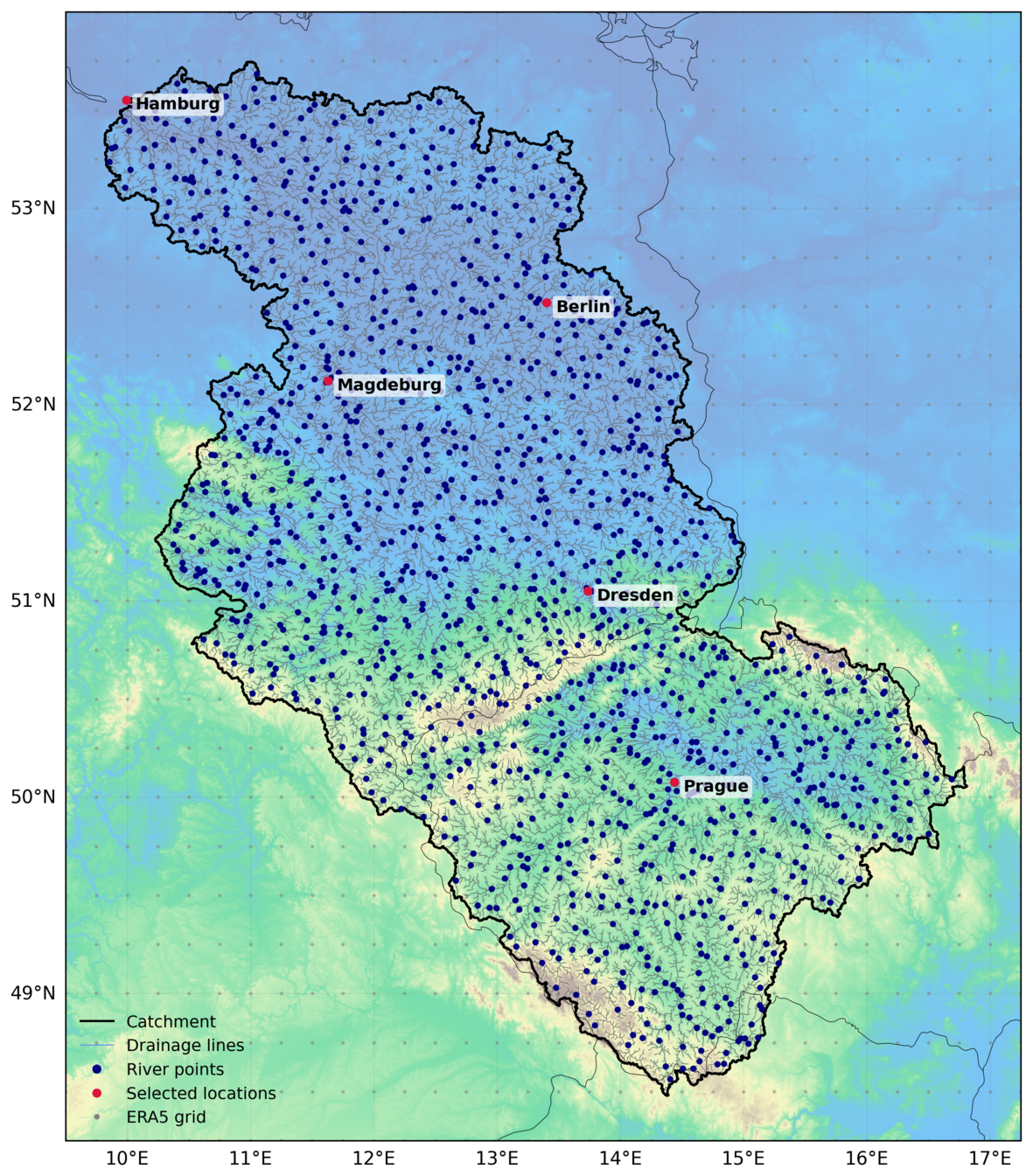
Figure 2 Overview map of the Elbe River basin showing the catchment outline (black), drainage lines (grey), river simulation points (blue), and the ERA5 reanalysis grid (light grey). Some selected major cities (red) are labelled for geographical reference. Terrain shading derived from the Copernicus GLO-30 Digital Surface Model highlights topographic variation across the region.

The analysis focuses on the Elbe river basin in Germany (shown in Fig. 2), a large European catchment that encompasses varied geomorphological conditions from the mountainous upper catchment in Czech Republic to its lowland floodplains in Germany. The Elbe is susceptible to basin-wide flooding, with the dominant flooding season being winter (Merz and Thieken, 2009), driven by prolonged precipitation and, in some regions, the interaction between rainfall and snowmelt (Nied et al., 2013).

The analysis is therefore restricted to contiguous three-month winter seasons. This period captures the dominant flood-generating processes while keeping individual simulations computationally tractable. From a risk modelling perspective, seasonal simulations are a natural unit for downstream event-set applications, where individual seasons can be resampled and combined to construct long synthetic records suitable for annual loss estimation.

2.3.2 Atmospheric reanalysis data

The ERA5 dataset (Hersbach et al., 2020) is used in three distinct roles throughout this study:

1. Initial conditions, ERA5 provides the atmospheric initial conditions for the PrecipHENS ensemble simulations (Sect. 2.2).

2. Historical reference, ERA5 is used as the primary dataset to represent the historical record in this study. ERA5 provides a physically consistent, multidecadal record of atmospheric conditions and is used as the reference dataset for precipitation and temperature analyses over the Elbe basin. Rather than using the native ERA5 precipitation product, we derive a historical reference precipitation dataset through the same diagnostic precipitation model applied to the PrecipHENS simulations to derive the historical reference precipitation dataset used throughout the analysis. All references to historical precipitation in this study therefore correspond to diagnostically derived ERA5 precipitation. This approach ensures that differences between datasets reflect the weather-generation methods rather than inconsistencies between precipitation products.

3. River flow response calibration, ERA5-derived precipitation and temperature provide the consistent meteorological forcing for calibration and application of the hydrological modelling, enabling evaluation of river flow response at the catchment outlets considered in this study (shown in Fig. 2).

All ERA5-based datasets are processed to daily temporal resolution over the Elbe basin for consistency with the subsequent precipitation evaluation and hydrological simulations.

2.4 Hydrological evaluation methodology

While precipitation simulations allow direct assessment of pluvial flooding, river flow is the key variable for fluvial risk. Given a weather simulation, a continuous hydrological simulation translates precipitation and temperature – interacting with soil moisture, snow processes, and catchment characteristics – into streamflow. Because the AI-based framework produces both precipitation and temperature, we can evaluate whether its fully correlated hydrometeorological inputs produce credible river flow responses, using the same goals (G1–G4) as for precipitation. These simulated flows are used here to assess whether the PrecipHENS-driven meteorological ensembles produce river flow responses suitable for fluvial flood risk applications.

2.4.1 Hydrological model and catchment setup

We simulate river flows produced by each weather ensemble member using the GR4J model (Perrin et al., 2003) and, where appropriate, its Cemaneige snow model extension (Valéry et al., 2014a, b), which are both a lumped conceptual rainfall-runoff model with a small number of parameters that relate to physical catchment properties and to inputs of precipitation and potential evapotranspiration. GR4J provides a flexible, conceptual rainfall-runoff model representation that is well accepted in flood risk and water resource management (Kunnath-Poovakka and Eldho, 2019; Shin and Kim, 2017).

Catchments were delineated from a 25 m hydrologically conditioned digital elevation model (DEM), derived from the Copernicus EU-DEM (European Environment Agency (EEA), 2016) and national lidar datasets. High-resolution lidar data were resampled and feathered to ensure seamless integration with the continental DEM, providing a consistent terrain surface across Europe. Sinkholes were clipped and major drainage lines (> 500 km² contributing area) from JBA's Global Flood Map (Thornton et al., 2026) were hydrologically forced into the DEM to enforce realistic flow routing.

The conditioned DEM was processed using version 1.4 of the SCALGO Hydrology software (Scalgo ApS, 2026) to derive flow directions, drainage networks, and nested catchment boundaries through sequential flooding, flow routing and watershed modules. Approximately 20 000 station points were generated along drainage lines with higher densities in urban areas, supplemented by gauged sites from LArge-SaMple DAta for Hydrology and Environmental Sciences for Central Europe (LamaH-CE; Klingler et al., 2021). Gauged catchments were validated by comparing SCALGO-derived catchment areas with documented drainage areas of flow gauges, with discrepancies exceeding 20 % manually reviewed and reclassified as ungauged where appropriate. Catchments within the Elbe River basin were then selected from this continental dataset. The final dataset comprises 68 gauged and 1294 ungauged catchments (shown in Fig. 2). Attributes describing catchment characteristics used to facilitate the prediction in ungauged basins are extracted from several global-scale datasets described in Table A1.

The implementation of GR4J employed in this study models each catchment draining to the station points independently (as opposed to an explicit routing model or semi-distributed implementation), although the catchments are nested to implicitly instil correlation from upstream to downstream. The gridded weather data, generated as described in Sect. 2.2, is aggregated across each catchment, taking the mean precipitation and temperature within the catchment boundary. In the rare case that a catchment boundary is too small to include a grid cell (for very small, upstream catchments), an inverse distance weighting scheme is used based on the four nearest grid cell centres. The temperature is converted to potential evapotranspiration following the method of Oudin et al (2005). The six-parameter Cemaneige snow model extension to GR4J (Valéry et al., 2014a, b) is used for catchments where the temperature is below freezing for more than 10 % of the year, with this threshold having been chosen to provide a pragmatic balance between unnecessary computation of the snow model component for catchments not impacted by snow conditions.

2.4.2 Model calibration

GR4J is calibrated for each gauged catchment using the historical precipitation and temperature from Sect. 2.3.2, maximising the Kling-Gupta efficiency (KGE) score against historical streamflow (Gupta et al., 2009). The Elbe study region here features 59 gauged catchments, each meeting a minimum KGE score of 0.3 for calibration quality: the KGE scores range 0.53–0.88, with 90 % between 0.71–0.83 and a median of 0.78.

For catchments without adequate historical streamflow data (either because it is too low in quality, of too short a duration for adequate calibration, or missing entirely), a nearest neighbour calibration approach is used determined by catchment characteristics rather than geographical distance. These characteristics include area, slope, altitude, climate classification (Kottek et al., 2006), land cover classification (Arino et al., 2012), and soil classification (Zobler, 1999), using a Gower weighted distance metric. The calibrated parameter set for the nearest neighbour catchment is used as a surrogate for the ungauged catchment, with weather data aggregated to the ungauged catchment using the same methodology as for gauged catchments.

2.4.3 River flow simulation using PrecipHENS

The simulated precipitation and temperature from the 1008-member PrecipHENS ensemble is used as input to the calibrated GR4J models to produce daily winter streamflow for each catchment. The initial catchment state in the GR4J model is set by first creating a modelled streamflow time series for the historical period using historical precipitation and temperature and extracting the internal states of the GR4J simulation. For each simulated winter season of weather, a season of river flow is generated from each of internal states on the 1 December (the date at which the winter simulations start) from each of the historical years (1981–2024). The internal states from December 1980 are not used to allow a burn-in period to the GR4J simulation on the historical data. This results in a total river simulation ensemble of 43 344 seasons (1008 seasonal weather simulations and 43 GR4J initial conditions).

2.5 Statistical benchmark for precipitation extreme-event generation

To contextualise the performance of PrecipHENS, we evaluate its simulated precipitation against an established statistical benchmark commonly used in flood-risk modelling. The benchmark is designed to extend the limited observed record by generating new realisations of extreme precipitation events through controlled perturbations of storm severity, spatial structure, and peak location. In doing so, it preserves the large-scale dependence structure inherent in the observed data while providing a dependence-preserving baseline against which the statistical properties and storm-footprint variability of PrecipHENS can be assessed. This benchmark provides precipitation only and is therefore not applied to river flow analysis.

The benchmark is constructed using the same historical, diagnostically derived ERA5 precipitation dataset described in Sect. 2.3.2, ensuring that both the statistical benchmark and PrecipHENS are evaluated against a consistent meteorological reference, isolating differences attributable to the generation methodology rather than to input data.

Importantly, the benchmark is not treated as a competing alternative to AI-based weather simulation. Instead, it serves as a methodological reference representation of current practices in flood risk modelling, where multivariate extreme-value approaches are explicitly designed to capture tail behaviour and spatial dependence structures that are known to be critical for flood risk estimation. The benchmark is held fixed throughout this analysis and is not itself the object of methodological development; rather, it serves as a diagnostic baseline for evaluating where AI-generated weather sequences reproduce established risk-relevant statistical properties required for event set construction.

2.5.1 Statistical basis of the benchmark

Statistical benchmark approaches for flood-risk applications typically model precipitation by combining representations of marginal behaviour with an explicit statistical description of spatial dependence, with a particular focus on extremes. A range of methods have been proposed to capture extremal dependence, including conditional multivariate parametric extreme value models (Heffernan and Tawn, 2004), Gaussian copula-based approaches (Alexandre et al., 2024; Brunner et al., 2019; Lee and Joe, 2018), signal-based transformations (Brunner et al., 2020; Brunner and Gilleland, 2020; Van De Vyver, 2024), and dimension reduction techniques such as principal components analysis (Cooley and Thibaud, 2019; Drees and Sabourin, 2021; Rohrbeck and Cooley, 2022). While effective, many of these methods become computationally demanding at large spatial scales, and, except for Heffernan and Tawn (2004), assume a fixed form of tail dependence, which can lead to biased risk estimates (Lamb et al., 2010; Tawn et al., 2018). In contrast, observed precipitation often shows mixed tail behaviour, with extremal co-occurrence weakening at the highest levels, rather than exhibiting strong asymptotic dependence (Keef et al., 2009).

For these reasons, we adopt the conditional multivariate extreme value model of Heffernan and Tawn (2004) as the statistical benchmark, implemented with an extension of the framework of Keef et al (2013). The framework is widely applied in both industry and research for flood risk applications (Formetta et al., 2024; Lamb et al., 2010; Li et al., 2023; Olcese et al., 2024; Sando et al., 2024; Towe et al., 2018; Wang et al., 2024) and is able to flexibly represent spatial tail dependence at large spatial scales (Keef et al., 2009).

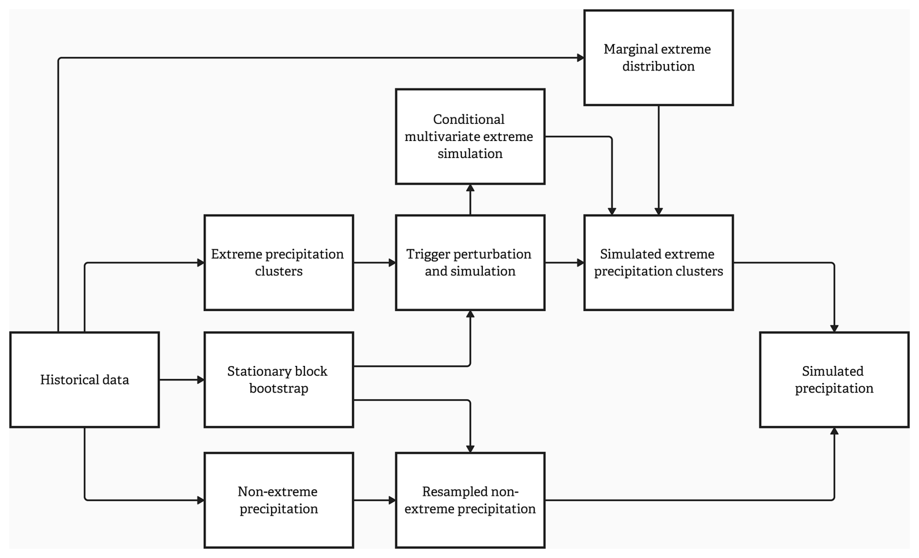
Figure 3 Schematic of the benchmark approach to weather generation. The method combines a stationary block bootstrap for non-extreme precipitation with a conditional multivariate extreme-value model for extremes. Extreme precipitation clusters are perturbed using historical dependence structures, then merged with resampled non-extreme precipitation to produce full synthetic precipitation fields.

The benchmark is a hybrid simulation technique that captures the underlying climatology via statistical bootstrapping and extremes via a conditional multivariate extremal dependence model (Fig. 3). The hybrid formulation has been used both for direct river flow estimation (Keef et al., 2013; Lamb et al., 2010; Quinn et al., 2019) and for precipitation modelling that is then used as input to hydrological simulation (Brocca et al., 2011). Here, we use its precipitation-generation configuration to provide a like-for-like comparison with the AI-generated weather data.

Beyond its role in representing appropriate extremal dependence structures, the benchmark also serves as an essential evaluative reference given the limitations of the historical record. The historical record contains only a small number of such spatially extensive storms, limiting its usefulness for evaluating generative models. For this reason, we include a benchmark that is already widely used in operational flood risk applications. Importantly, the benchmark does not simply resample historical storms: it perturbs the magnitude, spatial structure and peak location while preserving the historically observed dependence structure. This produces a long, diverse, and dependence-consistent set of synthetic storms that allows us to assess how closely an AI weather model of interest reproduces a validated distribution of spatially coherent extreme, beyond what can be judged from the limited historical record alone.

2.5.2 Generation of synthetic benchmark precipitation

Precipitation extremes were modelled by treating storms as spatiotemporal clusters and first considering the long-range dependency structure (the spatiotemporal model of clusters) and, conditional on this, the short-range dependency structure (the spatiotemporal evolution within the cluster). Precipitation at any location was regarded as extreme on any day that it exceeds the 99th percentile of the historical data at that location. Extreme instances were grouped into clusters by considering sequential runs of days and a spatial distance threshold (Davison and Smith, 1990).

Here, a single cluster was permitted to have a 1 d temporal break and a spatial separation of up to 350 km. Both thresholds were chosen based on a regional study of the tail dependence in historical precipitation; tail dependence was calculated for a range of temporal lags and distance thresholds and an elbow point across the region of study was determined at which the dependence decayed (Ledford and Tawn, 1996).

The long-range structure of precipitation is modelled as a spatiotemporal point process. The size of the spatiotemporal domain considered prohibits a parametric point process under the limited historical data record (Keef et al., 2013), and so a non-parametric stationary block bootstrap model was used (Politis and Romano, 1994). Stationary block bootstrapping resamples the historical data from a uniform multinomial model, retaining annual blocks. To capture both inter- and intra-year variability, the block length was varied, with length (in years) following a Poisson distribution. The resampled blocks at an annual scale are joined at the beginning of the month with the fewest precipitation clusters to minimise discontinuity (in this case, February). Our focus is on an ensemble of independent winter seasons, and we generated 1000 resampled blocks of 3-months, each of which can either be from a single coherent historical year or from a disjoint pair of historical years straddling January and February. The long-range structure of the simulated precipitation is thereby defined by the block-bootstrap, with the frequency and region of extreme clusters being that in the resampled data.

The short-range structure of precipitation was modelled using a perturbation scheme coupled with the conditional multivariate extremal dependence model (Heffernan and Tawn, 2004; Ledford and Tawn, 1996). The cluster trigger was defined as the location with the highest quantile of precipitation on the first day. New clusters were simulated by first perturbing the trigger location, simulating the precipitation at the trigger, and then conditionally simulating the precipitation at all remaining locations and times in the cluster. The perturbation follows a transition probability field defined by Ledford and Tawn (1996) which represents the conditional probability that a location becomes the trigger given that a trigger has been observed at another location. It has been shown to capture the influence of both distance and topography on precipitation dependence effectively (Keef et al., 2009, 2013). For each resampled extreme cluster, a new trigger is simulated according to this probability field, and an extreme quantile is simulated uniformly. The conditional multivariate extremal dependence model (Heffernan and Tawn, 2004) was used to simulate the quantiles of precipitation at all other locations and times in the resampled cluster, dependent on the perturbed trigger and with an extreme covariance structure defined by that of the historical cluster. Simulated quantiles of precipitation are converted to actual precipitation via marginal extreme value distributions fitted independently to historical data at each location, thereby preserving spatial variations in the precipitation climatology as the cluster severity is resampled.

3 Results

3.1 Precipitation generation results

We first evaluate the precipitation fields generated by the benchmark statistical model and by PrecipHENS against the historical reference data, applying the four criteria (G1–G4) introduced in Sect. 2.1. These criteria assess whether each method reproduces the observed precipitation climatology (G1), spatial and temporal coherence (G2), representation of extremes (G3), and methodological robustness (G4). The subsections below address these in turn.

3.1.1 Reproduction of present-day climatology

Figure 4 shows the spatial distribution of the mean daily precipitation on wet days (> 1 mm) and the number of wet days across the historical dataset, the benchmark simulated dataset, and PrecipHENS dataset. The two simulated datasets reproduce the major climatological features of winter precipitation across the Elbe region shown in the historical data, including increased precipitation in the south-west and lower totals in the north and central basin. The benchmark closely matches the observed spatial gradients and magnitudes, which is the result of the stationary block bootstrap on non-extreme precipitation. PrecipHENS also demonstrates strong agreement with the observed climatology, successfully capturing the large-scale spatial structure and key precipitation gradients across the region. The number of wet days is consistent across all datasets, indicating that both methods realistically simulate precipitation occurrence. A view of the bias between the historical dataset and both the benchmark and PrecipHENS is provided by Fig. B1. This shows a dry bias in PrecipHENS in the wettest regions of the domain. However, this bias is small and within 0.5 standard deviations of the historical record. These results demonstrate that both approaches (benchmark and PrecipHENS) preserve the key features of observed winter precipitation climatology (G1). PrecipHENS produces additional meteorological variables, including surface temperature as used for hydrological modelling. As such, Fig. B1 gives the equivalent of Figs. 4 and B2 gives the equivalent for surface temperature, demonstrating overall that PrecipHENS also preserves the historical winter surface temperature climatology.

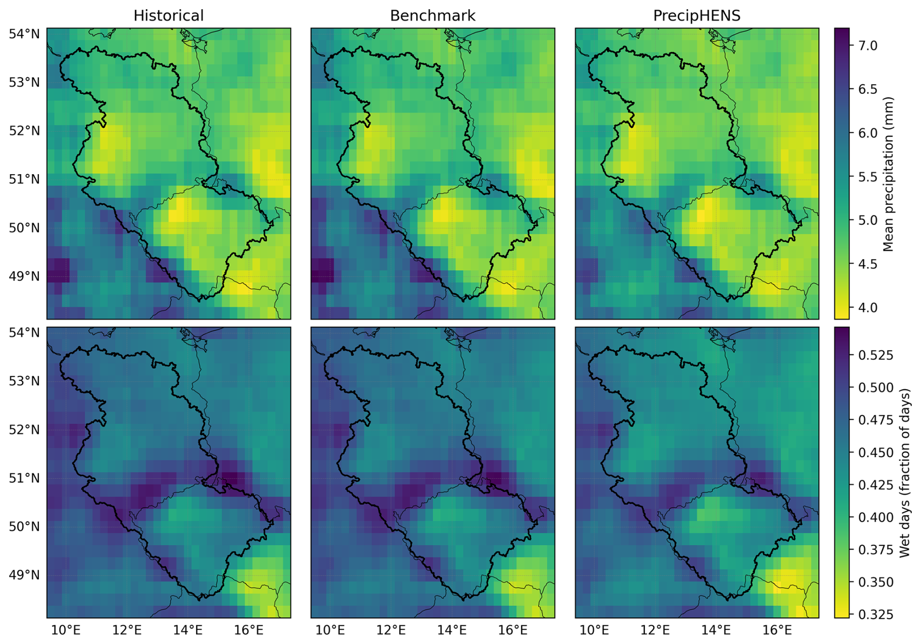
Figure 4 Comparison of mean daily precipitation over wet pixels (> 1 mm, top row) and the fraction of days with precipitation > 1 mm (bottom row). In each case data is presented from the historical (left), the benchmark (centre), and PrecipHENS (right).

3.1.2 Representation of spatial and temporal dependence

We assess spatial dependence in daily precipitation through two metrics: the Pearson correlation (r) (Pearson, 1895) and the Ledford–Tawn tail coefficient (η) (Ledford and Tawn, 1996). Pearson's r is a summary of the correlation in the bulk of the precipitation distribution, capturing the spatial organisation of typical precipitation variability. As flood risk is primarily driven by rare and spatially extensive extremes, the correlation specifically in the tails of the precipitation distribution is explored with η. This metric characterises the strength and decay of extremal co-occurrence between pairs of variables (locations, here).

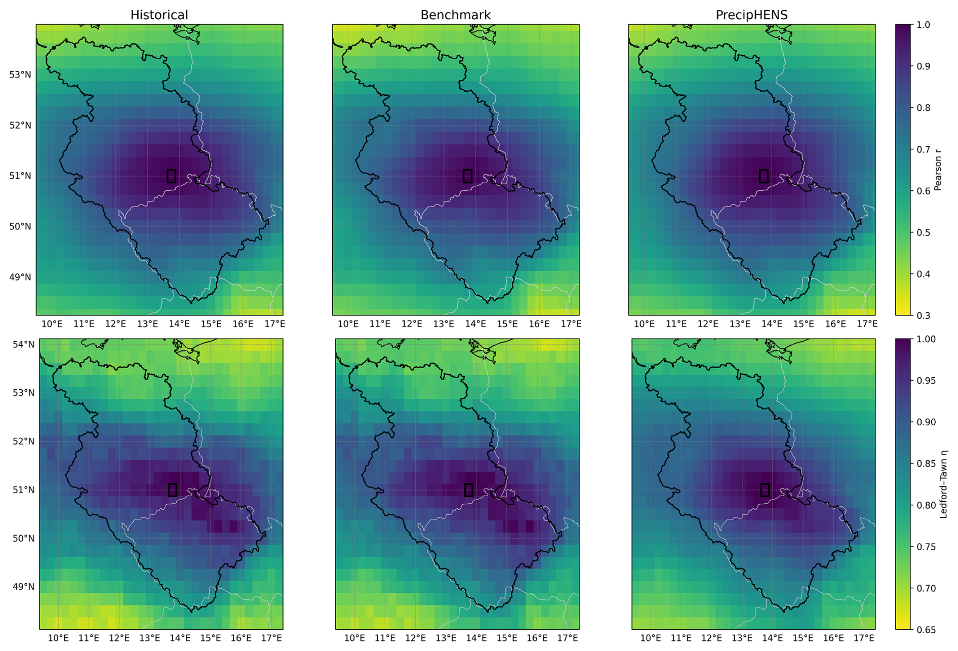
Figure 5 Correlation between daily precipitation at a reference location (Dresden; black square) and all other grid cells, computed across the winter period. Panels show results for historical data (left), benchmark simulations (centre), and PrecipHENS simulations (right). Correlation is shown for all data with Pearson's r (top row) and for extreme correlation with the Ledford–Tawn tail dependence coefficient (η) (bottom row, quantile threshold of 0.9).

Correlation fields of daily precipitation with a single location (Dresden) are shown in Fig. 5 and demonstrate that all three datasets – historical, benchmark, and PrecipHENS – exhibit similar spatial gradients and correlation decay. For the tail correlation, the results for η show that the benchmark approach reproduces the large-scale spatial structure of the historical data but also inherits its local variability, due to being constructed directly from a finite sample of past extreme events. In contrast, PrecipHENS yields a smoother spatial field that aligns with the dominant features seen in the historical data but avoids replicating its local sampling noise. Compared to the historical data, this smoother structure arises from the use of a much larger set of diverse, simulated seasons, allowing for more stable estimation of tail dependence patterns across space. In contrast, the typical precipitation correlation represented by Pearson's r has a smooth gradient across all three datasets owing to the larger sampling size, even in the historical record length.

For the tail correlation, Fig. 6 extends the single site results presented in Fig. 5 to evaluate whether this behaviour holds more generally across the domain, computing η from each location to all other grid points and grouping the results by distance.

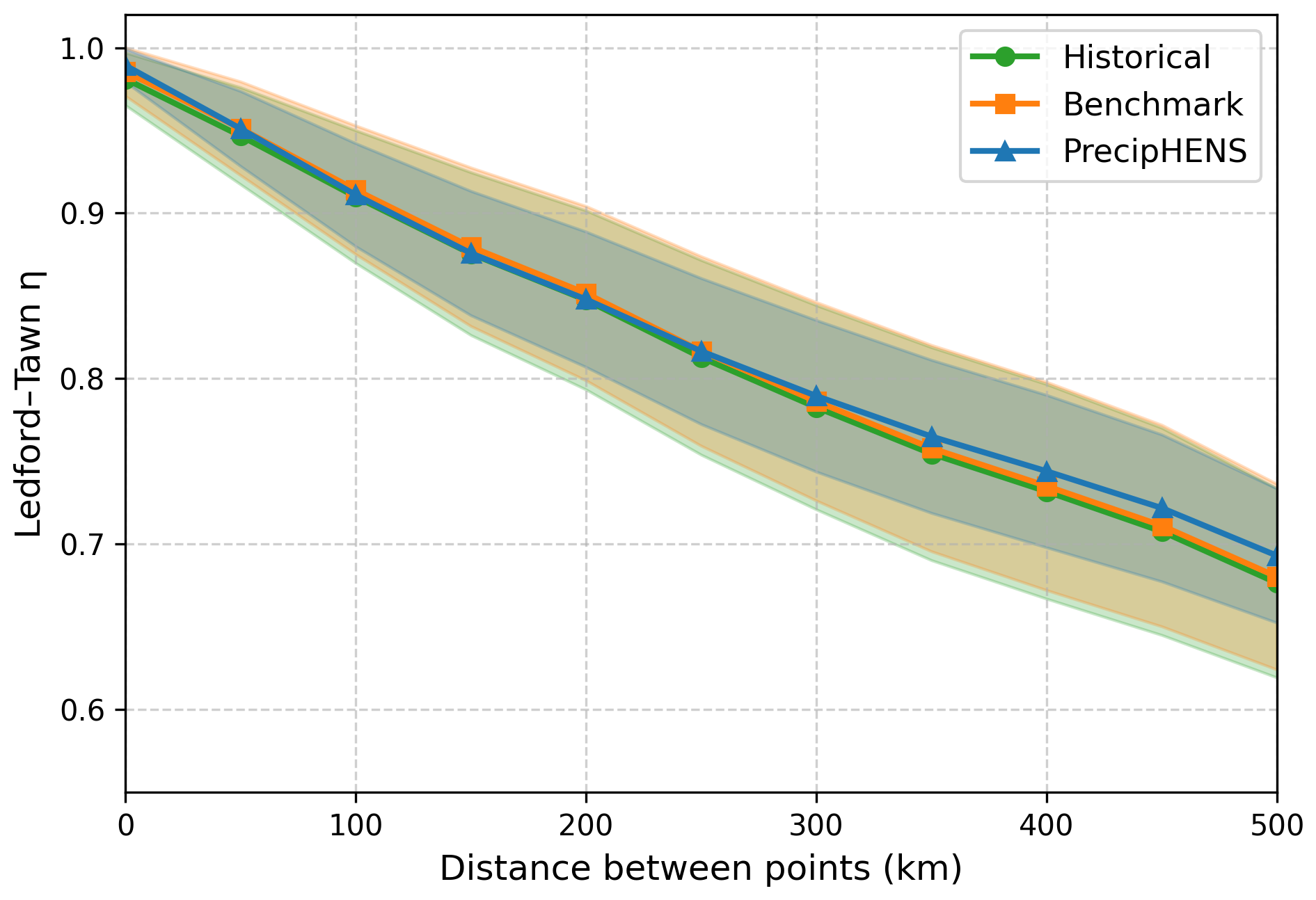
Figure 6 Ledford–Tawn tail dependence coefficient (η) as a function of distance between grid point pairs, computed from all grid points. Curves show historical data (green), the statistical benchmark (orange), and the PrecipHENS ensemble (blue), with shaded bands indicating ±1 standard deviation.

All three methods exhibit the expected monotonic decay in η with distance, reflecting the weakening spatial dependence of extremes at greater separations. The benchmark and PrecipHENS both closely follow the historical curve, confirming that it reproduces the same underlying extremal structure. The PrecipHENS ensemble displays a narrower uncertainty band compared to the historical and benchmark data, which may indicate the smoothing across events arising from its ability to sample a wide range of plausible events, particularly between locations of higher distances apart that feature fewer joint events in the historical record.

Temporal correlation in precipitation at a location is a key aspect for flood risk estimation because of the importance of compound or prolonged rainfall episodes in determining the ground saturation that impacts river flow. We assess temporal dependence in daily precipitation using the same two metrics as above – Pearson's r and η – each at a lag of 1 d. Pearson's r at lag-1 day provides a summary of linear dependence in the bulk of the precipitation distribution, reflecting how typical wet or dry days relate to conditions on the previous day; η complements this by characterising extremal persistence, measuring the likelihood that large precipitation values occur on consecutive days.

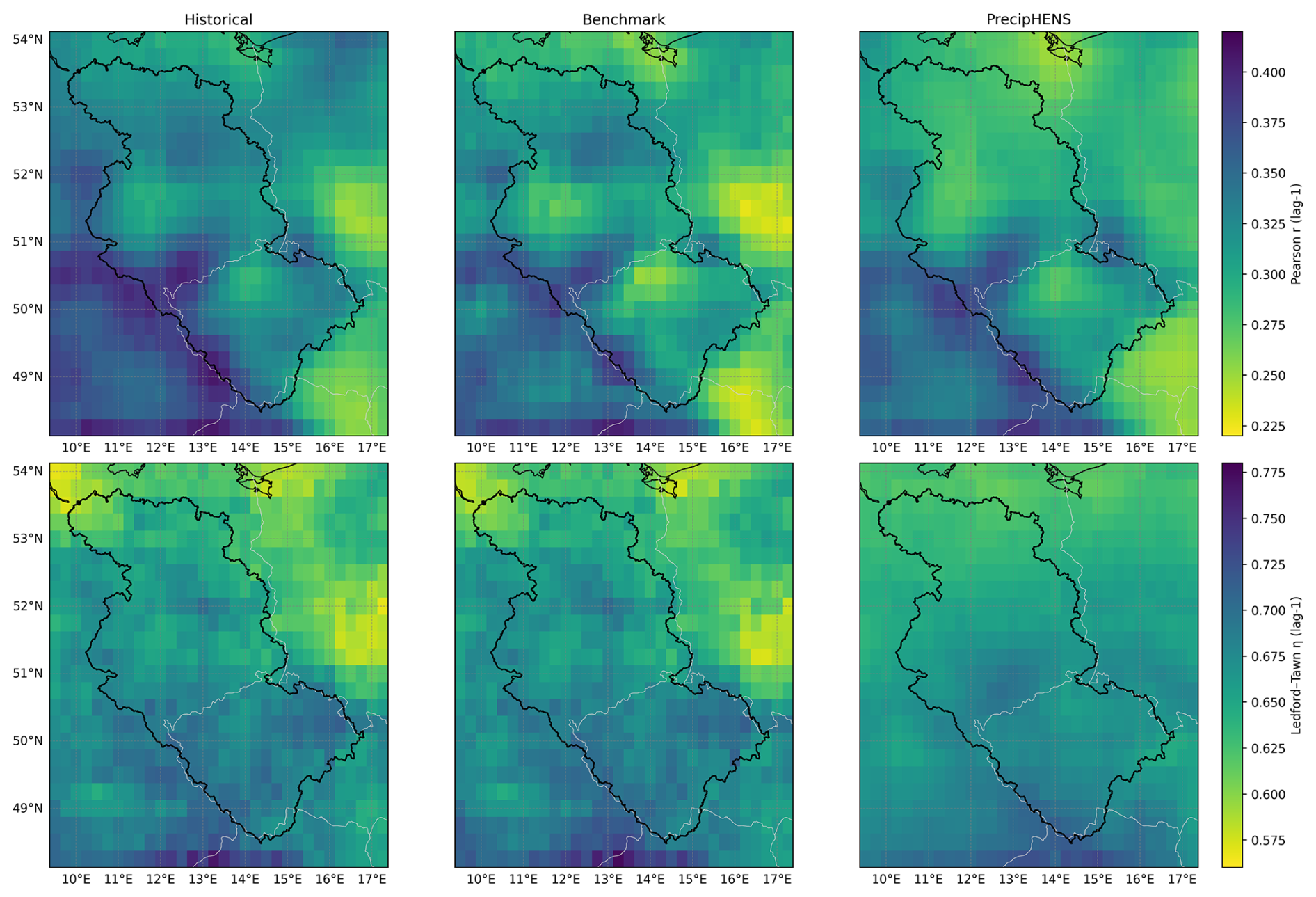
Figure 7 Correlation between daily precipitation at a location and the following day (i.e. 1 d lagged correlation per site), computed across the winter period. Panels show results for the historical data (left), benchmark (centre), and PrecipHENS (right). Correlation is shown for all data with Pearson's correlation (top row) and for extreme correlation with Ledford-Tawn tail dependence coefficient (bottom row, quantile threshold of 0.9).

Figure 7 shows maps of these temporal correlation metrics computed at each grid cell for the three datasets. The benchmark and PrecipHENS simulations again broadly reproduce the temporal structure seen in the historical record. PrecipHENS displays smoother spatial variation than the benchmark, but also lower similarity in general across the domain – again, likely a construct of the benchmark being constructed by resampling and perturbation from a finite sample of multi-day historical events. Additional evidence for this comes from inspecting the durations of wet spell events over the season at the example site of Dresden (Fig. B3) noting that the noise in the small sample of multi-day wet spells in the historical record drives what is seen in the benchmark data.

These results demonstrate that both approaches (benchmark and PrecipHENS) preserve the key features of observed spatial and temporal coherence, but that PrecipHENS is not sensitive to the limited observed tail variability in the historical record (G2). The spatial correlation in the temperature displays a smooth surface across all datasets, like the precipitation example in the top row of Fig. 5. We do not include this here for brevity, nor do we include tail temperature correlation because extreme temperature is not the focus of this present study.

3.1.3 Statistical tail behaviour of extreme events

Both the frequency and magnitude of precipitation extremes influence flood risk, so biases in either can distort risk estimations. Having already examined spatial correlation of extremes (e.g. in Fig. 5), we now assess the marginal behaviour of daily precipitation extremes at each grid cell. Rather than reproducing the historical record – which is too short for reliable tail estimation – we evaluate whether the simulations exhibit plausible distributions and spatial patterns in their extremes. The creation of long stochastic datasets such as the benchmark and PrecipHENS is motivated precisely by this need to explore physically realistic but unobserved extremes.

For each of the historical, benchmark, and PrecipHENS datasets, we compute the seasonal maxima of daily precipitation at each location and fit a Gumbel distribution via maximum likelihood. The Gumbel distribution – a special case of the generalised extreme value (GEV) distribution that fixes the shape parameter – is used here to avoid instability in fitting across locations. The GEV shape parameter can be highly uncertain for short historical records, leading to inconsistent tail behaviour across the region.

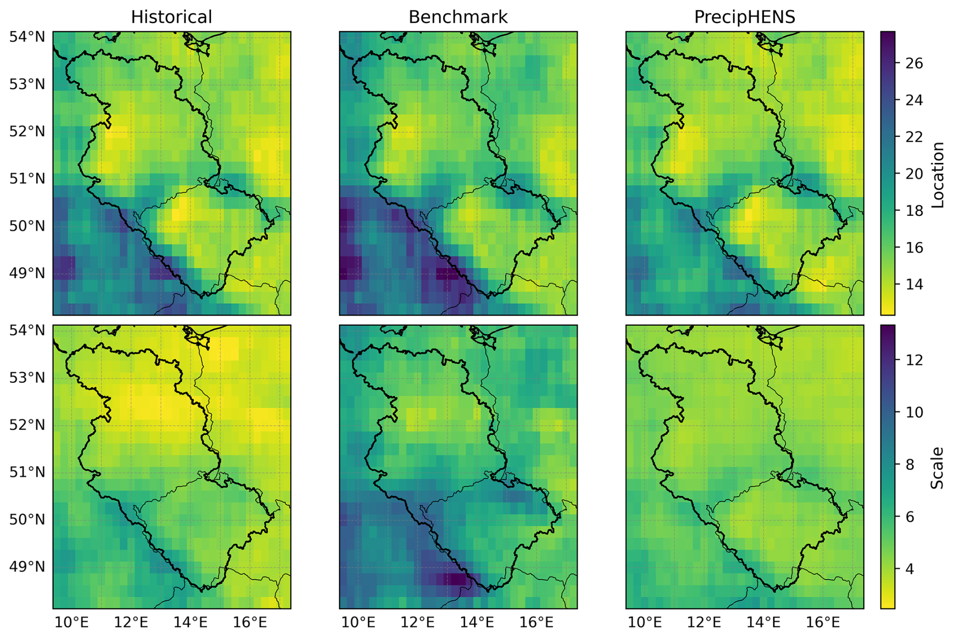
Figure 8 Extreme marginal distributional fit for 1 d precipitation, based on a Gumbel distribution fit to winter maxima. The location (top) and scale (bottom) parameters are shown for the historical period (left), benchmark (centre) and PrecipHENS (right).

The location and scale parameter fits are shown in Fig. 8 for each dataset. The spatial patterns in regions of higher Gumbel location parameter (thus higher precipitation extremes) and higher Gumbel scales (thus higher precipitation extreme variability) are similar. However, the benchmark model data displays higher fitted values of both Gumbel parameters than PrecipHENS. The local, marginal Gumbel parameters of the PrecipHENS simulations are closer to those of the historical data than are the benchmark model's, even though the benchmark model is based on inference about the extremes, whereas the PrecipHENS is a more general model. There is a generally coherent, smooth spatial structure in the tail distributional fits across the region, which, although fit independently per site, is consistent with the evidence of Fig. 5 that there is high spatial correlation in the extreme precipitation.

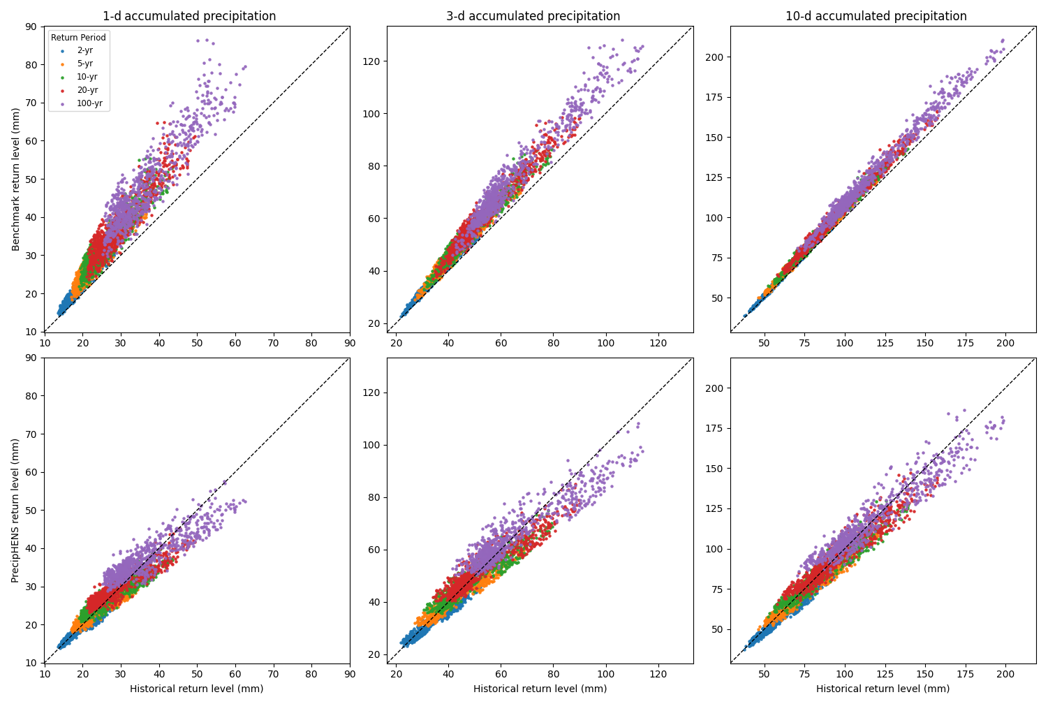
Figure 9 Comparison of modelled (benchmark in top row, PrecipHENS in bottom row) and historical precipitation return levels for a range of return periods (2, 5, 10, 20, 100 years) and durations (1, 3, 10 d). Each dot represents a single grid point. The different return periods are differentiated by the colours. The black 1 : 1 line indicates perfect agreement between modelled and historical return levels. Return levels are estimated using Gumbel fits to each respective dataset, for example in the case of the 1 d accumulated precipitation (left-most column), this is the Gumbel fit shown in Fig. 8.

To understand the joint contribution of the two parameters in the Gumbel fits, Fig. 9 gives the return level for precipitation for a range of return periods (2, 5, 10, 20, 100 years) at each site across the region, comparing this level under the model fitted to the historical data and the benchmark or PrecipHENS, respectively. A perfect agreement between historical and simulated fit is given by the dashed line for reference, and although it is not expected that (or an aim for) the data sit on this line, there is an expectation for a spread around the agreement line that increases with the return period and the associated uncertainty in estimation of such a return level with the limited historical data record. For example, the 2-year return level should be well estimated by the historical data (being 44 years in length) and we therefore expect there to be strong agreement between the simulated and historical data, whereas the 100-year return level is not well estimable from the historical data and is expected to have high spread. An example that highlights the uncertainty associated with the historical data under increasing return periods is shown in the appendix, Fig. B4, for the location at Dresden. In this example, the precipitation estimates associated with high return periods are higher in both the benchmark and PrecipHENS than the historical data (i.e. the Dresden grid cell would be one of the points above the reference line in Fig. 9), however the entirety of the PrecipHENS 95 % confidence interval sits within the associated historical interval.

In addition to the 1 d precipitation model results from Fig. 8, GEV models are fit to longer accumulations of 3 and 10 d, to explore the temporal structure of the extremes. Figure 9 suggests that the benchmark approach tends to over-represent the tail of precipitation, and that this over-representation accelerates as the tail becomes more extreme. This is likely due to the methodology of the statistical extrapolation, whereby the historical events are repeated and perturbed at the rate of the limited historical record, without consideration of whether the representation in the historical record is uniformly likely. For example, the method is sensitive to the presence of a rare, extreme event that is in the historical input record and is likely over-sampling the rarest, most extreme observed events. The return levels of PrecipHENS are more in agreement with the historical data at low return periods (2–10 years) than the benchmark method and are distributed around the agreement line at the higher return periods (20–100 years). Compared to the historical data, the variability from the historical distributional fits for the PrecipHENS data at high return periods tends to show that the return level is inflated for sites with lower extreme precipitation magnitudes and deflated for sites with higher extreme precipitation magnitudes.

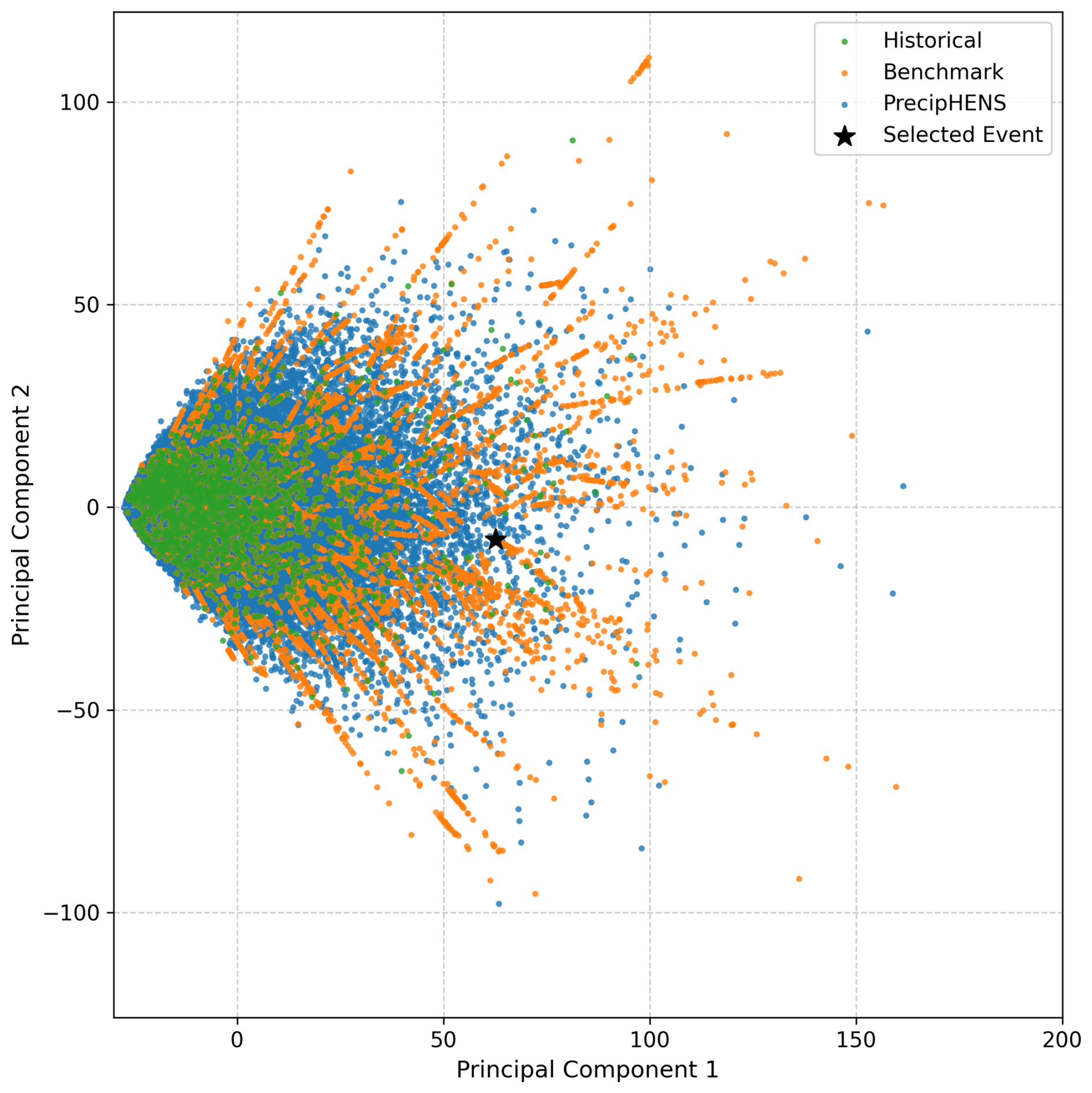
Figure 10 Principal component analysis (PCA) of daily extreme precipitation fields from the Historic, Benchmark, and PrecipHENS datasets. Each point represents a single extreme day projected onto the first two principal components (PC1 and PC2), summarising the dominant spatial variability in precipitation patterns. The starred point indicates the highlighted observed event (21 December 2023), shown in Fig. 11.

The marginal tail distribution results presented here suggest that the PrecipHENS data features extreme precipitation at an acceptable frequency and magnitude (G3): it is similar to the historical data and improves upon a likely over-sampling of repeated extremes in the benchmark approach, which occurs when it is built on a limited record of historical input data. This is a promising result for the AI-powered weather generation, which has previously been critiqued for a lack in ability to generate extremes (Mahesh et al., 2024), albeit the analysis here is conducted on aggregated values and not the 6-hourly temporal resolution the SFNO model outputs. The joint tail distribution across sites has been explored in the correlation discussion of the previous section, and we also explore the distribution of precipitation events as high-dimensional spatiotemporal clusters in the next section, showing that PrecipHENS has a smooth extrapolation from the historical examples of precipitation storm features (see Fig. 10).

3.1.4 Robustness and generalisability beyond the historical record

Statistical models for weather generation, such as the Heffernan and Tawn (2004) framework, are inherently tied to historical data since they construct multivariate relationships based on observations. While these approaches effectively capture statistical extremes within the historical record, they are fundamentally limited by the length and completeness of the observational dataset. As a result, they are constrained in their ability to produce new and unseen weather events. In contrast, AI models such as SFNO are designed to learn a latent representation of the underlying dynamics and interactions between meteorological variables. SFNO captures the spatial and temporal dependencies across the full atmospheric system, allowing it to generalise beyond the direct constraints of historical data (Bonev et al., 2023). Furthermore, SFNO-powered ensembles, such as the HENS approach have shown that these ensembles can produce plausible, yet novel extremes (Mahesh et al., 2024).

To compare the structural variability in extreme precipitation across the historical, benchmark, and PrecipHENS datasets, we perform a principal component analysis (PCA) on grid-point-level precipitation fields. The PCA is fitted to the historical data, for days which have a precipitation value exceeding the 90th percentile threshold for that grid point. This analysis provides insight into the dominant modes of variability in the historical extreme precipitation days, helping assess whether the different precipitation generation methods generate variable weather patterns and – because the PCA is fit only to historical data – how this extrapolation in the simulated data relates to the structure in the historical data.

Figure 10 compares the first two principal components (PC1 and PC2), with points coloured by dataset. These two components account for 67.8 % of the total variance in the historical extreme precipitation data (46.5 % and 21.3 % for PC1 and PC2, respectively), offering meaningful low-dimensional representation. Many of the benchmark points follow distinct vectors originating from near the origin. These vectors reflect the constrained modes of variability tied closely to the historical data used to construct the benchmark. The increased severity of extremes in the benchmark dataset (as shown in Sect. 3.1.3) is reflected with the points extending further from the origin than in the other two datasets. In contrast, PrecipHENS produces a more continuous spread of points, introducing a wider distribution of precipitation patterns whilst also extrapolating beyond the historical data.

To quantify how broadly each dataset captures this PCA space, we compute the proportion of non-overlapping 1 × 1 grid cells in PCA space that contain at least one event from each model. PrecipHENS spans 80.9 % of these cells, compared to 50.1 % for the benchmark and 18.8 % for the historical record. This reinforces the conclusion that PrecipHENS generates a broader diversity of extremes than the other methods. We note that this grid-cell count is intended only as an illustrative summary of the relative spread of events in the PCA projection. The PCA space does not represent the full set of plausible atmospheric extremes, and occupying a wider region of this space indicates greater structural diversity in the projected fields rather than a formal measure of physical plausibility.

The starred point in Fig. 10 marks an extreme day from the historical data drawn from outside the SFNO training period (21 December 2023). This event provides a representative out-of-sample precipitation pattern against which simulated extremes can be compared. Figure 11 shows the spatial precipitation pattern associated with the event. The event serves as a meaningful anchor in PCA space against which simulated extremes can be compared. To assess how each method reproduces physically plausible yet varied extremes, Fig. 12 shows the precipitation patterns for the eight nearest events in PCA space for the benchmark and PrecipHENS. All 16 events – i.e., eight events from both datasets – are close in PCA space, reflecting broadly similar storm structures across methods. However, clear differences emerge in the diversity of spatial precipitation patterns.

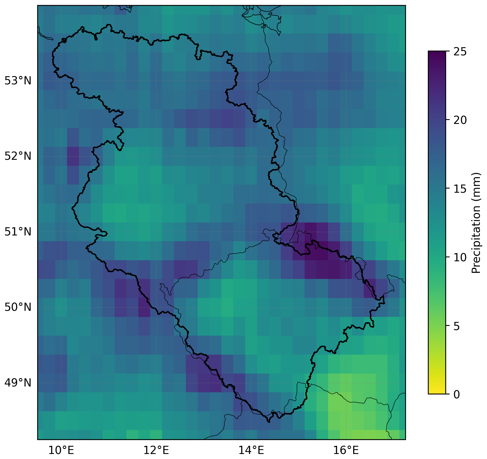
Figure 11 The precipitation pattern of the starred event in Fig. 10, representing the most extreme observed event impacting Dresden from the historical data, based on the maximum 1 d precipitation over the grid cell covering central Dresden.

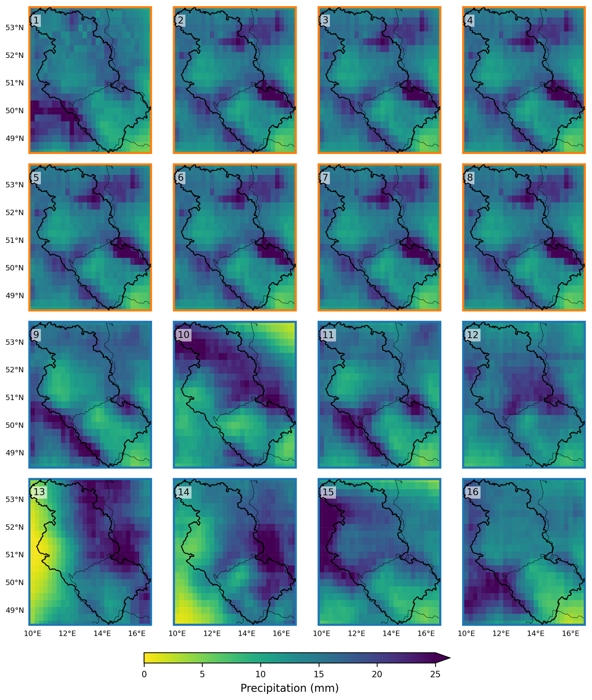
Figure 12 Precipitation fields corresponding to the eight simulated events that are closest in PCA space to the historical reference event, drawn, respectively, from the benchmark model (plots 1–8, top two rows with orange outline) and from PrecipHENS (plots 9–16, bottom two rows with blue outline).

The benchmark method events display limited variability, with similar spatial footprints and precipitation concentrated in nearly identical regions across panels for seven of the eight events, matching that of the historic event in Fig. 11. This repetition reflects the structural constraint of the statistical benchmark model, which, despite reproducing extreme values, tends to repeat historical spatial configurations with minimal deviation.

In contrast, the PrecipHENS events exhibit a broader range of spatial characteristics. While the overall structure of the storms remains similar (as expected given their PCA proximity to the historical reference), there is more noticeable variation in the location of precipitation maxima, the extent of wet areas, and the storm footprint shape. This highlights the SFNO model's ability to produce diverse and novel patterns, even when constrained to closely match a known historical extreme, supporting the model's potential to simulate a wider range of realistic high-impact events (G4).

3.2 Hydrological modelling results

This section describes the use of the simulated weather from the 1008-member winter seasonal ensemble of PrecipHENS as input to a hydrological model, along with initial catchment conditions from the modelled historical period. The four goals from Sect. 2.1 related to estimation of tail risk are revisited in relation to the simulated river flow as a dataset for flood risk estimation.

3.2.1 Reproduction of present-day climatology

Figure 13 shows the spatial distribution of mean river flow for large catchments (> 2500 km²) in the historical and PrecipHENS datasets, alongside the standardised bias between them. The historical climatology is calculated as the average of the 43 seasons of historical flow, whereas the PrecipHENS climatology is the average of 1000 bootstrapped samples, each of which is a sample of 43 seasonal simulations from the 1008-member ensemble combined with the historical sequence of initial catchment conditions. The bootstrap sampling design used here is to ensure a fair comparison of the bias in weather-driven flows as opposed to initial seasonal conditions, with each 43-member bootstrap sample from PrecipHENS including one ensemble member aligned with each of the 43 historical initial conditions. The PrecipHENS simulations closely reproduce the observed large-scale patterns in the historical data, with peak flows in the central and downstream regions and weaker flows in the south, east and west. The bias of PrecipHENS versus the historical data (Fig. 13, right) is small and consistently negative, falling within a modest range below one standard deviation of the historical data.

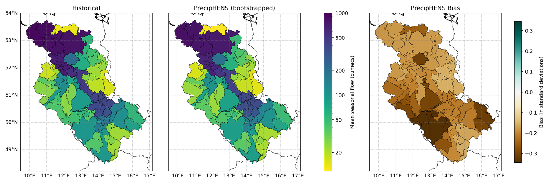
Figure 13 The average winter seasonal flow, shown only for catchments in the Elbe with area above 2500 km² (all catchments are shown in a version in Fig. C1). The historical (left) and PrecipHENS (middle) seasonal means are shown, along with the bias between these (PrecipHENS minus historical), standardised by the standard deviation in the historical seasonal mean (right).

Figure C1 shows the results highlighted in Fig. 13 but for all catchments across the Elbe basin. This confirms that the agreement between historical and PrecipHENS average flows extends across all catchments in the domain, not just the largest. The spatial structure and magnitude of mean river flows are consistently well reproduced, and the observed negative bias is modest and spatially coherent. While this points to a small dry tendency in the simulations, it is not large enough to affect the overall climatological fidelity and is not unexpected given that there was found to be a small dry tendency in the precipitation and a small warm tendency in the temperature (see Figs. B1 and B2, respectively). Together, these results confirm that PrecipHENS-driven simulations capture the key features of observed winter river flow climatology (G1).

3.2.2 Representation of spatial and temporal dependence

As in Sect. 3.1.2, we assess the spatial and temporal coherence of simulated river flows by comparing correlation patterns across the domain, using both Pearson's correlation coefficient (r) and the Ledford–Tawn tail dependence coefficient (η) to give a quantifiable measure of correlation across the basin in space and time. We also include an anecdotal example of river flow across the winter season and along the main trunk of the Elbe to illustrate the high temporal and spatial correlation that is generally present in river flow data (see Fig. C2 for a visualisation of this).

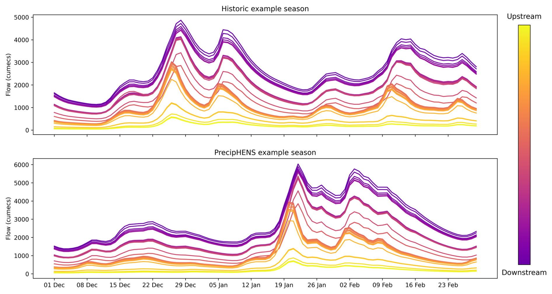
Figure 14 An example of hydrologically modelled river flow for an example historical season (top) and simulated PrecipHENS season (bottom) across the 30 catchments that form the main trunk of the river Elbe. See Fig. C2 for a map of this set of catchments.

Figure 14 shows time series of flow across the main Elbe trunk during a single example season from each of the historical and PrecipHENS datasets. It is important to note that these are two independent seasons, and so the goal here is not to compare them as like for like flow simulations that aim to match one another. From this example, the timing and progression of peaks clearly illustrate the propagation of flow through the river network, with PrecipHENS capturing upstream to downstream temporal evolution and magnitude increase in the flow.

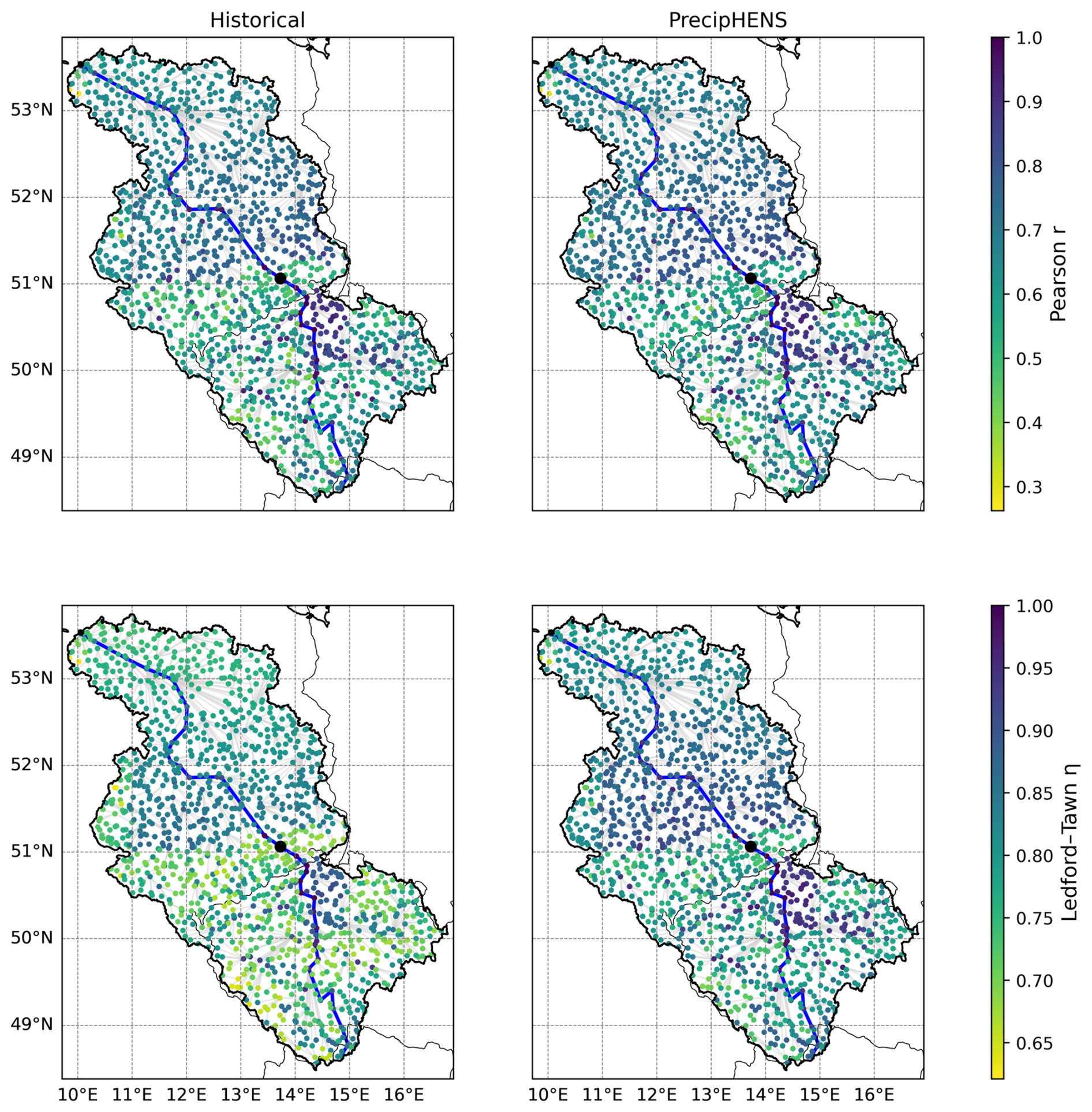
Figure 15 Correlation between daily river flow at a reference location (Dresden; black circle) and all other river catchments, computed across the winter period. In each case, only the outflow point of the catchment is shown as a point, and the grey connections highlight the structure of the river network, with the main trunk of the Elbe highlighted in the blue line. Panels show results for historical data (left) and PrecipHENS simulations (right). Correlation is shown for all data with Pearson's r (top row) and for extreme correlation with the Ledford–Tawn tail dependence coefficient (η) (bottom row, quantile threshold of 0.9).

Figure 15 shows spatial correlation patterns for the Dresden reference catchment, comparing PrecipHENS against the historical data. PrecipHENS captures the dominant spatial structure of flow seen in the historical record, including strong upstream-downstream coherence along the Elbe and weaker correlations across sub-basins. Unlike the precipitation correlation, which is expected to be a relatively smooth spatial field, the expected correlation in river flow between catchments will largely rely on three factors: the upstream-downstream network structure; the proximity between catchments, which influences their shared exposure to weather patterns; and the relative size of the contributing areas, with large upstream catchments exerting a stronger influence on downstream flow than smaller ones. This final point is illustrated in Fig. 15: several catchments south-east of Dresden show stronger correlations with the Dresden site, consistent with their higher average flows, as shown in Fig. 13.

While Pearson's r fields are closely matched in Fig. 15, the extremal correlations in PrecipHENS, represented by η, are generally higher than in the historical data, indicating modestly stronger extremal dependence. These differences likely reflect the larger ensemble size and richer sampling of extremes in PrecipHENS, which yields smoother and more stable estimates of extremal dependence compared with the more variable historical data, rather than any systematic bias. This behaviour is consistent with the precipitation results, where the noisy spatial pattern of η in the historical data is comparably smoother in the larger PrecipHENS ensemble.

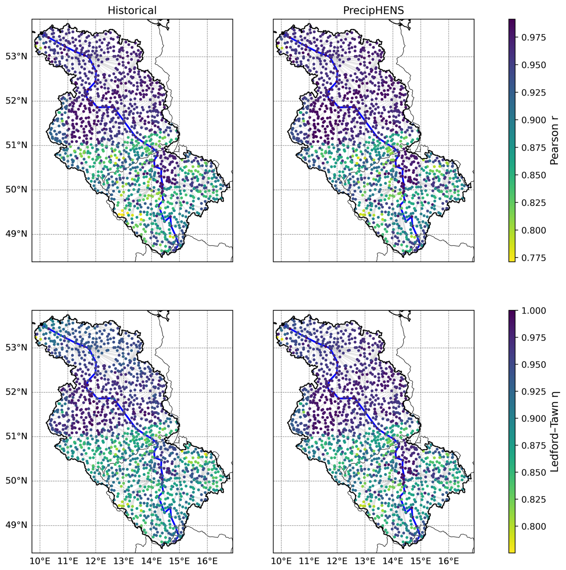
Figure 16 Correlation between daily river flow at each catchment and the flow at that respective catchment the following day (i.e. lag of 1 d), computed across the winter period. In each case, only the outflow point of the catchment is shown as a point, and the grey connections highlight the structure of the river network, with the main trunk of the Elbe highlighted in the blue line. Panels show results for historical data (left) and PrecipHENS simulations (right). Correlation is shown for all data with Pearson's r (top row) and for extreme correlation with the Ledford–Tawn tail dependence coefficient (η) (bottom row, quantile threshold of 0.9).

This temporal correlation at a single day lag is given in Fig. 16 (and at a 10 d lag in Fig. C3). The 1 and 10 d lagged Pearson's r and η values across the basin are comparable between PrecipHENS and the historical data. At a 1 d lag, the correlation – generally and in the extremes – is high across the region (lowest Pearson's r being above 0.7). This is particularly so in the northern region of the Elbe, explaining the clear separation between slow-responding catchments in the lowlands and fast-responding catchments in the more mountainous southern region. This demonstrates that PrecipHENS precipitation, when fed through the GR4J hydrological models, induces the strong autocorrelation expected in streamflow even without explicit river flow routing between the modelled catchments.

The anecdotal and quantitative examples presented here suggest that PrecipHENS preserves the spatial and temporal coherence of observed river flows across the Elbe network in comparison to the historical modelled data (G2).

3.2.3 Statistical tail behaviour of extreme events

Given the strong dependence of river flow extremes on precipitation input, and the established realism of precipitation extremes in Sect. 3.1.2, we expect PrecipHENS to also produce plausible hydrological extremes – provided the temporal sequencing of rainfall is well represented. As shown in Sect. 3.2.2, the temporal structure of precipitation and resulting flow is preserved, supporting this assumption.

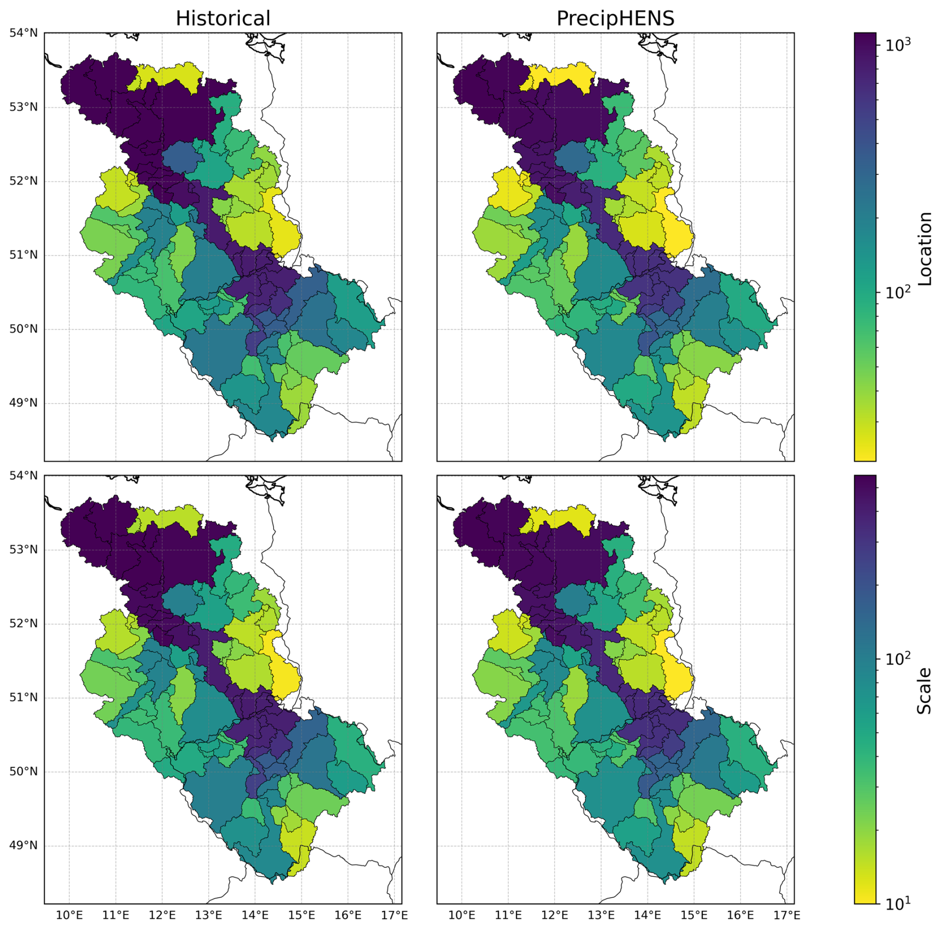
Figure 17 Extreme marginal distributional fit for daily river flow (in cumecs), based on a Gumbel distribution fit to winter maxima. The location (top) and scale (bottom) parameters are shown for the historical (left) and PrecipHENS (right).

To assess the marginal behaviour of flow extremes directly, we compute Gumbel fits to the seasonal maxima of daily streamflow at each catchment and compare the resulting location and scale parameters between the historical and PrecipHENS datasets. Figure 17 shows strong agreement in both parameters across the larger catchments, with PrecipHENS replicating the spatial structure of flow extremes seen in the historical record. These results support the conclusion that PrecipHENS produces realistic hydrological extremes across the basin (G3).

3.2.4 Robustness and generalisability beyond the historical record

Section 3.1.4 demonstrated that PrecipHENS produces a wide range of plausible yet structurally diverse extreme precipitation events, extending beyond the variability present in the historical or benchmark datasets. Figure 10 showed that PrecipHENS explores a broader region of the PCA space of extreme precipitation patterns, and Fig. 12 illustrated that these extremes differ meaningfully in spatial footprint and intensity, even when constrained to be close to a known historical event. Here, we evaluate the hydrological impact of these novel events.

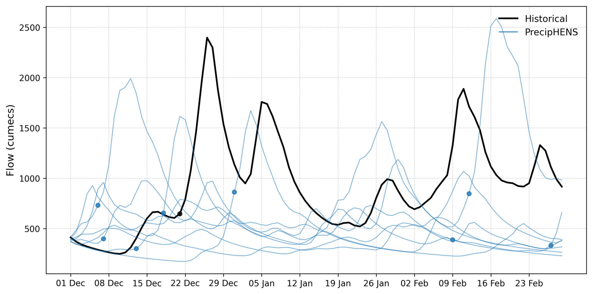
Figure 18 River flow at the Dresden reference location resulting from the eight PrecipHENS ensemble members closest in PCA space to the most extreme observed precipitation event (21 December 2023). Each line shows one season of flow simulation, driven by a distinct AI-generated precipitation pattern, with the blue point representing the time of the selected event. The black line shows the corresponding historical season.

Figure 18 shows the river flow simulations at Dresden resulting from the eight nearest PrecipHENS events (in PCA space) relative to the historic 21 December 2023 storm. Each of these simulations is driven by a precipitation pattern that is distinct from the observed event but similar in overall structure (as shown in Fig. 18). The resulting flow responses from each of the storms demonstrate the hydrological variability that PrecipHENS can produce from similar looking events.

To contextualise these results, Fig. C4 compares the full range of river flows simulated from the 43 historical precipitation seasons to the 1008 PrecipHENS simulations driven by a variety of initial catchment states. This wider ensemble view highlights the increased variability introduced by PrecipHENS. The frequency, severity, and timing of flow peaks differ noticeably from the historical record, offering a more diverse and expansive representation of extreme river flow risk. These results show that the methodological robustness and generalisability of PrecipHENS extend beyond atmospheric realism to hydrological impacts (G4).

4 Discussion and conclusion

This study introduces PrecipHENS, an AI-powered weather model designed to generate seasonal-scale synthetic weather ensembles for use in flood risk assessment and related extremes analysis. PrecipHENS combines the huge ensembles (HENS) framework based on the Spherical Fourier Neural Operator (SFNO) with the Precipitation AFNO diagnostic precipitation prediction model (Bonev et al., 2023; Mahesh et al., 2025; Pathak et al., 2022). By evaluating PrecipHENS against an established statistical benchmark – based on the conditional multivariate extreme-value model of Heffernan and Tawn (2004) – we demonstrate that AI-based weather generation provides a viable alternative for applications such as flood risk assessment and catastrophe modelling at 0.25° resolution.

PrecipHENS meets our four goals outlined in Sect. 2.1: reproducing observed climatology (G1), credible space–time coherence (G2), and credible extreme behaviour (G3) while maintaining methodological robustness (G4). Unlike traditional statistical models that perturb and extrapolate the historical record, PrecipHENS can generate new, physically consistent weather events that extend beyond observations – an essential capability for representing low-likelihood, high-impact events. When aggregated to the catchment scale, the resulting precipitation and temperature fields drive hydrological simulations that yield realistic river flow responses, confirming the model's suitability for flood risk assessment. Other frameworks also pursue this goal, such as the UNSEEN (Unprecedented Simulated Extremes using ENsembles) approach (Thompson et al., 2017; Kay et al., 2024), which pools large dynamical forecast ensembles to expand the plausible space of extremes. Unlike UNSEEN, which relies on computationally intensive physical forecast models, PrecipHENS achieves a similar outcome through efficient AI-based emulation, offering a flexible and cost-effective alternative.

Despite these strengths, several areas warrant further development. The hydrological modelling in this study assumed initial river conditions derived from an equal resampling of the 44 years of historical input data. A more sophisticated initialisation that captures the full range of seasonal variability and antecedent hydrological states could enhance the realism and variability of simulated flows. Scaling PrecipHENS to continental domains and extending simulations to year-round conditions would broaden its utility, particularly for catastrophe modelling where understanding risk across years and for continental-scale portfolios is essential. A broader and more diverse set of initial atmospheric states would likely increase ensemble variability and is a natural direction for future scaling of the framework.

An additional uncertainty concerns the physical plausibility of the meteorological fields generated by the underlying SFNO emulator, which, unlike physics-based dynamical models, are not generated by explicitly solving the governing equations of atmospheric motion. While our statistical evaluations demonstrate that PrecipHENS reproduces observed climatology and extreme-value behaviour, ensuring physical realism in long AI-generated sequences remains an open research challenge. Related to this, PrecipHENS inherits the implicit assumption of stationarity from its training data. While this is appropriate for representing present-day and near-term variability, it means the specific AI weather model used here – trained on ERA5 for 1979–2015 – will increasingly reflect the climate of that historical period if applied to far-future conditions, as the statistical properties of extreme precipitation evolve under ongoing climate change. We emphasise that this limitation applies to the current model instance, not to the PrecipHENS framework itself, which is model-agnostic and could in principle be paired with alternative training datasets for non-stationarity approaches in future work. We also note that assessment of future climate risk is not the goal of this study or within the use case of the benchmark model. Remaining uncertainties also concern how well SFNO reproduces large-scale atmospheric circulation patterns and teleconnections such as the North Atlantic Oscillation (NAO) and El Niño-Southern Oscillation (ENSO), which influence seasonal precipitation patterns. Climatological diagnostics also suggest some under sampling of longer-term variability (Fig. 4), indicating a need for further evaluation of how historical variability is represented in PrecipHENS.

The limited duration of the historical record also influences both the benchmark and PrecipHENS in distinct ways. The benchmark model inherits its dependence structure directly from the observed extremes, meaning its ability to represent rare spatial storm patterns is constrained by the limited variety present in the input record. In contrast, PrecipHENS learns dynamical operators from the ERA5 training period, enabling it to generate a wider range of spatially distinct extremes (as reflected in the PCA analysis), while still being conditioned on the same underlying historical climate state. Both approaches therefore extrapolate beyond the observational period, but the nature of this extrapolation differs between the statistical and AI-based methods.

While GR4J effectively captures the rainfall-runoff transformation at the sub-basin scale, the lack of explicit channel routing means that the temporal translation and attenuation of flood waves are not specifically modelled. The fluvial simulations are therefore physically independent between sub-basins and do not capture downstream interactions or continuity along the river network. The framework is designed to characterise the hydrological response to meteorological forcing and to reproduce the observed temporal and spatial correlation of flood events across locations, rather than to simulated routed hydrographs. Consequently, the conclusions of this study are most applicable to understanding how meteorological variability translates into coherent sub-basin flood responses, and less applicable in settings where flood-wave routing, floodplain storage, or prolonged multi-peak events dominate flood behaviour.

Integrating AI-powered weather generation into flood risk assessment has important implications for both research and practice. The ability of PrecipHENS to produce realistic, long-lead seasonal sequences enables generation of stochastic event sets that include plausible yet previously unobserved extremes. This opens opportunities to couple AI-generated meteorology with seasonal forecasts or storyline approaches (Shepherd et al., 2018), providing novel event sequences for stress testing and adaptation planning. The study outlines a practical framework for embedding AI weather emulators into the risk estimation workflows, showing that while AI models need not be developed in-house, effective use will depend on establishing interfaces between model developers and end users. Such collaboration will help tailor outputs for specific hydrological and risk applications and ensure that AI-driven weather generators evolve in ways that meet sectoral needs.

This work represents an initial but significant step toward integrating AI-powered weather simulations into flood risk estimation and catastrophe modelling. Demonstrating the feasibility of PrecipHENS for seasonal-scale weather ensembles and hydrological modelling provides a foundation for extending AI methods to larger domains and longer timescales. As AI weather models continue to advance, their inclusion in probabilistic risk frameworks will become increasingly valuable, offering new opportunities to characterise and manage flood risk in a changing climate.

Finally, we note that expert meteorological assessment of AI-generated weather remains limited for long rollouts of emulators like SFNO. These models are typically trained and validated for short-range forecasts. As AI weather generators become more widely applied in natural hazard risk analysis, collaboration with academic groups specialising in synoptic meteorology will be essential to evaluate physical consistency and diagnose potential systematic artefacts. The precipitation biases we observe in this study further underline the importance of understanding the mechanisms that produce such behaviour. We view this as an important direction for the community and one that will help ensure future AI-driven weather generators deliver both statistical and physical credibility.

Appendix A: Data sources for river catchment attributes

The dataset of 68 gauged and 1294 ungauged catchments (shown in Fig. 2) within the Elbe River basin modelled within this analysis were associated with a range of attributes to facilitate the modelling of the ungauged basins. This information was extracted from several global-scale datasets as described in Table A1.

Table A1 Catchment attribute data source.

Appendix B: Additional precipitation results

To extend the precipitation climatology in Fig. 4, a bootstrapped sample was performed with each sample being of the same length as the historical record (44 years) and taking 1000 bootstrapped samples. The bootstrapped mean is shown in Fig. B1, along with the deviation from the historical climatology. PrecipHENS shows a drier climatology than the historical data, but the difference is within 0.5 standard deviations of the historical mean, indicating that it lies well within the range of typical interannual variability rather than representing a significant bias. PrecipHENS also provides temperature in addition to precipitation, and so a view of the temperature climatology is shown in Fig. B2 in comparison with the historical data. As above, a bootstrapped sample was taken to compare. The bias shows a warmer climatology compared to the historical but is again within 0.5 standard deviations from the historical record.

Correlation in time is further explored to the 1 d lagged example in Fig. 7 by exploring in more detail the correlation at a single site. Figure B3 gives the distribution of wet day durations at the Dresden example site (where a wet day is defined as a day with > 1 mm precipitation). In Fig. 7 the correlation is highlighted as being generally lower in PrecipHENS than the benchmark and historical data, and Fig. B3 demonstrates that this is due to a higher proportion of single wet day events in the PrecipHENS data in comparison with the historical and benchmark data. In contrast there is a discontinuity in the historical and benchmark data at wet spell durations of 5 d, indicating again that noise in the short historical record drives the benchmark results.

Figure B4 provides a single-location return-level diagnostic (Dresden) to complement the basin-wide comparison in Fig. 9. Return levels are obtained from a Gumbel fit to winter block maxima with uncertainty bands estimated via a parametric bootstrap (refit on simulated maxima and take percentile intervals).

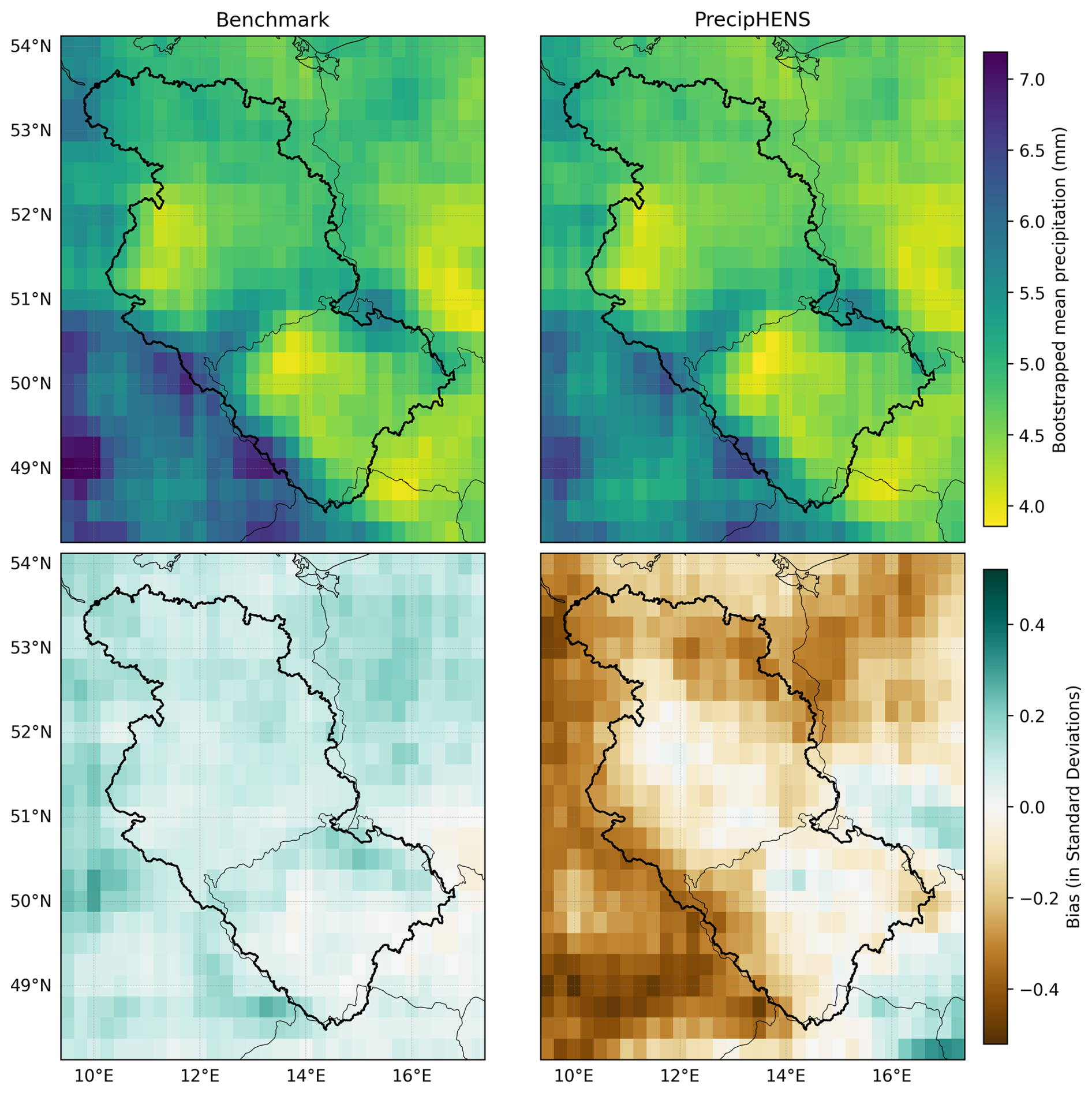
Figure B1 Comparison of mean daily precipitation over wet pixels (> 1 mm) as a bootstrapped sample (each sample being of the same length as the historical record (44 years) and taking 1000 bootstrapped samples, top row) and the bias compared to the historical climatology (bottom row). Data is presented from the benchmark (left) and PrecipHENS (right).

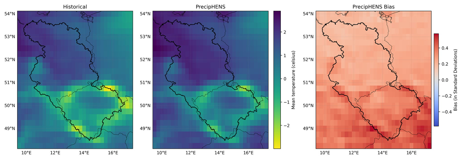
Figure B2 Comparison of mean daily surface temperature in the historical (left) and PrecipHENS (centre). The PrecipHENS data is presented here as the mean of a bootstrapped sample, and the bias from the historical is also shown (right).

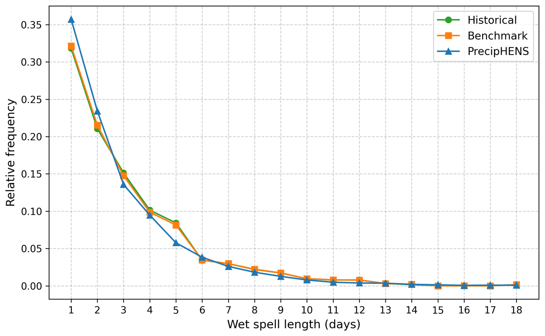
Figure B3 The proportion of multi-day precipitation across the historical, benchmark and PrecipHENS data for the Dresden location. A wet spell is defined as that with more than 1 mm daily precipitation, and wet spell duration is calculated as the number of consecutive days above this threshold. The data here is presented as the relative frequency of wet spell durations across those identified at the location.

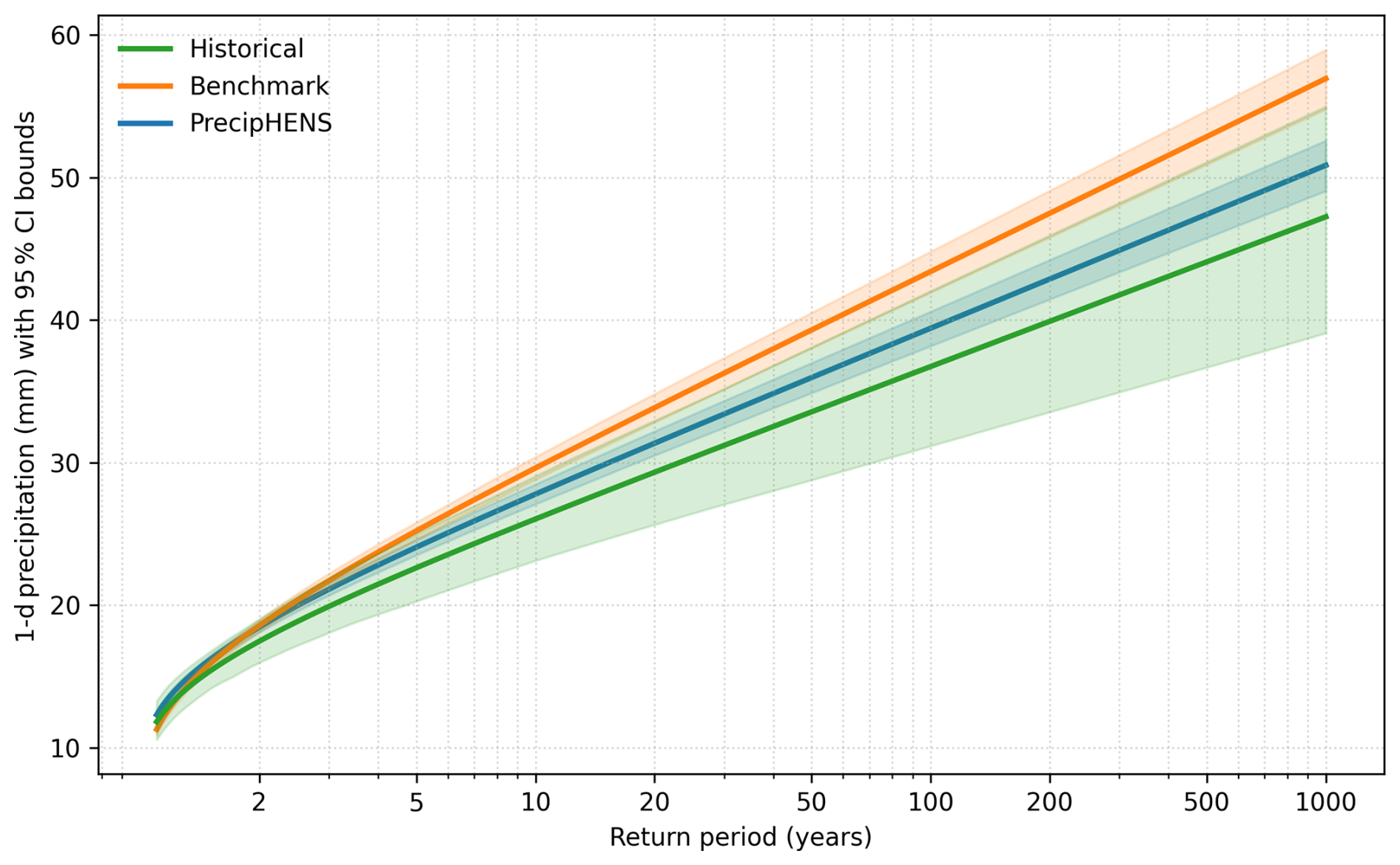
Figure B4 The estimated return period curve (with associated 95 % confidence interval) obtained by a Gumbel distributional fit across the historical, benchmark and PrecipHENS data for the Dresden location.

Appendix C: Additional hydrological modelling results

Additional examples of river results are included to support those presented in Sect. 3.2. The climatological river flow across the basin is extended to all catchments in Fig. C1 to support the version focusing only on large catchments in Fig. 13. This shows that in addition to the average flow being well represented in PrecipHENS at large catchments, this is the case across the basin. The temporal correlation in Fig. 16 is given at a lag of 1 d, and so Fig. C3 provides a longer-term correlation example at a lag of 10 d. Again, the coherent patterns and structure across the basin are recovered in PrecipHENS for both the average and the extremes.

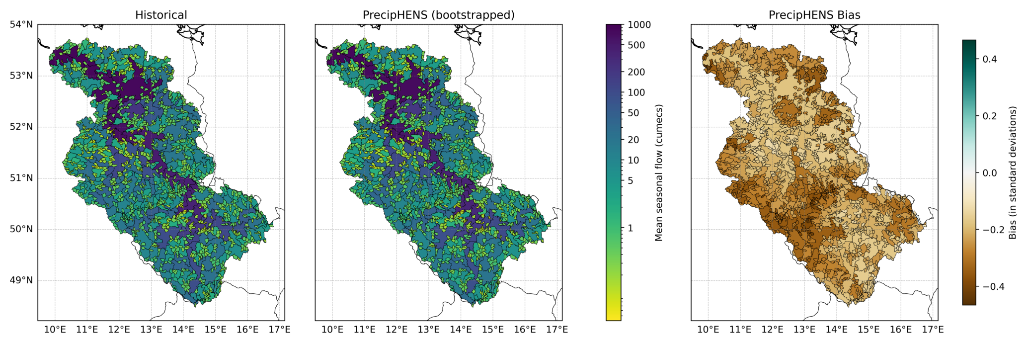
Figure C1 Mean seasonal river flow (in cumecs) for all catchments across the Elbe. See Fig. 13 for caption details, which shows a subset of larger catchments.

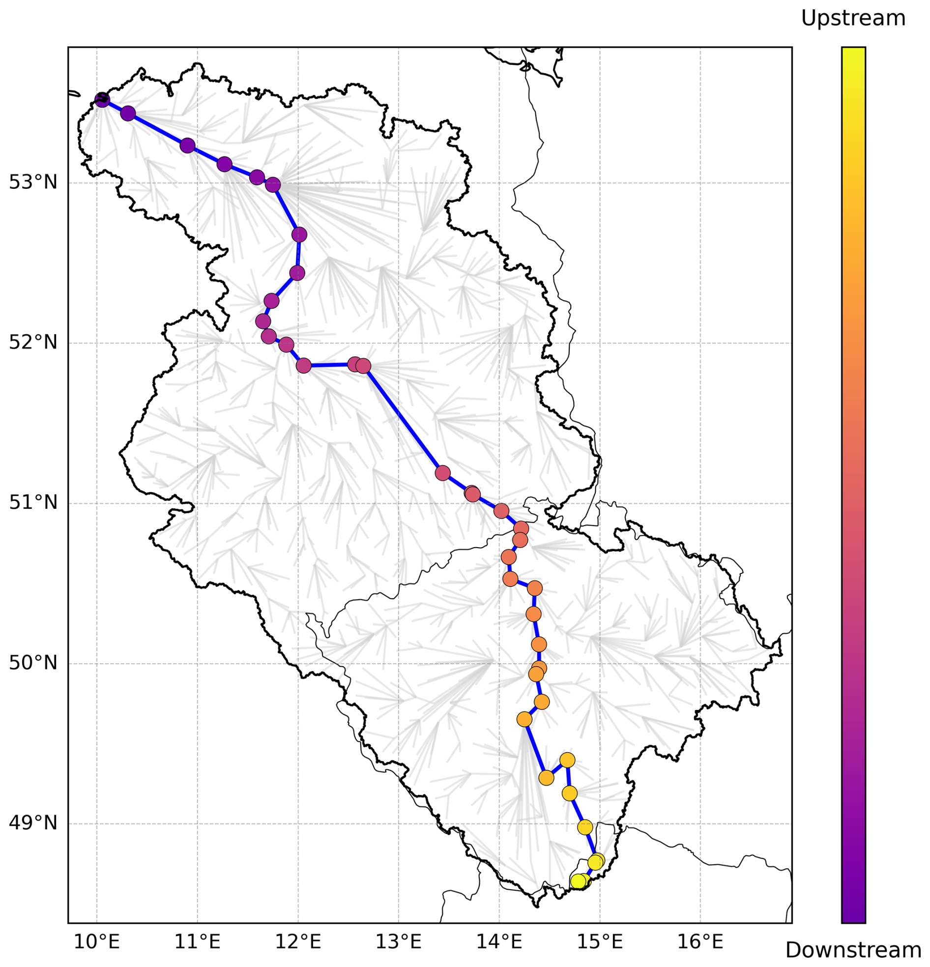
Figure C2 The catchments along the main trunk of the river Elbe, used in examples of Sect. 3.2. The Elbe basin is highlighted with the grey lines showing the network connections between catchment outflow points across the basin. The outflow point of the catchments along the main trunk are shown with the points, coloured by the upstream-downstream positioning (this colour scale is used in relevant figures such as Fig. 14).

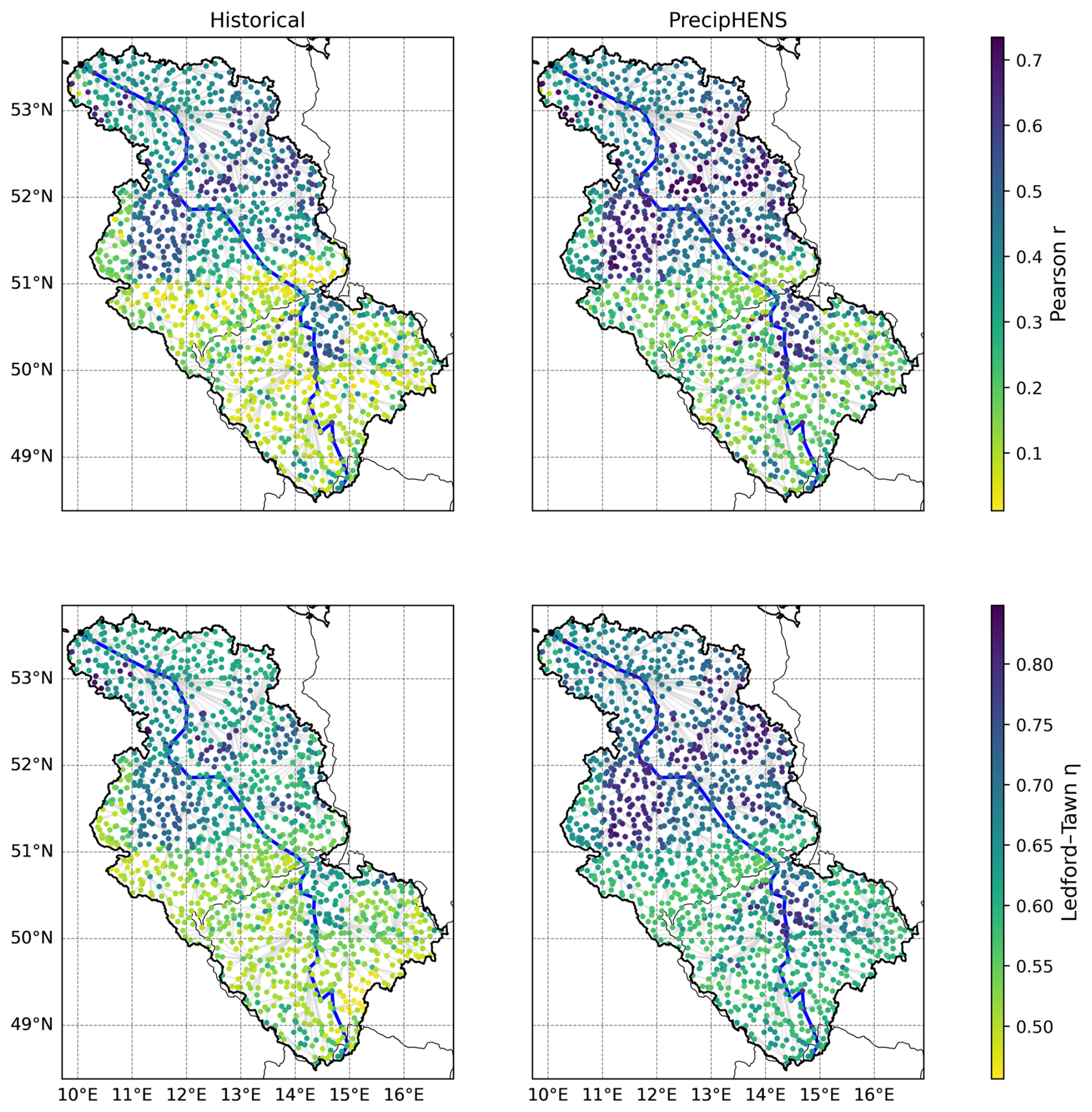
Figure C3 Correlation between daily river flow at each catchment and the flow at that respective catchment 10 d later (i.e., lag of 10 d), computed across the winter period. In each case, only the outflow point of the catchment is shown as a point, and the grey connections highlight the structure of the river network, with the main trunk of the Elbe highlighted in the blue line. Panels show results for historical data (left) and PrecipHENS simulations (right). Correlation is shown for all data with Pearson's r (top row) and for extreme correlation with Ledford–Tawn tail dependence coefficient (η) (bottom row, quantile threshold of 0.9).

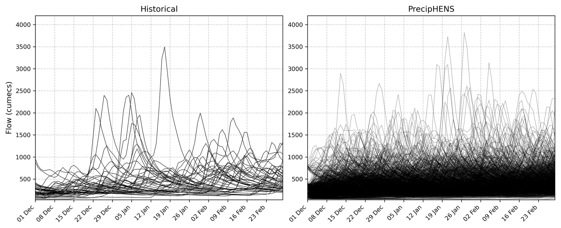
Figure C4 Full-season river flow simulations at the Dresden reference location. The historical data (left) are the modelled flows from all 43 historical precipitation seasons with their respective initial catchment conditions, while the PrecipHENS data (right) are each of the 1008 weather simulations paired with a random initial catchment condition (for visual clarity as opposed to all 43 344 flow simulations).