An improved empirical model for predicting postfire debris-flow volume in the western United States

Reliable estimates of debris-flow volume can be used to help predict the magnitude of debris-flow hazards following wildfire in the western United States. In this study, we compiled and used a database of 227 postfire debris-flow volumes that were collected across the western United States to develop a multiple linear regression model for predicting postfire debris-flow volume. We explored 36 predictor variables related to rainfall, terrain, and fire characteristics, and selected the model with the combination of variables that yielded the most accurate predictions of debris-flow volume. We evaluated model performance against the entire volume database, as well as against four subsets of volume data from southern California, the Intermountain West, the Southwest, and regions with limited volume data, such as northern California and Washington. We also compared model performance against 3 existing postfire debris-flow volume models that were developed for use in southern California, the Intermountain West, and the Southwest. We demonstrate that the new volume model performs as well as the regional models in the regions for which they were developed and outperforms existing models when applied to volumes from data-limited regions in the western United States. These results indicate that the debris-flow volume model introduced in this study can be used to improve postfire hazard assessments across the western United States, especially outside of southern California.

1 Introduction

Debris flows are a common hazard in mountainous areas around the world (e.g., Rickenmann and Zimmermann, 1993; Wang et al., 2003; Cannon and Gartner, 2005; Sepúlveda et al., 2006; Guthrie et al., 2012; Gartner et al., 2024) but are particularly prevalent in steep landscapes that have been recently burned by wildfire. Wildfire reduces vegetation cover (e.g., McGuire et al., 2024a) and alters soil-hydraulic properties (e.g., Ebel et al., 2012; Hoch et al., 2021), which promotes the initiation of runoff-generated debris flows in burned watersheds (e.g., Cannon et al., 2001; Parise and Cannon, 2012; Wall et al., 2020). As a result, burned watersheds are more likely to produce debris flows than comparable unburned watersheds given similar rainfall conditions (McGuire et al., 2021). Burned watersheds also tend to produce larger debris flows than unburned watersheds (Santi and Morandi, 2013), resulting in elevated downstream effects, including the loss of human life (Dowling and Santi, 2014; Kean et al., 2019; Daurio, 2025), damage to infrastructure (e.g., Lancaster et al., 2021), and degradation of water quality (e.g., Smith et al., 2011; Langhans et al., 2016), for communities in fire-prone regions of the western United States (US).

Recent increases in postfire debris-flow activity in the western United States, driven by changes in wildfire activity (Westerling, 2016) and growth in the wildland-urban interface (Radeloff et al., 2018), have motivated the development of a postfire hazard assessment framework that is used by the U.S. Geological Survey (USGS) to mitigate the impact of potential postfire debris flows. The USGS framework uses postfire debris-flow likelihood (Staley et al., 2017) and volume (Gartner et al., 2014) models to generate a combined hazard map for all watersheds within a fire perimeter and identifies the most hazardous watersheds as those that have a high likelihood of debris-flow occurrence and are likely to produce a debris flow that mobilizes a large volume of sediment (Cannon et al., 2010; Landslide Hazards Program, 2018). Methods for predicting debris-flow likelihood can be used to identify which upstream watersheds are likely to produce postfire debris flows. Methods for predicting debris-flow volume, on the other hand, provide insight into the potential magnitude of downstream effects of postfire debris flows, as multiple studies have found that the area inundated by a debris flow scales with volume (Iverson et al., 1998; Berti and Simoni, 2007; Griswold and Iverson, 2008). Accurate predictions of volume are also used to inform runout models that can evaluate the potential downstream effects of postfire debris flows (Barnhart et al., 2021; Gorr et al., 2022).

Although numerous methods for predicting postfire debris-flow volume have been developed in recent years (e.g., Gartner et al., 2008, 2014; Pak and Lee, 2008; Cannon et al., 2010; Santi and Morandi, 2013; Pelletier and Orem, 2014; Donovan and Santi, 2017; Wall et al., 2023; Gorr et al., 2024a), none are ideally suited for use in postfire hazard assessment frameworks that are applied across the entire western United States. Multiple volume models have been developed for broad use across the western United States (e.g., Gartner et al., 2008; Cannon et al., 2010; Santi and Morandi, 2013; Pelletier and Orem, 2014) but have deficiencies that limit their use in hazard assessment scenarios. Specifically, existing broadly applicable volume models do not include rainfall variables, despite the fact the volume of postfire debris flows in the western United States is known to scale with short-duration (≤ 1 h) rainfall intensity (Gartner et al., 2008, 2014; Pak and Lee, 2008; Cannon et al., 2010; Gorr et al., 2024a). The lack of rainfall variables limits the accuracy of these models, particularly when compared to volume models that do include rainfall variables (Gorr et al., 2024a). Volume models that do not consider rainfall are also unable to predict postfire debris-flow volume based on rainfall forecasts, which is a practical benefit offered by volume models that do (Prescott et al., 2024).

There are several postfire debris-flow volume models that include rainfall variables (e.g., Gatwood et al., 2000; Pak and Lee, 2008; Gartner et al., 2008, 2014; Gorr et al., 2024a), but they also have shortcomings that limit their applicability in widespread postfire hazard assessments across the western United States. First, most existing volume models that include rainfall variables are regionally focused to predict volume within a specific area, such as southern California (e.g., Gartner et al., 2014), the Intermountain West (e.g., Wall et al., 2023), or the Southwest (Arizona and New Mexico) (Gorr et al., 2024a). Previous studies have found that these regional models perform well in the areas for which they were developed (e.g., Kean et al., 2019; Wall et al., 2023; Gorr et al., 2024a) but are considerably less accurate when applied to areas outside of their training datasets (e.g., Gorr et al., 2023, 2024a; Rengers et al., 2023, 2024). For example, previous studies have found that a volume model developed for use in southern California (Gartner et al., 2014) overpredicted volumes in other regions of the western United States by up to several orders of magnitude (Gorr et al., 2024a). The decreased performance of regional models in these scenarios may be partially attributed to the fact they use rainfall intensity, even though the intensity of debris-flow-producing rainfall varies widely across the western United States (Staley et al., 2017). As a result, models developed for use in areas where the rainfall intensity required to generate postfire debris flows is low (e.g., Gartner et al., 2014), such as the Transverse Ranges of southern California, where the 15 min rainfall intensity-duration threshold for debris-flow occurrence is less than 20 mm h⁻¹ (Staley et al., 2013), tend to overpredict volumes when applied in areas where the intensity required to generate postfire debris flows is much higher, such as northern Arizona, where the 15 min rainfall intensity-duration threshold for debris-flow occurrence is more than 60 mm h⁻¹ (Youberg, 2014). Conversely, models developed for use in areas with intense debris-flow-generating rainfall (Gorr et al., 2024a) tend to underpredict volumes in areas with less intense debris-flow-generating rainfall. Furthermore, parts of the western United States lack the volume data needed to develop regional models. For instance, although the Pacific Northwest (Oregon and Washington) and the northern Rockies (Idaho, Montana, and Wyoming) are susceptible to postfire debris flows (e.g., Meyer and Wells, 1997; Gabet and Bookter, 2008; Wall et al., 2020; Selander et al., 2025), insufficient data has prohibited the development of volume models in these regions. The shortcomings of existing postfire debris-flow volume models indicate that a model that includes a rainfall variable and can be applied broadly across the western United States would be beneficial for improving postfire hazard assessments, particularly in regions with limited volume data.

In this study, we developed a new method for predicting postfire debris-flow volume in the western United States for the purpose of improving postfire hazard assessments. Specifically, we compiled and used the largest known database of postfire debris-flow volumes with associated rainfall data (Gorr et al., 2025) to develop a multiple linear regression model that predicts postfire debris-flow sediment volume. We explored 36 potential predictor variables related to rainfall, terrain, and fire characteristics, and selected the combination of 3 variables that yielded the most accurate predictions of debris-flow volume. We assessed model performance against the entire volume database, which includes 227 postfire debris-flow volumes across six states, as well as against 3 subsets of data from regions in the western United States that have published regional volume models: southern California (Gartner et al., 2014), the Intermountain West (Wall et al., 2023), and the Southwest (Gorr et al., 2024a). We then compared the performance of the new model with 3 existing regional models. Finally, we evaluated the performance of all four models when applied to volumes from data-limited regions, which we define as areas that do not have enough volume data to develop regional volume models. Results from this study can improve our ability to accurately predict postfire debris-flow volume across the western United States, particularly in data-limited regions.

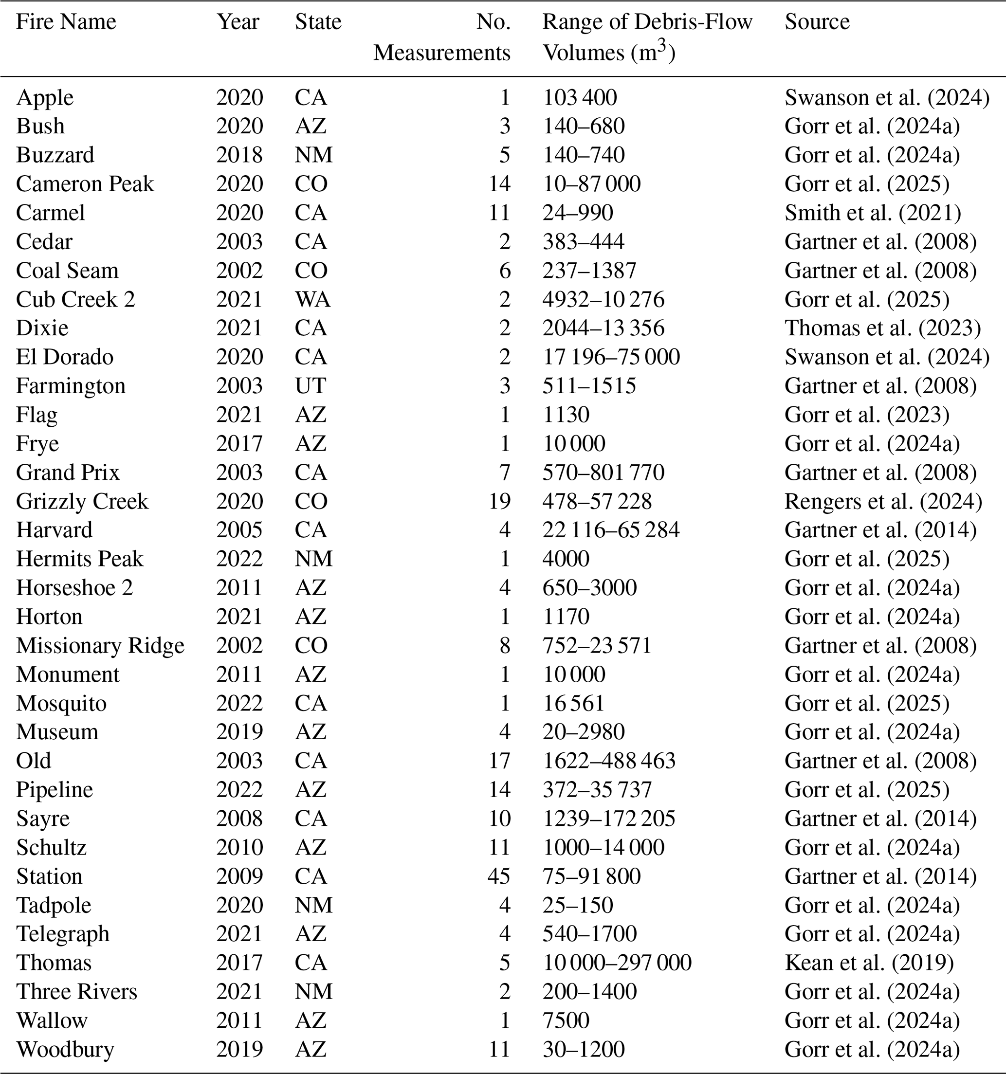
Table 1 Fire and associated debris-flow information. Fire information includes the fire name, year of occurrence, and location, including Arizona (AZ), California (CA), Colorado (CO), New Mexico (NM), Utah (UT), and Washington (WA). Debris-flow information includes the number of volume measurements for each fire, the range of associated sediment volumes, and the original sources of the volume measurements.

2 Data

2.1 Debris-flow volumes

We compiled a database of 227 postfire debris-flow volumes from across the western United States (Fig. 1) to develop the new volume model introduced in this study. Roughly 85 % of the database (192 of 227 volumes) consists of previously published postfire debris-flow volumes from Arizona (Gorr et al., 2024a); California (Gartner et al., 2008, 2014; Kean et al., 2019; Smith et al., 2021; Swanson et al., 2024), Colorado (Gartner et al., 2008; Rengers et al., 2023), New Mexico (Gorr et al., 2024a), and Utah (Gartner et al., 2008). We collected the remaining 15 % of volumes (35) from sites in Arizona, northern California, Colorado, New Mexico, and Washington as part of this study (Table 1). All volumes represent the volume of sediment deposited downstream from the watershed outlet. We did not consider the volume of water mobilized by flows, nor any sediment that may have been mobilized and deposited upstream from the watershed outlet. This is consistent with the data used to develop previous postfire debris-flow volume models (e.g., Gartner et al., 2014; Gorr et al., 2024a).

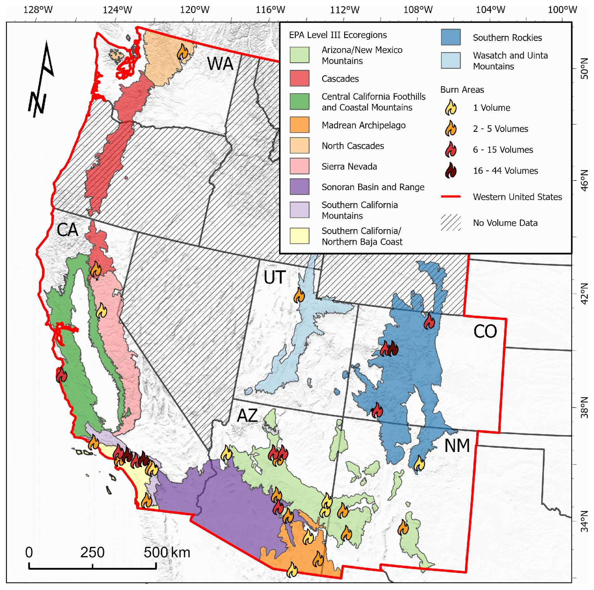
Figure 1 Map of the locations of the 34 burn areas included in this study. The burn areas span six states across the western United States (US), including Arizona (AZ), California (CA), Colorado (CO), New Mexico (NM), Utah (UT), and Washington (WA), and 11 Environmental Protection Agency (EPA) Level III Ecoregions. The names of the ecoregions shown in this figure are derived directly from the EPA (U.S. Environmental Protection Agency, 2013). Basemap credits: United States Geological Survey The National Map: 3D Elevation Program, United States Geological Survey Earth Resources Observation & Science Center: GMTED2010.

The volumes that we compiled were collected using a range of field and remote-sensing techniques. Most volumes were measured using some variation of the field survey methods outlined in Gorr et al. (2024a). In short, measurements of deposit area and average thickness were made in the field and then multiplied to determine debris-flow volume (e.g., Gorr et al., 2024a; Swanson et al., 2024). Other methods used to measure postfire debris-flow volume in the field included surveys of closely spaced channel cross-sections (e.g., Gartner et al., 2008) and counting the number of trucks filled with sediment when emptying a debris-retention basin (truck counts) (Gartner et al., 2014). The remaining volumes were measured primarily using remote-sensing techniques. Most commonly, these volumes were calculated using digital elevation models (DEM) of difference (DoD) that were generated by differencing pre-event and post-event light detection and ranging (lidar) (Smith et al., 2021; Rengers et al., 2024; Swanson et al., 2024). In other cases, high-resolution aerial imagery was used to help constrain the area of larger debris flows, and volume was calculated by multiplying the area by depth measurements made in the field (e.g., Gorr et al., 2024a).

Variations in the size of the debris-flow volumes included in this database, and the techniques used to measure them, mean that the uncertainty associated with each volume varies widely. Santi (2014) determined that the uncertainty associated with deposit boundary and thickness measurements, the most commonly used method to measure volumes in this database, was −25 % to +35 % for small debris flows (∼ 1500 m³), −28 % to +30 % for medium debris flows (∼ 15 000 m³), and −9 % to +17 % for large debris flows (∼ 150 000 m³). Other field measurement techniques, such as truck counts and channel cross-section surveys, have a lower degree of uncertainty, but still vary between −25 % and +20 %, depending on debris-flow size (Santi, 2014). The uncertainty associated with volumes measured by remote-sensing techniques are less constrained, but we estimate that the volumes calculated by lidar differencing have an uncertainty of −14 % to +14 %, based on a ± 10 cm level of detection (LoD) (Rengers et al., 2024). Overall, given the wide range of debris-flow sizes and measurement techniques included in the volume database, we conservatively estimate the uncertainty associated with these volume measurements to be ± 25 %.

The volume database includes data from 195 watersheds from 34 burn areas across six states in the western United States, a region we define as the states of Arizona, California, Colorado, Idaho, Montana, Nevada, New Mexico, Oregon, Utah, Washington, and Wyoming (Fig. 1; Table S1 in the Supplement). Specifically, the volume database includes volumes from Arizona, California, Colorado, New Mexico, Utah, and Washington (Fig. 1). The burn areas included in this study range in size from 4.2 to 3965 km² and span a wide range of climatological settings. The mean annual precipitation at the burn areas ranges from 396 to 1343 mm, and the mean annual temperature ranges from 3.7 to 17.8 °C (PRISM Climate Group, 2025) (Table S1).

The burn areas are also geographically and ecologically diverse, as they span 11 Level III ecoregions, or areas where ecosystems and ecosystem components, including geology, vegetation, climate, and hydrology, are generally similar (U.S. Environmental Protection Agency, 2013) (Fig. 1). The names of the ecoregions presented here are derived directly from U.S. Environmental Protection Agency (2013). The Arizona/New Mexico Mountains ecoregion, which is characterized by steep foothills, mountains, and dissected plateaus (Wilken et al., 2011), contains 12 burn areas. Grassland, chaparral, and pinyon-juniper and oak woodlands grow at lower elevations in this ecoregion, whereas ponderosa pine and mixed-conifer forests are common at higher elevations (Wilken et al., 2011). The Southern California Mountains ecoregion contains seven burn areas (Fig. 1). This ecoregion contains the high-elevation Transverse Ranges, which serve as a buffer between a coastal Mediterranean climate to the west and a dry, desert climate to the east. Chaparral and oak woodlands are the predominant vegetation communities in this region, although coniferous forests are found at higher elevations (Griffith et al., 2016). The Southern Rockies ecoregion, which includes most of western Colorado, as well as parts of southern Wyoming and northern New Mexico, contains an additional five burn areas (Fig. 1). It consists primarily of steep, high-elevation mountain ranges, with some intermontane valleys, and the dominant vegetation communities vary based on a steep elevation gradient. Grasslands and shrublands are common at lower elevations, ponderosa pine, aspen, juniper, and oak forests at middle elevations, mixed-conifer forests at higher elevations, and alpine vegetation at the highest elevations (Wilken et al., 2011; Drummond, 2012). The remaining 12 burn areas are spread across an additional eight ecoregions that contain between one to 3 burn areas each (Fig. 1). These ecoregions range from the high, rugged mountains and dense coniferous forests of the North Cascades ecoregion to the low, broad basins and microphyllous scrubland of the Sonoran Basin and Range ecoregion (Wilken et al., 2011).

2.2 Rainfall, topography, and fire severity data

In addition to debris-flow volume data, we also collected data related to rainfall, terrain, and fire characteristics to calculate 36 potential predictor variables for use in the development of the new volume model, as described in more detail in Sect. 3.1. We collected rainfall data for every debris-flow-producing storm using a series of rain gages located near watersheds with volume measurements. The rain gages we used were installed and maintained by local, state, and federal government agencies including, but not limited to, the Los Angeles County Department of Public Works (Gartner et al., 2014), Arizona Department of Water Resources (Gorr et al., 2024a), U.S. Forest Service (Gorr et al., 2024a), and the USGS (Gartner et al., 2014), as well as universities (Smith et al., 2021), and private consulting firms (Gorr et al., 2024a). To ensure that the recorded rainfall was representative of the debris-flow-producing storms, we used rain gages located within 4 km of watersheds with debris-flow volume measurements, as suggested by Staley et al. (2017). Most rain gages, however, were located within 2 km of the debris-flow-producing watersheds. We could attribute most debris-flow volumes to a single storm, but when there were multiple storms prior to a volume measurement, we followed the methods of Gartner et al. (2014) and attributed the volume to the most intense storm that occurred between the assumed debris-flow initiation date and the volume measurement. We defined individual storms as events that were separated by at least 8 h without rainfall (Staley et al., 2020).

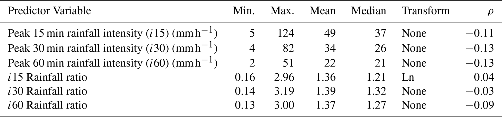
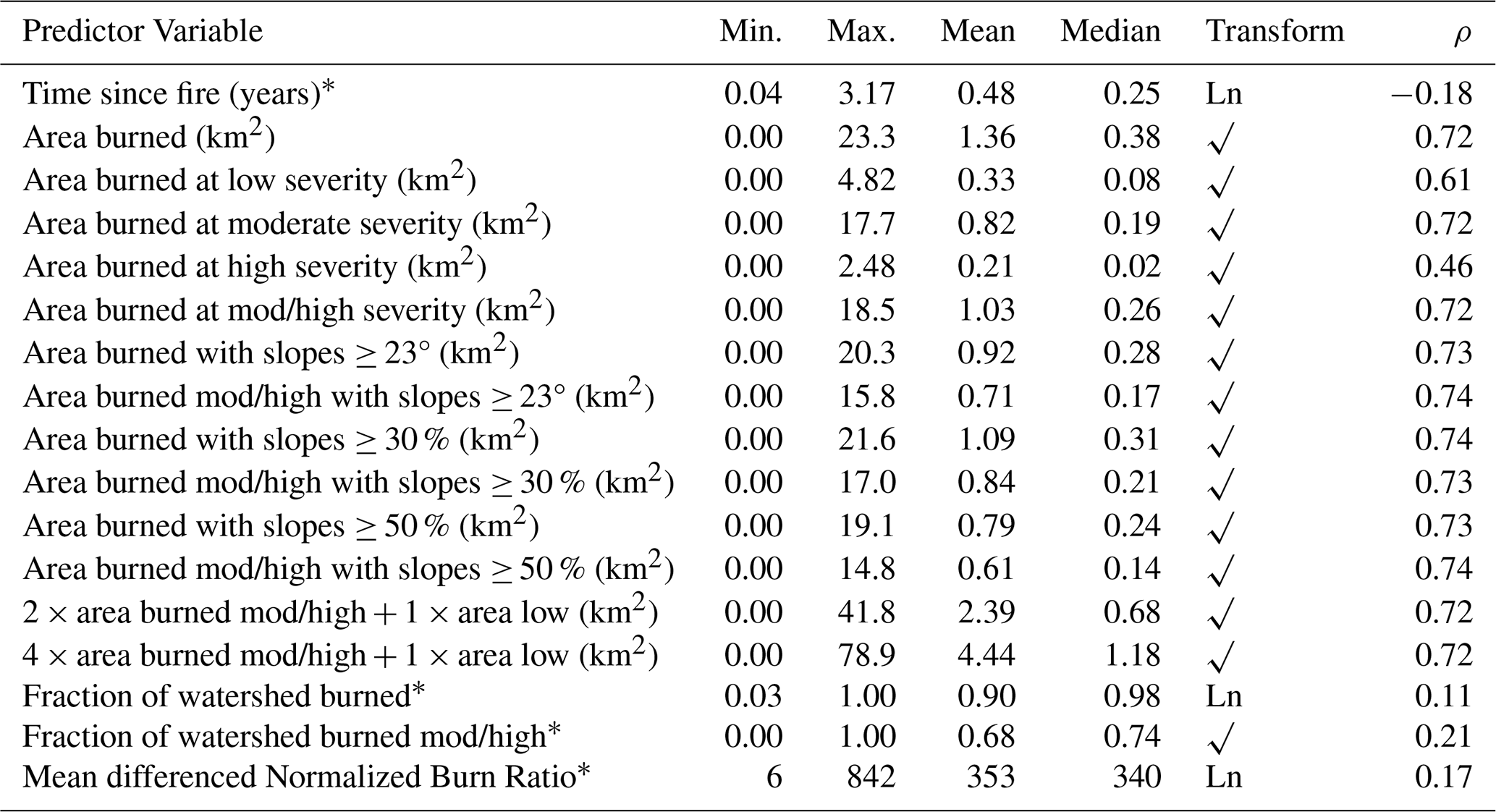
Table 2 Summary statistics for rainfall predictor variables, as well as the transformation of each variable (e.g., no transformation (None) or natural log (Ln)) that yielded the most linear relationship with debris-flow volume, which we determined using the Pearson product-moment correlation coefficient (ρ).

We used national datasets to calculate metrics related to terrain and fire characteristics for each debris-flow-producing watershed included in our database. Specifically, we resampled the $\mathrm{1}/\mathrm{3}$ arcsec seamless DEM dataset from the USGS 3D Elevation Program (3DEP) to create a series of 10 m resolution DEMs that we used to delineate watershed boundaries and calculate terrain metrics for each watershed. We manually defined the outlet of each watershed as the point immediately upstream from the debris-flow deposit used to calculate volume, ensuring that all terrain metrics only considered the watershed area that contributed to debris-flow volume. This also ensured consistency among metrics related to fire characteristics, which we calculated using data from the Monitoring Trends in Burn Severity (MTBS) program (Monitoring Trends in Burn Severity, 2025). MTBS provides information for all fires 405 ha and larger in the western United States that burned from 1984 to present, including ignition date, fire severity, and differenced Normalized Burn Ratio (dNBR) data (Monitoring Trends in Burn Severity, 2025). The differenced Normalized Burn Ratio is a remote-sensing index that measures fire-induced changes in vegetation by comparing pre- and post-fire satellite imagery and is commonly used to classify burn severity (Parsons et al., 2010).

3 Methods

3.1 Calculation of predictor variables

We calculated 36 potential predictor variables for use in model development: six rainfall variables, 13 terrain variables, and 17 variables related to fire characteristics. We analyzed six variables related to peak rainfall intensity and rainfall ratios (Table 2) because previous work indicates that hourly or sub-hourly rainfall intensity data can be used to more accurately constrain postfire debris-flow volume (e.g., Pak and Lee, 2008; Gartner et al., 2014; Gorr et al., 2024a). We define a rainfall ratio as a recorded rainfall metric normalized by that same metric associated with a 1 year recurrence interval storm at a given location (Cavagnaro et al., 2025a). For example, we define the rainfall ratio of the peak rainfall intensity measured over a 15 min duration (i15) as the recorded i15 normalized by the i15 associated with a 1 year recurrence interval storm at a given watershed. Similarly, we define the rainfall ratios of the peak rainfall intensity measured over 30 min (i30) and 60 min (i60) durations as the recorded i30 or i60 normalized by the i30 or i60 associated with a 1 year recurrence interval storm at a given watershed.

We selected a 1 year recurrence interval to calculate rainfall ratio, as postfire debris flows in the western United States are generated by storms with a 1 year recurrence interval, on average (Staley et al., 2020). When available, we used National Oceanic and Atmospheric Administration (NOAA) Atlas 14 precipitation frequency data (Bonnin et al., 2011; Perica et al., 2013, 2014) to determine the i15, i30, and i60 of 1 year recurrence interval storms at each debris-flow-producing watershed. For one burn area where Atlas 14 data were not available (Cub Creek 2), we used NOAA Atlas 2 data (Miller et al., 1973) to estimate the i15, i30, and i60 of a 1 year recurrence interval storm. When known, we determined the 1 year recurrence interval values at the location of the rain gage where rainfall was recorded. If we did not know the location of the rain gage (i.e., the coordinates of the gage were not provided by a previous study), we used the 1 year recurrence interval rainfall associated with the centroid of the associated watershed. We considered rainfall ratio metrics because previous studies have identified a relationship between postfire debris-flow likelihood and rainfall ratio (referred to as “rainfall anomaly” in Cavagnaro et al., 2025a), suggesting that there may also be a relationship with postfire debris-flow volume.

Table 3 Summary statistics for watershed terrain predictor variables, as well as the transformation of each variable (e.g., natural log (Ln) or square root (√)) that yielded the most linear relationship with debris-flow volume, which we determined using the Pearson product-moment correlation coefficient (ρ).

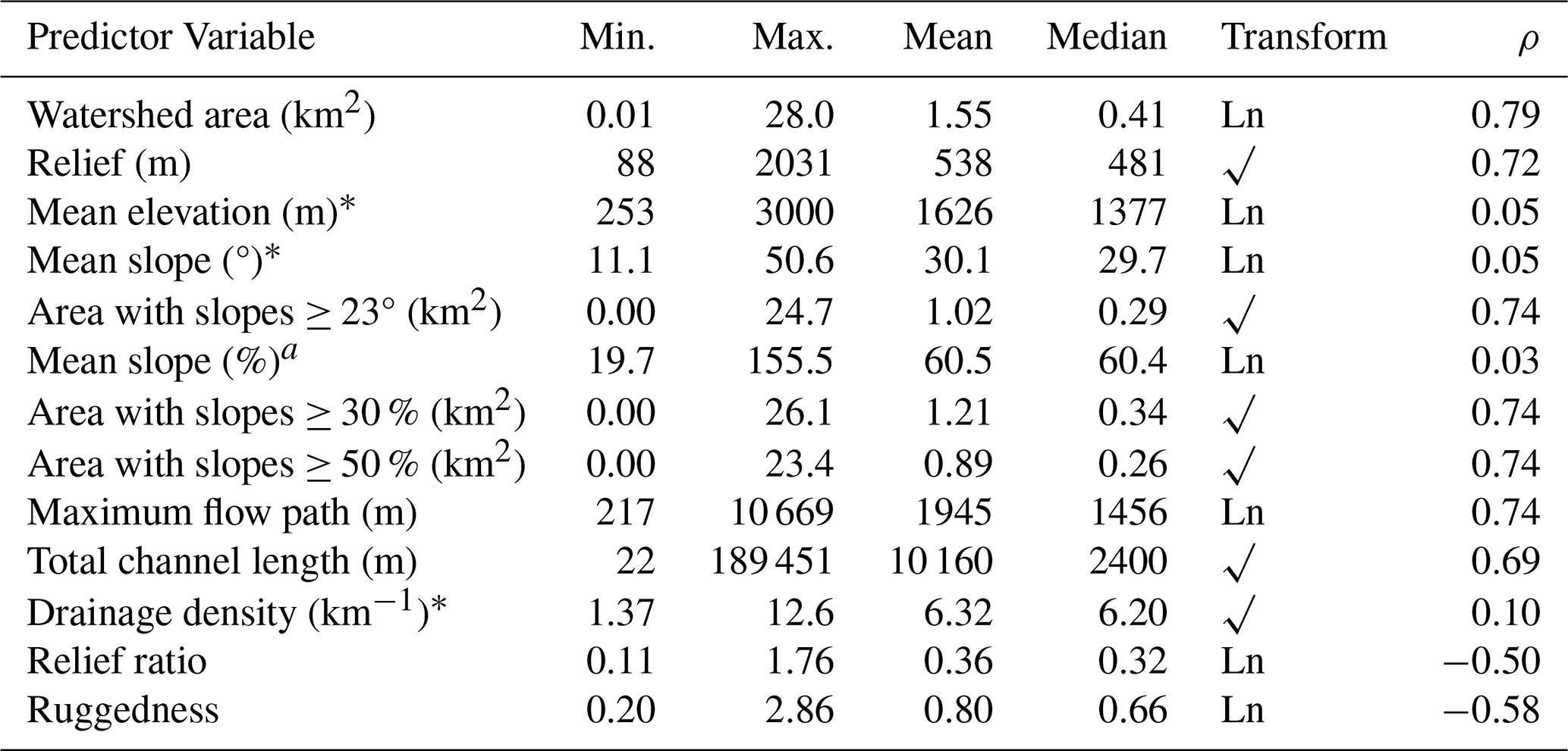
^∗ Variable removed because it was not linearly related to volume.

We also calculated 13 terrain variables that previous studies found were correlated with postfire debris-flow volume (Gartner et al., 2014; Wall et al., 2023; Gorr et al., 2024a) for all 195 debris-flow-producing watersheds using ArcGIS Pro 3.3.0 (Table 3). Here we define relief (Table 3) as the difference between the maximum elevation and minimum elevation within a watershed, maximum flow path as the longest flow path within a watershed, as measured from the watershed outlet to the top of the drainage divide, and total channel length as the combined length of all channels within a watershed. Drainage density is defined as the total channel length divided by the watershed area, relief ratio as the length of the maximum flow path divided by watershed relief, and ruggedness, also known as the Melton ratio, as watershed relief divided by the square root of watershed area. We used 10 m DEMs to calculate these variables because this was the highest resolution data available for every watershed. Ensuring consistency across sites was necessary, as several of the terrain variables that we calculated (e.g., slope) were dependent on DEM resolution (Smith et al., 2019).

Table 4 Summary statistics for fire predictor variables, as well as the transformation of each variable (e.g., natural log (Ln) or square root (√)) that yielded the most linear relationship with debris-flow volume, which we determined using the Pearson product-moment correlation coefficient (ρ).

^∗ Variable removed because it was not linearly related to volume

We calculated another 17 variables for each watershed related to fire characteristics (Table 4) that previous studies have found to be correlated with postfire debris-flow volume using data from MTBS (Gartner et al., 2014; Wall et al., 2023; Gorr et al., 2024a). We define time since fire (Table 4) as the time between the date of fire ignition and the date of debris-flow initiation. Mean dNBR is the only fire variable we considered that has not been explored by previous volume studies (e.g., Gartner et al., 2014; Wall et al., 2023; Gorr et al., 2024a). We included it in this analysis because it has been identified as an important control on postfire debris-flow likelihood (Staley et al., 2017), and because it provides an objective measure of how severely a watershed has been affected by fire.

3.2 Model development

3.2.1 Initial screening of predictor variables

After identifying 36 potential predictor variables related to rainfall (Table 2), watershed terrain (Table 3), and fire characteristics (Table 4), we used a multiple linear regression analysis to develop a model for predicting postfire debris-flow volume in the western United States. Multiple linear regression is a statistical technique that uses multiple predictor variables to estimate the value of a response variable (debris-flow volume) following the general form:

$$\begin{array}{}\text{(1)}& y={\mathit{\beta }}_{\mathrm{0}}+{\mathit{\beta }}_{\mathrm{1}}{x}_{\mathrm{1}}+{\mathit{\beta }}_{\mathrm{2}}{x}_{\mathrm{2}}+\mathrm{\dots }+{\mathit{\beta }}_k{x}_k+\mathit{\epsilon }\end{array}$$

where y is the response variable, β₀ is the intercept, x_i is the ith predictor variable, β_i is the slope coefficient for the ith predictor variable, x_k and β_k are the kth predictor variable and the slope coefficient for the kth predictor variable, respectively, and ε is the error term.

We started the model development process by ensuring that each potential predictor variable was linearly related to debris-flow volume, as a linear relationship between predictor variable and response variable is a requirement of multiple linear regression (Helsel et al., 2020). First, we used the Pearson product-moment correlation coefficient (ρ) to quantify the relationship between the response variable and each predictor variable. We then took the square root and natural log of the response and predictor variables to assess whether transforming one, or both, variables resulted in a more linear relationship between the two. This process resulted in nine correlation coefficients, representing the relations between the response variable and the predictor variable after applying each of 3 transformations (no transform, square root, and natural log) to both variables. Using this information, we selected the transformations that yielded the highest value of ρ, and thus the most linear relationship between the variables (Tables 2–4). Additionally, because ρ can be heavily influenced by outliers or a curved relationship between response and predictor variables (Helsel et al., 2020), we used scatter plots to visually confirm that debris-flow volume and each predictor variable exhibited a linear relationship. Using these plots, we determined that predictor variables that had a ρ value between −0.3 and 0.3 did not exhibit a convincing linear relationship with debris-flow volume. As a result, we removed these variables from our analysis (Tables 3 and 4).

We made an exception to the requirement that each predictor variable be linearly related to debris-flow volume for variables related to rainfall. Although none of the rainfall variables explored here had a correlation coefficient stronger than ± 0.3 (Table 2), we did not remove them from our analysis, as previous studies have found that including a rainfall variable can result in more accurate estimates of postfire debris-flow volume (e.g., Pak and Lee, 2008; Gartner et al., 2014; Gorr et al., 2024a). For instance, Gorr et al. (2024a) found that volume models that contained a rainfall variable considerably outperformed those that did not, despite a weak relationship between the rainfall variables they considered and debris-flow volume. We attribute the weak relationship between rainfall variables and debris-flow volume in this study to uncertainty in the rainfall data. Though we only used data from rain gages within 4 km of debris-flow-producing watersheds, spatial variations in rainfall may have still resulted in substantial differences between what was measured by a rain gage and actual rainfall conditions in the watershed (Fig. S1 in the Supplement). This situation was likely more common in states like Arizona, Colorado, and New Mexico, where most debris flows initiate as the result of highly localized convective storms (e.g., Cannon et al., 2008; Gorr et al., 2023; McGuire et al., 2024b). However, this uncertainty and lack of linearity is in line with that of rainfall data used in previous volume studies (e.g., Gartner et al., 2014; Gorr et al., 2024a), so we did not remove any rainfall variables from our analysis based on the linear relationship requirement. As a result, we were left with 28 potential predictor variables for model development.

3.2.2 Predictor variable selection and model calibration

We selected the predictor variables for the new volume model using a multi-step procedure designed to maximize model performance, minimize the number of predictor variables used, and ensure that the final model met all requirements for multiple linear regression. Because we considered 28 predictor variables, there were 2²⁸ potential variable combinations that we could have evaluated. Instead of considering all 2²⁸ potential variable combinations, we grouped the variables into 3 bins (rainfall, terrain, and fire) and only considered models that contained one variable from each bin (n=702). Following the methods outlined below, we fit each of the 702 models, selected those that met the requirements of multiple linear regression (i.e., had residuals that were normally distributed and had a constant variance) (Helsel et al., 2020), identified a subset of similarly performing top models (n=29), and made final variable selection based on additional multiple linear regression requirements and the relative frequency of occurrence of predictor variables within the top model subset.

We started the variable selection process by separating each of the remaining 28 predictor variables into 3 bins (six rainfall variables, nine terrain variables, and 13 fire variables) and only considered models that selected one variable from each bin to prevent multicollinearity. Multicollinearity occurs when one predictor variable is closely related to another, and it can result in unrealistically large slope coefficients and illogical relationships between predictor and response variables (Eq. 1), negatively impacting model performance (Alin, 2010; Helsel et al., 2020). Separating the predictor variables into bins reduced the likelihood of selecting two variables that exhibited multicollinearity (e.g., watershed area with slopes ≥ 23° and watershed area with slopes ≥ 30 %). This process yielded 702 unique combinations of rainfall, terrain, and fire predictor variables. We then fit a multiple linear regression model to each combination using the Statistics and Machine Learning Toolbox in MATLAB R2024b, resulting in 702 unique, three-variable models.

After independently fitting all 702 models, we evaluated each to ensure they met the following requirements of multiple linear regression: that the residuals were normally distributed and that the residuals had a constant variance (Helsel et al., 2020). These requirements ensure valid hypothesis tests and reliable confidence and prediction intervals for the model (Helsel et al., 2020). We used the Anderson–Darling (AD) test (Anderson and Darling, 1954) to assess the normality of model residuals, and the Brown–Forsythe (BF) test (Brown and Forsythe, 1974) to assess the variance of the residuals. The null hypothesis for the AD test is that the residuals follow a normal distribution. Therefore, an AD p-value > 0.05 indicates that the null hypothesis cannot be rejected and that the residuals are normally distributed. The null hypothesis for the BF test is that the residuals have a constant variance, so a BF p-value > 0.05 means that the null hypothesis cannot be rejected and that there is a constant variance in the residuals. To ensure our final model met these requirements of multiple linear regression, we removed 570 models that did not pass the AD and/or BF tests from consideration, leaving 132 models for further analysis.

After removing the models that did not fit our statistical requirements, we evaluated the performance of the remaining 132 models against the entire volume database using metrics including R² and root mean square error (RMSE). Higher R² values and lower RMSE values reflected better model performance. We also calculated the percentage of volumes predicted within an order of magnitude by each model, as having a first order estimate of debris-flow magnitude is useful for rapid hazard assessment scenarios. We used these metrics to further reduce the number of models we considered during our final model selection process by removing all models where the R² and RMSE values were not within 10 % of those of the best-performing model. This resulted in 29 models to consider for final evaluation.

From the remaining 29 models, we selected one final model using several factors in addition to the metrics outlined above. First, we determined how often each rainfall, terrain, and fire variable appeared in the 29 best-performing models, and prioritized models that used more commonly selected variables. Given the similar quantitative performance of the remaining 29 models, we interpreted variables that appeared more frequently as those that were more important for constraining postfire debris-flow volume using our dataset. We also ensured that there was no multicollinearity between the selected predictor variables for each model using the variance inflation factor (VIF) (Marquardt, 1970). We interpreted VIF values over 10 as indicative of a strong relationship between predictor variables (Helsel et al., 2020). We used a p-value of 0.1 to assess whether the predictor variables included in each model were statistically significant and removed any models that contained one or more predictor variables with a p-value > 0.1 from consideration. Finally, we assessed whether the predictor variables included in each model fit our conceptual understanding of postfire debris-flow growth. For example, it is well-established that more intense rainfall tends to produce larger debris-flow volumes (e.g., Gartner et al., 2014; Gorr et al., 2024a), so we did not consider models that exhibited a negative relationship between rainfall intensity and volume. Using these considerations, in addition to the quantitative performance metrics, we selected a final model for predicting postfire debris-flow volume in the western United States, which we refer to hereafter as the western United States (WEST) model.

3.3 Model validation

We ensured the WEST model was not overfit using iterated fivefold cross validation (Kohavi, 1995), a method that has been used to validate previous postfire debris-flow volume models (e.g., Gorr et al., 2024a). We started this process by randomly separating the volume database into five similarly sized groups, four of which we classified as the training dataset and one as the testing dataset. We then fit the model on the training dataset and evaluated its performance against the testing dataset using R² and RMSE. We repeated this process. four more times so that each group of volumes was used as part of the training dataset four times and as the testing dataset once, resulting in five R² and RMSE values that we averaged to determine a mean R² and RMSE for that iteration of the fivefold cross validation. Then, we started the entire process over again by randomly splitting the volume database into five new groups. In total, we completed 20 iterations of fivefold cross validation to more robustly evaluate model performance when applied to different subsets of data. This process yielded 100 distinct groups of volume data that were used for both training and testing, as well as 20 averaged R² and RMSE values. We once again averaged the mean R² and RMSE values to determine a single cross-validated (CV) R² and RMSE, which we used to evaluate how well the model performed against unseen data. We also assessed the distribution of the R² and RMSE values associated with all 100 folds to determine how generalizable the model was to different subsets of volume data. We interpreted CV R² and RMSE values similar to the R² and RMSE of the WEST model trained on the entire dataset as an indication that the model was not overfit, and a narrow range of R² and RMSE values as an indication that the model was not overly sensitive to volumes from specific geographic regions.

3.4 Comparison with existing models

We compared the performance of the WEST model against the performance of 3 existing postfire debris-flow volume models: the Emergency Assessment volume (EAV) model (Gartner et al., 2014), the Intermountain West (IMW) volume model (Wall et al., 2023), and the V1 volume model (Gorr et al., 2024a). Although other methods for predicting postfire debris-flow volume exist (Santi and Morandi, 2013; Pelletier and Orem, 2014; Donovan and Santi, 2017), we selected the EAV, IMW, and V1 models, in particular, for comparison because they were developed for the purpose of postfire hazard assessment using, at least in part, subsets of volume data from the larger volume database used in this study (Gartner et al., 2014; Wall et al., 2023; Gorr et al., 2024a). However, unlike the WEST model, which was developed using data from across the western United States (Fig. 1), these models were developed using data from more specific geographic regions, including southern California (Gartner et al., 2014), the Intermountain West, defined as the states of Arizona, Colorado, Idaho, Montana, Nevada, New Mexico, Utah, and Wyoming (Wall et al., 2023), and the Southwest, defined as the states of Arizona and New Mexico (Gorr et al., 2024a). Note that the Southwest is a smaller region within the larger Intermountain West, and both regions include the states of Arizona and New Mexico. The IMW model was developed for a broad region that includes Arizona and New Mexico (Wall et al., 2023), whereas the V1 model was developed for use in Arizona and New Mexico, specifically (Gorr et al., 2024a). We compared the WEST model to these 3 regional models to further evaluate model performance against existing methods for constraining postfire debris-flow volume.

We evaluated and compared the performance of each of the models when applied to the entire western United States database. Additionally, to more fairly compare the existing models to the WEST model, we also evaluated the performance of each model when applied to subsets of data from the regions for which the existing models were developed: southern California (Gartner et al., 2014), the Intermountain West (Wall et al., 2023), and the Southwest (Gorr et al., 2024a). The southern California dataset consisted of 93 debris-flow volumes from the Transverse Ranges (Table 1), the Intermountain West dataset of 118 volumes from the states of Arizona, Colorado, New Mexico, and Utah, and the Southwest dataset of 68 volumes from Arizona and New Mexico (Table 1). By assessing the performance of each model against these subsets of volume data, we were able to evaluate how the WEST model performed against regional models when applied to the regions in which those models were developed. We also evaluated how each of the models performed against volumes from data-limited regions, which we define as regions where there is currently not enough volume data to develop a regional volume model. The data-limited dataset included 19 total volumes: 14 from northern California, 3 from Utah, and 2 from Washington (Table S2 in the Supplement).

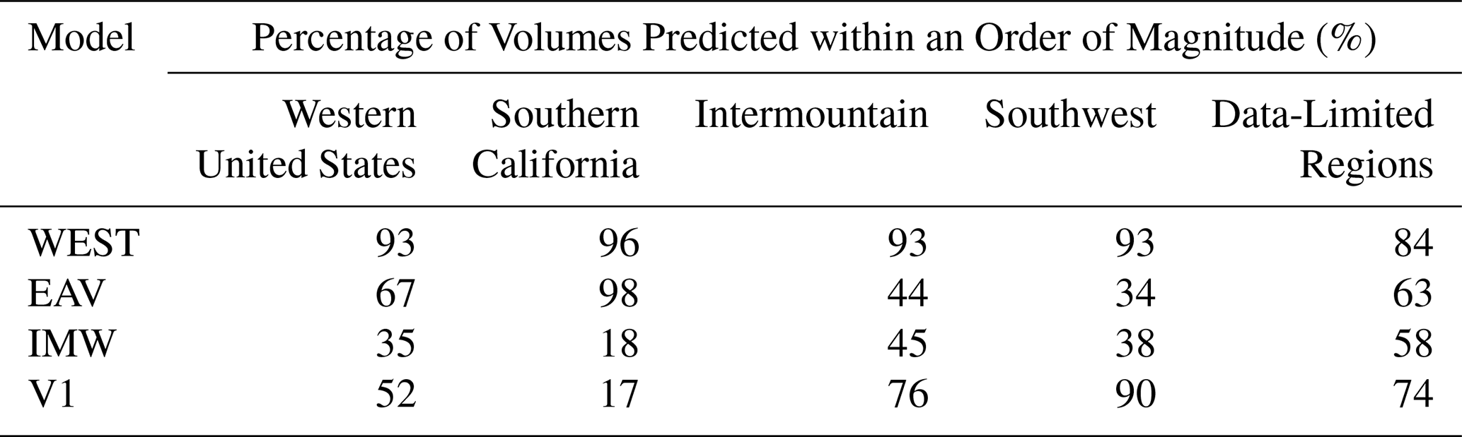
We used multiple metrics to evaluate the performance of each model across the five subsets of volume data. We visually assessed the goodness of fit of each model by plotting the probability density function of model residuals and quantified it by calculating the mean (μ) and standard deviation (σ) of the residuals. Residual mean values closer to zero and smaller σ values indicate better model performance. We also calculated the median absolute error (MAE) and the percentage of volumes predicted within an order of magnitude to further assess model performance. Because all four volume models were developed in natural logarithmic space (Gartner et al., 2014; Wall et al., 2023; Gorr et al., 2024a), we present μ and σ values in their natural log transformed form. However, we present the MAE and percentage of volumes predicted within an order of magnitude in dimensional space for better interpretability.

4 Results

4.1 WEST model

Using the methods outlined in Sect. 3.2, we selected one model for predicting postfire debris-flow volume in the western United States. The WEST model predicts the volume of sediment deposited by postfire debris flows using the equation:

$$\begin{array}{}\text{(2)}& \ln V=\mathrm{7.56}+\mathrm{0.20}{i}_{\mathrm{30}\text{rr}}+\mathrm{0.75}\ln a+\mathrm{1.11}\sqrt{{\mathrm{mh}}_{\mathrm{50}}}\end{array}$$

where V is debris-flow volume (m³), i_30rr is the i30 rainfall ratio, a is watershed area (km²), and mh₅₀ is watershed area burned at moderate or high severity with slopes ≥ 50 % (∼ 27°) (km²). The WEST model had an R² = 0.66 and a RMSE = 1.31, both of which were the best among the 29 final models discussed in Sect. 3.2.2 (Tables S3 and S4 in the Supplement). The variance inflation factor (VIF) for each predictor variable in the WEST model was less than three, indicating that there was no multicollinearity, and the p-value for all 3 predictor variables was < 0.1, indicating that each was statistically significant. Note that although we selected the WEST model as the final model for this study using the criteria outlined above, many of the final 29 models offer similar performance metrics (Table S3) and may be viable alternatives to the WEST model in some scenarios.

The WEST model overpredicted 48 % of volumes in the database and underpredicted the remaining 52 % (Fig. 2). It predicted 41 % of volumes within 1000 m³, 75 % within 10 000 m³, and 98 % within 100 000 m³ of what was observed. It also predicted 93 % of volumes within an order of magnitude (Fig. 2). Additionally, the relations among debris-flow volume and each of the predictor variables selected for inclusion in the WEST model agreed with our conceptual understanding of postfire debris-flow growth, as more intense rainfall, larger watersheds, steeper slopes, and higher burn severity yielded greater sediment volumes (Eq. 2).

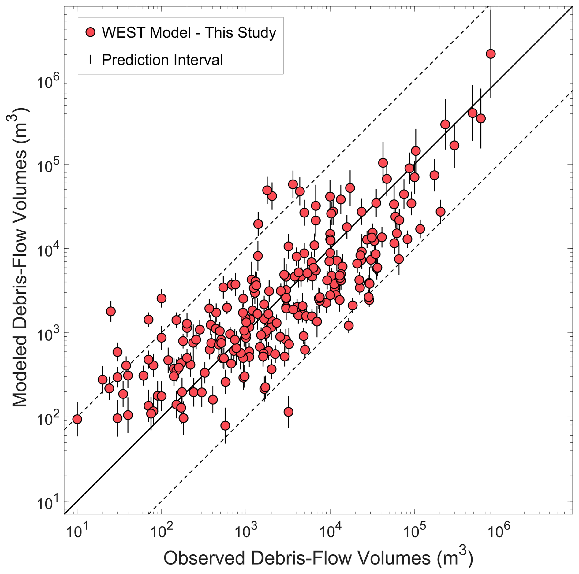
Figure 2 A comparison between the observed volume of all 227 postfire debris flows and the corresponding volume predicted by the western United States (WEST) model. Vertical lines represent the 95 % prediction interval associated with each point. The thick, black line is a 1:1 line, and the thin, dashed lines represent an order of magnitude envelope.

Results of the cross-validation (CV) evaluation indicated that the WEST model was not overfit and was not overly sensitive to volumes from any particular geographic region (Fig. S2 in the Supplement). The CV R² and RMSE values were 0.63 and 1.32, respectively, closely matching the R² (0.66) and RMSE (1.31) values of the WEST model trained on the entire volume database. This demonstrated that the model generalized well to unseen data. Additionally, the distributions of the 100 fold-level R² and RMSE values were relatively narrow (Fig. S2), with standard deviations of 0.08 and 0.13, respectively, indicating that, although there was some fold-to-fold variability, most splits produced broadly similar performance, regardless of the geographic distributions of the volumes. Furthermore, the 20 mean R² and RMSE values (one associated with each iteration of fivefold cross validation) varied only slightly (Fig. S2), providing additional evidence that model performance was stable across random splits of the volume database.

Table 5 Residual means for the western United States (WEST), Emergency Assessment volume (EAV), Intermountain West (IMW), and V1 models (subset by region).

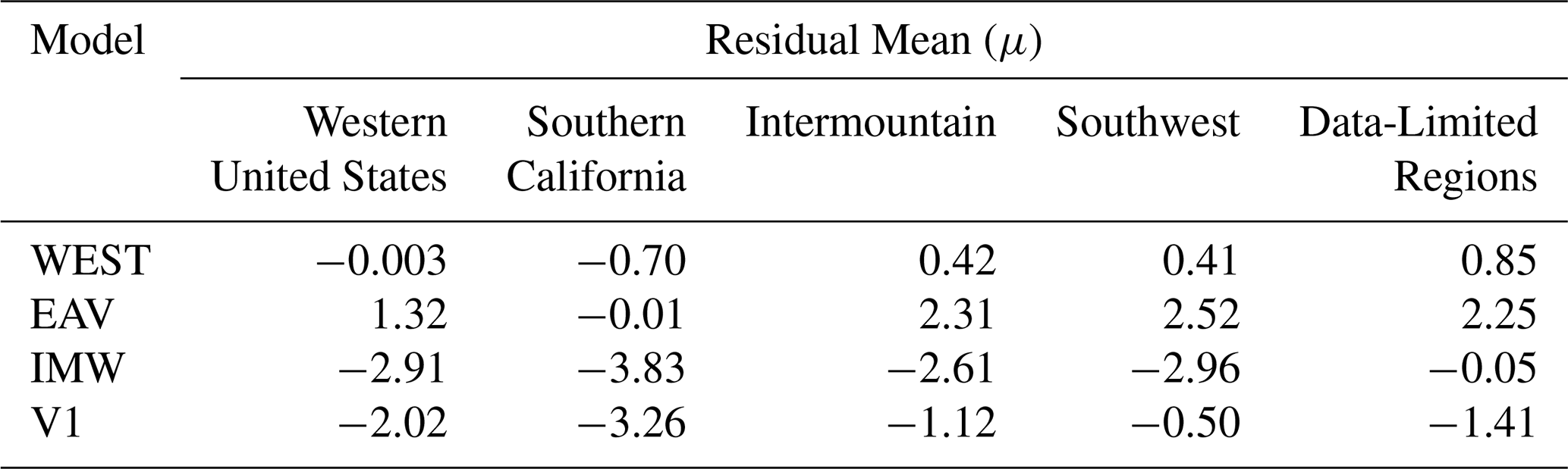
Table 6 Standard deviation of the residuals for the western United States (WEST), Emergency Assessment volume (EAV), Intermountain West (IMW), and V1 models (subset by region).

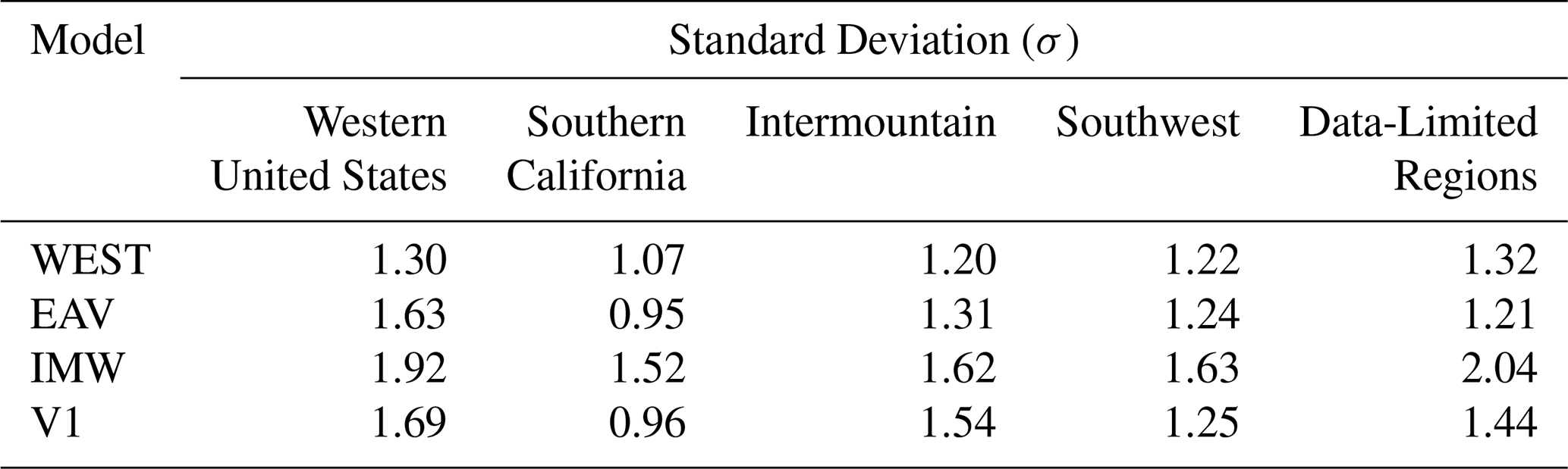
Table 7 Median absolute errors for the western United States (WEST), Emergency Assessment volume (EAV), Intermountain West (IMW), and V1 models (subset by region).

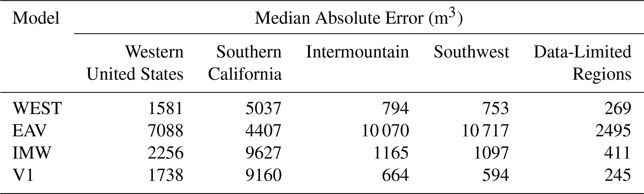
Table 8 Percentage of volumes predicted within an order of magnitude by the western United States (WEST), Emergency Assessment volume (EAV), Intermountain West (IMW), and V1 models (subset by region).

4.2 Comparison with existing models

The WEST model outperformed the EAV (Gartner et al., 2014), IMW (Wall et al., 2023), and V1 (Gorr et al., 2024a) models when applied to the entire western United States volume database. Probability density functions of model residuals revealed that the WEST model provided the best fit between observed and modeled postfire debris-flow volumes in the western United States (Fig. 3). The WEST model had a residual mean (μ) nearly equal to zero (Table 5), indicating that it did not systemically overpredict or underpredict debris-flow volumes in the western United States (Fig. 3a). In contrast, the EAV model (Fig. 3b) had a residual mean greater than zero, and the IMW (Fig. 3c) and V1 (Fig. 3d) models had residual means less than zero (Table 5), revealing that they tended to overestimate and underestimate postfire debris-flow volumes in this dataset, respectively. The WEST model also had the lowest standard deviation (σ) of all four models (Table 6), indicating the variability of the residuals was lower compared to the other 3 models. Finally, the WEST model had the lowest MAE (Table 7) and predicted the greatest percentage of volumes within an order of magnitude (Table 8), further indicating that it provided the best fit between modeled and observed volumes in the western United States.

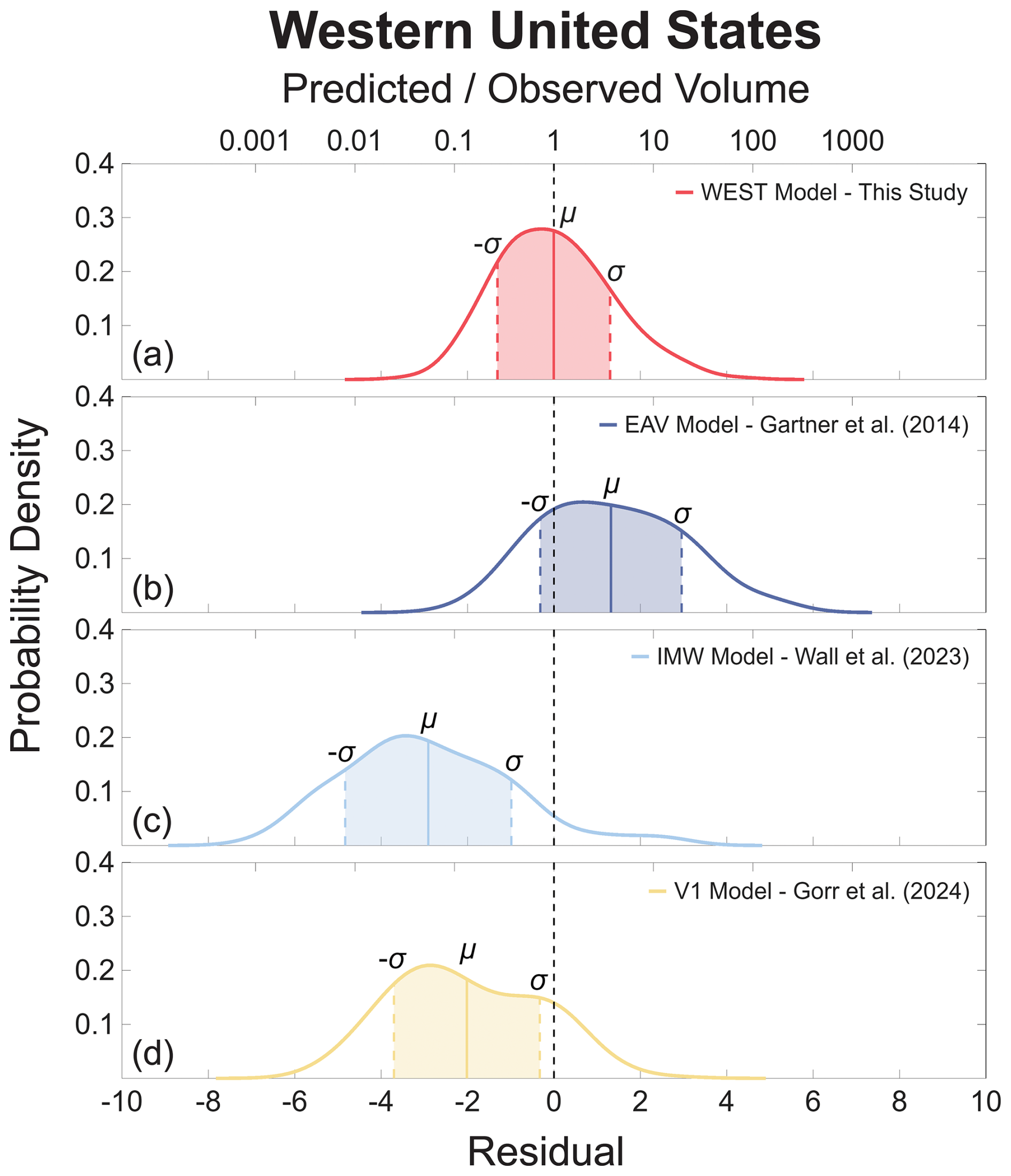
Figure 3 Probability density functions for the residuals of the (a) western United States (WEST), (b) Emergency Assessment volume (EAV), (c) Intermountain West (IMW), and (d) V1 models when applied to the entire western United States dataset.

The WEST model also performed well relative to existing models, when evaluated against subsets of data from regions where the other volume models were developed, including southern California (Fig. S3 in the Supplement), the Intermountain West (Fig. S4 in the Supplement), and the Southwest (Fig. S5 in the Supplement). In southern California, the WEST model was the second best-performing model, just behind the EAV model, which was developed for use in this region. Although the EAV model had a lower MAE (Table 7) and predicted a higher percentage of volumes within an order of magnitude (Table 8), the difference in performance between the EAV and WEST models was marginal, especially when compared to the IMW and V1 models (Fig. S3). The IMW and V1 models both had MAE values nearly double that of the EAV and WEST models (Table 7) and predicted less than 20 % of southern California volumes within an order of magnitude (Table 8). Both models also tended to substantially underpredict debris-flow volumes in southern California, whereas the WEST model only slightly underpredicted volumes in this region, on average (Table 5). The EAV model neither systemically overpredicted nor underpredicted volumes in southern California, as evidenced by a residual mean value of −0.01 (Table 5).

In some scenarios, the WEST model even outperformed existing models in the regions for which they were developed, including the Intermountain West (Fig. S4) and the Southwest (Fig. S5). In the Intermountain West, the WEST model outperformed the IMW model (Fig. S4). It had a lower MAE (Table 7) than the IMW model and predicted a greater percentage of volumes within an order of magnitude (Table 8) in this region. Furthermore, the residual mean of the WEST model was closer to zero (Table 5) and its standard deviation was smaller than that of the IMW model (Table 6), which systemically underpredicted volumes in the Intermountain West (Fig. S4). The WEST model also outperformed both the EAV and V1 models in the Intermountain West, as the EAV model greatly overpredicted debris-flow volume, on average, and the V1 model underpredicted debris-flow volume, on average (Fig. S4). In the Southwest, the WEST model outperformed the V1 model, according to most metrics (Fig. S5). Although the V1 model had a slightly lower MAE (Table 7), the WEST model predicted a greater percentage of volumes in the Southwest within an order of magnitude (Table 8), had a smaller standard deviation (Table 6), and had a residual mean closer to zero (Table 5). The WEST model tended to slightly overpredict debris-flow volumes in the Southwest (Fig. S5a), whereas the V1 model tended to slightly underpredict volumes in this region (Fig. S5d). The EAV and IMW models, on the other hand, more severely overpredicted and underpredicted volumes in the Southwest, respectively (Fig. S5). Differences between the volumes predicted by these models and observed volumes in the Southwest routinely exceeded an order of magnitude (Table 8).

When applied to 19 postfire debris-flow volumes from data-limited regions, including northern California, Utah, and Washington, (Table S2), the WEST model again outperformed the EAV, IMW, and V1 models. The WEST model predicted the greatest percentage of volumes within an order of magnitude (Fig. 4; Table 8) and had one of the lowest MAE values (Table 7). Although the IMW model had the residual mean closest to zero (Table 5), it also had the largest standard deviation (Table 6), indicating high variability in the residuals compared to other models (Fig. 5). The WEST model slightly overpredicted volumes from data-limited regions but had the second lowest standard deviation of the four models (Table 6). The EAV model had a slightly lower standard deviation than the WEST model but overpredicted volumes from data-limited regions more substantially (Fig. 5b). Unlike the WEST and EAV models, the V1 model underpredicted volumes from data-limited regions, on average (Fig. 5d).

5 Discussion

We introduced a new empirical model for predicting postfire debris-flow volume in the western United States. This model, referred to as the WEST model, predicts the volume of sediment deposited by postfire debris flows as a function of i30 rainfall ratio, watershed area, and watershed area burned at moderate or high severity with slopes greater than or equal to 50 % (Eq. 2). It offers an improvement over existing volume models because it accounts for regional differences in rainfall characteristics with a rainfall ratio metric and because it was trained on a larger dataset of debris-flow volumes from across the western United States. Specifically, the WEST model outperforms 3 existing debris-flow volume models (Gartner et al., 2014; Wall et al., 2023; Gorr et al., 2024a) when applied to the entire western United States database (Fig. 3), as well as to subsets of data from the Intermountain West (Fig. S4), the Southwest (Fig. S5), and data-limited regions (Figs. 4 and 5). It also maintains a similar level of performance to that of a model developed for use in southern California when applied in that region (Fig. S3). These results indicate that the WEST model is more broadly applicable than existing volume models, particularly in data-limited regions, and that it may be a promising tool for postfire hazard assessment in the western United States.

5.1 Improvements over existing models

5.1.1 Rainfall ratio

The WEST model offers an improvement over existing volume models because it accounts for regional differences in rainfall intensity and because it was trained on the largest dataset of debris-flow volumes. The WEST model uses a rainfall ratio metric that normalizes for regional variations in rainfall and is consequently able to achieve equivalent performance to several models developed for different regions of the western United States using a single regression equation. Prior regional volume models, on the other hand, use rainfall intensity (e.g., Gartner et al., 2008, 2014; Gorr et al., 2024a), and are thus limited when applied to areas outside of their training datasets due to regional differences in the intensity of debris-flow-generating rainfall (e.g., Gorr et al., 2023, 2024a; Rengers et al., 2023, 2024). Previous studies have found that, although hourly (Pak and Lee, 2008) or sub-hourly (e.g., Gartner et al., 2014; Gorr et al., 2024a) rainfall intensity is an important control on postfire debris-flow volume across the western United States, the rainfall intensity needed to generate postfire debris flows varies between regions (Cavagnaro et al., 2025b). For example, the 15 min rainfall intensity (i15) needed to generate a postfire debris flow is less than 20 mm h⁻¹ in the Transverse Ranges of southern California (Staley et al., 2013), roughly 30 mm h⁻¹ in the Front Range of Colorado (Staley et al., 2015), and more than 60 mm h⁻¹ in northern Arizona (Youberg, 2014).

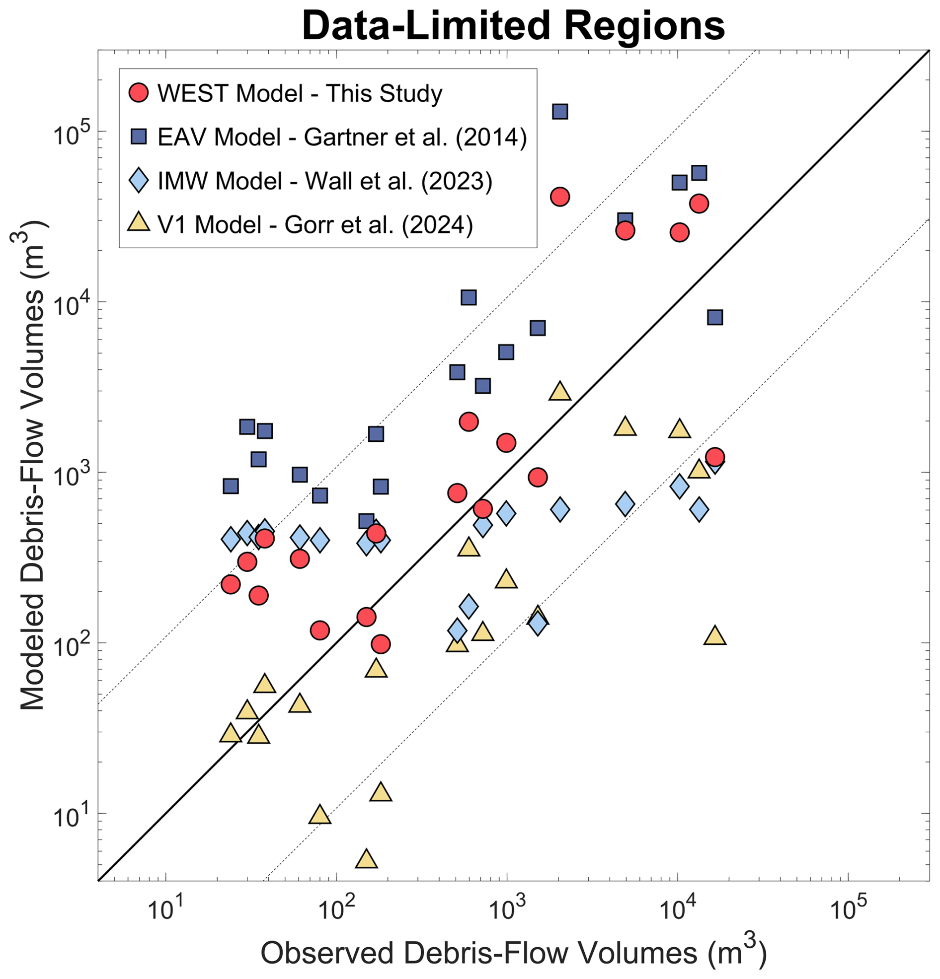
Figure 4 A comparison between the observed volume of 19 postfire debris flows from data-limited regions and the corresponding volume predicted by the western United States (WEST), Emergency Assessment volume (EAV), Intermountain West (IMW), and V1 models. The thick, black line is a 1:1 line, and the thin, dashed lines represent an order of magnitude envelope.

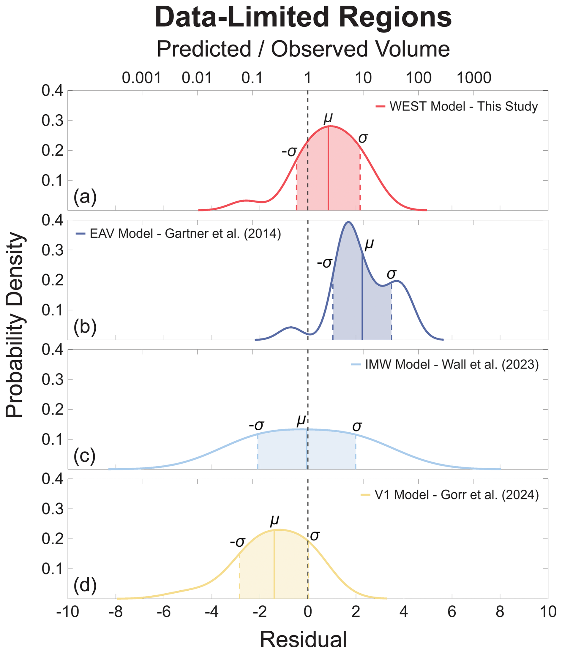
Figure 5 Probability density functions for the residuals of the (a) western United States (WEST), (b) Emergency Assessment volume (EAV), (c) Intermountain West (IMW), and (d) V1 models when applied to volumes from data-limited regions.

Regional volume models tend to be biased when applied outside of their training regions such that they overpredict volumes in areas with higher average rainfall intensities than their training region and underpredict volumes in areas with lower average rainfall intensities. For instance, southern California requires some of the least intense rainfall to generate postfire debris flows (Staley et al., 2017), so the EAV model (Gartner et al., 2014), which was developed using data from southern California (Gartner et al., 2014), tends to overpredict debris-flow volume in other regions of the western United States and Canada. Gorr et al. (2024a) found that the EAV model overpredicted postfire debris-flow volumes in the Southwest by roughly 3500 %, on average, and Rengers et al. (2024) found that the model overpredicted observed volumes in Colorado by more than a factor of four. Additionally, Gartner et al. (2024) found that the EAV model overpredicted postfire debris-flow volumes in British Columbia, Canada by a factor of 2 to 4. We observed similar model behavior in this study, as the EAV model consistently overpredicted postfire debris-flow volume in all regions other than southern California (Figs. 3, S4, and S5). Conversely, the Southwest requires some of the most intense rainfall to generate postfire debris flows (Staley et al., 2017), so the V1 model consistently underpredicts postfire debris-flow volumes in other parts of the western United States (Figs. 3, S3, and S4). In this study, the V1 model underestimated debris-flow volumes on all four subsets of data, as well as when applied to the entire western United States database (Fig. 3). It performed particularly poorly when applied to southern California (Fig. S3), the region with the least similar rainfall characteristics to the Southwest. The IMW model also consistently underpredicted postfire debris-flow volume in this study, including in the Intermountain West, the region for which it was developed (Fig. S4). However, this model does not include a rainfall variable (Wall et al., 2023), indicating that other regional differences or model limitations are responsible for reduced performance against this volume dataset.

The WEST model, however, does not exhibit large variations in model performance between geographic regions (Figs. S3–S5) because it uses i30 rainfall ratio instead of rainfall intensity (Eq. 2). This allows the WEST model to incorporate regional differences in rainfall intensity without the limitations associated with regional volume models. Because the i30 rainfall ratio normalizes the peak 30 min rainfall intensity of a debris-flow-producing storm by the peak 30 min rainfall intensity associated with a 1 year recurrence interval storm at the location of a debris-flow-producing watershed, it is consistent across regions that have different rainfall characteristics. As a result, the WEST model performs similarly when applied to different geographic regions, including southern California (Fig. S3), the Intermountain West (Fig. S4), and the Southwest (Fig. S5).

5.1.2 Training dataset

The WEST model also offers an improvement over existing postfire debris-flow volume models, as it was developed using a more comprehensive training dataset. The WEST model was developed using a dataset of 227 postfire debris-flow volumes from 34 burn areas across six states (Fig. 1). The 3 regional models evaluated in this study, on the other hand, were developed using smaller, more geographically limited datasets. Specifically, the EAV model was developed using 92 volumes from southern California (Gartner et al., 2014), the IMW model using 47 volumes from four states in the Intermountain West (Arizona, Colorado, Utah, and Wyoming), although 39 volumes were from Utah alone (Wall et al., 2023), and the V1 model using 54 volumes from Arizona and New Mexico (Gorr et al., 2024a). The geographic diversity of its training dataset contributes to the broader applicability of the WEST model relative to existing regional volume models.

The broad applicability of the WEST model indicates that it can be a substantial improvement over volume models that are currently used for postfire hazard assessments, including the EAV model. The EAV model is currently the most-commonly used method for predicting postfire debris-flow volume in the western United States, as it is used as part of the USGS operational postfire hazard assessment framework (Landslide Hazards Program, 2018). Although the accuracy of the EAV model is limited outside of southern California, as discussed above, a lack of postfire debris-flow volume data, and associated rainfall data, in many parts of the western United States has historically prevented the development of a viable alternative. When the EAV model was published in 2014, nearly all measured postfire debris-flow volumes with associated rainfall data were from southern California (Gartner et al., 2014), with minor exceptions from Arizona (Youberg, 2014), Colorado (Gartner et al., 2008), and Utah (Gartner et al., 2008). Taking the database used in this study (Gorr et al., 2025) as an example, more than 70 % of postfire debris-flow volumes measured prior to 2014 came from southern California (Fig. 6). The limited geographic scope of volume data available at the time therefore prevented the development of a more broadly applicable postfire debris-flow volume model.

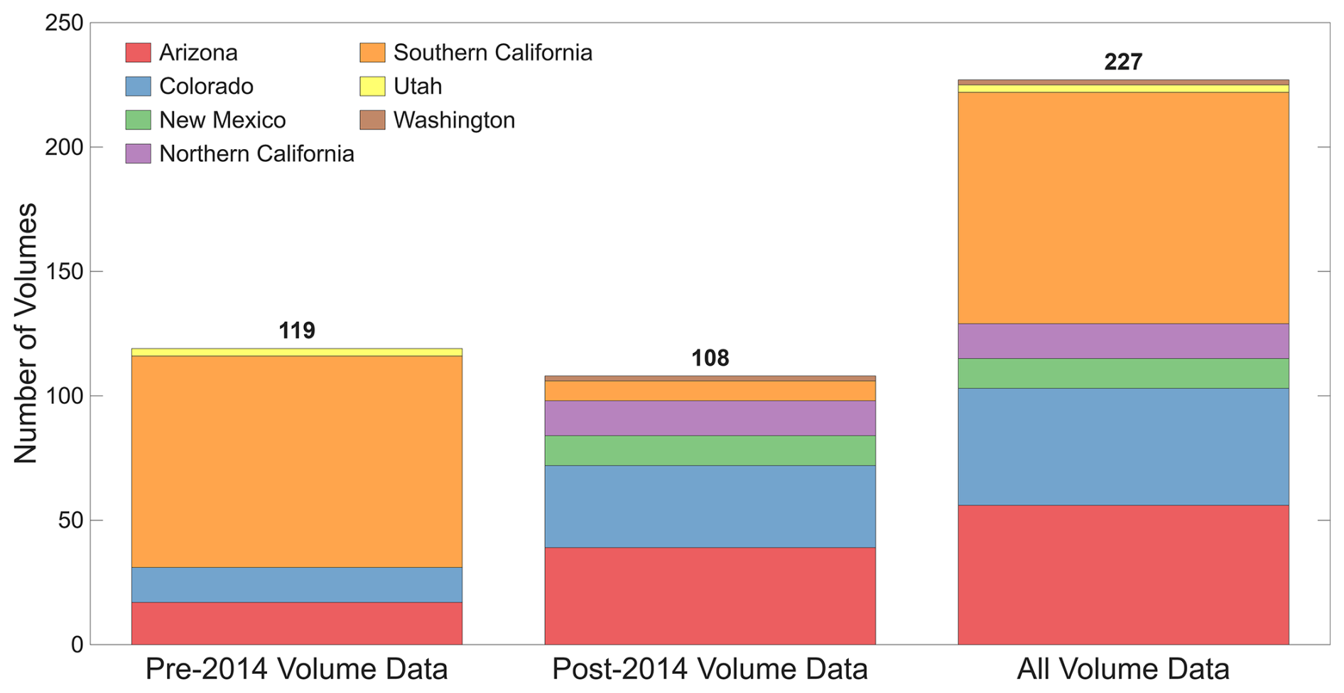
Figure 6 Geographic distributions of the volume data used to develop the western United States (WEST) model, separated by date of volume measurement. Specifically, the distributions of volume data collected prior to 2014, volume data collected after 2014, and all volume data included in the database used to develop the WEST model.

However, efforts to measure postfire debris-flow volumes across the western United States have expanded since the EAV model was published. Of the 227 postfire debris-flow volumes used to develop the WEST model, 108 (48 %) have been measured since 2014. Many of the volumes collected during this time are from regions where volume data have been historically sparse, and only 7 % of post-2014 volumes used in this study are from southern California (Fig. 6). All volumes from New Mexico, northern California, and Washington have been collected since 2014, and data from Arizona and Colorado have expanded by 229 % and 236 % relative to the pre-2014 dataset, respectively (Fig. 6). The improved performance of the WEST model across the western United States compared to existing models can therefore be partially attributed to the fact that it was trained on the largest and most geographically diverse postfire debris-flow volume dataset with associated rainfall data.

5.2 Implications for hazard assessment

Because it accounts for regional differences in rainfall characteristics and was trained on a geographically diverse volume dataset, the WEST model can be used for widespread postfire hazard assessments in the western United States. One of the most encouraging signs for improved postfire hazard assessments is the model's performance in data-limited regions. Results show that the WEST model performed similarly in data-limited regions as it did elsewhere in the western United States (Tables 5–8), and that it outperformed the EAV, IMW, and V1 models in these areas (Figs. 4 and 5). The WEST model performed particularly well, relative to existing models, against two debris-flow volumes from the Dixie Fire, which burned in the Sierra Nevada of northern California, and two volumes from the Cub Creek 2 Fire, which burned in the Pacific Northwest (Washington) (Fig. 1; Table 1).

The WEST model overpredicted the four volumes in the Sierra Nevada and Pacific Northwest by an average of 25 007 m³, which represents a substantial improvement over the EAV model, which overpredicted the same four volumes by an average of 59 284 m³. The IMW and V1 models, on the other hand, underpredicted these volumes by an average of 6981 and 5792 m³, respectively. Though the IMW and V1 models provided a smaller absolute difference between observed and modeled volumes in these regions, they severely underpredicted observed volumes in the Sierra Nevada and Pacific Northwest. Specifically, the IMW model underpredicted these four volumes by between 70.5 % and 95.5 %. The V1 model slightly overpredicted one of the four volumes by 41 % but underpredicted the remaining three by between 63.5 % and 92.4 %. Because previous studies have found that debris-flow volume scales with runout distance and area inundated (Iverson et al., 1998; Rickenmann, 1999; Griswold and Iverson, 2008), underpredicting debris-flow volume limits the effectiveness of postfire hazard assessments by underestimating the downstream effects of postfire debris flows. Based on the results of this study, the WEST model is less likely to underestimate the extent of potential downstream effects from postfire debris flows in data-limited regions, as it offers more conservative predictions of postfire debris-flow volume relative to the IMW and V1 models. At the same time, it provides more accurate volume estimates than the EAV model in these areas, making it less likely to predict unrealistically severe downstream effects.

Having a method that outperforms existing models in data-limited regions, such as the Sierra Nevada and Pacific Northwest, can improve postfire hazard assessments in these areas, particularly as fire activity increases. Wildfire activity across the western United States has increased considerably in recent decades, but this change has been particularly pronounced in the Pacific Northwest (Westerling, 2016). According to Westerling (2016), the area burned by wildfire in the Pacific Northwest between 2003 and 2012 increased by nearly 5000 % relative to the area burned in this region between 1973 and 1982. Furthermore, since this study was published in 2016, the Pacific Northwest has experienced multiple historic fire seasons, including the 2020 season, which burned nearly as much forest in the western Cascade Range in two weeks as in the previous five decades combined (Reilly et al., 2022). Fire activity is also increasing in California's Sierra Nevada (Westerling, 2016). Not only are fires in the Sierra Nevada increasing in size and frequency (Westerling, 2016), but the severity of fires is also changing. Miller and Safford (2012) found that proportion of annual wildfire burned at high severity increased considerably in parts of the Sierra Nevada between 1984 and 2010. This has important implications for postfire debris-flow hazards, as the effects of fire on infiltration and erosion, which affects debris-flow initiation and growth, are most pronounced in areas burned at high severity (e.g., Vieira et al., 2015; McGuire and Youberg, 2019). As fire activity in these regions increases, so does the potential for postfire debris-flow hazards (e.g., DeGraff et al., 2011; Neptune et al., 2021; Wall et al., 2020; Selander et al., 2025), underscoring the use of a volume model, like the WEST model, that can provide accurate estimates of debris-flow volume in these areas.

Additional volume data from the Sierra Nevada and Pacific Northwest will further improve predictions of postfire debris-flow volumes in these regions. However, this study represents a first step, as it is the first to include data from the Sierra Nevada and Pacific Northwest in the development and evaluation of volume models. In particular, volume data from larger-magnitude debris flows in data-limited regions are needed to more fully evaluate the performance of the WEST model in these settings, as the median volume of the 19 debris flows from data-limited regions included in this study was 511 m³ (Table S2), nearly five times lower than the median volume of 2550 m³ associated with the entire volume database. Additionally, volume data from the northern Rockies (Idaho, Montana, and Wyoming) are needed to evaluate the WEST model in this region. Although the northern Rockies are susceptible to postfire debris flows (e.g., Meyer and Wells, 1997; Gabet and Bookter, 2008), we are unaware of any postfire debris-flow volumes with associated rainfall data from this region that can be used to improve model performance.

Similarly, more data are needed to evaluate the performance of the WEST model when applied outside of the western United States. Although postfire debris flows are common hazards in fire-prone regions around the world, including Australia (e.g., Nyman et al., 2011), Canada (Hancock and Wlodarczyk, 2025), Italy (e.g., Esposito et al., 2023), and Spain (García-Ruiz et al., 2013), debris-flow volumes and associated rainfall data remain scarce outside of the western United States. This lack of data has limited the development of postfire debris-flow volume models for these regions and has prevented the evaluation of most volume models developed for use in the western United States, including the WEST model, when applied elsewhere. However, previous studies suggest that the primary controls on postfire debris-flow volume may be consistent across geographic regions. For example, Nyman et al. (2015) found that watershed area was the most important control on the volume of 10 postfire debris flows that initiated in southeast Australia and that volumes could be accurately predicted using an empirical volume model developed for use in the western United States (Gartner et al., 2008). Similar to the WEST model, this model predicts postfire debris-flow volume as a function of rainfall characteristics, watershed area and slope, and burn severity (Gartner et al., 2008). These similarities indicate that the primary controls on postfire debris-flow volume are generally transferrable across geographic settings, but additional volume data from fire-prone regions around the world are needed to evaluate the performance of the WEST model beyond the western United States.

Table 9 Equations for volume models that use rainfall ratios calculated at different durations, including 15 min (i15_rr), 30 min (i30_rr), and 60 min (i60_rr). All models predict debris-flow volume (V) as a function of rainfall ratio, watershed area (a), and watershed area burned at moderate or high severity with slopes ≥ 50 % (mh₅₀). Performance metrics include R² and root mean square error (RMSE), as well as the p-values for the Anderson–Darling (AD) and Brown–Forsythe (BF) tests.

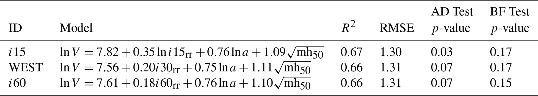
Finally, although we selected the WEST model using the criteria outlined in Sect. 3.2.2, several alternative models that we developed as part of this study offer similar performance metrics (Table S3) and may be preferred to the WEST model in some situations. For instance, we determined that rainfall ratio calculated over a 30 min duration yielded the best results for our dataset, but there may be scenarios where models that incorporate rainfall ratio calculated over 15 or 60 min durations are more suitable. It may be more practical, for example, to use a model that includes i60 rainfall ratio, instead of i30 rainfall ratio, to estimate volumes for a mitigation project if only i60 design storms are available. Alternatively, it may be easier to implement a model that uses i15 rainfall ratio within a hazard assessment framework that also predicts postfire debris-flow likelihood using rainfall characteristics measured over a 15 min duration (Landslide Hazards Program, 2018). Given their potential applicability in these scenarios, we present alternative models that use i15 and i60 rainfall ratio, along with the same terrain and fire variables used by the WEST model (Eq. 2), to predict postfire debris-flow volume in Table 9. Note that, although it marginally outperforms the WEST model, the i15 model does not pass the Anderson–Darling test (p-value < 0.05), so was not considered for final model selection. The i60 model, on the other hand, performs similarly to the WEST model and meets all requirements of multiple linear regression (Table 9).

5.3 Model limitations and future work

Although the WEST model improves our ability to predict postfire debris-flow volume in many regions of the western United States, there are some scenarios where the effectiveness of the model may be limited. For example, because the WEST model predicts postfire debris-flow volume as a function of both watershed area and watershed area burned at moderate or high severity with slopes greater than or equal to 50 %, it tends to substantially overpredict volumes from large watersheds (> 20 km²) (Fig. 7). We observed this model behavior when applied to the largest watershed in the dataset used in this study: Cucamonga Dam (Gorr et al., 2025). The Cucamonga Dam watershed, which burned in the 2003 Grand Prix Fire in southern California (Fig. 1), had an area of 28.0 km² and an area burned at moderate or high severity with slopes greater than or equal to 50 % of 14.8 km², both the largest in the volume dataset (Tables 3 and 4). It also produced the largest postfire debris flow in the dataset, with a volume of 801 770 m³ (Gorr et al., 2025). When applied to this watershed, the WEST model predicted a volume of 1 993 100 m³, an overprediction of more than 1 000 000 m³ (Fig. 7). However, we only expect this behavior in the watersheds larger than 20 km², like the Cucamonga Dam watershed, as the model slightly underpredicted the volumes for the next two largest watersheds in the dataset (Fig. 7), which had areas of 17.3 and 14.4 km². This limitation is unlikely to affect postfire hazard assessments in the western United States, as the USGS operational postfire hazard assessment framework is typically applied to watersheds with areas less than 8.0 km² (Landslide Hazards Program, 2018).

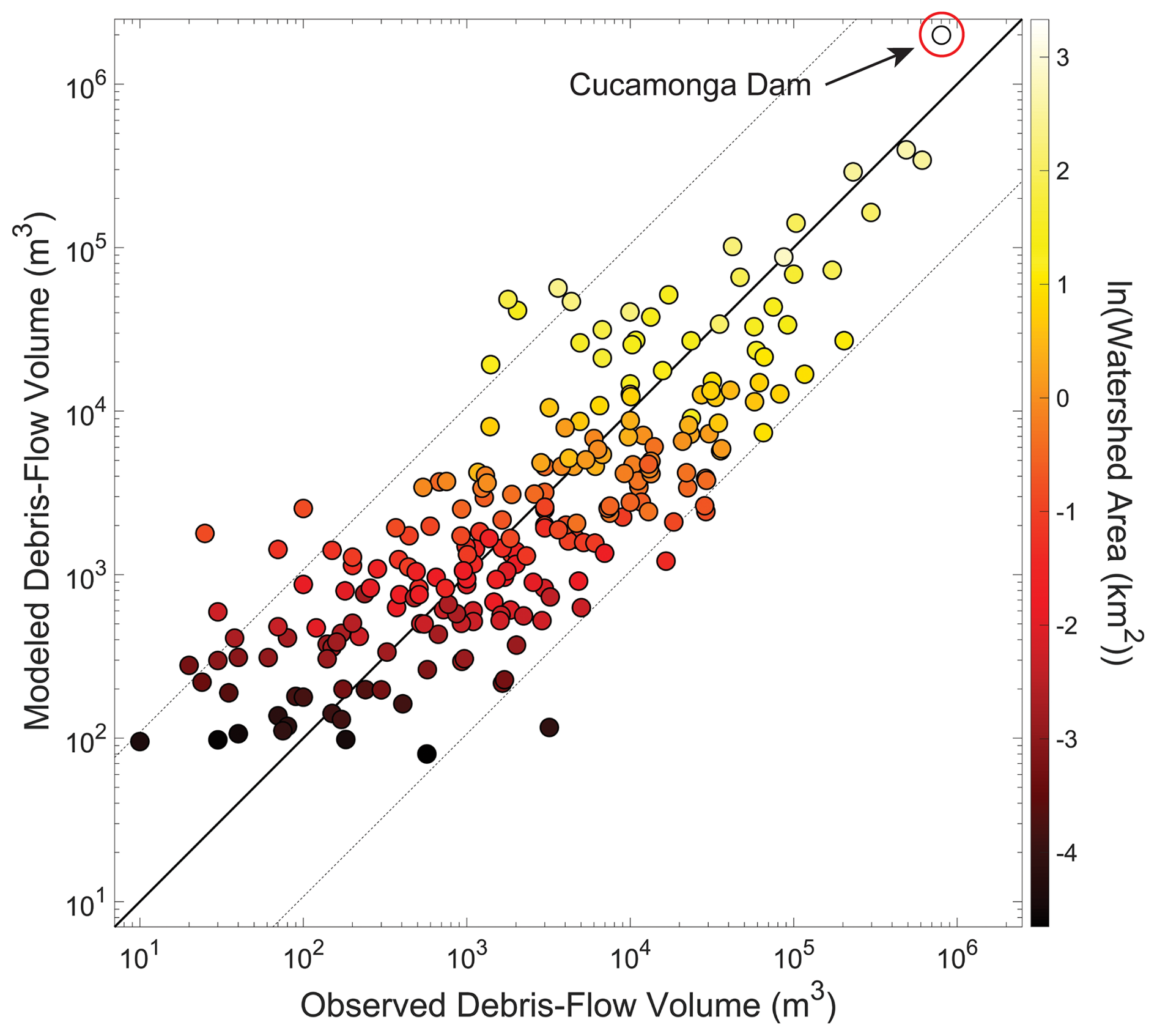
Figure 7 Comparison between observed debris-flow volumes and debris-flow volumes predicted by the Western United States (WEST) model when applied to the entire western United States dataset. Points are colored by the natural log of the area of the debris-flow-producing watershed. The thick, black line is a 1:1 line, and the thin, dashed lines represent an order of magnitude envelope.

Another potential limitation of the WEST model is that, aside from differences in rainfall characteristics, it does not account for other regional factors that may influence postfire debris-flow volume, including sediment availability. In southern California, dry ravel (i.e., the transport of sediment by gravity without rainfall) is a common process in burned landscapes (e.g., Lamb et al., 2011). Following fire, but before rainfall, dry ravel can load channels with up to 3 m of unconsolidated sediment that serves as an important sediment source for postfire debris flows (e.g., Wells II, 1987; DiBiase and Lamb, 2020; Palucis et al., 2021). Although prevalent in southern California, dry ravel is less common in other regions of the western United States (Perkins et al., 2022). Previous studies have found that rilling on hillslopes and/or channel incision, not dry ravel, are the primary sources of sediment for postfire debris flows in many areas, including elsewhere in California (e.g., DeGraff et al., 2011), Colorado (Rengers et al., 2024), the Pacific Northwest (Wall et al., 2020), and the Southwest (e.g., Tillery and Rengers, 2020; Gorr et al., 2024b), among others. The absence of dry ravel in these regions may limit sediment availability and result in smaller postfire debris-flow volumes relative to southern California. Regional differences in sediment availability may account for differences in model behavior that we observed in this study. In areas with dry ravel (i.e., southern California), the WEST model is biased low (Fig. S3), and in areas where dry ravel is less prevalent (i.e., the Intermountain West and Southwest), the WEST model is biased high (Figs. S4 and S5). This indicates that future postfire debris-flow volume models may benefit from the inclusion of a sediment availability variable.

6 Conclusions

Debris-flow volume is a critical component of postfire hazard assessments in the western United States. However, existing methods for predicting postfire debris-flow volume have various shortcomings that limit their applicability for the purpose of postfire hazard assessment. In this study, we introduced a new model for predicting postfire debris-flow volume in the western United States. Using a database of 227 postfire debris-flow volumes collected across six states and 34 burn areas, we developed a multiple linear regression model that predicts postfire debris-flow volume as a function of rainfall, watershed terrain, and fire characteristics. This model offers an improvement over existing volume models, as it accounts for regional differences in debris-flow-generating rainfall and was trained on a larger, more geographically diverse volume dataset. Results from this study demonstrate that the new model outperforms 3 existing regional volume models when applied to the entire western United States database, and either outperforms or performs similarly to existing regional volume models when applied to subsets of volume data from the regions for which they were developed. The new model also outperforms existing models when applied to volumes from data-limited regions where there is not enough data to develop region-specific models. The broad applicability of the model introduced in this study indicates that it can be used to improve widespread postfire hazard assessments across the western United States.