Leveraging reforecasts for flood estimation with long continuous simulation: a proof-of-concept study

Flood estimation is critical for risk assessment, but traditional approaches are often constrained by the limited length of observational records. This study explores the potential of reforecasts (RFs) for flood estimation using long continuous simulation (CS) with a hydrological model at high (hourly) temporal resolution. As a proof of concept, we first processed individual RFs from the extensive archive of the European Centre for Medium-Range Weather Forecasts (ECMWF) with bias correction, stochastic downscaling and disaggregation with analogs to obtain mean areal precipitation and mean areal temperature for a set of test catchments in Switzerland. We subsequently concatenated these RFs into a time series of nearly 10 000 years and used them in long CS to derive flood return levels.

Results show hydrological consistency of the concatenated RFs and demonstrate their potential in flood estimation, providing information on the magnitude and frequency of extreme events. In addition, RFs offer a relevant complementary perspective on exceptionally large floods when compared with estimates derived from long CS driven by other forcing inputs, such as a stochastic weather generator. However, structural uncertainties – particularly related to the underlying numerical weather prediction system – must be considered, along with the reliance on a single model framework, non-stationarity and internal climate variability. Further limitations arise for catchments smaller than approximately 500 km², for which stochastic downscaling becomes increasingly inadequate. For resolving the relevant convective events in such catchments, dynamical downscaling would be more appropriate; however, this was not feasible with the currently available data.

1 Introduction

Rare to very rare floods, associated with return periods of 1000–10 000 years, can cause severe human and economic damage. However, their estimation is constrained by the comparatively short length of available streamflow records and by uncertainty about whether disaster-rich and disaster-poor periods within these records are representative of present conditions (Redmond et al., 2010; Schmocker-Fackel and Naef, 2010a, b; Zeder and Fischer, 2024). At the upper end of the flood magnitude spectrum, the estimation of very rare or unprecedented floods – and of weather hazards more generally (see Kelder et al., 2025) – is addressed using a variety of approaches. These include converting estimates of probable maximum precipitation (PMP) into probable maximum floods (PMF) (World Meteorological Organization, 2009), applying weather generators in hydrological simulations (Lamb et al., 2016), pooling large regional data sets of observed floods (Bertola et al., 2023), and developing storylines based on extremely rare observed events (e.g., de Bruijn et al., 2023).

With respect to meteorological extremes more broadly, reforecasts (RF) have been used to explore plausible yet unobserved extremes that are difficult to infer from historical records alone. Although the primary purpose of RFs is forecast skill assessment and calibration (Robertson and Vitart, 2019), the extensive archive of model realisations under current atmospheric conditions provided by ensemble prediction systems (Kelder et al., 2022) offers an opportunity to explore meteorologically plausible extreme events beyond the observed range. RFs are typically initialised from observed atmospheric states but simulate conditions beyond the predictability horizon, diverging from the observed meteorological evolution. Consequently, RFs represent plausible, yet unrealized, atmospheric evolutions, including extreme events that have not been observed to date (Thompson et al., 2017).

RFs have been applied to estimate extreme sea surges (van den Brink et al., 2004), precipitation (Thompson et al., 2017; Kelder et al., 2020), temperature (Thompson et al., 2019; Kay et al., 2020) and wind (Osinski et al., 2016), as well as to characterize compound events (Hillier and Dixon, 2020). In relation to estimation of extreme floods, Brunner and Slater (2022) pooled RF ensemble members of river discharge from the European Flood Awareness System (EFAS) to examine the frequency and intensity of extreme floods, with return periods of up to 200 years across Central European catchments. Compared to flood estimates derived from observations, this approach yielded considerably narrower uncertainty bounds for extreme events occurring less than twice a century. Similarly, Klehmet et al. (2024) investigated the robustness of frequency estimates for daily precipitation and streamflow extremes with return periods of up to 500 years using synthetic time series derived from pooled SEAS5 seasonal RFs (Johnson et al., 2019). These series were used to generate hydrological RFs with the process-based E-HYPE model (Hundecha et al., 2016) across Europe. By generating 100 samples with replacement for different time-series lengths, they showed that the relative interquartile range of estimated 100-year return levels – a measure of sampling uncertainty – decreased markedly with longer time series, from above 100 % for 50-year time series to below 10 % for 500-year series. Building on these approaches, Ganapathy et al. (2024) introduced an additional step to account for different flood type clusters by applying a mixing distribution after pooling. Using RF data from the Global Flood Awareness System (GLOFAS) and the UNprecedented Simulated Extreme ENsemble (UNSEEN) method (Kelder et al., 2020, 2022), they analysed two catchments in Germany with return periods of up to 200 years. Their results indicate that explicitly representing flood types alters the estimated 100-year return level by at least 15 % and reduces the Root Mean Square Error (RMSE) compared with conventional single-distribution approaches. Applications of the UNSEEN framework using RFs therefore extend beyond flood frequency estimation and also support the construction of plausible unprecedented-event storylines under varying initial conditions (Kay et al., 2024).

Here, we examine the feasibility and added value of using extensive RF precipitation and temperature data within an established long continuous simulation (CS) framework at hourly resolution. This framework avoids assumptions about antecedent conditions and their spatial patterns while enabling a physically coherent representation of the full spatio-temporal evolution of floods over larger areas (Lamb et al., 2016). To ensure comparability with an existing long CS framework that relies on weather generator (WGEN) input, we adopted the hydrometeorological simulation chain introduced by Viviroli et al. (2022), which forms the foundation for the EXAR (hazard information for extreme flood events on the rivers Aare and Rhine) (Andres et al., 2021) and EXCH (Extreme Floods in Switzerland) (Viviroli et al., 2025) projects. Both initiatives aim to deliver methodologically and spatially consistent flood hazard assessments, evaluated as comprehensively as possible given the limited information available on rare events.

For consistency and comparability with the EXAR/EXCH framework, several methodological choices were retained, including the use of a lumped catchment model with hydrological routing where required and the interpolation of mean catchment meteorological inputs from point values. Although specific elements of this procedure could be refined, the adopted framework enables direct juxtaposition of RF-based flood estimates, derived from physically consistent and plausible weather conditions, and WGEN-based estimates generated within a stochastic multi-site framework. This juxtaposition provides valuable context for assessing very rare floods.

Against this background, this study is designed as a proof of concept to address the following research questions:

1. Can raw RF data be processed to hourly resolution and concatenated into very long time series suitable for continuous hydrological simulation in a challenging Alpine setting?

2. How do flood frequency estimates derived from such RF-based continuous simulations compare with, and complement, estimates obtained using an established stochastic weather generator framework?

3. What are the key limitations of the RF-based approach within a long CS framework?

To address these questions, we processed RFs from the European Centre for Medium-Range Weather Forecasts (ECMWF) using bias correction, stochastic downscaling, and temporal disaggregation, and concatenated the RFs into a 10 000-year time series. These series were then used as input for hydrological simulations, which were compared with simulations driven by a stochastic weather generator to evaluate feasibility, added value and limitations of the RF-based approach.

2 Data

2.1 Test catchments

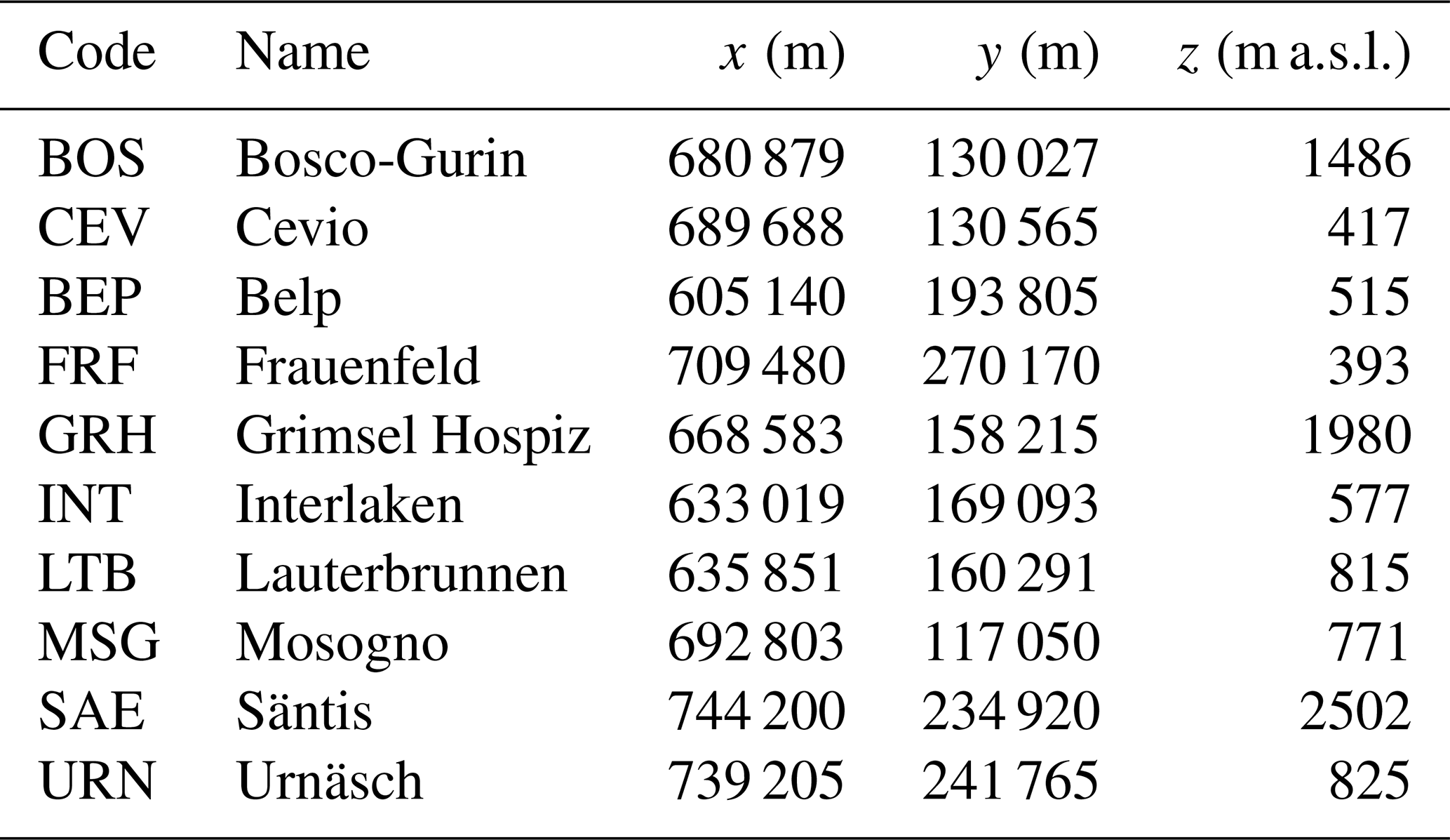
For our proof of concept, we examined a total of 20 test catchments (Table 1 and Fig. 1) from across Switzerland. These catchments represent important climate regions and runoff regime characteristic of a region with complex topography. Note that three catchments in each of the Aare river basin (Kander at Hondrich, Aare at Thun, Aare at Bern), the Thur river basin (Thur at Alt St. Johann, Thur at Jonschwil, Thur at Andelfingen) and the Maggia river basin (Riale di Calneggia at Cavergno, Isorno at Mosogno, Maggia at Locarno) are nested. The sites on the Aare, Drance de Bagnes, Maggia, Saltina and Sarine rivers are impacted by hydropower, and the Thun and Bern sites on the Aare River are influenced by the regulated lakes Brienz and Thun.

Table 1 Test catchments examined in this proof-of-concept study, with area (A), mean catchment elevation (E) and runoff regime type (Weingartner and Aschwanden, 1992). The catchments are grouped by climate region (Bundesamt für Umwelt BAFU, 2022) and listed in order of decreasing area.

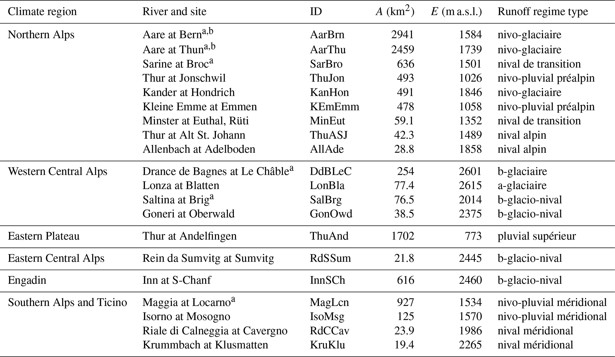
^a Flows at these sites are impacted by hydropower operations (see Margot et al., 1992).
^b Flows at these sites are impacted by regulated natural lakes.

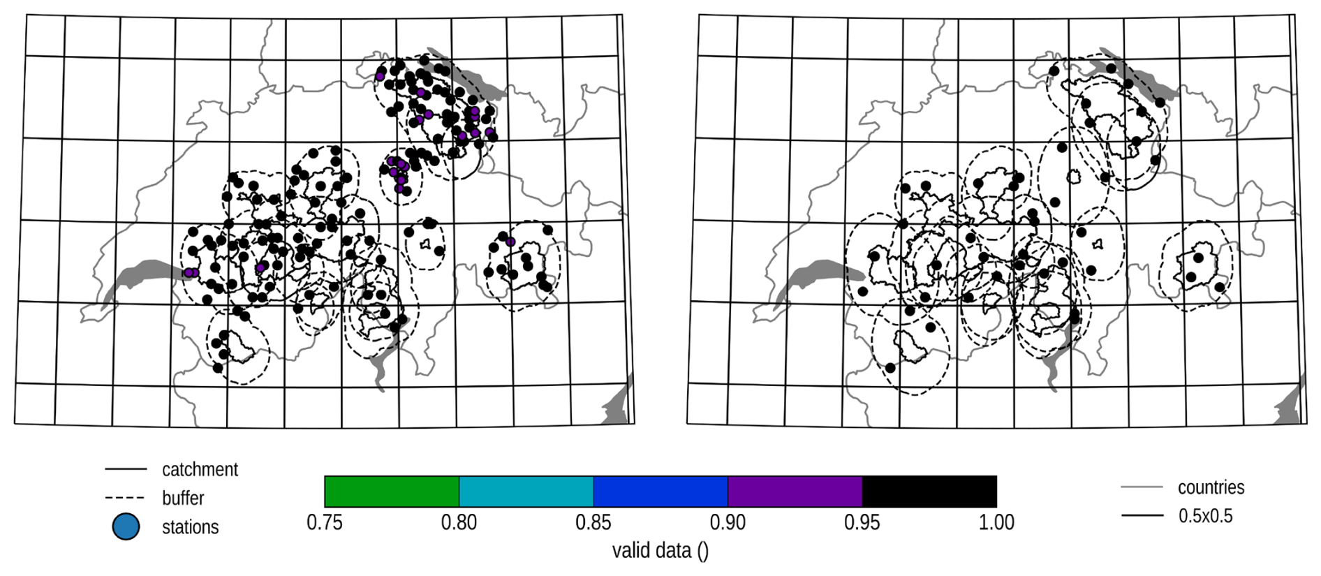
Figure 1 Study region with catchments (solid black lines) and meteorological stations (dots), also showing temporal coverage of station data for precipitation 1961–2019 (left) and temperature 1991–2019 (right). The 0.5° grid ($\sim \mathrm{38}\times \mathrm{56}{\mathrm{km}}^{\mathrm{2}}$) shown is equivalent to that of the reforecasts used. Dashed black lines indicate the buffer zone around the catchment used in the statistical downscaling.

2.2 Reforecast data

Our work is based on the ensemble RFs provided by the ECMWF Integrated Forecasting System (IFS) that allows considering plausible yet not actually occurred weather extremes (Owens and Hewson, 2018). For the statistical modelling, we used precipitation and near-surface air temperature as input. The data were available on a 0.25° regular grid ($\sim \mathrm{19}\times \mathrm{28}{\mathrm{km}}^{\mathrm{2}}$ in the study domain) until forecast day 15, and on a 0.5° regular grid ($\sim \mathrm{38}\times \mathrm{56}{\mathrm{km}}^{\mathrm{2}}$) thereafter. The temporal resolution of the data was 6 h.

ECMWF's IFS has undergone several changes since its inception in 2008 (ECMWF, 2024a, b, 2025). As detailed in Table 2, the ECMWF RFs (control and perturbed)

• are initialised weekly March 2008–May 2015, and bi-weekly from May 2015 onwards,

• are initialised for the leading 18 years March 2008–June 2012, and for the leading 20 years from June 2012 onwards,

• provide 4 ensemble members from March 2008–May 2015, and 10 ensemble members from May 2015 onwards, and

• provide forecasts for a period covering 31 d (March 2008–May 2015), and 46 d from May 2015 onwards.

In addition, the IFS underwent regular updates over the years, often multiple times per year (Table 2). To benefit from as much data as possible and derive a large collection of yearly time series for hydrological modelling, data from the different IFS cycles initialised within the same year were treated uniformly.

However, a visual examination of the RF precipitation and temperature by forecast lead time and by initialisation year revealed two systematic inconsistencies (Fig. S1 in the Supplement):

1. The precipitation data show a spike on the transition day between medium-range ensemble (ENS) RFs (days 1–15) and the extended range RFs (days 16–46).

2. The temperature data for RFs initialised in 2015 have a strong drift over the forecast period.

To address the first issue, we discarded the first 15 d and used only data from day 16 onward, corresponding to the extended range RFs. This also ensures a high degree of independence among individual ensemble members, as discarding the first 10 d alone would have been sufficient for our application domain (Mahlstein et al., 2019). To resolve the second issue, we discarded the year 2015 entirely. We also excluded the year 2008, as it does not provide a full year of data. Residual inhomogeneities arising from the evolution of the IFS model across the archive period were further addressed in the bias adjustment (Sect. 3.2.1) and concatenation steps (Sect. 3.2.4). As a result, data with a total length of more than 10 000 years were available for analysis and processing.

Table 2 Reforecasts by initialisation year, showing number of initialisation per week, number of years reforecasted, number of members, the available forecast length (from day 16 onwards) and the respective IFS cycles for each year (ECMWF, 2024a, b, 2025). Note that years 2008 and 2015 were not used in this study.

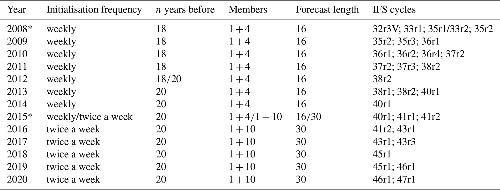
* Not used in this study.

2.3 Meteorological data

We employed a statistical model to relate the gridded RF data to the point scale. As a meteorological reference for grid-scale precipitation, we used RhiresD, a spatial precipitation analysis provided by MeteoSwiss (2021a), which provides daily precipitation data from 1961 onwards at a 1 km raster resolution. Additionally, we evaluated the hourly MeteoSwiss product CombiPrecip (Sideris et al., 2014), which combines weather radar fields with point precipitation measurements from 2005 onward, also at a 1 km resolution. However, CombiPrecip was used only for disaggregating daily precipitation (Sect. 3.2.3) because the data, despite MeteoSwiss' elaborate processing (Germann et al., 2022), are noticeably affected by terrain shielding of the radar beam. Moreover, CombiPrecip data are only available from 2005 onward, which is too short for robust bias adjustment. We also examined two further gridded observation products but discarded them due to their limitations in the present context: E-OBS (Cornes et al., 2018), which has a comparatively low station density; and WFDE5 (Cucchi et al., 2020), which matches the grid point resolution of the coarse RFs (0.5°) but is offset by half a grid point.

As a meteorological reference for grid-scale temperature, we considered a spatial analysis of mean, minimum and maximum temperature provided by MeteoSwiss (2021b), which provides daily data from 1961 onwards at a 1 km raster resolution. However, we instead directly bias-adjusted RF temperature data against station observations and did not use this gridded analysis. Unlike precipitation, which exhibits strong stochastic sub-grid variability that direct quantile mapping cannot reproduce without introducing artefacts (Maraun, 2013; Maraun et al., 2017), temperature varies smoothly in space, making station-based bias adjustment appropriate.

As a meteorological reference at the point scale for both precipitation and temperature, we used station data obtained from MeteoSwiss (2025, retrieved 1 May 2021). The temporal and spatial coverage varied between the available daily and the hourly gauging networks, and for consistency with the approach used in the projects EXAR/EXCH, we used hourly station observations aggregated to the daily scale for both the stochastic downscaling of precipitation and the quantile mapping of temperature (see Sect. 3.2).

2.4 Hydrological data

The continuous hydrological data encompassed hourly discharge records for the test catchments listed in Table 1. These data were available for a maximum period from 1974–2021. However, most time series were shorter, with a median length of 30 years and a range of 6–47 years. In addition, records of annual maximum floods (AMFs) were available for most of these stations. These records refer to instantaneous peak flow and date back even further, with a median length of 63 years and a range of 23–118 years. Extrapolations of the observed AMFs via the generalized extreme value (GEV) distribution were also available for these stations (Baumgartner et al., 2013). Maximum flood data from all over Switzerland were available from Kienzler and Scherrer (2018), covering measurements and historical reconstructions at 740 sites in total.

2.5 Hydrometeorological scenarios based on weather generator

For comparison, 300 000 years of hourly simulation results from a hydrometeorological model chain using the Generator of Weather EXtremes (GWEX) WGEN were available. GWEX is a multi-site, two-part stochastic weather generator for precipitation and temperature, based on the structure proposed by Wilks (1998). It is designed to reproduce the statistical behaviour of weather events at various temporal and spatial resolutions, with a focus on extremes. Since comparatively long events are relevant in the main EXAR/EXCH framework, GWEX first generates 3 d precipitation amounts. These amounts are then disaggregated into daily and ultimately hourly values using meteorological analogs. Details on GWEX are found in Evin et al. (2018, 2019), while its application to flood estimation is discussed in Viviroli et al. (2022, 2025).

3 Methods

3.1 Experimental design

The methodology was designed to address the research questions outlined in the Introduction by processing ECMWF RF data into spatially coherent hourly series, concatenating these into multi-millennial continuous sequences and evaluating their suitability for long continuous hydrological simulations to estimate flood frequency at the catchment scale.

The workflow starts with bias adjustment of RF precipitation and temperature data, stochastic downscaling to multiple meteorological stations, disaggregation to hourly resolution and concatenation into long series (Sect. 3.2). Mean catchment values were then derived via interpolation and adjusted to mean catchment elevation (Sect. 3.3). The hydrological simulations employed a lumped catchment model with hydrological routing where necessary. As noted in the Introduction, we retained the main components and methodological choices of an established long CS framework (Andres et al., 2021; Viviroli et al., 2022) to enable direct comparison with simulations based on a stochastic weather generator. The only modification in the present study is that the meteorological forcing is derived from RFs rather than from a stochastic weather generator.

3.2 Statistical postprocessing of reforecasts

Statistical postprocessing was applied to transform the coarse-resolution RF data into spatially coherent, hourly time series of precipitation and temperature in Alpine catchment conditions, while preserving extreme events beyond the observed record (Fig. 2). All steps were applied to each test catchment (Sect. 2.1).

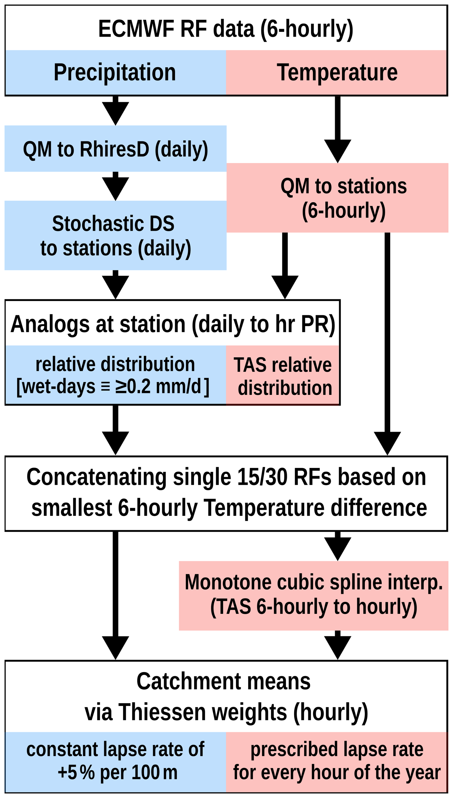
Figure 2 Workflow of statistical postprocessing, beginning with ECMWF raw reforecast (RF) data and proceeding through bias adjustment and stochastic downscaling (DS), application of analogs, concatenation, and interpolation to mean catchment values. PR is precipitation, TAS is temperature.

As a model-derived product, the RF data are subject to biases, particularly at longer lead times, and they are available at coarse spatial and temporal resolution. The postprocessing therefore comprised three components: bias adjustment, downscaling to station locations, and temporal disaggregation.

For precipitation, we followed the conceptual approach by Volosciuk et al. (2017) and first bias-adjusted the gridded RF precipitation data at their native resolution using quantile mapping against the gridded observations of RhiresD (Sect. 3.2.1). This separation of bias adjustment and downscaling avoids artefacts associated with direct calibration to station data (Maraun et al., 2017). The adjusted precipitation data were subsequently downscaled to multiple locations using a multi-site stochastic downscaling model based on a truncated and transformed multivariate Gaussian distribution (Switanek et al., 2022), preserving spatial coherence among stations (Sect. 3.2.2). Daily precipitation totals were then disaggregated to hourly resolution using analogs (see Sect. 3.2.3).

Two-meter air temperature (TAS) was bias adjusted directly to the station locations using daily data, with correction factors applied to the 6-hourly RF data. After concatenating single 15/30 d long RFs, hourly series were built using cubic spline interpolation. Finally, mean catchment precipitation and temperature were derived by Thiessen interpolation, using a constant adjustment factor for precipitation and a prescribed lapse rate for temperature following Viviroli et al. (2022).

3.2.1 Bias adjustment

In a first step, the RFs were bias-corrected separately for each month via basic quantile mapping (QM) (Jakob Themeßl et al., 2011), a common state-of-the-art bias adjustment method. For precipitation, we used RhiresD as a reference, with daily data from the period 1991–2020. For temperature, we used station data located within a ∼10–20 km buffer zone around the catchment as a reference, with data from the period 1991–2020. Temperature was bias corrected using daily data, and applying the correction value to the 6-hourly data. Since the bias structure for temperature and precipitation in the RFs varied by year of initialisation (see Sect. 2.2), the periods 2009–2014 and 2016–2020 were adjusted separately (excluding 2015, which was discarded, see Sect. 2.2).

A key objective was to retain the expected upper tail of the RF precipitation distribution, as the added value of RFs for flood estimation lies precisely in their ability to sample extremes beyond those observed. Since direct bias correction would eliminate such heavy precipitation events, a transfer function was applied: the RF distribution was estimated using non-overlapping samples of the same length as the observational data, and corrections were applied based on quantile differences between observations and the RF sample mean (Fig. 3).

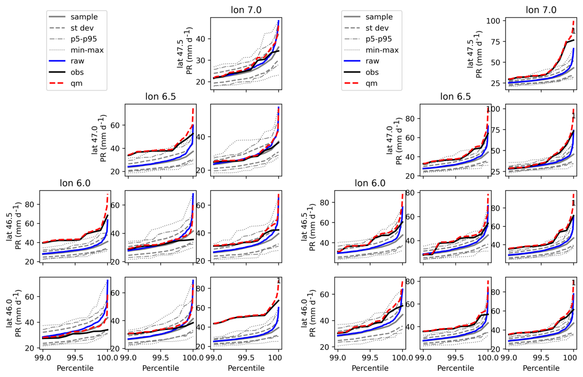
Figure 3 Daily precipitation (mm d⁻¹) above the 99th percentile for January (left) and August (right). Shown are RhiresD (“obs”, dashed black line), ECMWF raw reforecast data (“raw”, blue line), bias adjusted reforecast data (“qm”, red dashed line), and the transfer function on which the correction is based (“sample”, gray solid line) for selected grid points over Switzerland.

3.2.2 Stochastic downscaling

The downscaling ensures that small-scale spatial variability characteristic of Alpine precipitation is represented consistently across multiple stations, which is essential for realistic flood simulations at the catchment scale. We used a stochastic downscaling approach and adapted code of Switanek et al. (2022) to handle missing station data.

We applied this stochastic downscaling for each month and for each test catchment individually, using RhiresD and daily station data for calibration over the period 1961–2019. Stations with more than 25 % missing data during this period were excluded. Calibration with 6-hourly instead of daily station data produced unrealistic values for some sites and was therefore discarded. In addition to stations within each catchment, we included all stations located within a ∼10 km buffer zone around the catchment.

We adjusted the simulated data for mean bias but omitted the quantile-based multiplicative bias adjustment because it led to poorer performance in a split-sample test (see Switanek et al., 2022). We also tested the impact of extending the range of predictor grid points, but found no discernible difference between including grid points up to 0.75° or 1.25° from the nearest stations. We therefore used grid points within 0.75° for the final downscaling.

3.2.3 Analogs and disaggregation

Sub-daily precipitation dynamics are decisive for flood peaks in Alpine catchments. Therefore, realistic hourly disaggregation is critical for evaluating the suitability of RFs for flood frequency estimation. The bias-corrected and downscaled daily precipitation data were therefore disaggregated to the hourly resolution required for hydrological modelling. We applied the analog method because it is relatively straightforward to implement and generally produces spatially and temporally coherent results. To provide a large pool of reference data to draw the analogs from, we used daily and hourly station data (point measurements) as well as hourly CombiPrecip data (1×1 km² raster).

First, stations within each catchment and its vicinity were selected. Then, for each station, days with both daily and hourly data available during 1981–2019 were identified. For days with only daily station data, disaggregation was based on daily fractions derived from hourly CombiPrecip data for the period 2005–2019. Analogs were drawn separately for each month using a moving window of ±1 month. Further, the data were separated into dry and wet days using a threshold of 0.2 mm d⁻¹ for daily catchment precipitation interpolated with Thiessen weights. For dry days ($<\mathrm{0.2}\mathrm{mm}{\mathrm{d}}^{-\mathrm{1}}$), hourly precipitation was set to zero. For wet days, daily precipitation totals were disaggregated to hourly values using relative hourly contributions of the selected analogs at the station scale. All days within ±1 month of the modelled day were used. The best analog day was identified by computing the RMSE of precipitation and mean daily temperature at the station locations for all candidate days and selecting the day with the smallest combined RMSE.

3.2.4 Concatenation

To enable long continuous simulation, the short (15 or 30 d, depending on the initialisation year) RF segments were concatenated into synthetic annual sequences while minimizing artificial discontinuities at the stitching points. For consistency across years, a length of 360 d was assumed, consisting of 24 or 12 single RFs, respectively. RF segments were drawn exclusively from the same initialisation year to avoid mixing different IFS cycles, which could introduce inconsistencies (cf. Sect. 2.2).

To approximate the annual cycle, RFs were selected such that their initialisation dates collectively span one calendar year. For instance, for forecasts before 2015 (initialised weekly with a length of 15 d), synthetic years were constructed using every second initialisation week, resulting in two sets of years with identical initialisation dates. Because the 15 d forecast length differs from the 14 d interval between initialisation dates, a small temporal offset accumulated over the year. This was addressed by discarding single initialisation dates. This procedure yielded a total of 9920 synthetic 360 d years.

The selection of individual RFs used to construct a year was based on minimizing temperature difference at the stitching points at the catchment scale. Raw 6-hourly temperature data were used to evaluate differences at the same time step. Grid points were weighted according to station locations and their Thiessen weights. At the beginning of the assembly for a given initialisation year, subsequent RFs can be drawn from a large pool of reforecast-year ensemble members, allowing selection of RF segments with minimal temperature discontinuities. As more years are constructed, the pool decreases, leading to larger temperature differences between consecutive RF segments. Mean differences across all date combinations remained well below 1 °C for about three quarters of the ensemble-member selection steps and increased to about 5 °C for the final year assembled in the sequence. The mean overall maximum temperature differences across individual years and selection steps increased from approximately 0.1 °C to about 14 °C for the last assembled year. In the final hourly time series, derived from 6-hourly station temperature data using monotone cubic spline interpolation, these differences were around one sixth of those values. A detailed view of the temperature differences at the stitching points is provided in Fig. S2, and Fig. S3 illustrates a year with a pronounced temperature jump. The influence of these stitching artefacts on simulated AMFs is evaluated in Sect. 4.2.

3.3 Continuous hydrological simulation and routing

The following hydrological modelling framework was used to evaluate whether RF-based meteorological inputs produce internally consistent discharge simulations suitable for flood frequency analysis within a long CS approach. The complete concatenated RF precipitation and temperature data were finally used as input for the bucket-type catchment model HBV (Hydrologiska Byråns Vattenbalansavdelning model, see Seibert and Vis, 2012). HBV was calibrated on hourly data spanning 1983–2019, and run at an hourly time step, employing the non-linear response function of Lindström et al. (1997) to better represent flood behaviour (see Kritidou et al., 2026). To achieve mean areal precipitation and mean areal temperature time series required for hydrological modelling in the given long CS framework, the RF values downscaled to meteorological station locations were interpolated using Thiessen polygons. Precipitation was adjusted for differences between the Thiessen-weighted mean station elevation and the mean catchment elevation, applying a constant factor with a linear increase of 5 % for every 100 m (see e.g., Farinotti et al., 2012; Ménégoz et al., 2020; Ruelland, 2020; Viviroli et al., 2022). For temperature, calendar-based lapse rates were estimated from 1981–2019 data for each hour and each day of the year, differentiated for six large river basins (see Viviroli et al., 2025).

Observed precipitation and temperature data from 1931–2019 were interpolated similarly to mean areal values and used for a control run with HBV.

In catchments strongly affected by hydropower operations, lake retention, lake regulation, bank overflow or floodplain retention, hydrological routing was applied using RS Minerve (García Hernández et al., 2020) to account for these effects.

Further details on the hydrological simulation set-up are provided in Viviroli et al. (2022).

4 Results

4.1 Stochastic downscaling

Figure 4 shows simulated and observed mean daily catchment precipitation (left) and mean wet day frequency (right). Note that there is a mismatch between the station observations used in processing the RFs and the data shown at the point scale: The station observations are based on all available observed days over 1991–2019, which roughly coincides with the period used for the quantile mapping (1991–2020), while the stochastic downscaling was calibrated using grid data and station observations over the period 1961–2019. The stochastic downscaling reproduced these mean characteristics well. Figure 5 shows simulations and observations at single station locations (circles) and in the Thiessen weighted mean (crosses) for the catchment of the Aare River at Bern. Also for the single stations, the mean characteristics are reproduced well. There is a tendency for a small underestimation of mean precipitation for single stations and months, and some deviations from observed wet-day frequency, which might be explained by the different data periods used for the bias adjustment and for calibrating the stochastic downscaling, as well as associated sampling differences of large-scale modes of variability such as the Atlantic Multidecadal Oscillation (AMO) (see also Sect. 5.4).

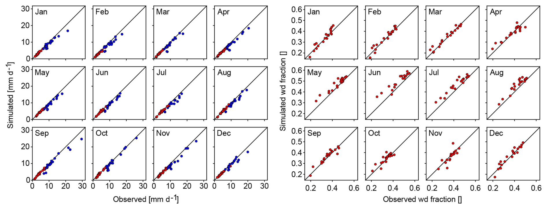
Figure 4 Left: Mean simulated and observed daily precipitation per month over all catchments for all day mean (red circles) and wet day mean ($>\mathrm{1.0}\mathrm{mm}{\mathrm{d}}^{-\mathrm{1}}$, blue circles). Right: Mean simulated and observed wet day frequency per month (expressed as fraction of days per month) over all catchments (red circles). Station observations are for the period 1991–2019.

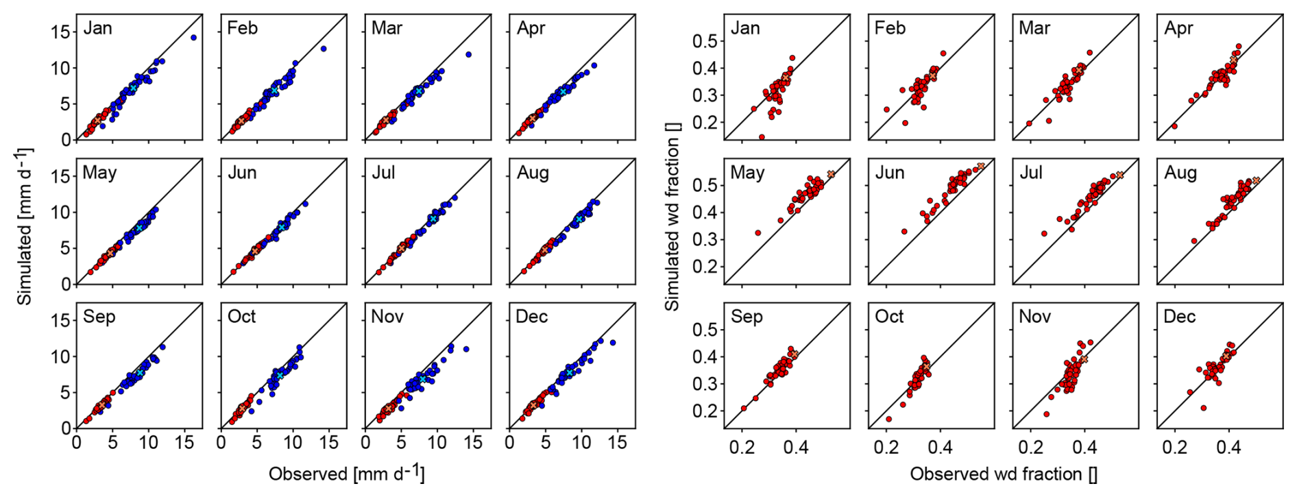
Figure 5 Same as Fig. 4 but for single stations within the Aare River catchment upstream of Bern (AarBrn). The crosses denote mean catchment all day and wet day precipitation and wet day frequency.

The following evaluation of the downscaling results refers to the catchment scale. A clear and concise evaluation is hindered by two aspects. First, the bias adjustment of temperature and precipitation was done using reference data spanning the periods 1991–2019 and 1991–2020, respectively, while the stochastic downscaling was trained using grid and station data over the period 1961–2019, and the analogs were built using station data over 1981–2019. We here use the periods 1991–2019 and 1981–2019 as reference. Second, the resulting 360 d calendar was built from the single RFs, which led to small shifts in some of the seasonal statistics presented.

For monthly mean precipitation (Fig. 6, first column), good agreement was found between observed and downscaled RF values for large and medium-sized catchments. Good agreement was also found for several small and very small catchments, while others – in particular Lonza, Saltina and Krummbach – showed notable differences for single months, with the mean observed annual cycle being outside the interquartile range (25th to 75th percentile) of the RFs.

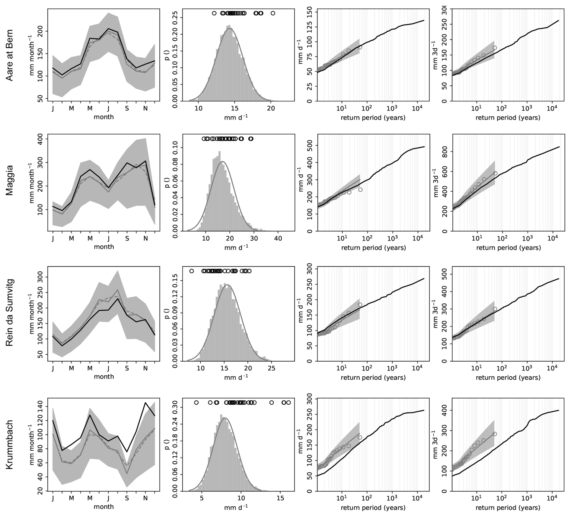
Figure 6 Evaluation of reforecast (RF) precipitation for selected catchments across different scale ranges: Aare at Bern (large), Maggia (medium), Rein da Sumvitg (small) and Krummbach (very small). From left to right: Annual cycle of mean monthly precipitation for observations (1991–2019, black) and RFs (grey; interquartile range (25th–75th percentile) in shading; mean based on 360 d calendar in dashed line); histogram of annual daily 90th percentile precipitation for RFs, and observations (black circles); return levels for annual maximum daily and maximum 3 d precipitation for RFs (black) and observation (grey circles) using the Gringorten plotting position. For observations, return levels have additionally been fitted using a Gumbel distribution (using a GEV distribution resulted in overly broad confidence intervals) and maximum likelihood estimates, confidence intervals are based on 5000 bootstrap samples (mean in dark grey, 2.5th–97.5th percentile in grey shading). Results for all test catchments are shown in Figs. S4–S7.

In terms of annual 90th percentile daily precipitation (Fig. 6, second column), good agreement was found between the observations and the RFs for large and medium-sized catchments. Specifically, the values for the single observed years lie within the distribution of the RFs. While the same is true for many of the small and very small catchments, observed values for single years are larger than all downscaled values for the Lonza, Saltina and Krummbach river catchments, and smaller than all downscaled values for the Rein da Sumvitg river catchment.

Annual maximum 1 and 3 d precipitation (Fig. 6, third and fourth column) show good agreement for the 29 years of observations used for large and medium-sized catchments, with the RFs falling within the confidence intervals of the observations. For 1 d maxima, the RFs show higher return levels for return periods greater than 10 years over the Thur river catchment at Jonschwil and at Andelfingen. For 3 d maxima, no such disagreement is noted. For 3 d maxima in the Inn and Kleine Emme river catchments, RFs indicate a smaller return value than observed above the 10-year return period. There is also a good agreement for several of the small catchments, however, over the Isorno river catchment, both 1- and 3 d maxima deviate strongly from the observed return levels. The largest differences are found over the very small catchments starting already at a return period of 1 year.

The analog method was used to disaggregate daily precipitation. Results over the catchments are mixed, also within catchments of the same scale range. For many of the large and medium-sized catchments, results indicate a relatively good overlap with the intensity-duration-frequency (IDF) curves of the observations, in particular for the 2-year return level, with the exception of the Sarine, Inn and Minster river catchments. For small and very small catchments, the downscaled RFs show overly strong precipitation intensities in particular for short durations. A detailed comparison of the full IDF curves is provided in Figs. S8–S11.

IDF curves for 1–7 d precipitation (Figs. S12–S15) show good agreement between the downscaled RFs and the observations for the 2-year return level for all large and medium-sized catchments, and the small catchments Allenbach, Drance de Bagnes and Thur at Alt St. Johann. The remaining catchments show larger differences. For some of the catchments showing a good performance, there are indications that higher return level precipitation episodes spanning several days are underrepresented (e.g., the 25-year return level over the Aare at Thun), whereas they are represented well for other catchments (e.g., the Sarine river catchment).

Figure 7 shows density plots based on annual and seasonal mean as well as daily mean temperature and precipitation for the large Aare River at Bern and the very small Krummbach River catchments. The observed seasonal and annual mean values (red crosses, rows 1, 2, 4 and 5) are within the density cloud of the RFs, except for single extreme years and seasons. For very small catchments, precipitation means tend to be closer towards the edge of the point cloud. Seasons in rows 1 and 4 were built using the RF forecasted days, while seasons in rows 2 and 5 are based on the 360 d calendar of the final time series. Not surprisingly, the concatenation of the single RFs to a 360 d calendar artificially increases seasonal variability, in particular for the transitional seasons. At the same time, observed extreme years indicated in the seasonal means are not depicted by the RFs, which is likely due to the opportunistic concatenation of the single RFs to yearly time series. Also for the remaining catchments there is overall a good agreement between RFs and observations. However, there are some indications of the RFs being slightly warmer than the observations in spring in the catchments of Thur (at Jonschwil and at Alt St. Johann), Maggia and Isorno. Density plots for all catchments examined are available in Figs. S16–S19.

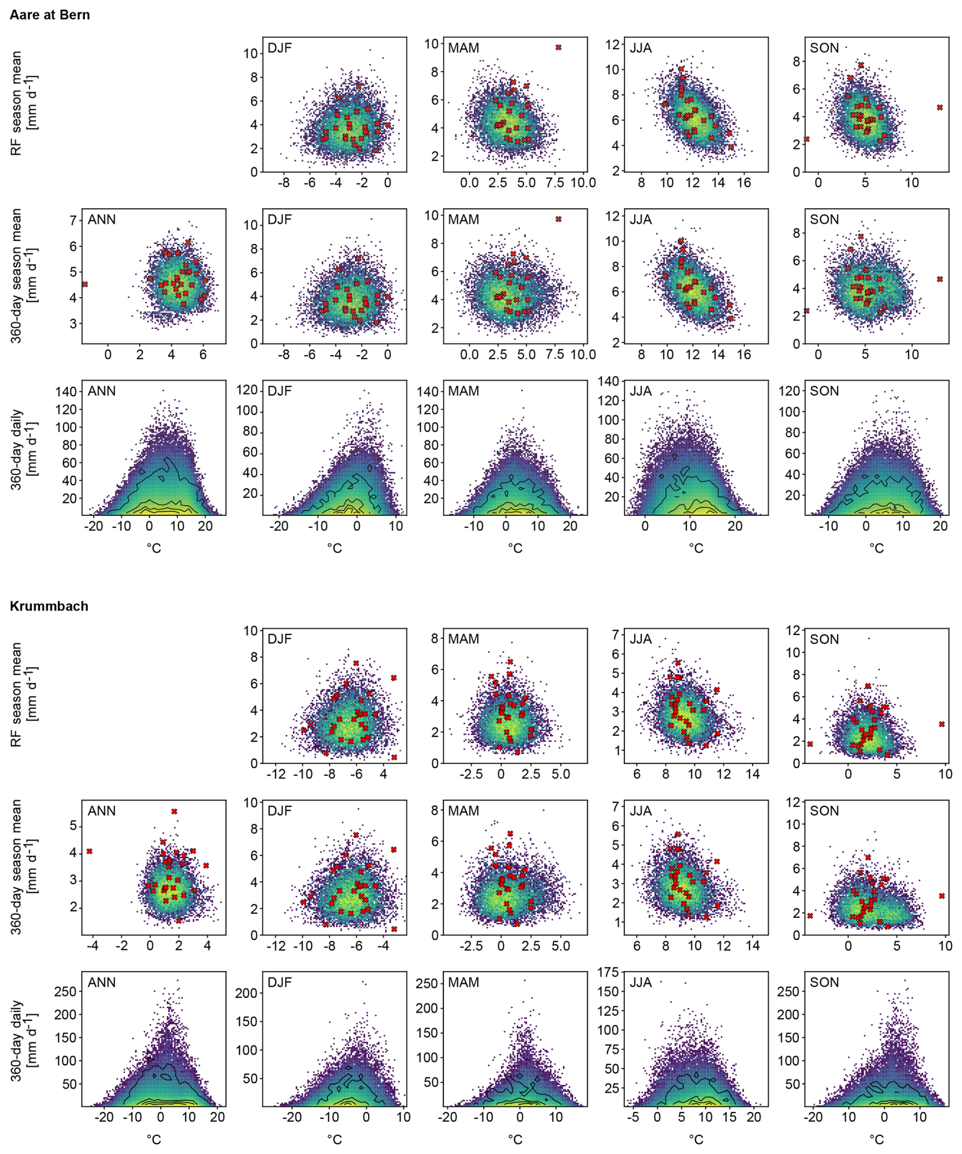
Figure 7 Density plots for the Aare River at Bern (top) and the Krummbach River (bottom), showing annual and seasonal precipitation and temperature based on seasonal means and the RF calendar dates (first row each), on seasonal means and the final 360 d calendar (second row each), and as based on daily means and the final 360 d calendar (third row each, days with a precipitation sum of ≥1 mm). Colours depict RF values, ranging from blue for low density to yellow for high density. Observations over the period 1991–2019 are denoted by red crosses (first and second row each) and contour lines (from low to high density in the innermost contours, third row each).

4.2 Hydrological validation

To assess the suitability of the bias-corrected and downscaled RFs for hydrological simulations, we derived flow duration curves (FDCs) from the RF-based simulations. Daily values were sampled over the length of the observational record, or the control run if shorter, from each block of 1000 years, and exceedance probabilities were computed separately. For visualisation, we calculated the 95 % confidence intervals for each exceedance probability over the flow values and show these together with the observations and the control run. Comparing the FDCs from RF, control run and observations for selected sites (Fig. 8), we find very similar behaviour for the Aare River at Bern, the Thur River at Andelfingen, and the Minster River. In contrast, for the Maggia River and, more pronouncedly, the Inn River, both RFs and control run yield higher flows than observed in the upper flow ranges. For the Maggia River, control run and RF-based simulation agree well to very well. The discrepancy to observations is partly or entirely due to the absence of the large flood events of 1981 and 1982 from the records, as the gauging station was destroyed during a severe flood in 1978, and measurements resumed only in 1995 (Näf-Huber et al., 2021). For the Saltina River, control run and observations agree well, whereas RFs show lower values overall, particularly in the upper flow ranges. This suggests limitations in the RF input for reproducing large floods in this small catchment.

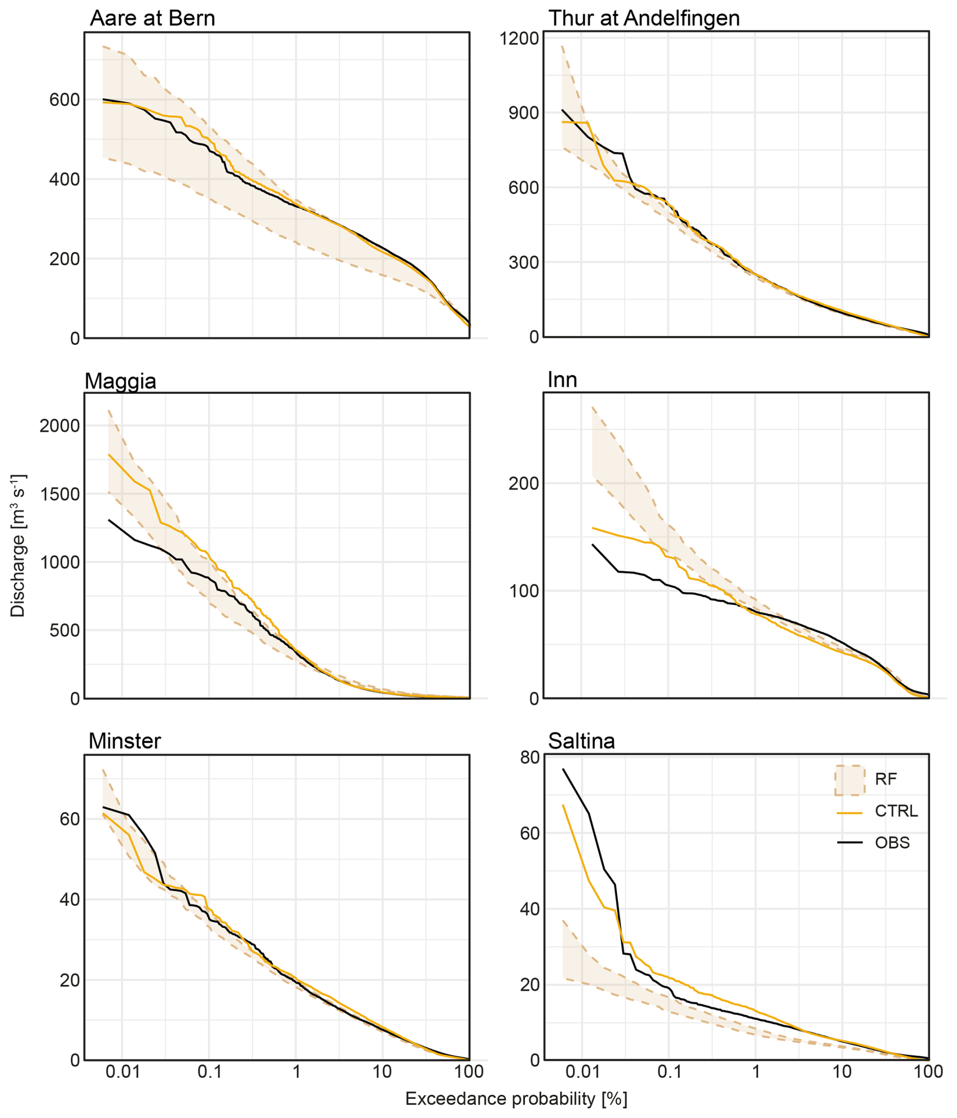
Figure 8 Flow Duration Curves (FDCs) for selected sites, comparing RF-based simulations (RF), control simulation (CTRL) and observations (OBS). Note that the x axis is scaled logarithmically. For RF-based simulations, samples matching the length of the observations (or, if shorter, the control simulation) were used to compute exceedance probabilities and corresponding 95 % confidence intervals.

We also examined the seasonality of AMF occurrence in the RF-based hydrological simulations and compared it with the seasonality in control run and observed AMFs at selected sites (Fig. 9). The months with frequent AMF occurrence are generally consistent, with differences typically no greater than one month. However, discrepancies are noted in the strength of AMF seasonality in some cases. For example, in the Inn River, RF-based AMFs are more evidently distributed across the months of frequent occurrence and do not show the pronounced peak in observed AMF occurrence centered in June, which is well captured in the control run. For the interpretation of all sites, it should be noted that the time periods and their durations for AMF observations, control run and RFs do not fully align.

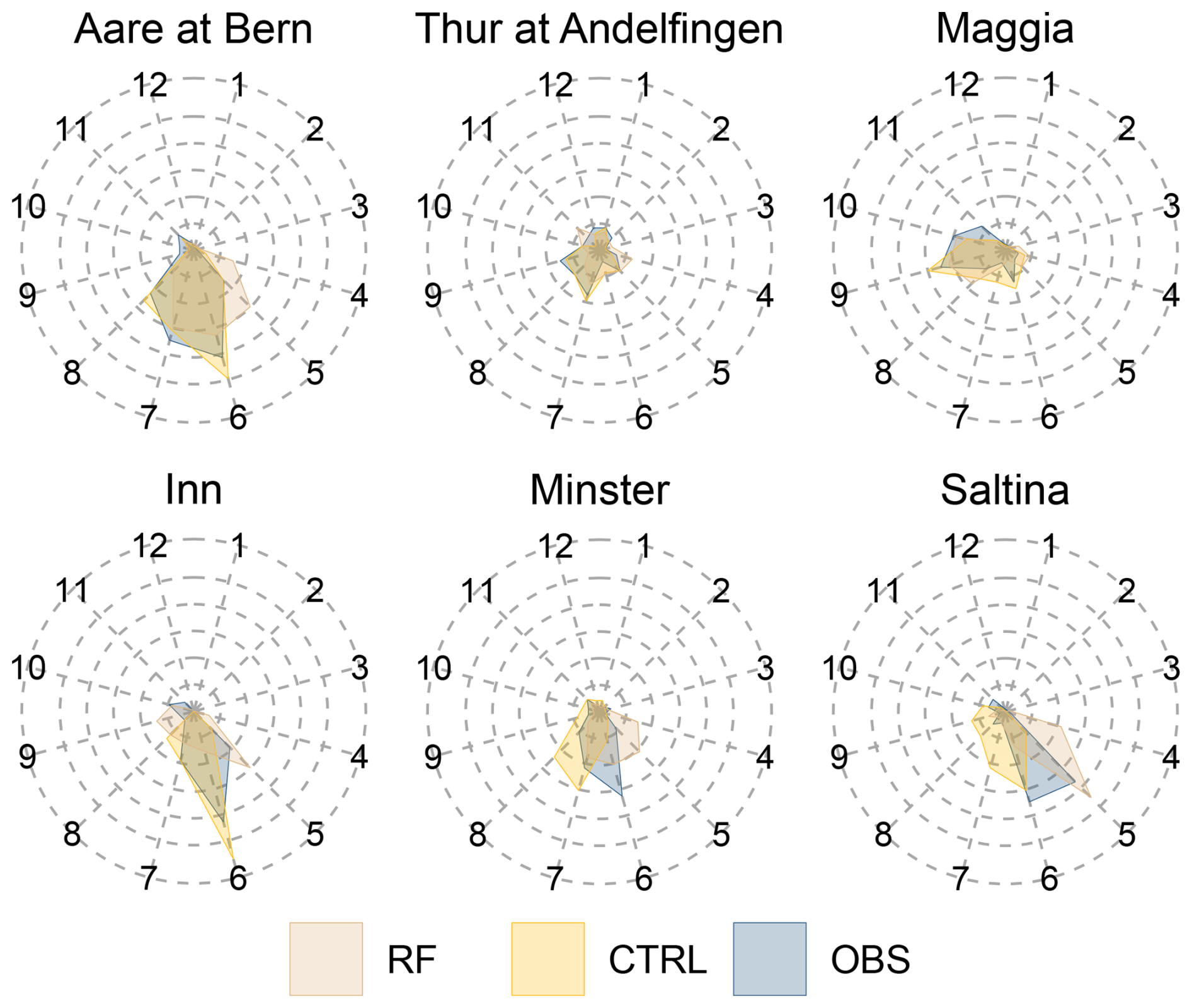
Figure 9 Seasonality of annual maximum floods for selected sites, comparing reforecast-based simulations (RF), control simulation (CTRL) and observations (OBS).

As individual RF segments were concatenated to obtain a continuous hourly time series (see Sect. 3.2.4), we verified whether the resulting AMFs do not show exceptional behaviour by comparing the time of occurrence and magnitude of the AMF with the stitching dates. For the smaller catchments, the densest occurrence of the AMFs is within a relatively narrow time window, occurring markedly after the stitching point, typically at least 100 d later. For the larger catchments, the AMFs are more widely distributed throughout the entire year following the stitching. In conclusion, the simulated AMFs appear to be unrelated in their magnitude and timing to the stitching points (see Fig. S20 for details).

4.3 Flood estimation results

Exceedance curves for selected examples are shown in Fig. 10. In the following, we compare RF-derived AMFs with observed AMFs, control-run AMFs simulated with observed weather for 1931–2019, and AMFs simulated using weather generator inputs (GWEX).

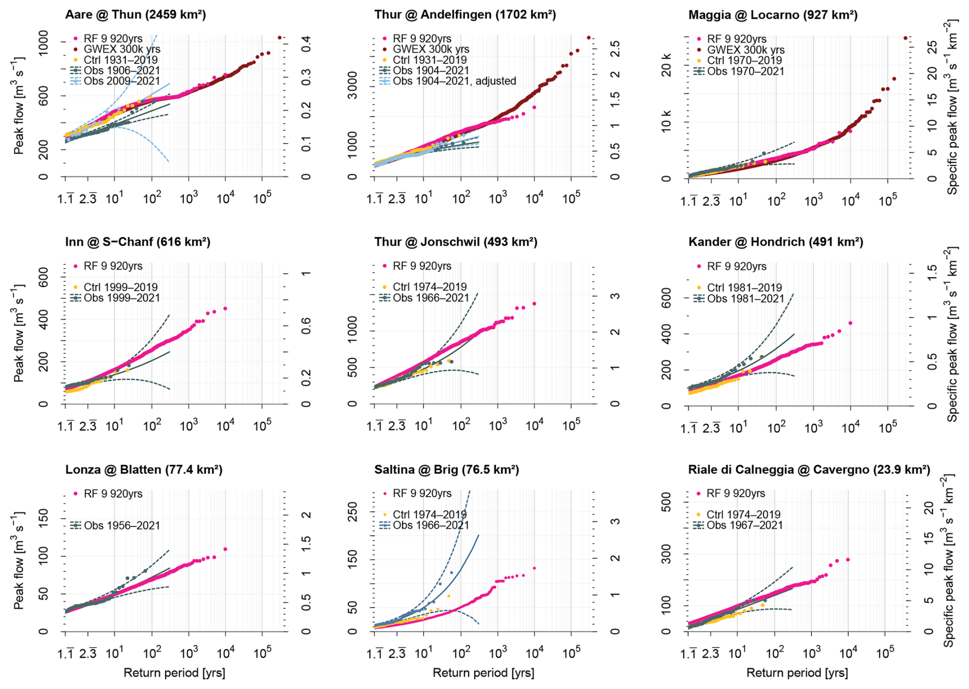
Figure 10 Exceedance curves from hydrological simulations using reforecast (RF) input. The top row shows three large catchments, for which long continuous simulations with input from the weather generator GWEX are available for comparison. The middle row shows three medium-sized catchments, the bottom row three small catchments. “RF” refers to annual maximum floods (AMFs) from the long continuous simulation (CS) based on reforecasts, “GWEX” to AMFs from the long CS based on weather generator input (only top row), “Ctrl” to AMFs from a control run with observed weather, and “Obs” are observed AMFs and a corresponding extrapolation.

Looking at large catchments (Fig. 10, top row), very good agreement between RF-based AMFs and observed AMFs is found for the Aare River at Thun. Note that the observed time series are not stationary at this site (Bundesamt für Umwelt (BAFU), 2020) because a flood relief tunnel was put into operation in 2009, and regulation rules for the upstream lakes Thun and Brienz were altered. The CS modelling chain used in this study depicts the current state, and comparison to observations of the period 2009–2021 is most appropriate, even though the statistics of observed floods from this period show an exceptionally wide confidence interval due to the short record length. Further downstream at Bern (not shown), return levels derived from RF simulations are higher than those based on observations and on the control run, whereas GWEX-derived AMFs show better agreement with observations. The discrepancy in the RF-based results is presumably due to an overestimation of flood contributions from smaller tributaries joining the Aare River. For the Thur River at Andelfingen, return levels from the RF-based simulation exceed those inferred from observations for return periods greater than approximately 5–10 years. The same is true for the control run and the GWEX-based simulation. However, at least three AMF measurements prior to 1998 were strongly influenced by bank overflow, before the river channel was modified to convey higher flows (Scherrer et al., 2011). An adjusted dataset incorporating reconstructions of unattenuated AMFs (Hunziker, Zarn & Partner, 2017) and the resulting flood statistics shows substantially better agreement with all simulations, which consistently represent the current, modified river state. For the large Maggia River catchment, which exhibits very challenging meteorological conditions, the RF-based flood exceedance curve agrees remarkably well with that of the observations. The highest AMFs simulated from RFs, with estimated return periods between 1000 and 10 000 years, reach values of approximately 5300–8400 m³ s⁻¹. The corresponding return levels estimated from GWEX are approximately 5500–9150 m³ s⁻¹, which is higher, but does not indicate a fundamental disagreement.

For medium-sized catchments (Fig. 10, middle row), we note curves lower (Kander River) or higher (Inn River, Thur River at Jonschwil) than observed exceedance curves.

For small catchments (Fig. 10, bottom row), results matching well with observations are possible, such as for the Riale di Calneggia and Lonza rivers. But as expected, marked underestimation can also occur, like for the Saltina River, where the highest RF-based AMF is only slightly higher than the highest observed AMF in the 55-year long records.

5 Discussion

5.1 Juxtaposition of reforecasts and weather generator precipitation

In the following, RF precipitation maxima are juxtaposed to the fundamentally different approach of constructing precipitation scenarios with the stochastic multi-site weather generator GWEX (see Sect. 2.5). Three catchments were selected for comparison as they well represent different conditions regarding climatology, station density and station representativeness: The Aare River at Bern, the Thur River at Andelfingen, and the Maggia River. These were evaluated in terms of annual peaks of areal precipitation, and three to four meteorological stations were selected per river basin (Table 3) with focus on different station elevations.

Table 3 Precipitation gauges used for juxtaposition with reforecasts and weather generator (GWEX), with coordinates (x,y) and elevation (z).

To achieve a consistent juxtaposition, a time series of 9900 years was taken each from RF and GWEX, and divided into 99 blocks with a length of 100 years each for computing confidence intervals. Observations (OBS) with a maximum length of 90 years in the period 1930–2019 were furthermore available for juxtaposition, with confidence intervals computed from a parametric bootstrap General Extreme Value (GEV) distribution fitted with L-Moments. The following discussion focuses on return periods that can be reasonably estimated from OBS, approximately 150 years according to the Gringorten (1963) plotting position.

As context for the juxtaposition, it should be noted that the RF data cover the years 1991–2020 and were bias corrected using RhiresD over this period. The stochastic downscaling was calibrated using the full available RhiresD dataset 1961–2019 and station observations from the same period. In contrast, GWEX was parameterized using OBS data from 1930–2019. Therefore, caution is warranted when comparing OBS, RF and GWEX, particularly given that the Atlantic Multidecadal Oscillation (AMO) index went through different phases between 1930 and 2019, indicating a relevant impact of internal climate variability (see also Sect. 5.4). The latest heavy precipitation statistics by MeteoSwiss (Fukutome et al., 2018, retrieved 27 March 2023) are shown for further reference. These use the entire measurement series available up to 2022 at each station, roughly compatible with the block length chosen for RF and GWEX.

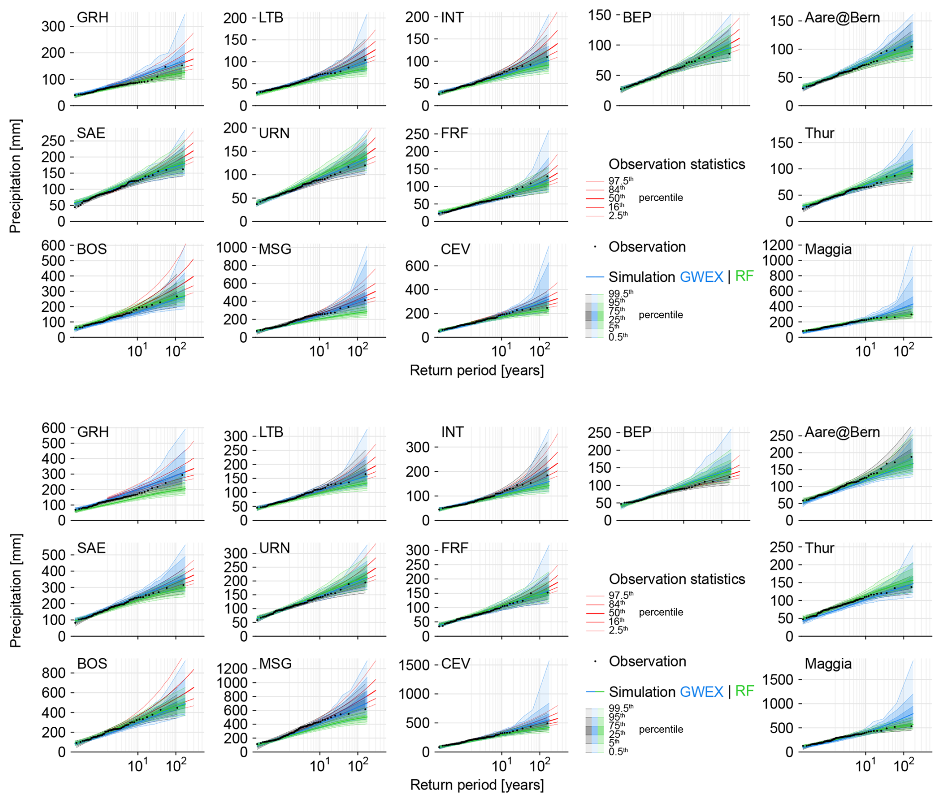
At-station maximum 1 and 3 d precipitation sums (Fig. 11, columns 1–4) generally show good to very good agreement between OBS, RF and GWEX for all three catchments considered. The largest disagreement is noted at the station Mosogno (MSG) in the Ticino River basin, where RF values are lower than OBS and GWEX. At the level of mean catchment precipitation, agreement is also high in all three river basins (Fig. 11, right). GWEX confidence intervals tend to exceed those of the RFs in the upper range of maximum 1 and 3 d precipitation sums for return periods larger than 50–100 years at both station and river basin level. This also means that GWEX in general reaches higher precipitation extremes in the 9900 years of data analysed as compared to the RFs. Given the differences between how the RF and GWEX time series are composed, it does not appear possible to draw firm conclusions beyond this statement. Also, comparisons with the observational range are not warranted, as the corresponding confidence intervals are derived from records of at most 90 years. Both for 1 and 3 d maxima, it is not possible to determine whether RFs or GWEX is closer to reality as regards high extremes.

Figure 11 Comparison of maximum 1 d (top) and 3 d (bottom) precipitation sums from reforecasts (RF), weather generator (GWEX) and observations (OBS). Columns 1–4 show selected precipitation gauging stations (see Table 3) within the full catchment shown in column 5.

5.2 Envelope curves for floods

Figure 12 shows an evaluation of the ten highest RF-based flood estimates in the context of maximum flood (Q_max) data from across Switzerland (Kienzler and Scherrer, 2018). Two envelope curves derived from these data are shown. Their slope was derived from a log–log linear regression, after which the intercepts were adjusted to encompass either all data or 95 % of the data, respectively. In addition, two relevant envelope curves for European data (Bertola et al., 2023), based on a regionally broader dataset, are shown. The global envelope curve by Herschy (2003) provides further context, as it includes data from substantially wetter climates and different hydro-climatic regimes.

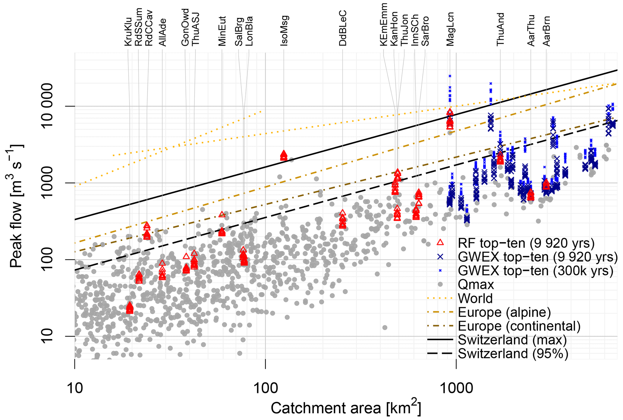
Figure 12 Highest ten annual maximum floods simulated using reforecast (RF) and weather generator (GWEX) input. Maximum observed floods in Switzerland as per Kienzler and Scherrer (2018) (gray dots) are shown for context, along with corresponding envelope curves (solid line: all data; dashed line: 95th percentile). Also shown are envelope curves for maximum floods in Europe (Bertola et al., 2023) (two regions are relevant: alpine, applies to AarBrn, AarThu, KEmEmm, MinEut, SarBro, ThuAnd, ThuJon; and continental, applies to the remaining catchments) and worldwide (Herschy, 2003). For catchment IDs see Table 1, for analyses separately for large river basins see Fig. S21.

Overall, the magnitude of RF-based maximum floods appears plausible, although they tend to be lower at smaller scales than expected from Q_max data and envelope curves. This is evident in catchments where storms increasingly dominate the generation of AMFs. Such catchments would require dynamical downscaling of RF, rather than stochastic downscaling, which was not feasible with the available data (see Sect. S1 in the Supplement). In contrast, RF-based maximum floods for the Ticino region – specifically for the Isorno River (IsoMsg, 124.7 km²) and the Maggia River (MagLcn, 926.9 km²) – are notably higher than in other regions. This is expected given the region's climatological characteristics, which favour particularly heavy precipitation events, as well as the crystalline bedrock, which promotes rapid and strong flood responses. In this context, it is interesting to note that the two highest RF-based maximum floods for the Maggia River exceed the Swiss envelope curve, and are comparatively close to the world record curve (note the logarithmic y axis), which contains data from wetter climates but is limited by record lengths and number of sites. The comparatively low values for the Aare River at Thun (AarThu, 2459 km²) and at Bern (AarBrn, 2941 km²) can be attributed to the marked attenuation of floods by Lake Brienz and Lake Thun further upstream, which is represented in the simulation chain but not in the envelope curve.

The highest ten GWEX-derived values from the full 300 000-year simulations often reach considerably higher magnitudes than those derived from RFs (again note the logarithmic y axis). This is not surprising given the substantially longer duration of the weather generator scenarios. However, when considering only 9920 years of GWEX weather scenarios – matching the length of the RFs – the magnitudes align more closely. Notably, the exceptionally high RF results for the Maggia River are consistent with GWEX results and remain plausible.

In the context of large river basins, the RF-based flood estimates align well with the regional patterns and are often positioned near the regional 95th percentile envelope. Values that are noticeably lower can be explained by lake retention in the case of the Aare River at Thun and Bern, as noted above, and by a combination of slightly different climatological regime and small catchment area in the case of the Krummbach (KruKlu), which is the smallest test catchment considered. Compared to other large river basins, flood estimates for sites not influenced by lake attenuation fall somewhat more noticeably below the regional 95th percentile envelope in the Aare River basin. Full regional envelope curves are provided in Fig. S21.

5.3 Flood return levels

Some caution is warranted when interpreting the estimated return periods of AMFs derived from the RF-based long CS: although the individual RF ensemble members are assumed independent after discarding days 1–15, their ability to accurately represent the flood-relevant meteorological behaviour across different regions cannot be examined systematically with the test catchments used in this proof of concept. The exceedance curves for the larger test catchments, however, indicate a generally plausible range when compared to observed AMFs and their extrapolation. However, it should be borne in mind that the observed AMFs are also subject to uncertainty (Westerberg et al., 2020), and that the available observed AMFs are instantaneous peak values, as opposed to the hourly simulated values.

An important question that RF-based model runs can help address is how the exceedance curve behaves as the return period increases. Notably, the observed AMFs sometimes appear to level off, whereas GWEX-derived AMFs typically do not. Interestingly, the RF-derived AMFs also generally show no levelling off or a tendency towards a plateau value. Moreover, the agreement between RF and GWEX-based flood estimates in the tail is remarkably high where comparison can be made (Fig. 10), particularly also in the case of the Maggia River, which shows an exceptionally heavy tail. This general agreement is noteworthy because the RFs offer a more physically based approach to precipitation scenarios, whereas the GWEX weather generator employs a stochastic approach without explicit physical boundary conditions. This suggests that indeed the AMF observations – paired with extrapolation using a GEV distribution – might underestimate the potential of catchments to generate increasingly higher floods within the return periods considered here. This interpretation is preliminary, as the range of test catchments examined in this study is limited, and the return periods covered extend only to 1000–10 000 years.

It should be noted that the RF-based exceedance curves primarily reflect the internal consistency of the chosen modelling chain. Structural and epistemic uncertainties inherent to the numerical weather prediction system, such as systematic biases in extreme precipitation or storm dynamics, remain largely unresolved (see Sect. 5.4.8). Consequently, the RF-derived return levels should be interpreted as conditional on the applied RF ensemble and postprocessing framework.

5.4 Limitations

Several limitations of the current approach should be considered when interpreting the results.

5.4.1 Interpolation

Methods such as Thiessen interpolation of point values, precipitation adjustment factor and temperature lapse rates were applied to enable exceedingly long CS within the EXAR and EXCH project frameworks (Viviroli et al., 2022) (Sect. 3.3). Along with statistical RF downscaling, these methods have limitations for smaller catchments, which however were not the focus of EXAR and EXCH but here serve to explore the RF-CS approach across a broad range of scales from approximately 20–3000 km². Addressing some of the associated complexities – such as through dynamical downscaling, targeting mean areal precipitation and temperature, or even a spatially distributed modelling approach – will be time-consuming and require further research. In particular, dynamical downscaling could improve representation of short-duration, small-scale precipitation extremes. However, due to the coarse temporal resolution of the available RF data and the high computational demand, it was not feasible for the long multi-millennial series considered here (Sect. S1). For large-scale extremes, stochastic downscaling remains adequate, while dynamical approaches could be applied in the future if higher-resolution data become available.

5.4.2 RF resolution

Further limitations are related to the resolution of the RF data. Initially, we planned to use both the ENS Model Climate (day 1–15) and the Extended Range Model Climate (day 16–45) for the statistical downscaling. However, due to inconsistencies in the data and concerns about the independence of short forecasting times from observed weather, only the Extended Range Model Climate data were used (see Sect. 2.2), effectively discarding days 1–15. In consequence, the statistically downscaled time series were only 9920 years long. On the other hand, ENS Model climate data are available at 0.25° resolution, whereas the longer forecasts are available on a coarser 0.5° grid, limiting the applied approach in terms of catchment size.

5.4.3 RF evolution

Since its introduction, the ECMWF IFS and hence the RFs have undergone continuous updates (see Sect. 2.2). When building the yearly time series required for the hydrological modelling, we were drawing from RFs initialised in the same year. For many initialisation years, this resulted in concatenation of RFs from different IFS cycles. Certainly, over the 12 initialisation years of RFs, considerable model evolution has occurred. However, while the extent of updates between successive IFS cycles varies, the updates are gradual, often introducing only minor changes. The resulting yearly time series are hence, at most, based on slightly different IFS model versions.

5.4.4 Small and very small catchments

While results of the statistical downscaling approach match well with observations for medium and large catchments, the stochastic downscaling is not well suited for very small catchments, where only a few stations are scattered over few or even only one grid-point. The Extended Range Model Climate RFs used have a spatial resolution of 0.5° ($\sim \mathrm{38}\times \mathrm{56}=\mathrm{2128}{\mathrm{km}}^{\mathrm{2}}$ in the study domain), whereas some of the catchments examined cover an area of less than 50 km², and only 2–3 stations were used in the calibration of the stochastic downscaling. We noted a systematically poor performance for these catchments. The smaller number of stations, together with the coarse resolution of the RFs, impedes the estimation of reliable statistical relationships between the large and small scale during the calibration of the stochastic downscaling.

5.4.5 Temporal disaggregation

For the temporal disaggregation, we have experimented with several procedures to draw the best analogs. Additionally, we initially planned to disaggregate temperature using the analog method, alike precipitation. Approaches tested included mean daily temperatures, absolute values of temperature and differences between minimum and maximum temperatures at the station level. All of these approaches led to very strong temperature jumps when the single RFs were concatenated to the yearly time series. To smooth those steep changes from one hour to the next, we pragmatically interpolated between the bias corrected 6-hourly temperature values. For precipitation, the applied analogs performed satisfactorily for large and medium-sized catchments, but showed excessive precipitation intensities in particular for short durations and in small to very small catchments.

5.4.6 Sampling of interannual variability

The concatenation of individual RFs to yearly time series furthermore disregarded other potentially more important aspects. Future efforts could seek to additionally incorporate variables accounting for the dynamic state of the atmosphere such as geopotential height, and aim at sampling inter-annual variability which might require the reuse of single RFs when building the annual time series. However, comparison of observations and RFs on a seasonal and annual scale indicated that the time series produced do not contain years with values overly above or below observed precipitation and temperature.

5.4.7 Sampling of long-term internal variability

The RFs were introduced in March 2008, reforecasting weather up to 18 years prior. Considering full years only, the RFs used in this study span the period 1991–2019 (excluding 2015, see Sect. 2.2), with fewer data at the beginning and end of this period and more in the middle. Counting the number of RF days per month and year indicated that the Atlantic Multidecadal Oscillation (AMO) was predominantly in a positive phase during the RF period (see Trenberth et al., 2023), particularly in the middle of the period when the largest number of RFs were available. This results in oversampling of positive AMO phases in the RFs processed here. A detailed figure of AMO phases and RF sampling is provided in Fig. S22.

5.4.8 Structural and model uncertainty of reforecasts

Although the RF-based time series of nearly 10 000 years provides a robust estimate of sampling variability, it is important to note that all realizations share the same model physics, parameterizations, and structural assumptions. Increasing the number of RF realizations can therefore not reduce epistemic or structural uncertainty inherent in the underlying numerical weather prediction system. Similarly, minor inhomogeneities arising from the continuous evolution of the underlying forecast model cannot be fully eliminated, despite the mitigation steps described in Sects. 2.2, 3.2.1 and 3.2.4. Systematic biases in precipitation extremes, storm persistence, or co-variability of temperature and precipitation are propagated into the hydrological simulations. Bias correction and stochastic downscaling adjust marginal statistics but do not fully address errors in event dynamics, spatial coherence, or representation of processes relevant for extreme floods. Consequently, the narrower confidence intervals of RF-based precipitation extremes compared with GWEX (see Sect. 5.1) primarily reflect internal consistency of weather model and postprocessing. Interpretations of RF-based flood return levels should therefore be considered conditional on the modelling framework and postprocessing applied, with the relative importance of uncertainty sources depending on catchment characteristics such as size, elevation, geology, climatology and human disturbance (see Kritidou et al., 2026).

5.4.9 Non-stationarity

With ongoing climate change, mean precipitation over the Alps is projected to increase during winter and decrease during summer. Virtually all state-of-the-art global and regional climate model ensembles indicate an increase in extreme precipitation over the Alpine region, except for summer, where only high-resolution global climate models and regional climate models indicate an increase (Ritzhaupt and Maraun, 2023). The RF simulation period spans 1991–2019, which was also used for the bias adjustment. The RFs are thus representative for the current state of the climate, whereas aspects of non-stationarity are not accounted for. Given the dominant role of precipitation for the subsequent hydrological simulations (Kritidou et al., 2025), any resultant flood estimates should be re-assessed within a time-frame of approximately 10 years.

6 Conclusions

This study evaluated whether ECMWF reforecasts (RFs) can be transformed into meteorological inputs suitable for long continuous simulation and derived flood estimation in a challenging Alpine environment, addressing three research questions.

Regarding the feasibility of processing and concatenation, we demonstrated that bias adjustment, stochastic downscaling and temporal disaggregation allow the construction of consistent hourly forcing data from RF data. Individual RF segments can be concatenated into multi-millennial sequences, and the stitching points do not systematically influence simulated AMFs. Hydrological validation further showed that the simulated discharge series reproduce the frequency of daily discharge magnitudes and the distribution of Annual Maximum Floods (AMFs) with sufficient realism for flood frequency analysis. For large and medium-sized catchments (larger than approximately 500 km²), performance ranged from satisfactory to good, while limitations were identified for small and very small catchments. These scale-dependent limitations primarily reflect constraints of the statistical downscaling approach applied. Processing for the largest catchments was completed within a few hours, confirming that the approach is feasible also in terms of computational cost.

Regarding comparison with and complementarity to an established stochastic weather generator approach, the RF-based flood frequency estimates are comparable to those of the weather generator approach and do not suggest systematic underestimation of rare yet unobserved floods. The RFs thus provide an independent and physically based complement to the purely statistical approach of the weather generator, as they are initialised with observed states and evolve according to model physics.

Regarding limitations specific to the RF-based approach, three issues should be acknowledged. First, RFs inherit structural uncertainties in the underlying numerical weather prediction system, which may affect the realism of simulated extremes and cannot be removed through statistical postprocessing. Second, the RF archive does not explicitly account for long-term climate variability or non-stationarity, introducing uncertainty when constructing multi-millennial synthetic sequences. Third, the spatial and temporal resolution of the RFs, together with the applied stochastic downscaling approach, constrains their applicability in small and very small catchments, where small-scale precipitation variability strongly controls flood generation.

Snowmelt-related processes were not analysed explicitly, as AMFs in the study catchments predominantly occur during summer convective events when rainfall dominates flood generation (see Viviroli et al., 2025). Extending the framework to explicitly assess temperature- and snowmelt-related return periods represents a relevant topic for future research (see, e.g., Staudinger et al., 2025, in the context of continuous simulation and extreme floods).

Several methodological developments could further improve the applicability of the framework. In particular, extending the stochastic downscaling to higher resolved temporal data should be explored. In this proof-of-concept study, a key limitation was data availability, particularly with respect to gridded observations at high temporal resolution. The hourly CombiPrecip dataset, for example, currently extends only from 2005 onward, although the record will eventually reach the length required for use as a predictor dataset for stochastic downscaling calibration. In the meantime, alternative approaches for generating sub-daily variability could be explored in place of the analog-based method applied here, for example through stochastic disaggregation methods (Kossieris et al., 2018).

To improve results in small and very small catchments, the potential of dynamical downscaling should also be further explored, provided that RF data become available at higher temporal and spatial resolution.

Other possible avenues to derive local information from RFs include the use of emulators (see Maraun and Widmann, 2018, for an overview). Doury et al. (2023, 2024) proposed a regional climate model (RCM) emulator that combines empirical statistical downscaling methods with dynamical downscaling through a neural network architecture and could be applied directly to the RF data. In combination with recent convection-permitting modelling efforts such as the CORDEX FPS on convective phenomena over Europe and the Mediterranean (Ban et al., 2021), such emulators could improve the representation of local-scale extremes.

Overall, the processed ECMWF RFs provide a viable and computationally efficient meteorological forcing for long continuous simulation in Alpine catchments at medium to large spatial scales. Their added value lies in being physically based rather than statistically derived, which allows RF-based flood estimates to serve as a process-based counterpart to approaches based on weather generators.