Future rime ice conditions for energy infrastructure over Fennoscandia resolved with a high-resolution regional climate model

Societies today are increasingly reliant on electricity, underscoring the need for reliable energy production. In cold climate regions, ice accumulation can cause significant harm to structures such as power transmission lines, leading to power loss or, in the worst case, the collapse of wires or transmission towers. Thus, since climate change is expected to impact winter weather conditions in northern Europe, its effects on atmospheric icing occurrence over the Fennoscandian region is a crucial area of study. Here, we utilize an ice accretion model based on ISO 12494, driven by outputs from the high-resolution regional climate model HCLIM, to analyze in-cloud icing conditions over two future 20-year periods: mid-century (2041–2060) and end-of-century (2081–2100). The regional outputs are bounded by two global climate models (EC-EARTH and GFDL-CM3, respectively) under the highly warming RCP 8.5 emission scenario. The results, both from the whole Fennoscandian area and from specific regions relating to energy infrastructure, suggest a general decrease in in-cloud icing conditions over northern Europe compared to the historical period (1986–2005). An exception lies in the northern parts of Fennoscandia and locally over higher altitudes, where some increasing trend is seen, particularly for annual maxima. Under the RCP 8.5 scenario, freezing temperatures become less common; however, rising temperatures allow for more moisture, potentially enhancing in-cloud icing if sufficiently cold temperatures remain.

1 Introduction

Atmospheric icing poses significant challenges for various sectors in cold climate regions globally. Energy infrastructure, in particular, is vulnerable to disruptions due to ice accumulation on power transmission lines or wind turbines (Hämäläinen and Niemelä, 2017; Zhou et al., 2011; Chang et al., 2007; Frick and Wernli, 2012). For wind turbines, ice on the blades disturbs power production and accelerates blade wear, while transmission lines can experience problems such as galloping, and consequently, wire and tower breakage due to the combined effect of strong winds and icing (Chen et al., 2022; Havard and Van Dyke, 2005). Moreover, icing can reduce the efficiency of energy transmission by contributing to a phenomenon known as corona loss (Sollerkvist et al., 2007; Yin et al., 2017; Lahti et al., 1997), in which the air surrounding a conductor is ionized and a corona discharge occurs.

Atmospheric icing has been studied for nearly a century (Arenberg, 1943; Lewis et al., 1947). It is an umbrella term that encompasses multiple types of ice accretion: rime ice due to supercooled liquid cloud droplets, glaze ice forming primarily by accretion of freezing rain or drizzle, and wet snow icing due to adhesion of wet snow or sleet just above freezing conditions (Makkonen, 2000). Suitable conditions for ice accretion depend on several meteorological parameters such as air temperature, cloud liquid water content, wind, and precipitation. Climate change is projected to alter their distribution in mid-latitudes, particularly during the winter season (Lind et al., 2022); increases in temperature, moisture, and precipitation are expected. Thus, changes in the occurrence of atmospheric icing are anticipated in Finland and the broader Fennoscandian region, as has been discussed in previous research (Lutz et al., 2019; Iversen et al., 2023).

Both Lutz et al. (2019) and Iversen et al. (2023) examined how rime ice conditions – and in Iversen et al. (2023)'s case, also wet snow conditions – are projected to evolve from the perspective of power transmission lines. Iversen et al. (2023) utilized the regional weather model known as WRF (Weather Research and Forecasting) with a horizontal resolution of 12 km to downscale two climate model configurations, furthermore assessing the changes in rime ice and wet snow loads. For rime ice, the largest changes were predicted over the Scandinavian mountains, with differing trends between the two configurations; over western Finland, a mostly decreasing trend was noted. Iversen et al. (2023) recommended an ensemble approach for planning future ice load designs.

Lutz et al. (2019) employed an ensemble approach, using the output of 11 regional EURO-CORDEX climate simulations with 12 km resolution to assess the change in icing on power lines. The simulations were a combination of six global climate models (GCM) and three regional climate models (RCM). They found predominantly increasing trends in northern Finland, with mixed signals for southern and central Finland. They concluded that the regional climate model had more effect on the results than the global climate model through the influence of cloud liquid water on icing. However, cloud liquid water content was not included in the EURO-CORDEX simulations, and therefore they had to estimate it from relative humidity (for cloudiness), specific humidity (water content), and temperature (fraction of liquid water). Other studies on the impacts of climate change on icing conditions have focused mainly on cases related to wet snow or freezing rain (Kämäräinen et al., 2018; Rácz et al., 2022; Marinier et al., 2023).

In this paper, we utilize outputs from a high-resolution regional climate model HARMONIE-Climate (HCLIM), with boundaries from two global climate models, to assess changes in in-cloud icing over the Fennoscandian region. The research has been conducted under an EU HORIZON project called RISKADAPT (Asset Level Modelling of Risks in the Face of Climate Induced Extreme Events and Adaptation) with a focus on power transmission lines, similarly to previous research on the topic. However, we can simulate atmospheric icing at multiple lower tropospheric heights (50–400 m) which also allows us to assess the risks of in-cloud icing for wind production. In addition, we can simulate icing at a higher horizontal resolution than before (3 km vs. 12 km in both Iversen et al., 2023, and Lutz et al., 2019). It is important to note that a high horizontal resolution comes at the expense of reducing the ensemble size and usually shorter time periods. Results at the height of 50 m, closest to the surface used in this study, are presented for northern Europe and two areas in Finland, highlighting the perspective of power transmission lines. For wind energy, results are presented from five areas coinciding with areas of wind energy production around Fennoscandia.

The paper is divided as follows. Section 2 details the icing model, climate model outputs, and icing data processing. Section 3 presents the main results. They cover changes in mean and annual maximum ice masses across Fennoscandia, along with regional results focusing on either transmission lines or wind energy. In addition, changes in input parameters such as temperature are inspected to better discuss the results and present conclusions in Sects. 4 and 5.

2 Data, models, and methods

2.1 Rime ice model

Based on the icing algorithm of Makkonen (2000), a rime ice model has been developed at the Finnish Meteorological Institute and has been used, for example, to create an icing atlas for wind park planning (Hämäläinen and Niemelä, 2017). Rime ice accretion is modeled over a vertical (length = 1 m, diameter = 0.03 m), freely rotating standard cylinder with icing rate (g s⁻¹) as its main output:

$$\begin{array}{}\text{(1)}& {\displaystyle \frac{\mathrm{d}m}{\mathrm{d}t}}={\mathit{\alpha }}_{\mathrm{1}}{\mathit{\alpha }}_{\mathrm{2}}{\mathit{\alpha }}_{\mathrm{3}}w\mathit{v}A,\end{array}$$

where α₁ is the collision coefficient, α₂ the sticking coefficient and α₃ the accretion coefficient, while w stands for the liquid water content (g m⁻³), v denotes wind speed and A the surface area of the cylinder. In other words, the algorithm represents how well the cloud droplets (w) carried by the air stream (v) aggregate (α₁, α₂ and α₃) to the cylinder (A).

Drag and inertia control how well the particles in the air stream hit an object. This is represented by the collision coefficient α₁, which is close to 1 for large particles (for which inertia dominates) and close to 0 for small particles. The size of the particles depends on the median volume diameter (MVD), which itself is dependent on the liquid water content and the cloud droplet number concentration Nd. In this study, Nd was set as constant, 100 cm⁻³, as reasoned by Hämäläinen and Niemelä (2017).

The sticking coefficient α₂ expresses how efficiently air particles freeze upon contact with an object. In cases of rime ice, we are interested in supercooled water droplets that freeze immediately without rebounding; the same applies approximately for cases with rain droplets, so α₂ is set to 1. The accretion coefficient α₃ differs for dry growth cases (where α₃ = 1) and wet growth cases (where there is a liquid layer on top of the ice surface; α₃ < 1). The international standard explains in more detail how these wet growth cases are managed in accordance with the accretion coefficient (International Organization for Standardization, 2017). The melting process in the ice model begins when the air temperature rises above 0 °C.

From icing rate, various parameters related to icing are calculated; most notably the ice mass (g m⁻¹), but also the ice density (g m⁻³), the total diameter of the cylinder and ice (Makkonen, 1984; Makkonen and Stallabrass, 1984).

2.2 HARMONIE-Climate

Our study aims to investigate future icing conditions in the Fennoscandian region; thus, regional climate model projections are required as input to the rime ice model. HARMONIE-Climate (HCLIM) was chosen for this purpose because it provides all the necessary parameters to model rime ice in a high horizontal resolution.

HCLIM is based on the numerical weather prediction (NWP) model configuration of the ALADIN-HIRLAM NWP modeling system (Belušić et al., 2020; Lindstedt et al., 2015). Experiments by the Nordic Convection Permitting Climate Projections project (NorCP; Lind et al., 2020) have been conducted with the HCLIM regional climate model in northern Europe using HARMONIE-Climate cycle 38 in two configurations: a lower resolution configuration (12 km) utilizing the ALADIN physics package (Termonia et al., 2018) and a higher resolution configuration (3 km) where deep convection is resolved (Bengtsson et al., 2017). Data from the latter were used in this study; the required parameters were calculated for multiple lower troposphere levels (50, 100, 200, 300, and 400 m) with a horizontal resolution of 3 km and a temporal resolution of 3 h. High horizontal resolution has its drawbacks, as it limits the ensemble approach due to the high computational costs of running the RCM.

RCMs require information on lateral boundary conditions, which are provided by large-scale global climate models. The HCLIM output we used was based on two boundary GCMs from the Coupled Model Intercomparison Project-Phase 5 (Taylor et al., 2012), EC-EARTH and GFDL-CM3, chosen specifically to capture different types of climate response (Lind et al., 2022). Although both GCMs project warming and increased humidity in northern Europe due to climate change, the response is more intense in GFDL-CM3 compared to EC-EARTH.

HCLIM output had been generated for three time periods spanning 60 years in total; a control run from the historical period (1986–2005), a mid-century run (2041–2060), and an end-of-century run (2081–2100). These are referred to as historical, mid-century, and end-of-century, respectively hereafter.

In this study, we used the precalculated HCLIM dataset with Representative Concentration Pathway (RCP) emission scenarios RCP 4.5 (moderately warming) and RCP 8.5 (strongly warming). Since RCP 4.5 data was available only with one boundary model (EC-EARTH), scenario RCP 8.5 was selected allowing the use of two climate model datasets with different lateral boundaries (EC-EARTH and GFDL-CM3). The RCP 8.5 concentration pathway assumes continuously rising greenhouse gas emissions throughout the 21st century. Although RCP 8.5 may be considered to be increasingly unlikely due to the overestimation of coal use by the end of the century (Freistetter et al., 2022), it remains a useful tool for mid-century policy assessments (Schwalm et al., 2020).

Temperature, wind speed and liquid water content are the three primary output parameters used as an input for the rime ice model presented above in Sect. 2.1. In their paper, Lind et al. (2022) provide different levels of information on the validity of the output data. For temperature in 2 m, they report that the biases in wintertime are generally small, with a median bias of about −0.5 °C for EC-EARTH based simulations and +1 °C for GFDL-CM3 when compared with ERA5 data. Furthermore, the changes in daily maximum and minimum temperatures across the time periods are statistically significant. For wind speed, the changes are less robust, and liquid water content has not been validated.

Liquid water content (LWC) in an atmospheric layer can be divided into cloud liquid water content (CLWC) and rain liquid water content (RLWC), so into nonprecipating cloud droplets and rain droplets (Tian et al., 2019; Ellis and Vivekanandan, 2011). As HCLIM bases its cloud microphysics in an ICE3-OCND2-scheme, the model would be able to separate hydrometeors between cloud water and rain (Lind et al., 2020; Bengtsson et al., 2017). However, the simulations we used as input data only included the cloud liquid water content (CLWC), meaning that no icing from precipitating hydrometeors was modelled in our research.

2.3 Methods

2.3.1 Processing of the ice model output

The icing model output was further processed to allow a comprehensive evaluation of the changes in icing climate from multiple perspectives. The results can be divided into two categories: (1) results calculated for 50 m above ground to investigate icing on power lines, and (2) results calculated for multiple lower tropospheric heights (50–400 m) relevant for wind energy production. The altitude of 50 m was chosen for power lines as it was the lowest height above ground level where HCLIM output data were available. Table 1 lists the evaluated parameters and details the domains and heights they were analyzed at. In addition, we focused only on the months when freezing temperatures are common in northern Europe (October to April) in our analysis, following the example of Iversen et al. (2023).

Table 1 Post-processed parameters and the domains for which they have been calculated are listed here. The locations of areas 1–7 can be found in Fig. 1.

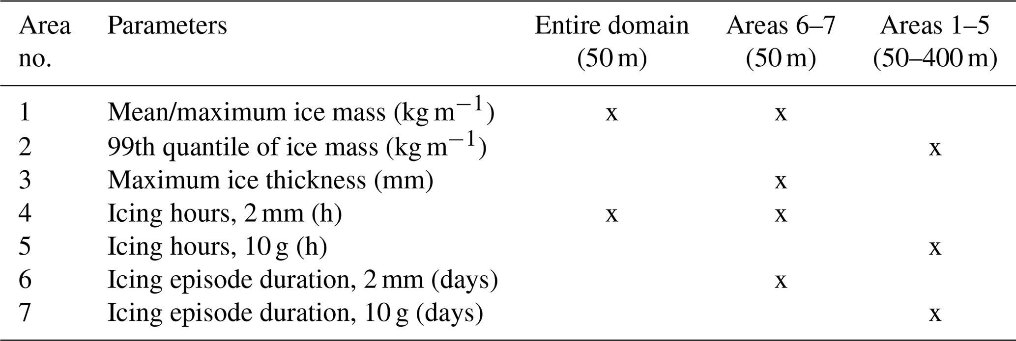
Figure 1 displays the specific areas referenced in Table 1, while supplementary information on the areas, including the relief information, are shown in Table B5. Each area is named according to the municipality or one of the municipalities they fall under. In areas 1–5, which were selected to coincide with existing or planned wind parks, results were calculated for all heights. For power line perspective, separate areas were selected (areas 6–7) and in these regions only results at 50 m height were considered. In areas 6–7, the maximum of all the grid points in the area was determined for each time step, and additional parameters were derived from that, including annual mean and maximum ice masses and icing episode durations. An icing episode is defined as the number of days the ice cover thickness stays over 2 mm. This limit is based on earlier research (Lahti et al., 1997) relating to corona losses caused by icing. In addition, when calculating the annual average of icing hours for the entire Fennoscandian area, 2 mm was used as the threshold for defining an icing hour.

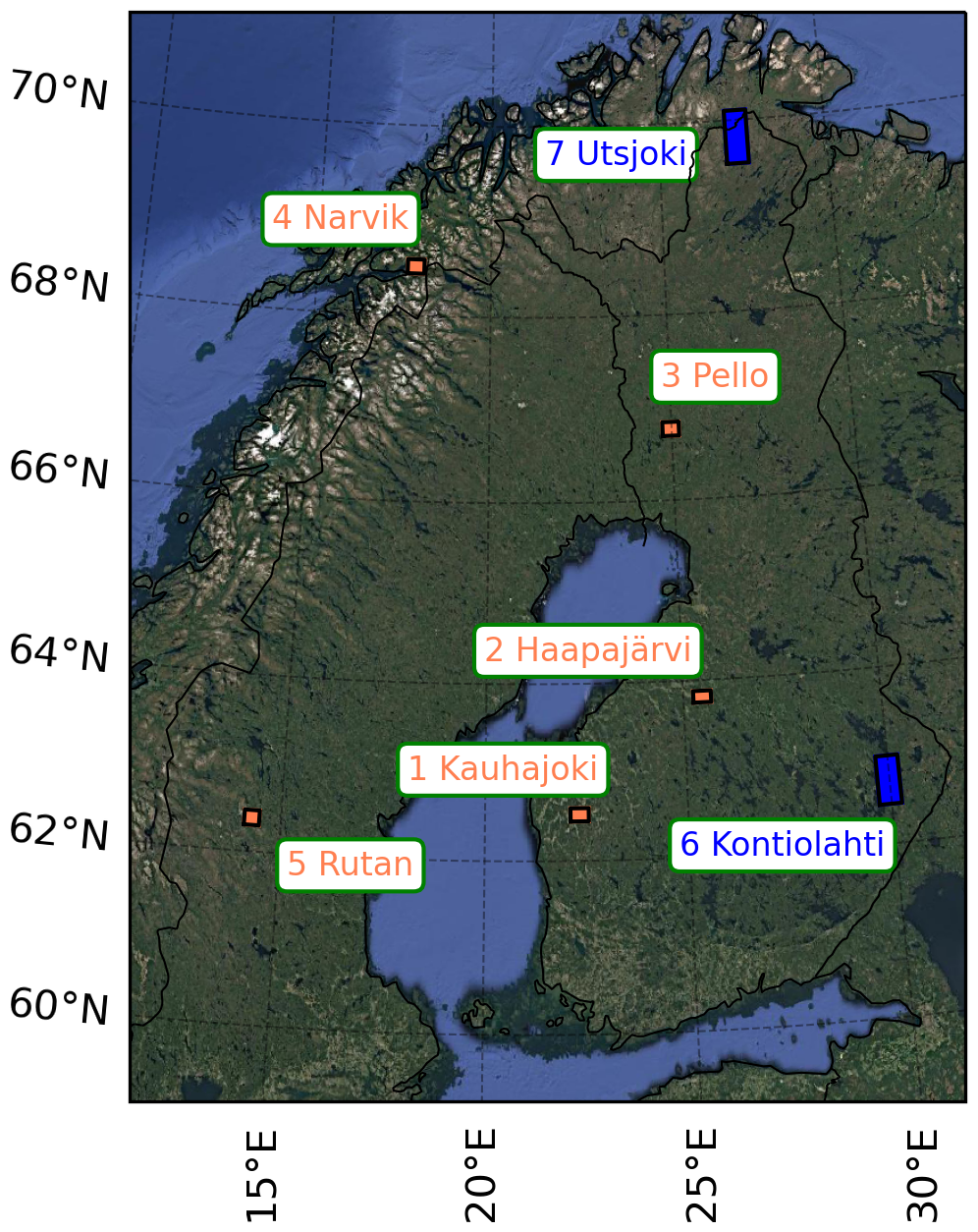
Figure 1 Map showing the locations to which specific results have been calculated. Marked with orange, areas 1–5 are regions where all heights have been considered and they align with existing or planned wind parks. Marked with blue, areas 6–7 are regions where results were calculated only at 50 m with a focus on power transmission lines (Map data © 2026 Google).

For areas 1–5, extreme values of ice mass were calculated by taking the 99th quantile of the 20-year periods. The 99th quantile was first determined for each grid point in the area, after which the regional maximum, average and minimum values were calculated. To obtain these values, it was assumed that the climate is similar over a 20-year period; similar assumptions were made with the whole domain when comparing the changes across three distinct time periods. The icing hours and episode durations were calculated from the average ice mass of the grid points in the area. After obtaining the average ice mass, it was checked how often this regional average value fulfills specific icing conditions (adjusted due to the model's time resolution of 3 h) which gives the total sum of icing hours annually. If the regional average fulfills the icing condition for at least eight time steps, an icing episode is recognised, and its duration is counted in days. Here, it is also essential to emphasize that the definitions for an icing hour and an icing episode are different for areas 1–5 and 6–7. In areas 1–5, the presence of at least 10 g m⁻¹ of ice in the model cylinder is used as the definition for an icing hour. This threshold applies to the icing conditions of a wind turbine (Hämäläinen and Niemelä, 2017; Turkia et al., 2013).

After computing the icing model with HCLIM data, issues considering the lower boundary of sea surface temperatures (SST) and sea ice concentrations in HCLIM data over multiple areas of the Baltic Sea for both GCMs were found. The errors were clear during winter (December–February) and reflected in the surface temperatures and precipitation fields in the same areas. Through discussion with NorCP data providers (Wang et al., 2024), we were informed that the error should have little influence on the land output, as also indicated by previously published studies based on the same data (Lind et al., 2022; Freistetter et al., 2022; Dyrrdal et al., 2023); thus, results are shown only for land areas.

2.3.2 Climate change signal and significance tests

Without a proper ensemble, where the mean of the ensemble members can be used to differentiate a climate change signal, other practises need to be considered to reduce the effect of natural climate variability in the results. We used spatial averaging for the change signals of mean and maximum ice mass and mean icing hours, where the value in a grid point is assessed by averaging the values from the neighbouring 3 × 3 grid points, following for example Iversen et al. (2023) and Kendon et al. (2008). This helps to reduce the noisiness of the point-wise change estimates, although, at the same time, some of the high-resolution details of the data are lost.

Statistical significance of the icing trends are tested using a standard two-sample t test with a 0.1 confidence level, originally. We adjust this confidence level by calculating a false discovery rate for each set of significance tests by following Wilks (2016). Performing multiple statistical tests simultaneously, as is done with grid point data, can result in many of the grid points falsely being reported as significant. With the false discovery rate, this phenomenon is taken into account.

3 Results

3.1 Data validation and plausibility

As explained in Sect. 2.2, the HCLIM data used as input for the icing model has different levels of validation information depending on the parameter in question. Most validation is provided for temperature, while no validation is provided for cloud liquid water content. Liquid water content has been recognised previously as the largest source of uncertainty for icing estimates for example by Hämäläinen and Niemelä (2017), Hämäläinen et al. (2020) and Lutz et al. (2019). In their research, Lutz et al. (2019) recognised that differences in mean cloud liquid water content between RCMs, with the largest estimates being twice as big as the smallest, lead to notable variations in simulated ice masses; from 0–25 to 25–250 kg m⁻¹ in a mountainous grid point depending on the driving RCM and their CLWC estimates. They also noted that differences in temperature factors into differences in ice mass estimates, but the differences in CLWC estimates were more substantial.

In our research, the ensemble approach is limited as a consequence of using a high-resolution climate model so the CLWC estimates of HCLIM will influence all the results. To provide information on the plausibility of HCLIM's CLWC estimates, we did rough comparisons with CLWC obtained from the CERRA reanalysis data (stands for Copernicus European Regional Reanalysis; Ridal et al., 2024). For 50 and 400 m, about two times smaller amounts of mean CLWC were observed in Finland in HCLIM data (not shown); however, for monthly maxima, HCLIM data showed larger amounts.

In their research, which uses the exact rime ice model as in our study (Sect. 2.1), Hämäläinen and Niemelä (2017) noted that the icing model (with input provided by weather model AROME) was not precise in its absolute icing estimates. The frequency of icing events, which was the primary focus of the study, were better forecasted, but even then slight underestimation of frequencies was noted outside hilly regions in continental areas, noted to most likely be stemming from errors in simulated liquid water content.

Overall, we note that the simulated CLWC has been previously pointed out as an important source of uncertainty in the icing estimates, and this also stands for our study. This is especially true for the absolute ice mass amounts when taking into account the skill of the rime ice model. The principle idea of the present study, however, is to assess how icing is projected to change due to climate change according to data from HCLIM. In addition to the robust warming signal reported in HCLIM simulations, the other parameters exhibit projections in line with other research. Small changes in wind speed (Sect. 3.3.2) align with what has been noted for example by Tobin et al. (2016) and the signal towards increasing CLWC amounts in mid- and end-of-century (Sect. 3.3.2) is in line with estimates of moister winters projected for northern Europe (Ruosteenoja and Räisänen, 2013). Thus, there is a higher confidence in the change signals in the results. Consequently, the relative changes in rime ice conditions are presented next for the whole study area.

3.2 Future changes in atmospheric rime ice conditions

The results concerning future changes in atmospheric rime ice conditions are divided into three sections. The first section provides a general overview of the changes in icing conditions across the entire study area, Fennoscandia, at the height of 50 m. Changes in ice mass (mean and annual maximum per averaged grid point) and the average annual number of icing hours are studied. Sea areas are excluded from the statistics, as reasoned in Sect. 2.3.1. The second part focuses on two test study areas in Finland from the power line perspective. In the third section, results related to icing hour amounts are presented from the perspective of wind power production as results are considered from five output heights between 50 and 400 m.

3.2.1 Fennoscandia (50 m height)

For the entire study area, changes in both the ice mass and the hours of ice over the standard cylinder are presented for the height of 50 m. Figure 2 illustrates the projected relative changes in the mean and annual maximum ice masses. A generally decreasing trend in mean ice masses is evident in Fig. 2a by the end-of-century according to both setups and HCLIM with GFDL-CM3 projects widely a statistically significant decrease already by mid-century. In HCLIM with EC-EARTH, the signals are less robust in mid-century with most of the FDR-adjusted decrease projected in southern Norway, the Scandinavian mountains and locally over central Finland and Sweden and southern parts of the domain. Over northern Lapland, northern Norway and Kola-Peninsula, HCLIM with EC-EARTH simulates locally a 30–50, even close to an 80 %–100 % increase during mid-century. However, the trend is only significant by the 0.1 confidence level. Overall, the signals projected by HCLIM with EC-EARTH in the northern parts of the domain are not statistically significant, while some of the projected decrease (about 30 %–60 %) in HCLIM with GFDL-CM3 are. With some of the very strong decrease seen especially in HCLIM with GFDL-CM3 in the end-of-century, it should be noted that the simulated mean loads in these regions are low to begin with, resulting in a small absolute change, as seen in Fig. A1a.

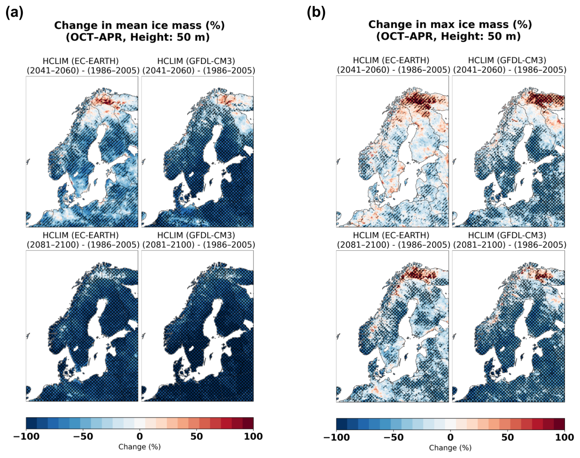
Figure 2 Relative change in (a) mean ice mass, (b) mean annual maximum ice mass at the model height of 50 m. In the upper panel, the changes in icing from the historical period to mid-century and for both model configurations (EC-EARTH and GFDL-CM3) are shown. In the lower panel, the change from the historical period to end-of-century is shown. Statistically significant areas are shown with hatching, areas marked with slash are significant by the 0.1 confidence level, while areas with backslash are significant by the FDR-corrected confidence level.

There is greater variability in the results for maximum ice masses. Figure 2b depicts the relative change in annual maximum ice masses (absolute changes are seen in Fig. A1b). With the maxima, a statistically significant increasing signal persists until end-of-century in northern Lapland, northern Norway and Kola-Peninsula in HCLIM with EC-EARTH. A similar trend is present in HCLIM with GFDL-CM3 in mid-century. The increasing trend is more pronounced for EC-EARTH, where the increase is greater than 50 % in northern Lapland and Norway for both time spans; in GFDL-CM3, the increasing trend is limited only to Kola-Peninsula by end-of-century. In other areas where increase is projected, mostly elsewhere over northern Fennoscandia or the Scandinavian mountains, the increase is not statistically significant or only significant by the 0.1 confidence level. FDR-limited significant decreasing trends are rare in HCLIM with EC-EARTH in mid-century and located mostly in western Norway (20 %–50 %); in end-of-century significant decreasing trends become more widespread and seen around the study region. According to HCLIM with GFDL-CM3, FDR-limited significant trends are projected in many parts of the southern and central parts of the domain already in mid-century and more widely by end-of-century. A clear example of differences with the projections is over western Finland, where a decreasing trend is pronounced in HCLIM with GFDL-CM3 both in mid-century and in end-of-century (50 %–100 %); the trend is also evident for absolute values (locally above −0.1 kg m⁻¹ in Fig. A1b).

Beyond the actual ice masses accumulated on structures, the duration of the presence of ice is crucial; hence, changes in icing hours were examined. Here, as explained in Sect. 2.3.1, an icing hour is described as an hour with an ice cover thickness of ≥ 2 mm in the model cylinder. Figure 3 visualizes the relative change in annual mean icing hours in the Fennoscandian area. A significant decreasing trend is prevalent in most of the study area, with a more substantial decrease in GFDL-CM3-based outputs; in southern and central Finland, a decrease of 80 %–100 % is projected by the end-of-century. For absolute changes in icing hours (Fig. A2), the largest changes are in northern parts of Finland, central and northern Sweden, and the Scandinavian mountains, where a decrease of 500–1000 h annually (20–40 d) is projected for the mid-century and close to 1000 h or even more for the end-of-century (40 d or more). This corresponds to a 10 %–50 % decrease in the mid-century; by the end-of-century, a 60 %–80 % decrease is simulated over central Sweden and southern Lapland, while northern Lapland is expected to see a 40 %–60 % decrease. Locally, some of the weakest decreasing trends in the northern and eastern parts of the domain are not statistically significant. Additionally, none of the localized increasing trends are statistically significant.

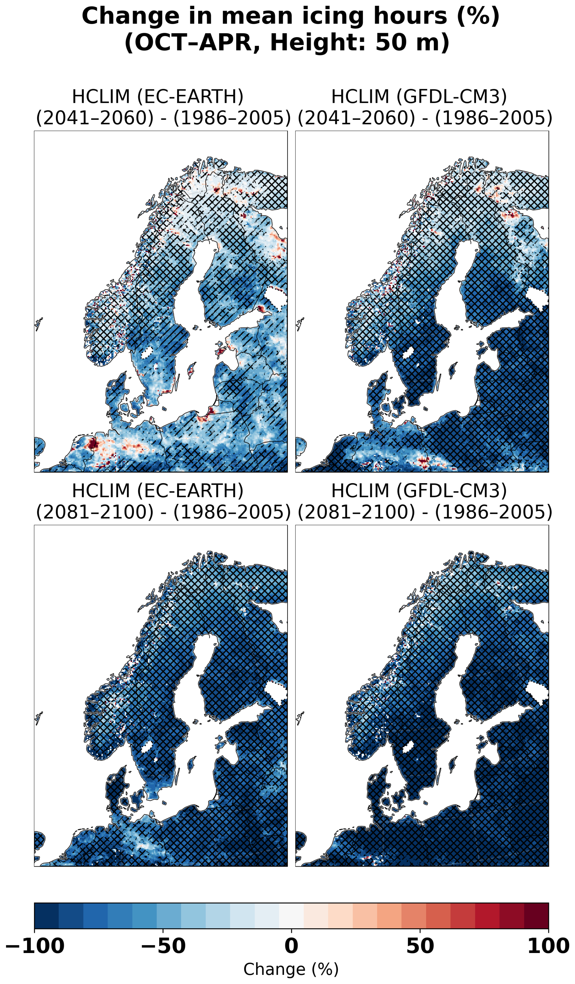
Figure 3 Relative change in annual mean icing hours at the model height of 50 m. In the upper panel, the changes in icing from the historical period to mid-century and for both model configurations (EC-EARTH and GFDL-CM3) are shown. In the lower panel, the changes from the historical period to end-of-century are shown. Statistically significant areas are shown with hatching, areas marked with slash are significant by the 0.1 confidence level, while areas with backslash are significant by the FDR-corrected confidence level.

3.2.2 Test areas 6–7: Power line perspective (50 m height)

To study changes in icing conditions in more detail, various areas were selected for further analysis. This section presents results related to ice masses, thicknesses, and icing episode durations at 50 m from two areas presented in Fig. 1; one in eastern Finland (6: Kontiolahti) and the second in northernmost Finland (7: Utsjoki). Both areas cover 66 grid points in total and they are situated in relatively low terrain (average altitudes of 110 m in Kontiolahti and 245 m in Utsjoki, Table B5). Additionally, in Sect. 2.3.1 we have outlined the methods and definitions used to derive the parameters applied here, such as an icing episode.

For Kontiolahti, results are presented in Fig. 4a–b, while Fig. 4c–d show the same for Utsjoki. In box plots (Fig. 4a and c), the evolution of regional maximum ice masses are visualized with both the annual mean and the annual maximum shown for the regional maximum of the grid points. In Kontiolahti, a decreasing trend is noticeable as the median values show a decrease across time periods with both configurations. The extremes of the distributions (whiskers) also show decreasing trend. Moreover, according to the GFDL-CM3 boundary model, the maxima of the mean distribution become smaller than the median value in the historical period for both locations; this is mostly supported by HCLIM with EC-EARTH, however, there are outliers in both locations.

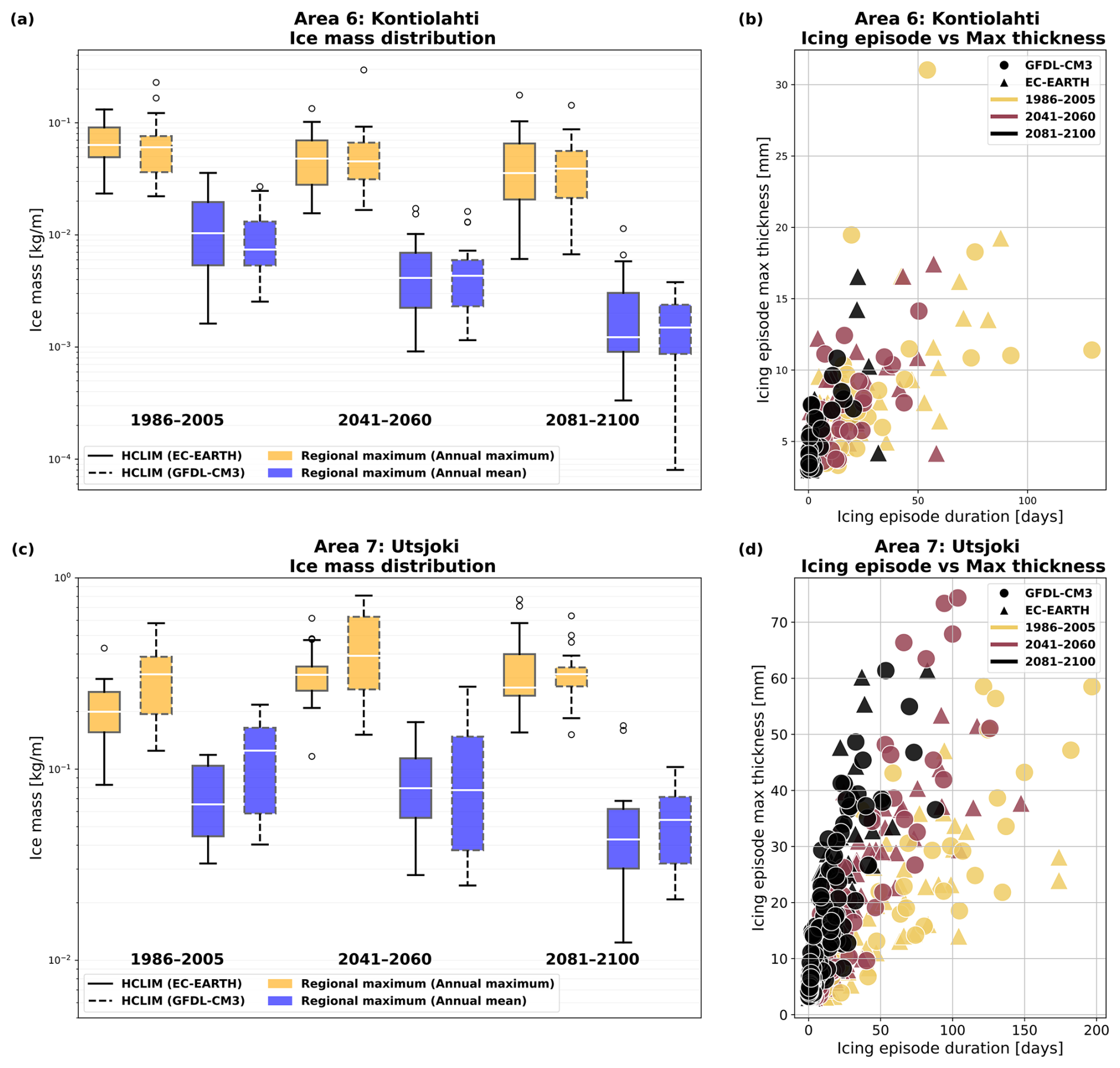
Figure 4 Regional results at the height of 50 m from Kontiolahti (a–b) and from Utsjoki (c–d). In panels (a) and (c) distributions of yearly maxima (yellow) and means (blue) are shown for the regional maxima. Boxes with solid lines are EC-EARTH and dashed lines GFDL-CM3. The white line indicates the median value while the boxes cover the interquartile range. Whiskers extend close to the extremes of the distributions, and dots cover the outliers. In panels (b) and (d) the relation of icing episode duration and maximum thickness of ice cover during the episode are shown. Triangles denote EC-EARTH and circles GFDL-CM3 while historical values are shown in yellow, mid-century in red and end-of-century in black. Icing episode denotes to the period when ice cover thickness ≥ 2 mm.

With Utsjoki, the results exhibit greater variability. GFDL-CM3 shows a decrease in the median values and interquartile range across the time periods, while EC-EARTH projects slight increase in the mid-century turning towards decreasing in the end-of-century. Smallest mean values (whiskers) are projected in both models in the end-of-century period, while the largest mean values (if excluding outliers) are shown for mid-century. Generally, the mean values are smaller in EC-EARTH than in GFDL-CM3 in Utsjoki, while the situation is somewhat opposite in Kontiolahti.

While decreasing trends can be distinguished in Kontiolahti for annual means, the signal is less clear with annual maxima. The median values decrease slightly when comparing future periods with the historical period. Between future periods, the trend is neutral. In end-of-century, there is indication of increased variability caused by a decrease in the minima of the distributions. In Utsjoki, both model configurations show an increase in mid-century and, for EC-EARTH, the maxima of the distributions increase until the end-of-century. Thus, while mean ice masses are expected to mostly decrease (as discussed in Sect. 3.2.1), the potential for larger ice masses remains.

Changes in the relationship between the maximum thickness of the ice cover during an icing episode and the duration of such an episode are depicted for both model configurations in Fig. 4b and d. There are some regional differences in the scatter plots; for Kontiolahti (Fig. 4b), a shift toward shorter episodes and thinner ice covers is expected, while in Utsjoki, thick covers persist even with decreasing episode lengths (Fig. 4d). In Kontiolahti, icing episode lengths of 0–40 d are most common with a maximum thickness of 3–15 mm, with the largest thicknesses of 20–35 mm occurring when icing episode lengths exceed 20 d. HCLIM with EC-EARTH suggests slightly more potential for thicker covers (10–35 mm) and longer episodes (over 40 d) than HCLIM with GFDL-CM3. In Utsjoki, maximum thicknesses are generally around 40–60 mm across boundary models and time periods. In mid-century, there is indication of an increased chance of thicknesses of more than 60 mm in HCLIM with GFDL-CM3.

3.2.3 Test areas 1–5: Wind power perspective (50–400 m height)

In this section, results from all the five output heights (50, 100, 200, 300, and 400 m) are investigated in the case study area of Kauhajoki located in western Finland along with four additional areas around Fennoscandia. These areas correspond to areas 1–5 presented in Fig. 1, and they coincide with existing or planned wind park locations. All areas cover 42 grid points in total, and while areas 1–3 are in relatively low terrain (average altitudes above sea level in HCLIM data are under 200 m), areas 4–5 are situated in higher terrain with average altitudes of around 550–600 m, with the highest simulated altitude in area 4 (922 m, Table B5). Consequently, here an icing hour is described differently from Sect. 3.2 to better align with wind power standards (≥ 10 g m⁻¹ of ice present in the cylinder). However, an important factor here is to note that the model output was calculated for a cylinder of diameter of 3 cm, which is more suited for transmission lines than for wind turbines.

For Kauhajoki, yearly icing hours at heights 50–400 m are presented in Fig. 5, with distributions presented for each time period. It is evident that the number of icing hours decreases with time at each height and for both boundary models. For HCLIM with GFDL-CM3 (Fig. 5b), at upper heights of 200–400 m, the mean icing hour values in the mid-century period align with or are smaller than the minimum values in the historical period, while at the end-of-century, the simulated maximum hours align with or are smaller than the minimum values in history. With EC-EARTH (Fig. 5a), the distributions in future periods cover a wider spectrum, although with a similar decreasing trend. At lower heights of 50–100 m, there are individual years with more than 1000 h of significant ice present in the historical period, but none forecasted for the end-of-century. If we compare the heights of 300 and 100 m, the mid-century mean in 300 m is greater than the historical mean in 100 m for both configurations; an interesting point to consider, as wind turbine heights have increased with time. A similar plot of the distributions of icing episode durations is presented in Fig. A4; the decrease in durations for this location is strongest in HCLIM with GFDL-CM3.

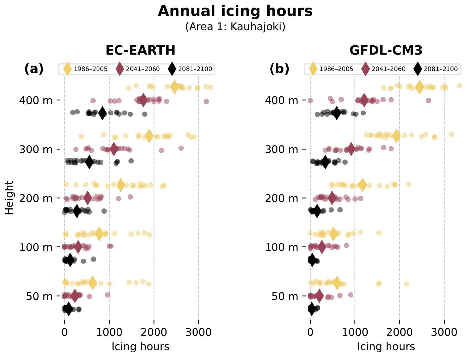
Figure 5 The distribution of annual icing hours at different heights (ranging from 50 to 400 m) averaged over a box in area 1 (Kauhajoki) with (a) EC-EARTH (b) GFDL-CM3 as the boundary climate model. Yellow dots denote the historical period, red the mid-century and black the end-of-century with vertical line indicating the conditional mean value.

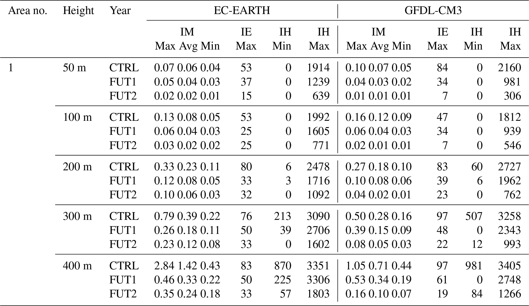
In Table 2, results for Kauhajoki can be found in numerical format, including the maximum and minimum icing hours for each height and time period. In addition, the maximum icing episode length (when averaged over the area) and the range of the 99th quantile of ice masses (maximum-average-minimum in the area) for each period are presented. As noted before, with icing hours and icing episodes, the trend is towards decreasing amounts; according to HCLIM (GFDL-CM3), in the future, a year without icing could occur even at 400 m height in Kauhajoki. Also notable is the decrease in the maximum icing episode lengths; from 50–100 d to around 5–35 d by the end-of-century depending on the boundary model and height. For the ice masses, the signal is also decreasing, and with HCLIM (GFDL-CM3), the average 99th quantile is 0.1 kg m⁻¹ even at 400 m by the end-of-century.

Table 2 Numerical results for Kauhajoki (area 1, western Finland). CTRL is for the historical period (1986–2005), FUT1 is the mid-century (2041–2060) and FUT2 the end-of-century (2081–2100). For each time period and GCM (EC-EARTH and GFDL-CM3, respectively), six numerical values are given. IM (Max Avg Min) is for the regional maximum, average and minimum of the 99th quantile of ice mass (in kg m⁻¹), first determined for each grid point separately in the area. IE Max denotes the maximum ice episode duration (days) taken from the average of the area and IH (Min & Max) denote the minimum and maximum icing hour amounts (hours), taken also from the regional average.

In Tables B1–B4, results are collected from additional study areas. For Pello (area 3 in northwestern Finland, Table B2), results indicate mixed signals for the 99th quantile ice mass at the height of 50 m with decreasing trends from 100 m upwards (from highest values of 1–3 kg m⁻¹ in the area in the historical period to 0.4–2 kg m⁻¹ in future periods). For the rest of the areas, trends in both ice masses and icing durations are decreasing. In area 2 (Haapajärvi, Table B1), by the end-of-century, the 99th quantiles become dominantly smaller than 1 kg m⁻¹ across both models and all heights, while the maximum episode durations change from 70–175 d to around 15–50 d. For area 4 (around Narvik, Norway; Table B3), the maxima of the 99th quantile ice masses range from 20 to 40 kg m⁻¹ in history and from 7 to 20 kg m⁻¹ at the end-of-century across heights and both model configurations. For Rutan (area 5 in central Sweden, Table B4), maximum durations decrease from over 100 d to under 100 d starting from mid-century, while the 99th quantile loads are reduced by more than half in HCLIM with GFDL-CM3 (less with EC-EARTH).

3.3 Future changes in HCLIM output parameters (50 m height)

The meteorological input parameters from HCLIM to the rime ice model are temperature, cloud liquid water content, and wind speed. Hence, changes in icing are a consequence of changes in these three parameters, and in this section, the simulated changes of these parameters at the height of 50 m are investigated.

3.3.1 Temperature

Ice formation takes place at freezing temperatures; therefore, it is important to consider how often freezing conditions occur. The critical threshold temperature between icing and melting in the rime ice model is set to 0 °C, above which water remains liquid or the existing ice melts. In reality, this can vary depending on the type of icing and other meteorological conditions, such as the presence of ice nucleation particles (International Organization for Standardization, 2017). In contrast, at sufficiently low temperatures, around and lower than −20 °C, ice accumulation from supercooled liquid droplets is limited, as the air can only hold a small amount of liquid water (Westbrook and Illingworth, 2011).

Exploring changes in the occurrence of the critical temperature threshold is important, as it dictates the effect of temperature on icing. In Fig. 6a, the mean temperatures of a typical icing season (October–April) at 50 m are shown for the historical period and the two future periods (2041–2060, 2081–2100). The boundary model in the upper panel is EC-EARTH, and in the lower panel, GFDL-CM3. It is evident that the mean temperature in the historical period is widely below 0 °C from the northern to central parts of the domain. By the end-of-century, the mean temperature is projected to be below zero only in northern Lapland and over Scandinavian mountains corresponding to the strongly warming emission scenario RCP 8.5.

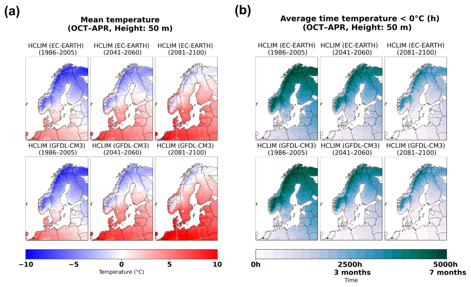
Figure 6 Temperature in 50 m. In panel (a) the mean temperature (50 m) of October–April period is shown, while panel (b) shows the average time that temperature is below zero (October to April). In both panels (a) and (b), the historical period is shown in the left panel, the mid-century in the middle panel, and the end-of-century period in the right panel. The upper row is for HCLIM with EC-EARTH and the bottom row for HCLIM with GFDL-CM3.

An important factor to consider is how much time is spent under freezing conditions even in a highly warming future. Figure 6b shows the average hours spent below 0 °C at the height of 50 m in historical and future periods. The time spent in freezing conditions decreases everywhere in the domain. Excluding southern Sweden and some of the coastal regions in Norway, Fennoscandia experiences around 4–7 months of freezing temperatures in the historical period. For the mid-century, this drops down to 2–6 months, except for mountainous regions. However, for the end-of-century, southern and central Fennoscandia fall under an average of 0–2 months, northern parts to 2–4 months, and the highest altitudes on average to 4–6 months of freezing temperatures. Some areas in the southern part of the domain, such as the south-western coast of Finland, southernmost Sweden, coastal regions of Norway and Baltic states, and Denmark, may experience close to zero months of freezing conditions at the end-of-century.

The effect of the strong warming is especially present in the mean changes (ice mass and icing hours), for which widespread decreases are projected already in mid-century. For the mean parameters, the icing across the whole winter season counts, and if the winter period becomes noticeably short, this will be reflected in the mean parameters. As an exception, the northernmost areas can experience, in the mid-century, a long enough cold season but with less time spent in very cold temperatures, so that local increase is projected. With ice mass maxima, a similar effect is present. For the largest ice buildups, consecutive time in freezing temperatures is needed. In the northernmost areas, the projected future icing episodes are still long enough for significant ice buildup to occur, while the episodes themselves will happen in warmer and moister conditions. This allows for larger masses than in the historical period.

3.3.2 Cloud liquid water content and wind speed

The amount of cloud liquid water content in the atmosphere defines how much ice is possible to accumulate from in-cloud icing if other meteorological conditions are favorable. The function of wind in relation to atmospheric icing is then to transport liquid droplets to the surface of an object where ice may form. If the wind speed is high, transportation is more efficient compared to situations with calmer winds. The icing model used in this study assumes a freely rotating cylinder, thus, wind direction is not considered.

The relative change in the mean CLWC values at the model height of 50 m can be seen in Fig. 7a, while the relative changes in mean wind speed are shown in Fig. 7b. An increasing trend (dominating red colors) is present in most of Fennoscandia for both mid-century and end-of-century for cloud liquid water content, applying particularly for HCLIM with EC-EARTH. With mean wind speed, only minor changes are predicted, at least in HCLIM with EC-EARTH; HCLIM (GFDL-CM3) projects increase of about 10 %–15 % in cold season wind speeds in the southern parts of the domain in end-of-century. Oppositely, GFDL-CM3 simulates there a slight decreasing trend in mean CLWC, by the end-of-century also in most of the Finnish and Swedish coastal areas. In EC-EARTH, a similar pattern is present on the western coast of Norway, while HCLIM with GFDL-CM3 predicts mostly an increasing trend. The absolute changes in the mean CLWC are shown in Fig. A3a and for wind speeds in Fig. A3b. The strongest absolute increase in mean CLWC can be seen at higher altitudes, with an increase of 0.02 g m⁻³, while the absolute increase in mean wind speed in GFDL-CM3 is around 0.5–1 m s⁻¹.

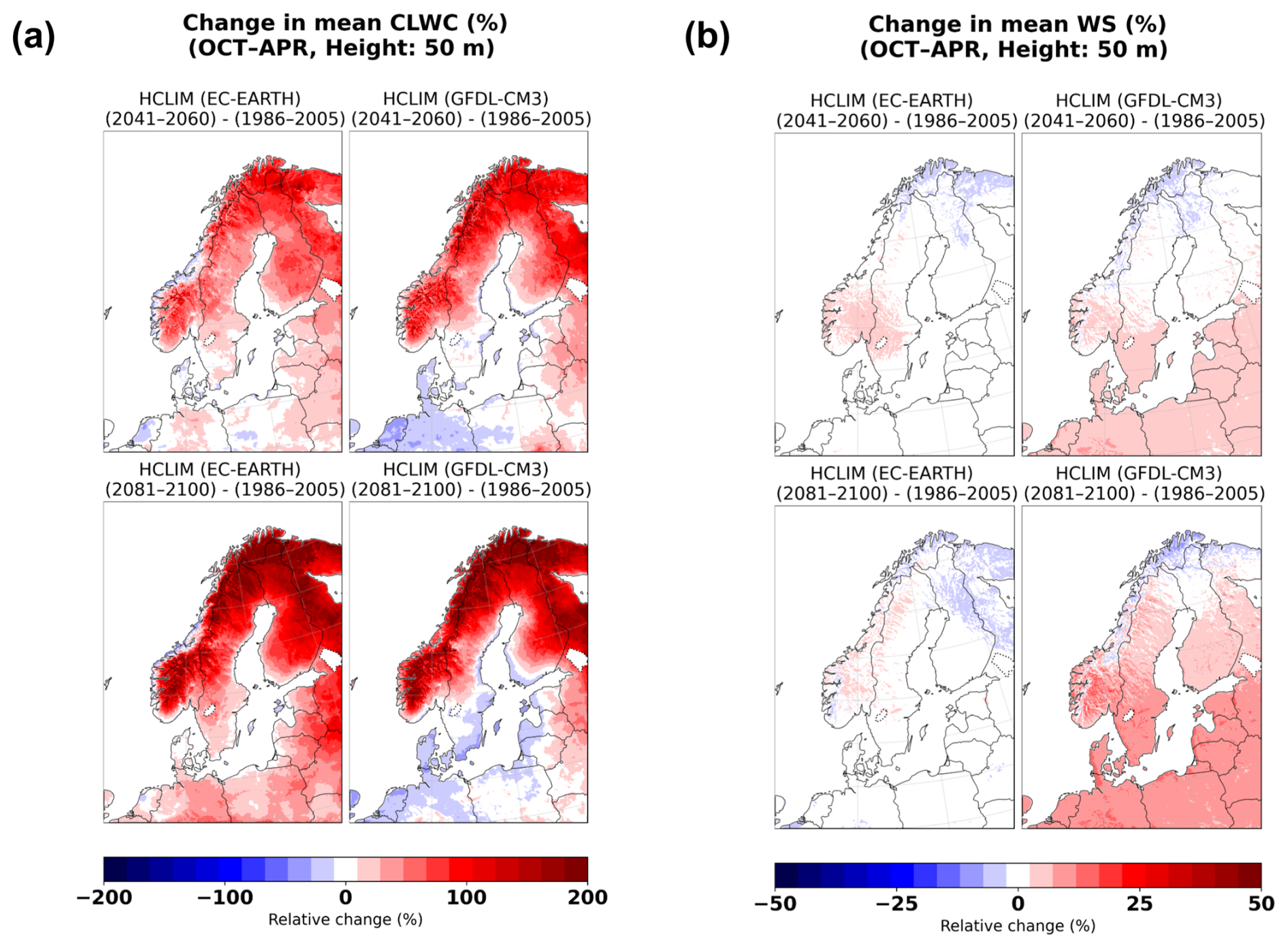
Figure 7 The relative change in (a) mean cloud liquid water content, (b) mean wind speed at model height of 50 m for both GCMs (EC-EARTH in the left column, GFDL-CM3 in the right column). The upper rows compare the mid-century (2041–2060) with the historical period (1986–2005), while the bottom rows compare the end-of-century (2081–2100) with history.

This widely increasing trend in CLWC aligns with a warming climate, as warmer air can hold more moisture and, thus, liquid water in an atmospheric layer. However, mostly decreasing icing trends are projected for northern Europe, which indicates that in most areas, the loss of time spent under freezing temperatures dominates the effect on icing. Temperature's dominating effect is supported by the changes in wind speed, as either little change (HCLIM with EC-EARTH) or slight increase (HCLIM with GFDL-CM3) is projected. In northernmost areas, the strong increase in mean CLWC can help to obtain larger maxima. In western and southern parts of Finland and southern Sweden, however, the slightly decreasing trend in CLWC in HCLIM with GFDL-CM3 can add to the projected stronger warming and explain the robust decreasing signal in annual ice mass maxima in these regions in HCLIM with GFDL-CM3.

4 Discussion

Based on our projections, in-cloud icing decreases in most areas across Fennoscandia. This reduction is expected in both the amount of ice and the duration of icing periods. The predicted trends are stronger with HCLIM (GFDL-CM3), as of the two GCMs, it has a warmer response to climate change. We suggest that the main driver for the decrease is the warming trend in temperatures. Although the warmer atmosphere allows for a higher moisture content, icing does not occur when temperatures are above 0 °C. The increasing trend in annual maxima over some of the northern regions could be explained by the increase of CLWC over regions where freezing temperatures persist, but, on the other hand, the temperatures are not too cold, allowing water to stay in liquid form. A similar, but less certain, trend is present with mean ice mass in mid-century; however, with mean values, the strong warming across the study region plays an even more crucial role.

Our results primarily indicate reductions in icing-related hazards affecting energy infrastructure. Icing frequencies (counted both in annual icing hours and in episode durations) and mean icing see a widespread reduction, which would mean less and shorter disruptions to wind power production and energy transmission and less wear on the energy infrastructure. However, our results from a test area related to wind production suggests that as wind turbine heights increase, significant icing may still occur at levels similar to or even greater than those observed today. This is based on comparing icing at the heights of 300 and 100 m, where on average, more icing hours are projected in mid-century in 300 m compared to 100 m in the historical period.

For transmission lines, the largest icing events should also be considered as those can cause significant hazards. The largest masses are encountered in higher altitudes; across the Scandinavian mountains, mixed signals are projected. Much of the southern and central regions (especially western Norway) see a significant decrease. An increase is locally projected, however, with limited certainty in the signal. Moreover, as discussed previously, increase in annual maxima is projected in northern regions. When inspecting the distribution of the maxima in a test area in northernmost Finland, even the lower ends of the simulated maxima are larger in end-of-century than in the historical period in both model configurations. This highlights the influence that increased liquid water content can have in a warmer climate. In another test area in eastern Finland, the maxima distributions exhibit greater variability toward the end-of-century, driven by a decrease in their lowest values. This stems from the pronounced projected warming, which also results in decreased icing episode durations in both areas.

Our results add to previous studies on icing changes in Fennoscandian region conducted by Iversen et al. (2023) and Lutz et al. (2019). Our research expands the regions where future icing has been studied in northern Europe and also extends the analysis for multiple tropospheric heights and for a higher horizontal resolution. In the research of Iversen et al. (2023), the projections for 10-year rime ice loads based on two model configurations showed different change signals across Scandinavian mountains with one showing increasing amounts towards the end of the century while wide decrease was projected by the configuration with stronger warming. Our results, although for annual maxima, correspond better with the warmer configuration. This is understandable as RCP 8.5-based warming is rather strong even in the colder of our two configurations, HCLIM with EC-EARTH; the projections of Iversen et al. (2023) cover RCPs ranging from 2.6 to 7.0. Their projections also suggest a possibility for increase in parts of the northernmost regions, but with less certainty than in our study. Our research then contributes to pinpoint northern regions of Fennoscandia as a possible region of increased icing hazards if strong warming occurs.

However, Lutz et al. (2019) used the EURO-CORDEX ensemble with RCP 8.5 pathway, and in their ensemble mean for end of the century, increase in annual maxima is projected in a wider area than in our research. It can be noted that an increase is shown for all of the ensemble members in northern regions, while for example in central Finland, the signal has a lot of variation. This highlights that icing is a complex phenomenon, as ice formation depends on numerous meteorological parameters, making its modeling, prediction, and observation challenging.

For our simulations, the largest uncertainties have to do with the absolute values as explained in Sect. 3.1. For comparison, Iversen et al. (2023) reported 10-year ice loads at the surface of 0–5 kg m⁻¹, locally more, in lowlands, and up to at least 30 kg m⁻¹ in the Scandinavian mountains. Our projections showed values around 0–2 kg m⁻¹ in lowlands at the lowest height of 50 m and in the Scandinavian mountains up to at least 20–30 kg m⁻¹. Lutz et al. (2019) saw a huge variation in ice masses corresponding to the differences in calculated CLWC; their simulated ensemble mean ice loads are of magnitude 20–40 kg m⁻¹ in many parts of Finland and Sweden, which seems rather large taking into account that this range aligns more with values reported for higher terrain (Nygaard et al., 2022, 2014). This underlines again the complexity of icing simulations, where uncertainties especially with modelled CLWC affects the icing simulations. Overall, our absolute values carry uncertainty, especially in lower terrain.

Using high-resolution data from multiple heights hinders an ensemble approach, which is a big limitation of our study. For example, the RCP 8.5 pathway scenario used in this study is a high emission scenario, leading to substantial warming. Consequently, the predicted reduction in icing might be overestimated with current understanding suggesting that we are moving towards the RCP 4.5 scenario; however, future decades could bring changes depending on the actions taken. An additional uncertainty in our results is that they are based on the phase 5 Coupled Model Intercomparison Project (CMIP5) projections which are suggested to have too little spread in their response to changes in the Atlantic meridional overturning circulation (AMOC) (Liu et al., 2017); the collapse of which would have major consequences in the regional climate of northern Europe (van Westen et al., 2024). Moreover, from purely power transmission line perspective, including wet snow simulations could have offered additional value, but it was outside the scope of this study.

5 Conclusions

The objective of this study was to assess the simulated changes in rime ice formation during in-cloud icing episodes across the Fennoscandian region. We utilized high-resolution climate model outputs driven by two GCMs (HCLIM with EC-EARTH and GFDL-CM3) under the highly warming RCP 8.5 scenario. In our study, the focus was both on a model height close to the surface (50 m) to investigate icing on power lines, and on four additional heights (100–400 m), as atmospheric icing across the boundary layer impacts wind energy production in northern latitudes. Results covered both the whole Fennoscandian area (50 m, power transmission lines) and specific areas (50–400 m, both transmission lines and wind energy).

Both GCMs agree that, in general, there is a significant decreasing trend in mean rime ice conditions at the height of 50 m over most of Fennoscandia by the end-of-century, and, similarly, the time spent under icing conditions is predicted to generally decrease in the Fennoscandian region. A similar effect is suggested for the heights of 100–400 m in the five wind power specific test areas, although with increasing turbine heights, icing risks similar to those observed today may still be encountered. In the test areas concerning power transmission lines, the relationship between the maximum thickness obtained during an icing episode and the episode duration was examined. In eastern Finland, both the thickness and the durations are generally expected to decrease, while in northernmost Finland, large maxima are expected even by the end-of-century, but reached with shorter episode lengths.

In general, the estimated response of annual ice mass maxima to climate change shows more variation than that of mean ice masses. While southern and central Fennoscandia are predicted to experience largely a decreasing trend, over parts of northern Fennoscandia and Scandinavian mountains, an increasing trend remains until the end-of-century. In HCLIM with GFDL-CM3, this response is more restricted than in HCLIM with EC-EARTH.

Although our results indicate a future where icing events become rarer, atmospheric icing as a phenomenon will not disappear, not even at the lowest near-surface layers. More research in high horizontal and vertical resolution is needed that uses an ensemble approach with both regional climate models and pathway scenarios. Subsequently, a better understanding of future icing conditions can be achieved to prepare and design the energy infrastructure to be sustainable.

Appendix A: Figures

Figure A1 Same as in Fig. 2 but for absolute ice masses.

Figure A2 Same as in Fig. 3 but for absolute change in yearly icing hours.

Figure A3 Same as in Fig. 7 but for absolute changes in (a) mean liquid water content, (b) mean wind speed at the height of 50 m.

Figure A4 Same as in Fig. 5 but for icing episode durations at different heights (from 50 to 400 m) with (a) EC-EARTH (b) GFDL-CM3 as the boundary climate model.

Appendix B: Tables

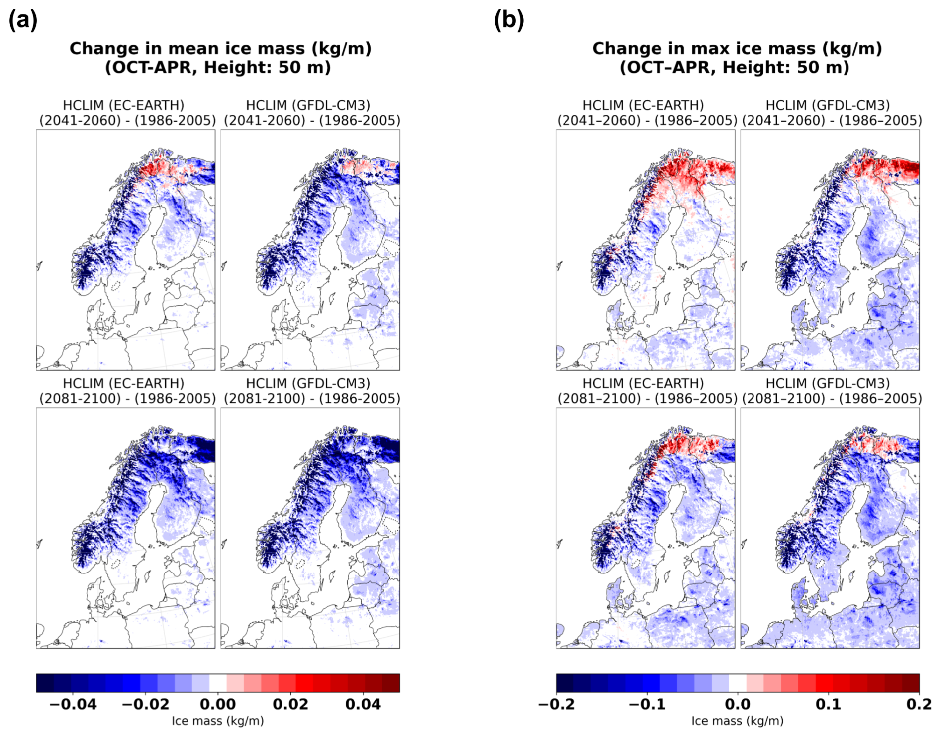
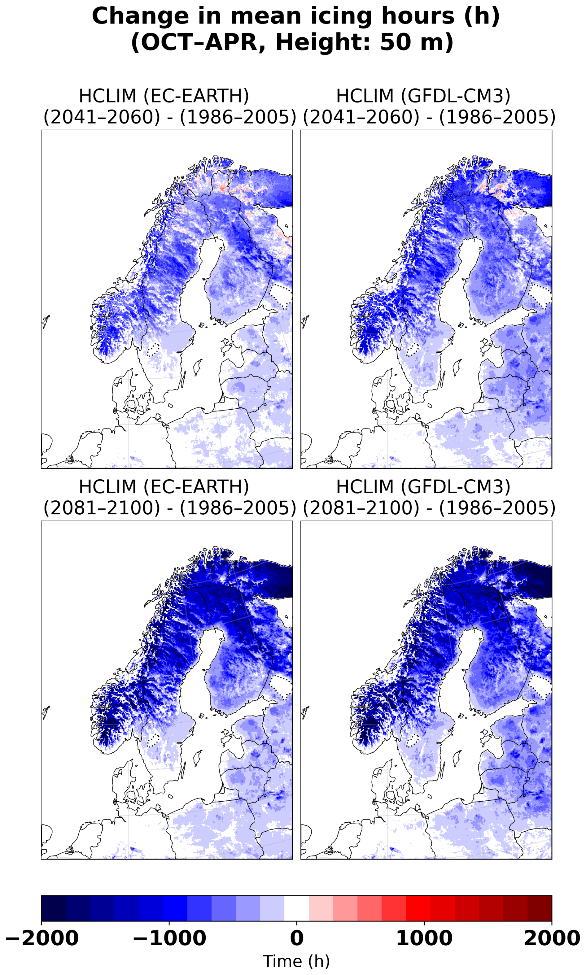
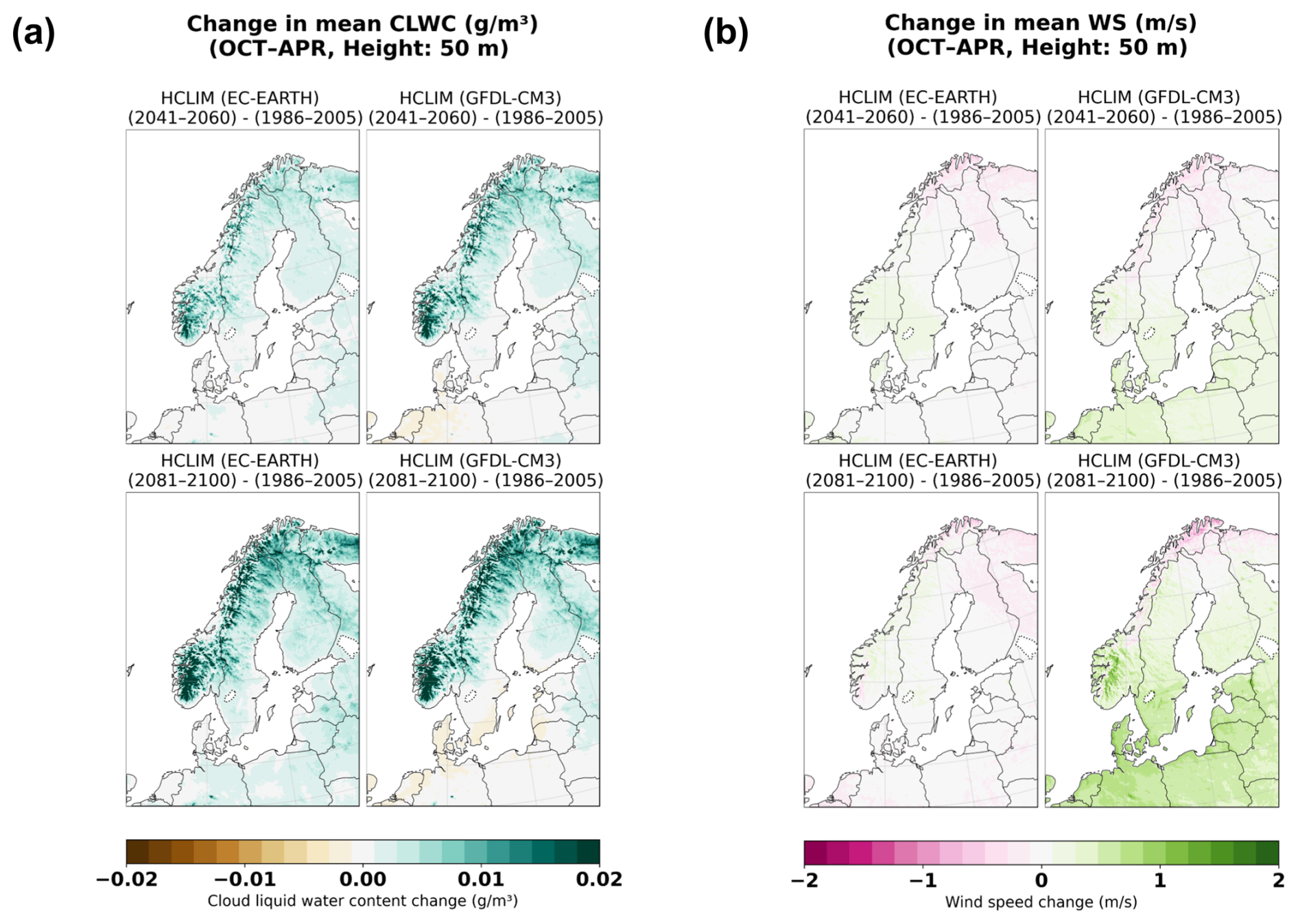
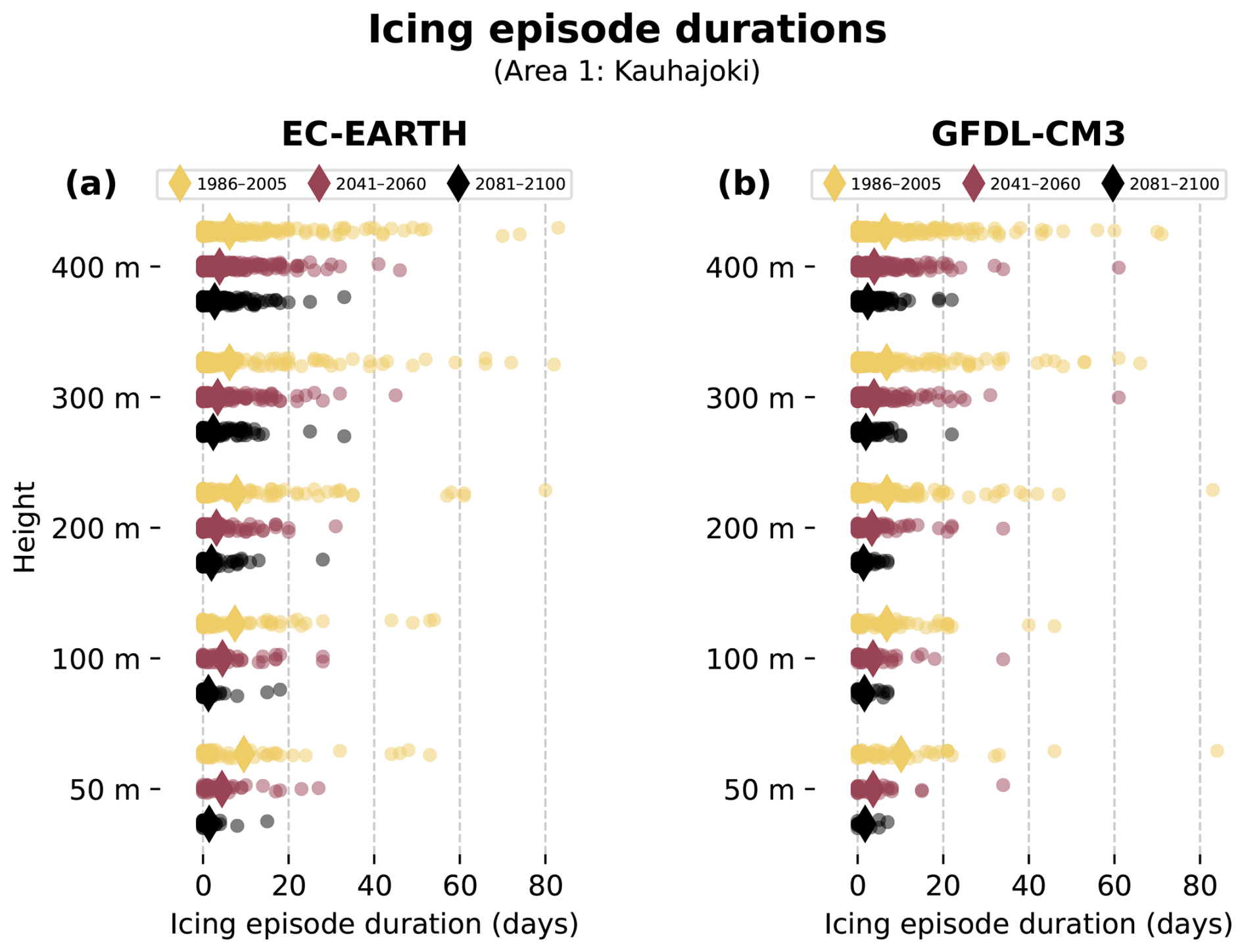
Table B1 Numerical results for Haapajärvi (area 2, northern Finland). CTRL is for the historical period (1986–2005), FUT1 is the mid-century (2041–2060) and FUT2 the end-of-century (2081–2100). For each time period and GCM (EC-EARTH and GFDL-CM3, respectively), six numerical values are given. IM (Max Avg Min) is for the regional maximum, average and minimum of the 99th quantile of ice mass (in kg m⁻¹). IE Max denotes the maximum ice episode duration (days) taken from the average of the area and IH (Min & Max) denote the minimum and maximum icing hour amounts (hours), taken also from the regional average.

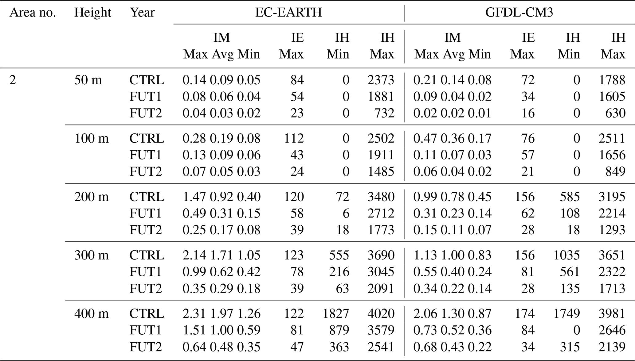
Table B2 Numerical results for Pello (area 3, Finnish Lapland). CTRL is for the historical period (1986–2005), FUT1 is the mid-century (2041–2060) and FUT2 the end-of-century (2081–2100). For each time period and GCM (EC-EARTH and GFDL-CM3, respectively), six numerical values are given. IM (Max Avg Min) is for the regional maximum, average and minimum of the 99th quantile of ice mass (in kg m⁻¹). IE Max denotes the maximum ice episode duration (days) taken from the average of the area and IH (Min & Max) denote the minimum and maximum icing hour amounts (hours), taken also from the regional average.

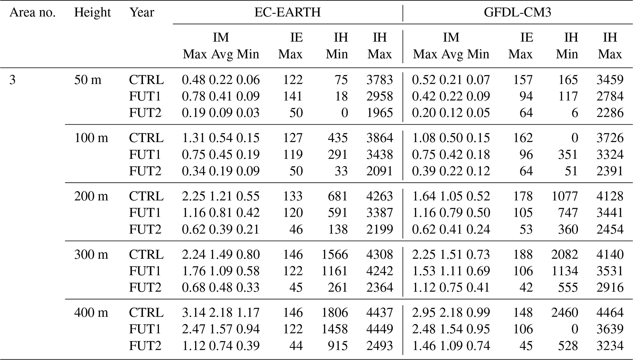
Table B3 Numerical results for Narvik (area 4, northern Norway). CTRL is for the historical period (1986–2005), FUT1 is the mid-century (2041–2060) and FUT2 the end-of-century (2081–2100). For each time period and GCM (EC-EARTH and GFDL-CM3, respectively), six numerical values are given. IM (Max Avg Min) is for the regional maximum, average and minimum of the 99th quantile of ice mass (in kg m⁻¹). IE Max denotes the maximum ice episode duration (days) taken from the average of the area and IH (Min & Max) denote the minimum and maximum icing hour amounts (hours), taken also from the regional average.

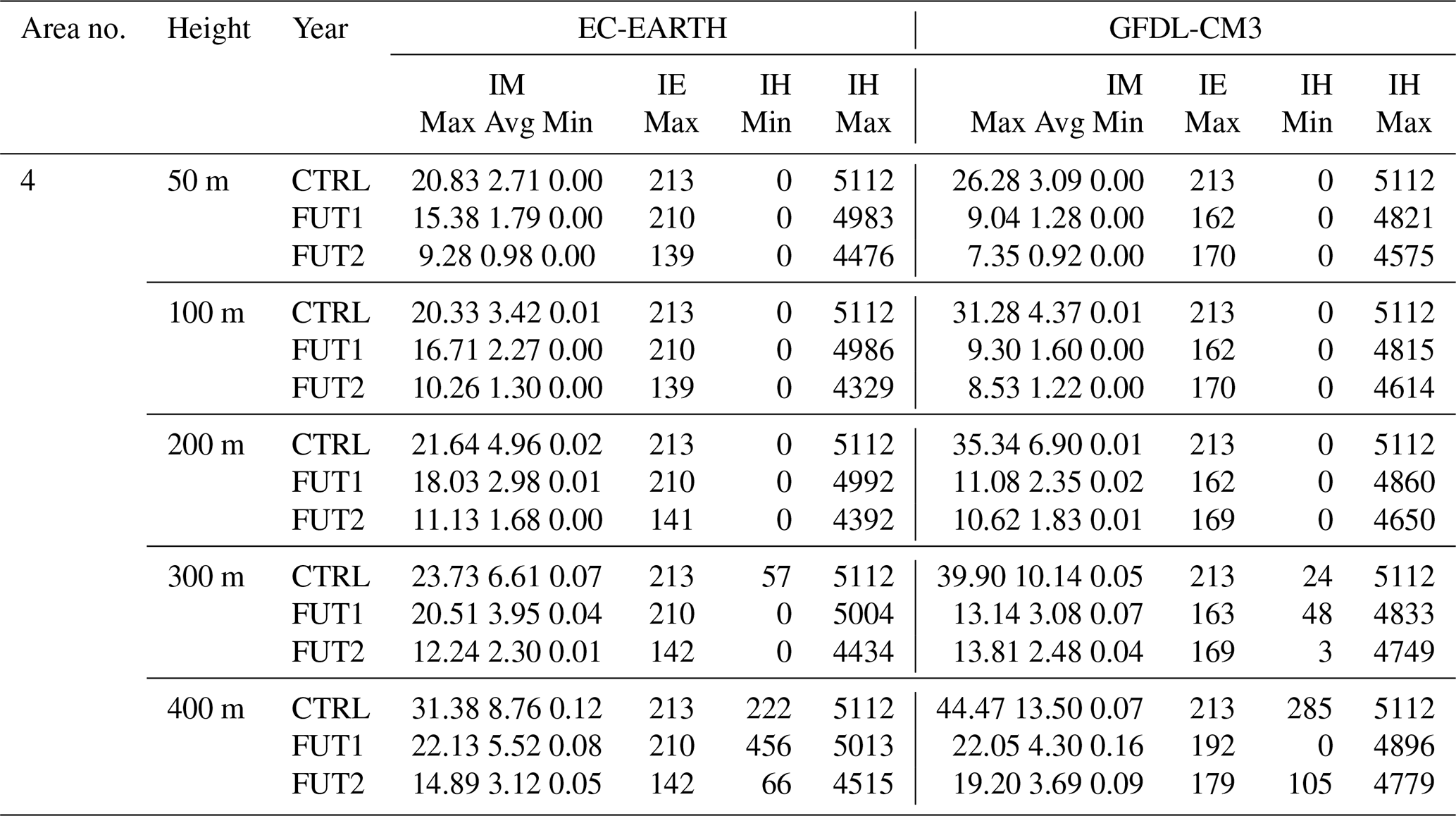
Table B4 Numerical results for Rutan (area 5, central Sweden). CTRL is for the historical period (1986–2005), FUT1 is the mid-century (2041–2060) and FUT2 the end-of-century (2081–2100). For each time period and GCM (EC-EARTH and GFDL-CM3, respectively), six numerical values are given. IM (Max Avg Min) is for the regional maximum, average and minimum of the 99th quantile of ice mass (in kg m⁻¹). IE Max denotes the maximum ice episode duration (days) taken from the average of the area and IH (Min & Max) denote the minimum and maximum icing hour amounts (hours), taken also from the regional average.

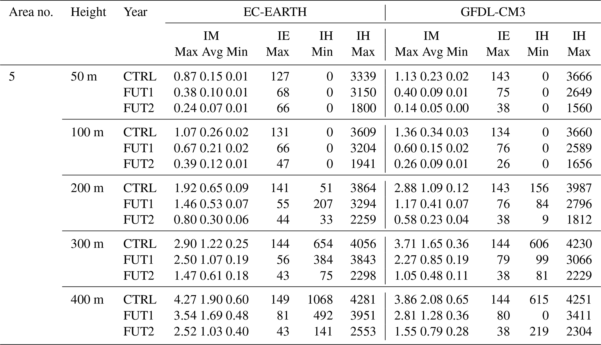
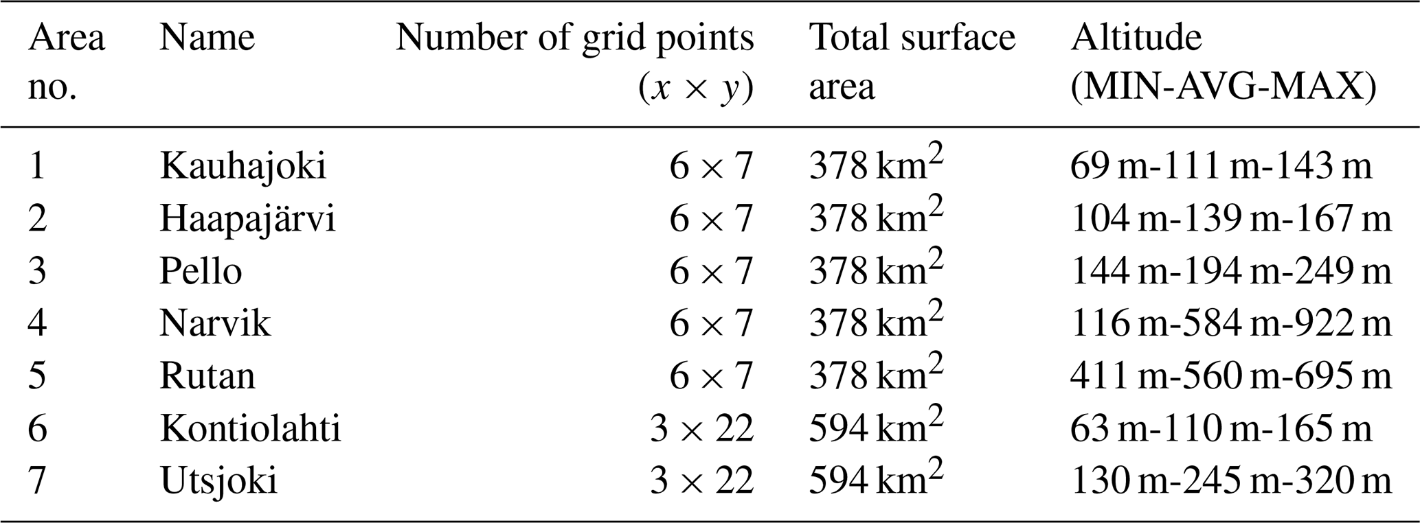
Table B5 Supplementary information is shown for areas 1–7. This includes the number of grid points and, thus, the total surface area coverage of each area, and the minimum, average and maximum surface altitudes above sea level (in HCLIM model data). The locations of the areas can be found in Fig. 1.