Assessing sea level rise and extreme events along the China–Europe Sea Route

The Intergovernmental Panel on Climate Change (IPCC) Sixth Assessment Report highlights the accelerating rise of global mean sea level (GMSL), with trends surpassing historical rates observed over the past two millennia. The China–Europe Sea Route (CESR), a region of strategic importance for international trade, is particularly vulnerable to sea level changes and extreme events. This study integrates data from satellite altimetry, tide gauge records, and a global hydrodynamic model to assess absolute and relative sea level variations, as well as extreme sea level events, across eight CESR sub-regions over the period 1993–2023.

Statistically significant mean sea level trends confirm systematic decadal variability across regions. Notably, the East China Sea, Yellow Sea and Bohai Sea show a decadal trend slowdown in the second (2003–2013) and third decade (2013–2023) with respect to the first one (1993–2003).

Signals of enhanced regional mean SLA trends are observed in the North Indian Ocean, while Pacific sub-regions exhibit pronounced decadal variability. Discrepancies between tide gauge and satellite altimetry in specific areas were attributed to land subsidence and inherent limitations of coastal altimetry.

A global hydrodynamic model provided estimates of return periods for extreme sea levels, identifying high-risk zones such as the Bay of Bengal and the South China Sea. However, challenges remain in capturing cyclone impacts, emphasizing the need for continued improvements in modeling frameworks for extreme sea level assessment.

By highlighting the importance of localized, data-driven approaches and continuous monitoring, the findings contribute to advancing climate resilience and informing risk mitigation strategies in this globally significant region.

1 Introduction

The Intergovernmental Panel for Climate Change (IPCC) Sixth Assessment Report (AR6), published in 2021, revealed unprecedented changes in the global climate system over the past two centuries (1850–2020) (IPCC, 2021). During this period, significant transformations have occurred in heat, water, and ice dynamics across various climate compartments. Among these changes, the global mean sea level (GMSL) rise stands out as a critical indicator, reflecting the interplay of complex climate processes. Since the mid-19th century, the GMSL has accelerated beyond the average rate observed over the past two millennia. Between 1901 and 2018, the GMSL rose by 0.20 m, with the rate increasing from 1.3 mm yr⁻¹ (1901–1971) to 3.7 mm yr⁻¹ (2006–2018). Satellite altimetry data further confirm this acceleration, estimating it at 0.084±0.025 mm yr⁻² between 1993 and 2018 (Nerem et al., 2018).

The primary drivers of GMSL change include the melting of polar ice sheets, land glaciers, and ocean thermal expansion. Notably, the Antarctic ice sheet mass loss tripled and the Greenland ice sheet mass loss doubled between the periods 1997–2006 and 2007–2016 (Nerem et al., 2018). Interannual variability in the water cycle can temporarily slow the trend of mean sea level rise, as observed in the global ocean from 2003 to 2011 (Cazenave et al., 2014) and in the Mediterranean Sea between 2013 and 2022 (Borile et al., 2025). These findings highlight the influence of short-term climate variability on sea level trends, which is not limited to the global scale, but also affects regional seas and localized oceanic areas. Additionally, regional sea level changes are shaped by local ocean circulation patterns, underlining the need for detailed studies of regional and coastal dynamics (Ezer et al., 2013; Pinardi et al., 2014; Dangendorf et al., 2021).

Beyond the GMSL rise, pronounced regional differences have been documented over recent decades, driven by a combination of steric effects, changes in ocean circulation, atmospheric forcing, and mass redistribution (Cazenave et al., 2014; Dangendorf et al., 2021). Along the China–Europe Sea Route (CESR), several regional studies have reported heterogeneous long-term sea level trends and accelerations, particularly in the North Indian Ocean and western Pacific, where monsoon variability, wind-driven circulation, and large-scale climate modes play a dominant role (Han et al., 2010; Huang et al., 2024).

Sea level variability in the CESR region may also be influenced by major regional circulation features, such as the Arabian Sea circulation and Somali Current, the East India Coastal Current, the Kuroshio system in the East China Sea, the Yellow Sea circulation, and the Indonesian Throughflow, which modulate regional mass transport and sea level variability (Han et al., 2010; Sprintall et al., 2014).

Extreme sea levels also exhibit strong spatial variability across the region, with storm surges and tropical-cyclone-induced extremes representing the primary drivers in areas such as the Bay of Bengal, the Arabian Sea, and the western North Pacific (Dube et al., 2009; Needham et al., 2015). Recent modelling and observational studies further indicate that changes in mean sea level and extremes may not evolve uniformly, underscoring the importance of jointly assessing long-term trends and extreme events (Tebaldi et al., 2021; Muis et al., 2016; Wahl et al., 2017; Dullaart et al., 2021).

Despite these advances, most existing studies remain focused on individual basins or specific coastal regions. As a result, a consistent and integrated assessment of mean sea level change and extreme sea levels across the entire CESR is still lacking. The present study addresses this gap by combining data from multi-mission satellite altimetry, tide gauge observations, and a global hydrodynamic model within a unified framework.

The IPCC WG1 report identified the North Indian Ocean as a region which experienced sea level rise faster than the global average, leading to coastal area loss and shoreline retreat. This region, encompassing the CESR, is of particular interest due to its importance for international trade. However, capturing the full complexity of regional sea level changes in such areas requires high-resolution, locally refined datasets that go beyond the scope of global assessments.

Efforts to monitor sea level trends on regional and global scales have been bolstered by initiatives such as the Copernicus Marine Service (CMEMS). Since 2016, CMEMS has published annual Ocean State Reports (OSR), which focus on “Ocean Monitoring Indicators” (OMI), including sea level rise. These reports provide a comprehensive overview of the global ocean and regional European Seas, addressing key variables, climate change impacts, natural variability, and extreme events. Furthermore, a European Assessment Report on Sea Level Rise has been developed for all European basins utilizing a co-designed approach with policymakers and grounded in robust scientific methods (van den Hurk et al., 2024).

In China, complementary initiatives such as the “China Sea Level Bulletin” and the “China Marine Hazards Bulletin”, both launched in 2003, provide annual insights into sea level trends and marine hazards. The former focuses on the annual mean sea level rise along the Chinese coast, including related coastal hazards, while the latter addresses a broader spectrum of marine hazards and their socioeconomic implications.

This study builds on these efforts, employing local and previously unexamined datasets, including satellite altimetry data, to deliver a more accurate and high-resolution regional assessment of the CESR region. By integrating high-quality local data with global datasets, this work seeks to provide a detailed analysis of sea level variability, trends, and extreme events in the region. These findings extend the conclusions of AR6, leveraging the best available, quality-controlled historical data alongside high-resolution sea level climate projections.

The paper begins with an overview of observational sea level rise data, followed by insights from numerical model outputs. Section 2 outlines the materials and methods, including the novel integration of satellite altimetry data and local datasets. Section 3 presents an analysis of absolute and relative sea level changes, with a particular focus on extreme sea level events in the CESR region. The paper concludes with a discussion of the findings and their implications for regional coastal risk assessments and adaptation strategies.

2 Datasets and Methods

This section describes the datasets and methodological approach adopted to analyse mean and extreme sea level variability along the CESR region. Satellite altimetry, tide gauge observations, and hydrodynamic model reanalyses are presented separately, with the corresponding methodologies described within each subsection to clarify their specific roles in the analysis.

2.1 Satellite altimetry sea level data

The global sea level product from CMEMS (SEALEVEL_GLO_PHY_CLIMATE_L4_MY_008_057) serves as the primary dataset for the analysis of absolute sea level variability and trends. The product is derived from multiple satellite altimetry missions and processed through the DUACS system (https://duacs.cls.fr, last access: 9 April 2026). It provides daily gridded Level 4 sea level anomaly (SLA) data with a spatial resolution of 0.25° (∼ 25 km), covering the global ocean over the period 1993–2023. The version used in this study is DUACS Delayed-Time DT-2024, referenced to a 20 year baseline (1993–2012). Although daily data are available, the analysis is conducted at monthly temporal resolution, consistent with the gridded CMEMS DUACS product.

Satellite altimetry measurements are subject to increased uncertainties in coastal and shallow-water regions due to land contamination of the radar signal, reduced effective spatial resolution, and limitations in geophysical corrections, particularly those related to the wet tropospheric delay. Standard and coastal-adapted atmospheric correction schemes are applied to mitigate these effects (Brown, 2010; Fernandes et al., 2014). Nevertheless, the reliability of conventional gridded altimetry products decreases within approximately 20–50 km from the coastline. For this reason, nearshore measurements are treated with caution. Regional spatial averages are used when analysing basin-scale time series and trends, while spatial maps (e.g., Fig. 4) are computed from the gridded altimetry product but interpreted with caution in coastal areas to avoid biases from individual coastal grid points. Coastal-specific altimetry products that fully address these challenges are not consistently available for the entire 1993–2023 period (Zhou et al., 2020; Climate Change Initiative Coastal Sea Level Team, 2020).

To evaluate the consistency of satellite-derived trends in coastal environments, comparisons are performed with nearby tide gauge observations. For each selected tide gauge station, satellite-derived trends are computed as the spatial average of up to nine surrounding altimetry grid points closest to the station location. This approach reduces local noise and limits the influence of single grid-point uncertainties, enabling a more robust comparison with in-situ data.

At the basin scale, absolute sea level variability is analysed by computing, for each CESR sub-region, the spatial average of all valid altimetry grid points within the defined boundaries. Monthly mean SLA time series are constructed after removing the mean monthly seasonal cycle at each grid point. The seasonal cycle is defined as the climatological average of monthly SLA values over the 1993–2023 period and is subsequently subtracted to obtain deseasonalized anomalies. Regional mean time series are then derived by averaging these anomalies over the entire sub-region, ensuring that the estimated trends represent basin-scale variability rather than localized signals.

Linear trends over 1993–2023 are estimated using ordinary least squares regression applied to the deseasonalized monthly SLA time series. Uncertainties are computed from the standard error of the slope, accounting for temporal autocorrelation in the residuals through an effective degrees-of-freedom adjustment (von Storch and Zwiers, 1999; Santer et al., 2000). Statistical significance is assessed accordingly, and trends are compared with global averages to highlight spatial variability across sub-regions.

2.2 Tide gauge observations

Tide gauge observations are used to analyse relative sea level change and to provide an independent reference for evaluating the reliability of satellite altimetry trends in coastal and shallow-water regions.

Relative sea level data are obtained from the Revised Local Reference (RLR) dataset provided by the Permanent Service for Mean Sea Level (PSMSL) (https://psmsl.org, last access: 9 April 2026). In the RLR dataset, sea level values are expressed relative to a station-specific local reference datum defined as 7000 mm below the approximate mean sea level at the time the datum was established. This convention, which does not correspond to a fixed global epoch, ensures long-term internal consistency of the records and does not influence the estimation of relative sea level trends. For consistency with the satellite altimetry analysis, only records from 1993 onward are selected.

Tide gauges provide high-resolution, site-specific measurements of sea level relative to the land, while satellite altimetry offers a synoptic view of absolute sea level. Their combined use is particularly important in the CESR region, where coastal dynamics are influenced by complex circulation patterns, monsoonal variability, steric effects, glacial isostatic adjustment (GIA), and local land subsidence. For example, subsidence rates of several millimetres per year have been documented along parts of China's eastern coast, including the Yangtze River delta, whereas negligible subsidence has been reported in other sectors (Xue et al., 2005; Zhu et al., 2015). GIA models often fail to resolve such local vertical land motion (Schumacher et al., 2018).

In this study, no explicit correction for local vertical land motion is applied to the tide gauge records. Consequently, tide gauge trends represent relative sea level change and may include the effects of local land subsidence or uplift. Differences between tide gauge–derived and satellite–derived trends are therefore interpreted with caution, as vertical land motion is treated as a source of uncertainty rather than explicitly corrected.

For mean sea level trend estimation, the mean monthly seasonal cycle is removed from tide gauge records to ensure consistency with the satellite altimetry processing. Comparisons between tide gauge observations and nearby satellite altimetry grid points are then used to assess consistency in coastal areas, and any discrepancies are interpreted in terms of local processes such as vertical land motion or unresolved coastal dynamics.

2.3 Hydrodynamic model reanalyses for extreme sea levels

Extreme sea level events are analysed using the Global Tide and Surge Model (GTSM) (Muis et al., 2016), a depth-averaged hydrodynamic model with global coverage implemented using the Delft3D Flexible Mesh software. The model employs a spatially varying resolution that increases towards the coast, from approximately 30 km in the deep ocean to about 1.25 km in coastal regions (Fig. A1).

Two datasets derived from GTSM were used in this study: (1) the Global Tide and Surge Model Intercomparison Project dataset (GTSMip) (Muis et al., 2023); and (2) the Coastal dAtaset of Storm Tide Return Periods (COAST-RP) (Dullaart et al., 2021). The first dataset, GTSMip, is based on GTSMv3.0 forced with the ERA5 atmospheric reanalysis (Hersbach et al., 2020).

Return periods are derived by applying the Peaks Over Threshold (POT) method. A Generalized Pareto Distribution (GPD) is fitted to the independent peaks exceeding the 99th percentile. The independence of the peaks is based on a declustering window of 72 h. The GPD shape and scale parameters are obtained following Maximum Likelihood Estimation (MLE). The starting estimate for the fit of the shape parameter is set to 0 to minimize the effect of outliers. Uncertainty bounds are derived using bootstrapping with 599 repetitions. In addition to the return periods, we use the Highest Astronomical Tide (HAT) and the Mean Higher High Water (MHHW) to understand the contribution of tides to the generation of extreme sea level events.

The second dataset, COAST-RP, provided an improved estimation of return periods for regions prone to tropical cyclones (Dullaart et al., 2021). COAST-RP is based on GTSMv3.0 forced with 2000 years of synthetic tropical cyclones, which was derived from the STORM database (Bloemendaal et al., 2020). Given the large sample size, return periods are derived by estimating empirical probabilities using the Weibull plotting formulation, which involves sorting the maxima and subsequently calculating the exceedance probabilities by dividing the rank with respect to the total number of observations plus one.

COAST-RP was developed to address a major limitation of extreme sea level datasets based on climate reanalysis. Reanalysis, such as ERA5, tends to underestimate the intensity of tropical cyclones and, consequently, extreme sea level events driven by tropical cyclones (Dullaart et al., 2020). Moreover, the limited length of the reanalysis dataset makes it difficult to reliably estimate return periods of tropical cyclone-induced extreme sea level events, especially for low likelihoods.

Both datasets are based on global data and models, which implies that localized extremes may be underestimated. This underscores the importance of validqation and incorporating observational data into the analysis. To this end, tide gauge data from the University of Hawaii Sea Level Center (UHSLC) were used. To ensure a robust comparison, we selected tide gauges with records spanning over 25 years with minimal missing data. Return periods were estimated using two different methods: (1) by fitting a Gumbel distribution to the annual maxima, following the methodology explained in Muis et al. (2020); and (2) by fitting GPD to the independent peaks above the 99th percentile, applying the same POT method that was used to derive the GTSMip return periods, which is explained in Muis et al. (2023). In this analysis, extreme water levels are considered for present-day conditions, however, it is important to note that climate change could potentially change the frequency of extreme sea level events (Muis et al., 2023; Vousdoukas et al., 2018; Shimura et al., 2022; Mori and Shimura, 2023).

3 Results

3.1 Sea level trend

3.1.1 Absolute sea level

This section presents the results of the analysis of absolute sea level changes derived from satellite altimetry SLA data, averaged over the Global Ocean and the eight sub-regions defined within the CESR domain (Fig. 1).

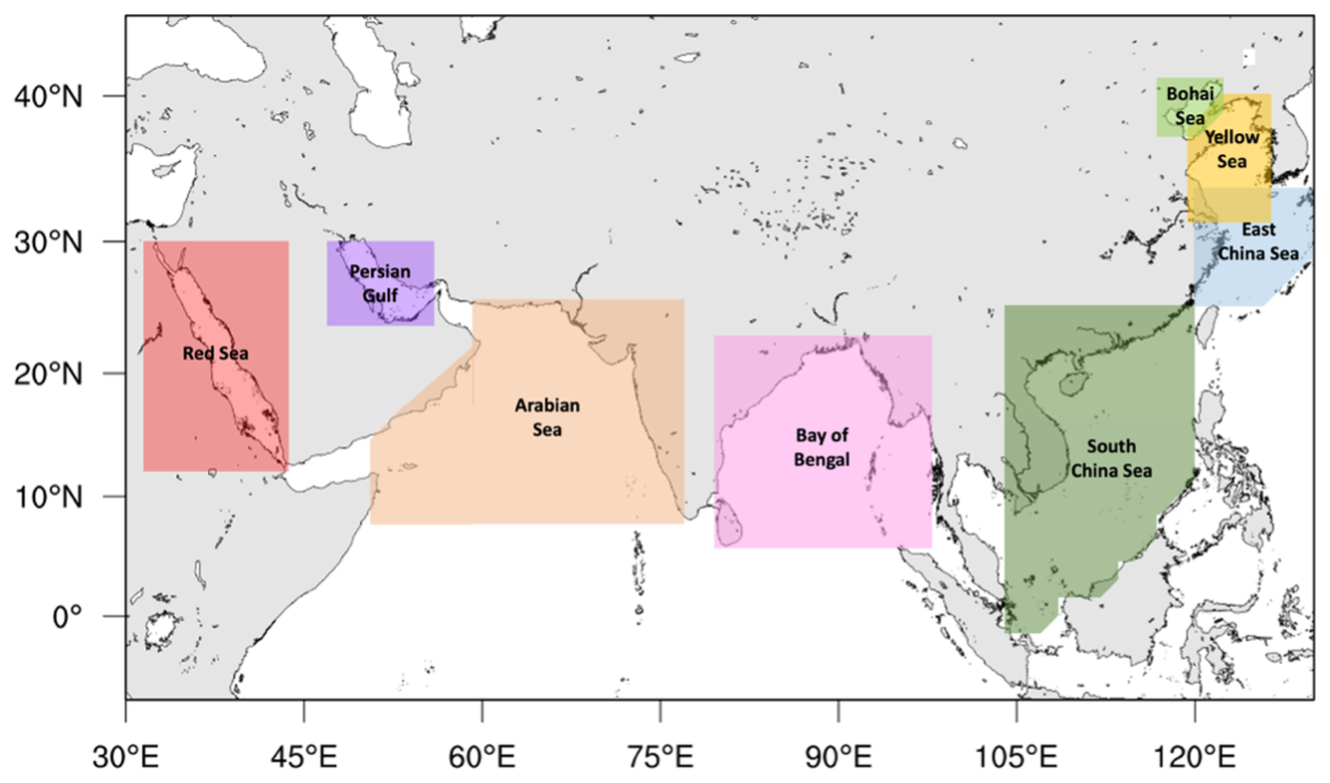
Figure 1 Areas of interest within the CESR domain used for the sub-regional analysis with satellite altimetry data: Red Sea, Persian Gulf, Arabian Sea, Bay of Bengal, South China Sea, East China Sea, Yellow Sea, and Bohai Sea.

Figure 2 presents the time series (1993–2023) of yearly mean sea level anomalies, averaged over the areas of interest. The global time series is corrected for GIA effects using the ICE5G-VM2 GIA model (Peltier, 2004). Linear sea-level trends are calculated for three consecutive 11 year intervals (1993–2003, 2003–2013, and 2013–2023), with each period including an overlapping year to ensure continuity in the analysis and reduce the influence of interannual variability. The associated standard errors are provided in Table 1.

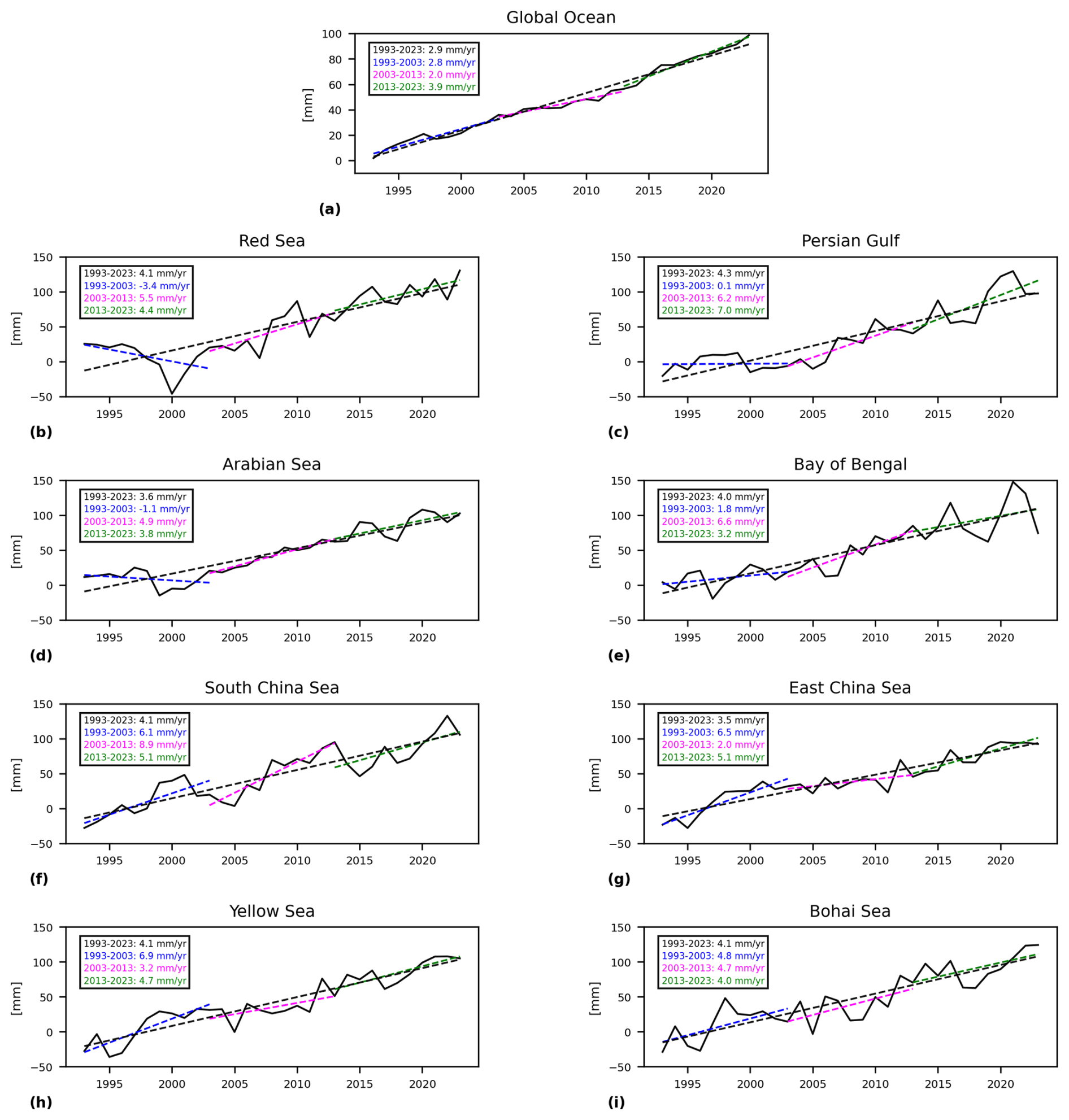
Figure 2 Time series (1993–2023) of yearly mean sea level anomalies (black curve) derived from satellite altimetry SLA and averaged over (a) Global Ocean, (b) Red Sea, (c) Persian Gulf, (d) Arabian Sea, (e) Bay of Bengal, (f) South China Sea, (g) East China Sea, (h) Yellow Sea, and (i) Bohai Sea. Coloured dashed lines indicate linear trends computed over three successive periods (1993–2003, 2003–2013, and 2013–2023). The overall linear trend over the full analysis period is also shown as a dashed black line. SLAs are based on the CMEMS product SEALEVEL_GLO_PHY_CLIMATE_L4_MY_008_057.

Table 1 SLA trends obtained from satellite altimetry (mm yr⁻¹) covering the areas of interest (Fig. 1) during 1993–2023, 1993–2003, 2003–2013 and 2013–2023. Bold values indicate statistically significant trends (p < 0.05).

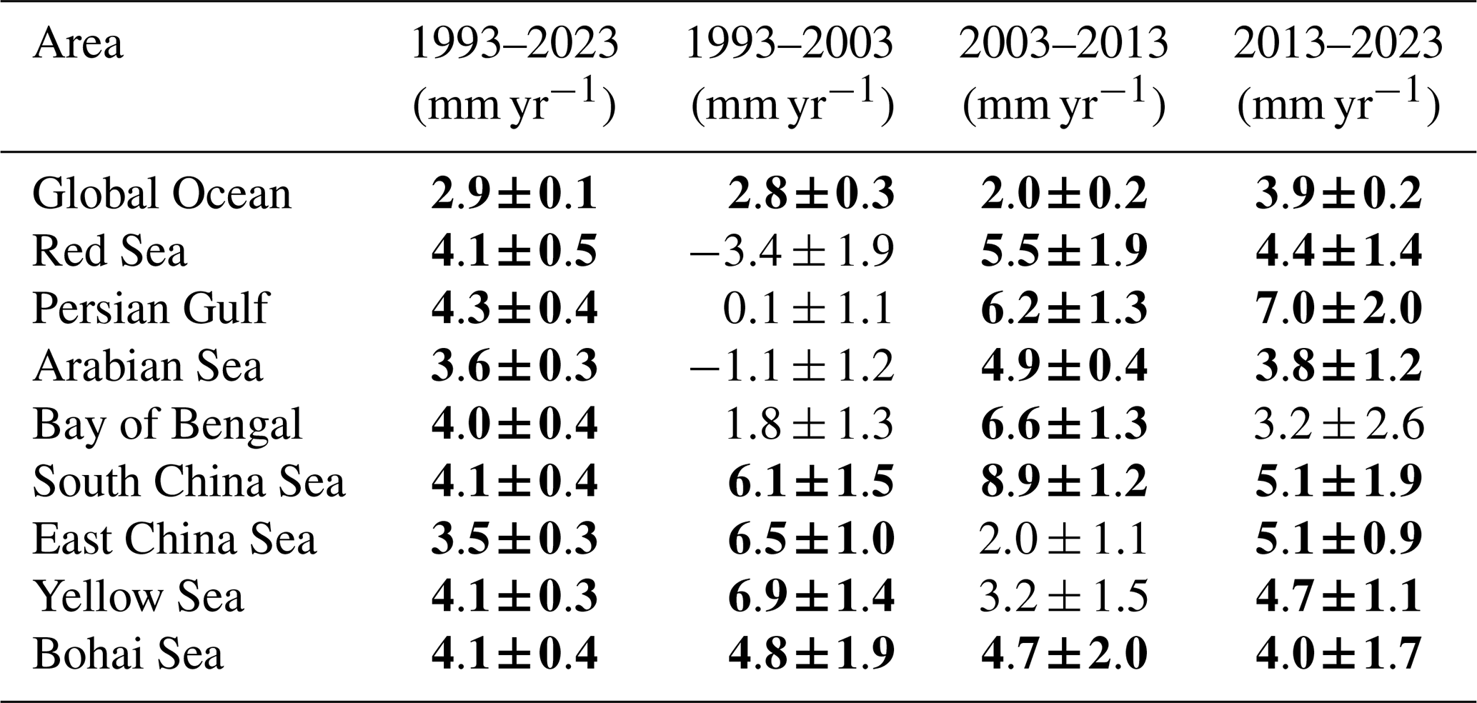
During the full period (1993–2023), SLA trends across the CESR sub-regions are 20 %–45 % higher than the global mean trend, with significant spatial and distinct decadal patterns. In the first decade (1993–2003), the four Indian Ocean sub-regions exhibit lower trends compared to the global mean, while the four Pacific sub-regions display higher trends.

Mean SLA trends increase eastward, from a minimum of −3.4 mm yr⁻¹ in the Red Sea to a maximum of 6.9 mm yr⁻¹ in the Yellow Sea, before slightly decreasing in the Bohai Sea (4.8 mm yr⁻¹). By the second decade (2003–2013), the spatial distribution shifts: regions like the Persian Gulf and Bay of Bengal, previously exhibiting low trends, become areas of maximum SLA trends, while the East China and Yellow Seas experience declining trends. The SLA trend increases markedly in the Red Sea, Persian Gulf, Arabian Sea, Bay of Bengal, and South China Sea, whereas the East China and Yellow Seas exhibit a slowdown. In the most recent decade (2013–2023), SLA trends decreased in five sub-regions (Red Sea, Arabian Sea, Bay of Bengal, South China Sea, and Bohai Sea) while increasing in the Persian Gulf, East China Sea, and Yellow Sea (Fig. 3).

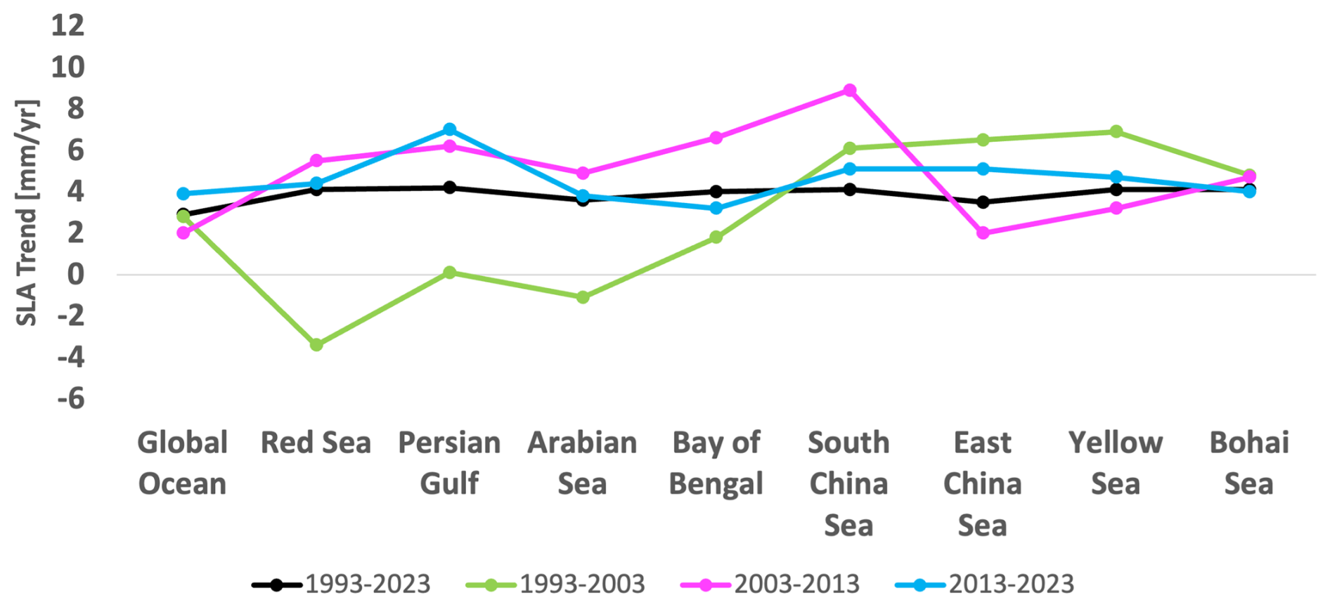
Figure 3 Regional mean sea level trends obtained from satellite altimetry for the Global Ocean and the CESR sub-regions shown in Fig. 1, computed over the periods 1993–2023, 1993–2003, 2003–2013 and 2013–2023. Data source: Copernicus Marine Service (CMEMS).

While these trends are indicative of significant decadal variability, not all trends meet the statistical significance threshold (p value < 0.05). Statistically significant trends confirm consistent and systematic changes in sea level trends by decade and across regions. Notably, the East China Sea, Yellow Sea and Bohai Sea show a decadal trend slowdown in the second (2003–2013) and third decade (2013–2023) with respect to the first one (1993–2003). Consistently with the decadal variability discussed above, the weak or near-zero sea level trends observed in the Red Sea, Persian Gulf, Arabian Sea and Bay of Bengal during the first decade (1993–2003) are primarily attributable to regional atmospheric forcing, steric effects and ocean mass redistribution, rather than to limitations of the multi-mission altimetric observing system, whose long-term stability and cross-mission consistency have been extensively validated (Cazenave et al., 2018).

The observed decadal variability in SLA trends across the CESR domain arises from complex interactions between natural and anthropogenic factors. Steric changes (thermal expansion and salinity variations) and ocean mass redistribution, due to ice melt and terrestrial water storage, are primary drivers of global SLA trends (Cazenave and Moreira, 2022). Regional atmospheric and oceanic processes, such as evaporation, precipitation and runoff variability, further influence regional SLA trends. For instance, the mass transport across the lateral boundaries of the regions, due to decadal changes in wind-driven circulation, significantly affects SLA trends in specific areas (Cazenave et al., 2014, Borile et al., 2025).

Large-scale climate oscillations, including the El Niño–Southern Oscillation (ENSO), Indian Ocean Dipole (IOD), and North Atlantic Oscillation (NAO), further modulate regional ocean dynamics, contributing to SLA variability (Cazenave and Moreira, 2022). Additionally, monsoon-driven processes exert a strong influence on sea level variability in several CESR sub-regions, particularly in the Arabian Sea, Bay of Bengal, South China Sea, East China Sea, and Yellow Sea, where seasonal wind forcing and associated circulation changes play a key role (Han et al., 2010; Huang et al., 2024).

Figure 4 illustrates the spatial distribution of SLA trends (mm yr⁻¹), computed at each grid point of the altimetry product, for 1993–2023, overlaid with climatological surface currents from the Global Multi-Year product (GLOBAL_MULTIYEAR_PHY_001_030) by CMEMS. Minimum SLA trends (2–3 mm yr⁻¹) are observed near western boundary currents like the Kuroshio and its branches. In contrast, SLA trends exceed 4 mm yr⁻¹ along the coasts of the Yellow and East China Seas. Although the spatial patterns shown in Fig. 4 are derived from the gridded altimetry product, coastal values should be interpreted with caution because satellite altimetry may be affected by land contamination near the shoreline. The South China Sea displays maximum SLA trends in its open-ocean regions, which may be associated with large-scale circulation variability and exchanges with the western Pacific through the Luzon Strait, as suggested by previous studies (Qiu and Chen, 2010; Sprintall et al., 2014). Beibu Bay and Vietnam's eastern coastal waters exhibit trends around 4 mm yr⁻¹, while the Gulf of Thailand shows lower trends (∼3 mm yr⁻¹). The largest SLA trend (∼5 mm yr⁻¹) is found in the northern and northwestern Bay of Bengal, rather than being uniformly distributed across the basin. These results are based on regional spatial averages and are therefore not significantly affected by land contamination issues in satellite altimetry near the coast

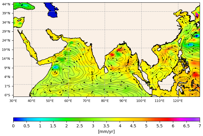
Figure 4 Absolute Sea level trend [mm yr⁻¹] computed from monthly mean satellite altimetry data (seasonal cycle removed) over the period 1993–2023 using the CMEMS product SEALEVEL_GLO_PHY_CLIMATE_L4_MY_008_057. Climatological surface currents from the CMEMS Global Multi-Year product (GLOBAL_MULTIYEAR_PHY_001_030) are overlaid as streamlines. The circulation features shown represent annual-mean conditions.

3.1.2 Relative sea level

Tide gauges, which have been operational since the 18th century, provide localized, long-term insights into sea level dynamics, supporting research on climate change, ocean circulation, extreme events, and coastal hazard assessments. Despite their invaluable role, tide gauge measurements must be integrated with satellite altimetry data to offer a comprehensive view of sea level changes, particularly in regions with complex oceanographic and atmospheric dynamics, such as the CESR.

For this study, a subset of tide gauge stations from the RLR dataset with records starting in 1993 was selected (Fig. 5). Observations from these stations were compared with data from the nearest altimetry grid points.

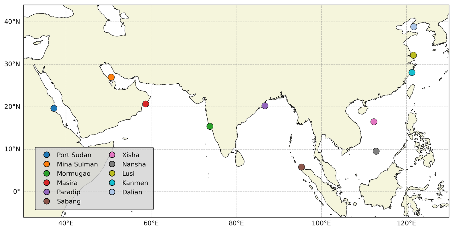
Figure 5 Geographical distribution of the selected PSMSL tide gauge stations used in this study.

Figure 6 shows the time series for both datasets, highlighting their overall consistency. However, some discrepancies were identified in some stations due to local vertical land movements. The comparison of SLA nearest grid points time series with tide gauges data reveal strong correlations (0.9–1.0) for most stations, except for Sabang (Bay of Bengal, corr. coef. 0.6) and Masira (Arabian Sea, corr. coef. 0.1).

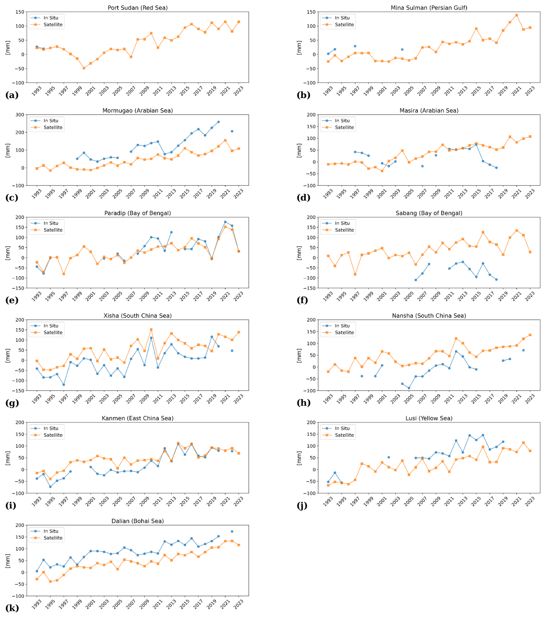
Figure 6 Time series (1993–2023) of annual mean sea level anomalies (mm) at the platforms: (a) Port Sudan (Red Sea), (b) Mina Sulman (Persian Gulf), (c) Mormugao (Arabian Sea), (d) Masira (Arabian Sea), (e) Paradip (Bay of Bengal), (f) Sabang (Bay of Bengal), (g) Xisha (South China Sea), (h) Nansha (South China Sea), (i) Kanmen (East China Sea), (j) Lusi (Yellow Sea), and (k) Dalian (Bohai Sea). Tide gauge stations observations (blue) represent relative sea level, while satellite altimetry (orange) absolute sea level. Data sources: PSMSL and Copernicus Marine Service (CMEMS).

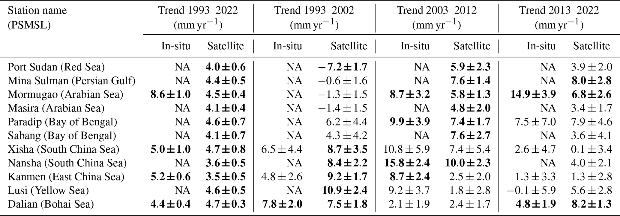
Table 2 provides a detailed comparison of sea level trends and associated uncertainties (expressed as standard errors) for each selected PSMSL station using both in-situ and satellite data over multiple periods: 1993–2022, 1993–2002, 2003–2012, and 2013–2022. Altimetric trends were computed at the grid points nearest to the tide gauge stations, while in-situ trends were excluded where yearly observations were less than 70 % of the expected data for the reference period. Notably, 2023 data were omitted from the analysis, as only the Paradip station (Bay of Bengal) reported observations for that year. Bold p values in Table 2 indicate statistically significant trends, emphasizing the reliability of those results.

Table 2 Sea level trends with standard errors calculated for each selected PSMSL station using in-situ and satellite data over the periods 1993–2022, 1993–2002, 2003–2012, and 2013–2022. Altimetric trends were computed at the grid points nearest to the tide gauge, while in-situ trends were excluded (NA) where yearly observations were < 70 % of the expected data for the reference period. Bold indicate statistically significant trends. In-situ trends represent relative sea level change and may include local vertical land motion.

3.2 Extreme sea level events

During a severe storm, water levels at the coast will rise as a result of atmospheric pressure changes and the winds (Pugh and Woodworth, 2015). This causes storm surges, resulting in water levels that can be up to several meters above Mean Sea Level (MSL), especially when coinciding with high tide. In addition, there might also be coastally trapped non-isostatic signals from large scale pressure patterns that could amplify the local wind and tidal effects (Zhao et al., 2017; Park et al., 2022).

The CESR region is indeed prone to extreme sea levels, and several factors contribute to this vulnerability, among others tropical and extratropical cyclones. It is reported that in the Red Sea, the extreme sea level in the basin is about 0.30–0.50 m, and the extreme sea level in the Gulf of Suez is about 0.85 m (Antony et al., 2022). In the Persian Gulf, the probability of storm surges is low. However, Lin and Emanuel (2016) have shown that tropical cyclones could occur in that region, potentially causing surges of up to 4 m in Dubai, but with a return period of more than 10 000 years. The Bay of Bengal is an area particularly prone to high extreme sea levels (Dube et al., 2009; Lewis et al., 2013), experiencing, on average, five surge events per decade exceeding a surge level of 5 m (Needham et al., 2015). Regions in the North-western Pacific, including China and the Philippines, can experience tropical cyclones and high storm surges (Zhang et al., 2015; Fang et al., 2021). For example, the once-in-50 years extreme sea levels along the coastline of China from the south of Shandong Peninsula to the Beibu Gulf, range between 1.6 and 3.2 m (Zhang and Sheng, 2015).

The analysis of the extreme sea levels is done using the GTSMip and COAST-RP data sets as well as tide gauge stations. It shows that the 100 year high water level events reach 3 m in the mouth of the Bay of Bengal, along the western coast of the Yellow, East and South China Seas, while lower water levels can also be observed in other regions such as the Red Sea. In addition, tides can significantly contribute to extreme sea level events. When comparing the Mean Highest High Water (MHHW) and Highest Astronomical Tide (HAT) in Fig. 7 with the 1 in 100 year water levels (Fig. A4), areas such as the Gulf of Khambhat (India), Andaman Sea bordering Myanmar, west of North and South Korea, and areas along the coast of the East China Sea between Shandong and Fujian province experience tides exceeding 2 m. These regions also similarly experience high surge levels, as shown in Fig. A4 where levels can nearly reach or exceed 3 m.

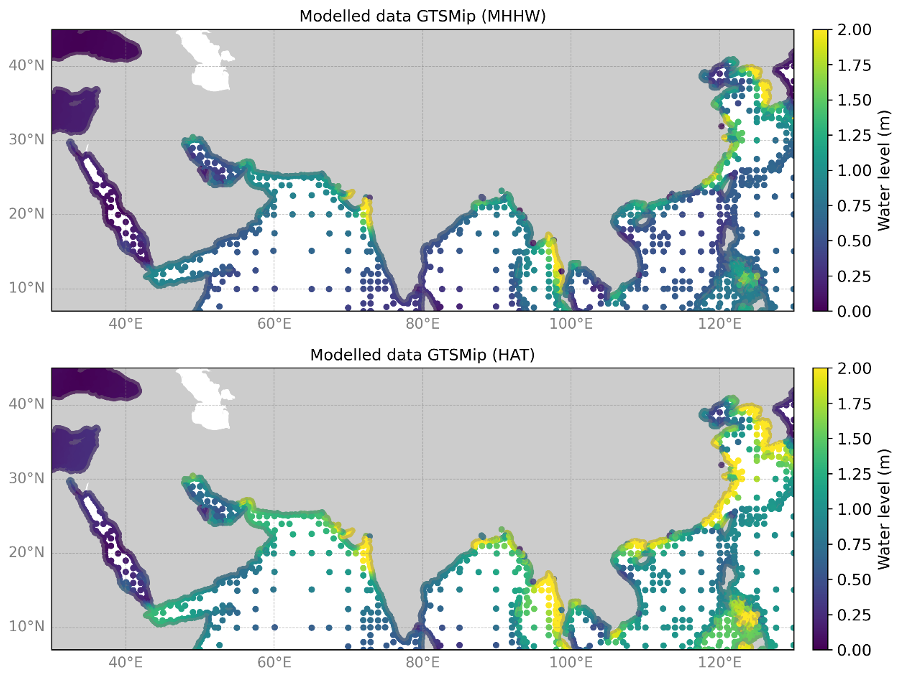
Figure 7 Overview of the tidal levels in the region over the period 1985–2014 derived from the GTSMip dataset. (Top) Mean Higher High Water (MHHW). (Bottom) Highest Astronomical Tide (HAT).

Validation of GTSMip and COAST-RP datasets are presented in Appendix A, including comparison between tide gauge data and error metrics for both these datasets (Fig. A3), as well as an inter-comparison between GTSMip and COAST-RP data (Fig. A4). This indicates that while the overall performance is good, considerable differences and uncertainties may arise as a result of both methodological differences and limitations in underlying data.

Figure 8 shows that the return period levels of extreme sea levels at several selected tide gauge stations are generally consistent, especially for lower return periods, but there are also relevant differences. For Zhapo, Hong Kong and Shanwei the observations show overlap with the modelled data. For higher return periods, the deviations are somewhat higher, but this is likely caused by differences in the length of timeseries. For Zhapo there are tropical cyclones that can cause much higher water levels than measured in the observational record. Also, for Hong Kong and Shanwei, the values of COAST-RP are higher than GTSMip, with larger deviations for higher return periods. The large deviations for large return periods highlight the problem of small sample size when solely relying on historical tropical cyclones. The results indicate the need for the use of synthetic tropical cyclones to obtain robust estimates of extreme sea levels. The result also highlights the uncertainty that comes from different extreme value analysis methods, as was also shown in the global analysis by Wahl et al. (2017). For Xiamen, the results show that while the slope of the extreme value distribution of the modelled data agrees with the observations, there is an offset of about 0.3 m between the observations and the modelled data. Efforts are underway to try to harmonize the datum by removing the annual means, since this is potentially the reason for the discrepancy in the vertical datum. Other causes may include a strong seasonal component in mean sea level, driven by a process that is not resolved by GTSM. GTSM is a depth-averaged barotropic model and does not simulate density-driven processes nor include river inflows.

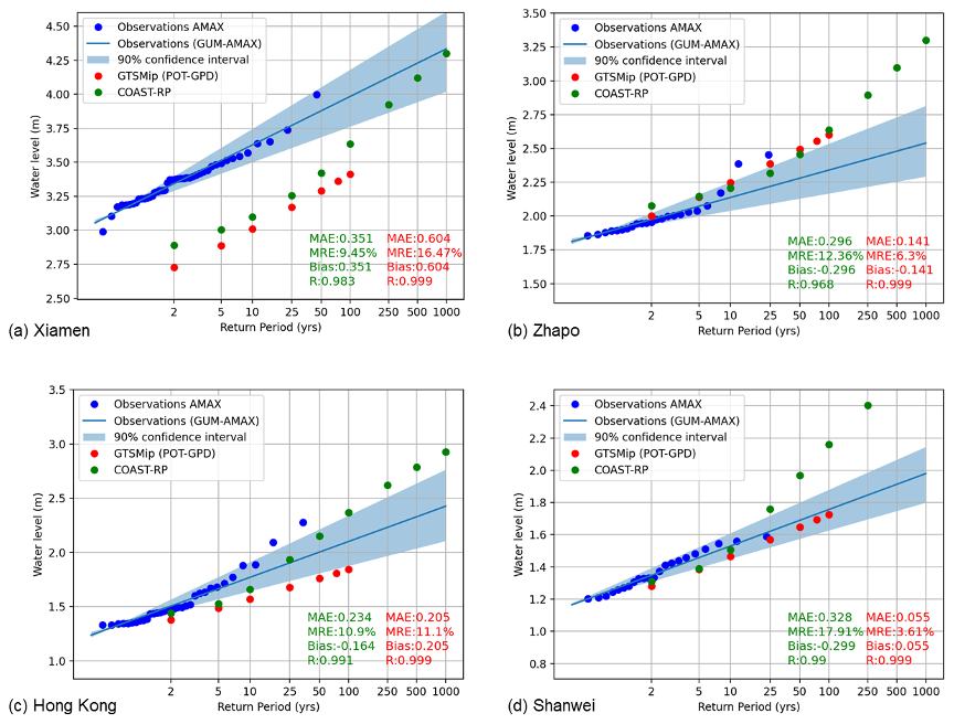
Figure 8 Extreme value plot for selected stations showing observations in blue (annual maxima in dots, line shows Gumbel fit, and 90 % confidence interval based on bootstrapping in shaded area), GTSMip in red, and COAST-RP in green.

4 Discussion

This study analyses sea level trends and extreme events along the China–Europe Sea Route (CESR) at decadal and multidecadal scales by integrating satellite altimetry, tide gauge observations, and hydrodynamic model reanalyses. The findings highlight the complexity of regional sea level change, which reflects the interplay of natural variability, anthropogenic forcing, and localized processes, with direct implications for coastal risk assessment and adaptation strategies.

Beyond the regional findings, this work contributes to the existing literature by providing a harmonized assessment of both mean sea level trends and extreme sea levels across multiple interconnected basins of the CESR. Unlike studies focused on single regions or individual components of sea level change, the present analysis combines multi-mission altimetry, long-term tide gauge data, and state-of-the-art global hydrodynamic models within a unified framework. This integrated perspective enables a consistent evaluation of decadal variability in both mean conditions and extremes across basins characterized by distinct dynamical regimes, revealing contrasts and commonalities that would not emerge from basin-specific analyses alone.

Over the 1993–2023 period, mean sea level trends in the CESR sub-regions exceed the global mean by approximately 20 %–45 %, with a clear eastward intensification. Pronounced decadal variability is evident, particularly in the East China Sea, Yellow Sea and Bohai Bay, where periods of trend slowdown may reflect changes in circulation affecting mass transport across open-ocean boundaries, regional water-cycle variability, and steric contributions.

In the North Indian Ocean sector, the results indicate signals consistent with positive acceleration; however, strong interdecadal variability prevents a robust quantification of acceleration at the regional scale. Rather than representing a uniform long-term acceleration, the observed patterns likely reflect the influence of large-scale regional processes. On the Pacific side of the CESR, including the South and East China Seas, periods of slowdown are observed and may be linked to interannual climate variability influencing circulation, water-cycle processes, and steric effects, consistent with findings for the global ocean (Cazenave et al., 2014) and for the Mediterranean Sea (Borile et al., 2025).

The mechanisms underlying this decadal variability warrant further investigation. Huang et al. (2024) reported a multidecadal sea-level decline in the Tropical Southwest Indian Ocean from the 1960s to the early 2000s, followed by a marked rise of 4.05±0.56 cm per decade, associated with shifts in atmospheric circulation and contributions from Ekman pumping and deep-water warming. Similar processes may contribute to the variability observed in the North Indian Ocean portion of the CESR. On the Pacific side, the decrease in mean sea level trends during 2003–2013 likely reflects combined effects associated with water-cycle redistribution, consistent with previously documented global patterns (Cazenave et al., 2014).

The comparison between satellite altimetry and tide gauge records underscores the importance of integrating absolute and relative sea level observations. While general agreement is observed at most locations, discrepancies arise in specific areas and are likely associated with local vertical land motion, seismic activity, and residual limitations of coastal altimetry in shallow and nearshore environments.

Extreme sea level analysis further reveals substantial regional contrasts in return periods and magnitudes. The Bay of Bengal and the northwestern Pacific emerge as hotspots of extreme sea levels, primarily driven by tropical cyclones and storm surges. Although the GTSM-based modelling framework reproduces the large-scale spatial patterns of extremes, differences persist due to known limitations, including the underestimation of storm winds in ERA5 and the absence of density-driven processes in the barotropic model configuration. The incorporation of synthetic cyclone tracks in the COAST-RP dataset substantially improves the representation of high-return-period events.

Overall, the combined use of satellite altimetry, tide gauges, and hydrodynamic models enables a comprehensive assessment of both gradual sea level rise and extreme coastal hazards along the CESR. This integrated framework provides a consistent basis for interpreting regional variability and supports the integration of return-period estimates with flood and impact models to evaluate population exposure and coastal risk under present and future sea-level rise scenarios.

5 Conclusions

This study underscores the importance of regional-scale analysis to capture the drivers of sea level change along the CESR region. The results highlight significant spatial and temporal variability in SLA trends across CESR sub-regions, driven by the interplay of processes related to the regional water balance, ocean circulation, and steric effects.

Higher-resolution and region-specific datasets and models are essential for further disentangling natural variability from anthropogenic forcing and for improving the representation of coastal and extreme sea level processes. Such advancements are vital for enhancing coastal resilience, informing navigation strategies, and supporting adaptation planning along this economically and geopolitically significant maritime corridor.

Appendix A: Model validation

To validate the return periods extracted from GTSM, hourly observations from tide gauge stations are used. In this case, observations are retrieved from the University of Hawaii Sea Level Center Dataset (UHSLC, https://uhslc.soest.hawaii.edu/datainfo/, last access: 9 April 2026). There are 52 tide gauge stations in the area of interest (between 7–45° N and 30–130° E). The total number of records selected for this analysis is 15, using only the tide gauge stations with a minimum record of 25 years and a maximum of 20 % of missing data. For each station, the annual mean is removed to reference all data to the same vertical datum. Extreme value analysis is used to estimate the water levels corresponding to different return periods (see Sect. 2.3).

A comparison between the return periods computed for the tide gauge stations and the GTSM model demonstrated good performance overall (Fig. A3). The correlation coefficients of the return periods from the tide gauge stations (using POT and fitting Gumbel distribution to the annual maxima) and GTSM model values against their respective water levels yielded a correlation coefficient of 0.96 and >0.99. The mean bias (MB) is 0.10 m for COAST-RP and 0.14 m for GTSMip. The mean absolute error (MAE) is 0.37 (SD 0.33) for COAST-RP and 0.33 (SD 0.34) for GTSMip. It shows that, on average, for the 1 in 100 year return level the datasets are comparable in performance. The middle and bottom panels in Fig. 8 show a comparison of the observed return levels with modelled return levels from, respectively, GTSMip and COAST-RP. It shows that the water level is underestimated at most locations, but that for many stations, the errors are smaller than 0.5 m. Errors could be larger in regions prone to tropical cyclones, such as the Philippines. In these regions, a single event in the observations can heavily influence the return period estimations. On the one hand, those extremes will likely be underestimated in the GTSMip dataset which is based on the ERA5 climate reanalysis forcing.

Figure A1 Grid of the Global Tide and Surge Model for Southeast Asia. See more https://publicwiki.deltares.nl/display/GTSM/Model+description+and+development (last access: 9 April 2026).

The difference between GTSMip (upper panel) and COAST-RP (middle panel) in Fig. A4 reflects the larger sample for tropical cyclones and differences in the extreme value analysis. With a value exceeding 0.5 m, the differences between the two datasets are relatively large. GTSMip mostly shows an underestimate compared to COAST-RP, with the largest difference in the Philippines, Cambodia and near South Korea, but there are also regions of over-estimates such as the Pacific Kuril Islands. The probabilities in COAST-RP are more robust than for GTSMip and the COAST-RP is expected to perform better in regions prone to tropical cyclones. Basically, the 40 years of ERA5 simulations are too short to estimate tropical cyclone probabilities. In other regions, the differences are much smaller (e.g., Red Sea region) and are mainly caused by a difference in the methodology used for the extreme value analysis.

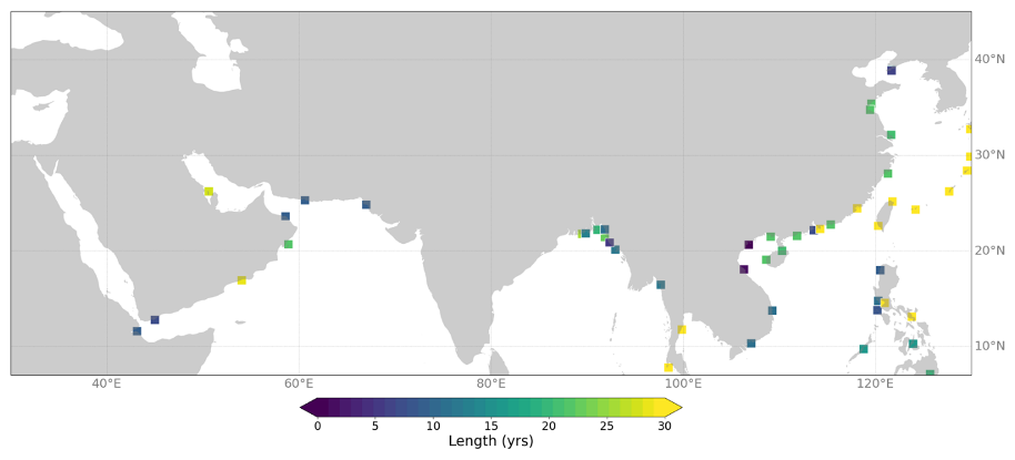
Figure A2 Map of available tide gauge stations of the UHSLC dataset and their corresponding record length (years). From the available tide gauge stations, only stations with more than 25 years of data were used for the validation in this study.

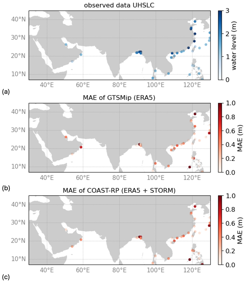
Figure A3 Full dataset of observed and modelled water levels corresponding to a return period of 100 years. The top panel shows the observed water levels from UHSLC. The middle and the lower panels show the Mean Absolute Error (MAE) for GTSMip and COAST-RP respectively.

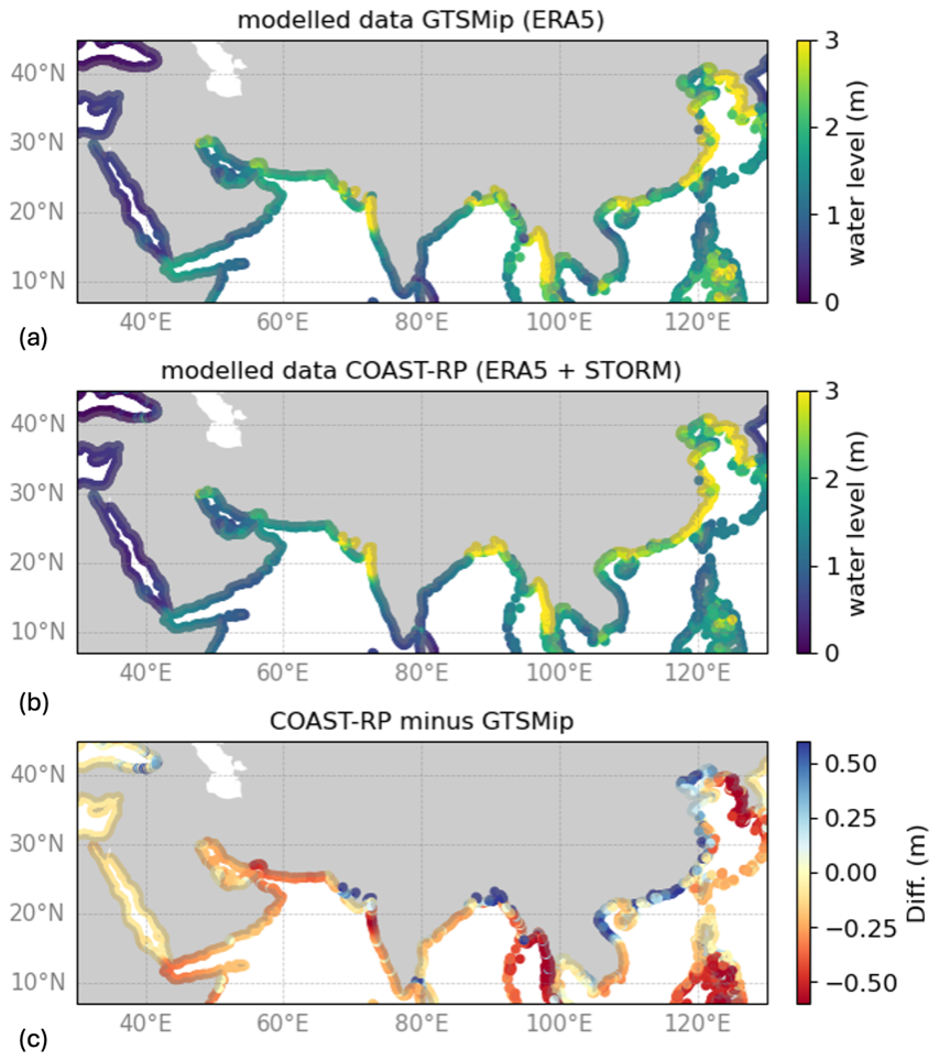
Figure A4 Overview of 1 in 100 year exceedance events for extreme surges. (Top) Extreme surge levels from GTSMip forced with ERA5. (Middle) Extreme surge levels from Coast-RP. (Bottom) Difference between GTSMip and Coast-RP surge levels. Return levels are below 1 m for most of the coastline of the Red Sea (e.g., Egypt, Sudan, Yemen, eastern Saudi Arabia). Values between 1 and 2 m are seen for most of the Persian Gulf (e.g., Iran, Oman, and eastern Saudi Arabia), Arabian Sea (e.g., Pakistan), southwest coast of the Bengal Bay (India) and parts of the South China Sea (e.g., Vietnam). Regions where the 1 in 100 year water levels exceed 2 m includes northern part of Bay of Bengal (Bangladesh), north-eastern part of the Arabian Sea (west India and southeast Pakistan), Gulf of Thailand (Cambodia) and the Yellow Sea (northern China).