Towards global sensitivity analysis of large-scale flood loss models

Flood loss models are increasingly used in the (re)insurance sector to inform a range of financial decisions, and more broadly in research and policy analysis to understand present-day and future flood risk trends. These models simulate the interactions between flood hazard, vulnerability and exposure over large spatial domains, requiring a range of input information and modelling assumptions. Due to this high level of complexity, evaluating the impact of uncertain input data and assumptions on modelling results, and therefore the overall model “acceptability”, remains a very complex process. In this paper, we advocate for the use of global sensitivity analysis (GSA), a generic technique to analyse the propagation of multiple uncertainties through mathematical models, to improve the sensitivity testing of flood loss models and the identification of their key sources of uncertainty. We discuss key challenges in the application of GSA to large-scale flood loss models, propose pragmatic strategies to overcome these challenges, and showcase the type of insights that can be obtained by GSA through two proof-of-principle applications to a commercial model, JBA Risk Management's flood loss model, for the transboundary Rhine River basin in Europe, and Queensland in Australia.

1 Introduction

Floods are among the most widespread risks to human lives, infrastructure and property worldwide. Between 2000 and 2019, floods affected 1.65 billion people, accounting for 41 % of all people affected by natural disasters (CRED-UNDRR, 2020) or what are increasingly described as “human-made disasters” (see Otto and Raju, 2023). Floods were responsible for 9 % of all disaster-related deaths and caused 22 % (USD 651 billion) of all disaster related damages (CRED-UNDRR, 2020). Their impact continues to grow globally (Kreibich et al., 2022) and flood risk is set to increase even further under the combined effect of more extreme weather and urban development into flood-prone areas (Merz et al., 2021). Increasing the penetration of flood insurance and reducing the level of uninsured flood risk – the “protection gap”, or proportion of risk that remains uninsured – will be crucial for adaptation to such growing levels of risk (Tesselaar et al., 2022; Aerts et al., 2024).

To close the protection gap, insurers need to quantify the risks associated with underwritten policies. To do so, they increasingly rely on probabilistic models of natural hazard impacts, which enable them to estimate expected losses in a much more robust way than by extrapolating from limited and- often inaccurate historical loss data. These models, known in the industry as “loss models” or “catastrophe models”, are used to inform a range of decisions, from pricing an individual policy to optimizing reinsurance at company level (Mitchell-Wallace et al., 2017). They calculate the total value of expected losses that an insurer may face from a given region over a specified time horizon. This is achieved by combining three core components: (i) the hazard module, which estimates the spatial distribution of flood intensities (a measure chosen to represent the strength of the potential for harm, for example flood depths); (ii) the exposure module, which locates insured assets and their values; and (iii) the vulnerability module, which quantifies the damages to the exposed assets caused by the floods (Grossi and Kunreuther, 2005). Beyond the insurance sector, flood loss models are increasingly important also in research and policy analysis to increase our understanding of present and future risk trends (e.g. see discussion by Ward et al., 2015) and to support policy development (e.g. see the PESETA programme by the European Commission Joint Research Centre, EC JRC, 2026).

While loss models are continuously revised and upgraded, their evaluation remains an open challenge. Currently there are no prescribed or standardized validation tests¹ for acceptance of a particular flood loss model in the insurance industry (Franco et al., 2020) despite the many limitations in both understanding and data around flood processes and impacts (Lighthill Risk Network, 2019). Such lack of common evaluation approaches is not unique to the insurance sector as “validation is perhaps the least practised activity in current flood risk research and flood risk assessment” (Molinari et al., 2019).

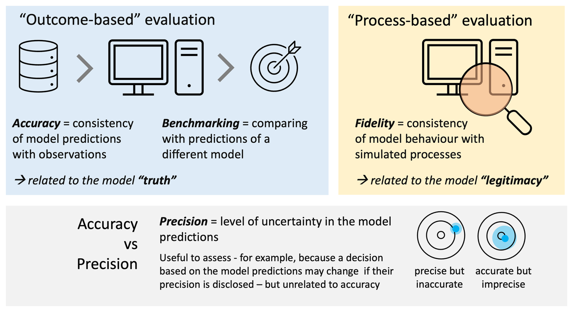
Figure 1 Conceptual approaches to model evaluation: outcome-based (left) and process-based (right). Sensitivity analysis contributes to the latter, by providing a mechanism to assess model fidelity. While shown here in the context of flood loss models, the framework applies more broadly.

In principle, there are different approaches to model evaluation, which broadly fall into two categories (Merz et al., 2024): “outcome-based” evaluation, where the emphasis is on the modelling outputs, i.e. the loss predictions, and on checking whether they are consistent with either historical observations (hence establishing the model accuracy) or other models' predictions (benchmarking); and “process-based” evaluation, which focuses on checking the quality of the modelling process itself, rather than its outcome (Fig. 1). An example of the latter is sensitivity analysis (or “sensitivity testing”), which involves changing the model's input data, internal parameters and/or assumptions, and checking that the output response to such changes align with the user expectations (in terms of direction of change, relative magnitude etc.). The aim is to establish the model's fidelity, i.e. the consistency of the model behaviour with the user's understanding of the simulated processes (Wagener et al., 2022) and use that as a basis for its legitimacy. Another aim of sensitivity analysis is to identify the inputs/assumptions that mostly control the output uncertainty and hence prioritise efforts towards improving the model precision (Fig. 1). For example, if a particular input is shown to have little influence on the output uncertainty, investing in acquiring better quality data for that input may be unjustified.

Figure 2 Approaches to Sensitivity Analysis: local vs. global.

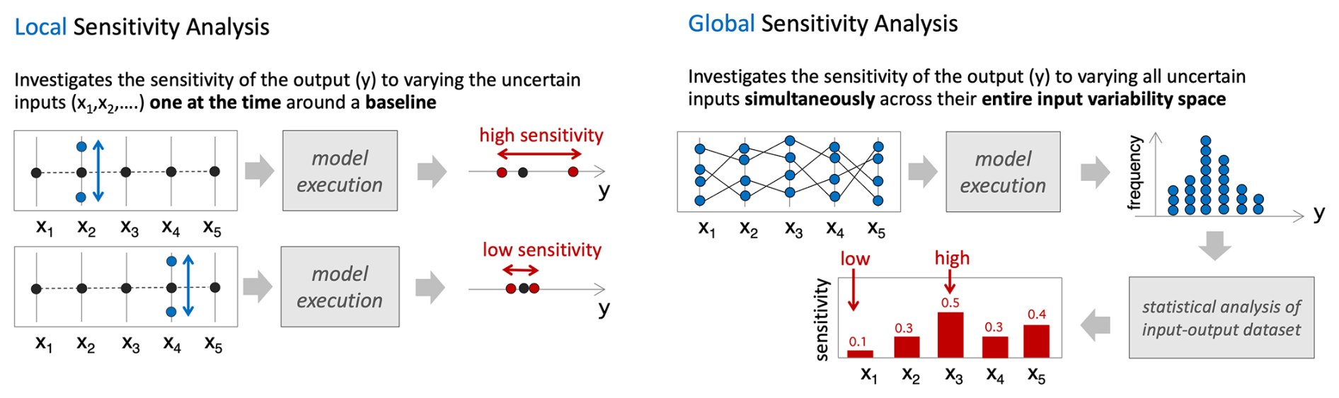
In practice, testing flood loss model accuracy can be very difficult because historical loss data are scarce and, even when available, the associated hazard intensity and exposure may not be fully known. Therefore, the model's inability to reproduce observed losses may be equally attributed to a model deficiency or to gaps and errors in the input data². As for sensitivity analysis, it is routinely used but often limited to investigating the effects of varying input data, typically the exposure portfolio. This is due to the “black-box” nature of most commercial loss models, which do not allow the user to change the parameters and assumptions embedded in the hazard and vulnerability components. Indeed, a recent paper on the state-of-art of insurance loss modelling concluded that “the assessment of uncertainty all along the modelling chain constitutes the loss modelling framework's notable shortcoming and the one that requires further investigation” (Déroche, 2023). The need for more transparency in modelling has also been identified as a key priority for improvement of climate risk assessment in relation to the rapidly emerging regulation for climate-related financial disclosure (Arribas et al., 2022). From a methodological perspective, another problem with the sensitivity testing prevailing in the industry is that it follows a “local” approach (Fig. 2) whereby output sensitivity is assessed by varying inputs “one-at-the-time” from a default value (“baseline”). There are two major limitations to this approach. First, it does not capture interactions between model inputs that may amplify or dampen the effects of individual input variations – a common feature of complex, non-linear models. Second, its results are conditional on the chosen baseline, leaving the question open of how different the sensitivity assessment would be if using a different baseline (Fig. 2).

In this paper, we argue that flood loss models should be made more transparent to their users and that their sensitivity testing should be made more robust. In particular, we suggest that local, one-at-the-time sensitivity analysis should be replaced by a global sensitivity analysis (GSA) approach. GSA is a methodology to systematically investigate how simultaneous variations in the inputs of a model (including parameters, forcing inputs, or initial conditions) affect the model outputs. A typical result of GSA is a set of sensitivity indices each measuring the relative contribution of every varied input to the uncertainty in each model output (Saltelli et al., 2007). Note that, different to local approaches, in GSA all inputs are varied simultaneously within their variability space without any baseline being required (Fig. 2).

While GSA is increasingly used for investigating uncertainty propagation in hydrological modelling (e.g. Song et al., 2015) and, to a lesser extent, flood inundation modelling (e.g. Savage et al., 2016), applications to flood loss models have been few and limited to relatively small spatial domains (e.g. de Moel et al., 2014, for a 40 km×60 km region in the Netherlands, Hosseini-Shakib et al., 2024, for a 3 km×5 km borough in Pennsylvania, Tate et al., 2014, for the Iowa city area in the US) or simplified strategies to understand flooding potential at global scale (Devitt et al., 2023). An interesting application is presented by Metin et al. (2018), who used GSA to identify the drivers of future flood risk in the Mulde catchment, a 7000 km² sub-basin of the Rhine. Their work shows yet another use of GSA, whereby the analysis is applied with the aim of learning about risk drivers in the real system – under the (implicit) assumption that the model is a valid representation of that system – instead of learning about the model and thus informing its validation and future improvements – as done in the other referenced studies, and in this one.

The limited uptake of GSA in the flood loss modelling sector may be due to a lack of awareness of the advantages of global over local sensitivity analysis – a common issue across many modelling sectors (Saltelli et al., 2019) – but also to the specific difficulties encountered in applying GSA to large-scale models. These include three key challenges: the potentially very large number of input uncertainties that one could analyse; the “uncertainty about the uncertainties”, i.e. the fact that, for many of those input uncertainties, the analyst may not be able to state what variations would be reasonable and what would not; and the computational burden of running the model hundreds or even thousand times, when each model execution may take from several minutes to hours.

The goal of this paper is to discuss how we can begin to tackle these challenges and showcase the type of results that could be obtained through two proof-of-principle applications to a commercial model – JBA Risk Management's (hereafter JBA's) flood loss model – applied to two large domains: the transboundary Rhine River basin in Europe and Queensland in Australia. In the next two sections, we will describe the key working principles of large-scale flood loss models and of the GSA methodology for context. We will then discuss in more detail the key challenges in applying GSA to large-scale flood loss models and possible solutions. Last, we will show the results of two illustrative applications of GSA to JBA's flood loss model, a large-scale commercial flood loss model used by insurers and risk analysists for local- (e.g. D'Ayala et al., 2020; Galloway et al., 2025) and large-scale (e.g. Kay et al., 2018; Becher et al., 2023) risk assessments. The first application to the whole Rhine River basin in Europe will showcase how GSA can be used to understand the relative importance of hazard, vulnerability and exposure uncertainties in a consistent way across a large spatial domain, as a way to identify priorities for model improvement. The second application to Queensland state in Australia will showcase how GSA provides a framework to consistently compare present-day uncertainties in vulnerability and exposure with uncertainty about future climate.

2 High-level description of a large-scale Flood Loss Model

Flood loss models use multiple components to estimate flood risk in terms of monetary losses induced by floods (Fig. 3). In this paper, we will use JBA Risk Management's flood loss model, a proprietary model designed to quantify flood losses by integrating hazard, exposure, and vulnerability components. This section briefly describes the model, although the focus is not on the specific details of JBA model itself but rather the generic structure and key components of any flexible loss modelling framework used in (re)insurance, financial, development, and disaster risk reduction sectors. In essence, the loss L_s,k for a single exposed asset s and a single flood event k is given by

$$\begin{array}{}\text{(1)}& L_{s,k}={\text{EV}}_s\times \text{DR}\left({\text{FD}}_{s,k}\right),\end{array}$$

where EV_s is the asset's value, FD_s,k is the flood depth of the event k at the asset s, and DR(⋅) is the damage ratio, given by a vulnerability curve (or “depth-damage function”) that returns a fraction between 0 and 1 as a function of the flood depth. For a given spatial domain, Eq. (1) is applied for all the exposed assets and all flood events in a synthetic event catalogue spanning a long time horizon (10 000 years in our study). Such a catalogue enables estimation of the full distribution of annual losses, including both frequent and rare events. In this context, probabilities are often expressed in terms of a return period (RP), where, for instance, a 200 year event corresponds to a probability p=0.005 via the relationship $\text{RP}=\mathrm{1}/p$.

Insurance sector users are typically interested in two summary statistics of the annual loss distribution: the average annual loss (AAL) and the loss exceedance (LE(p)), which indicates the annual loss that is exceeded with probability p (e.g., the 200 year loss). Loss statistics are typically aggregated spatially, such as into CRESTA (Catastrophe Risk Evaluation and Standardizing Target Accumulations) zones (https://about.cresta.org/, last access: March 2026), which are standardised regions used in the insurance industry (Grossi and Kunreuther, 2005).

The AAL for a CRESTA zone C is calculated as

$$\begin{array}{}\text{(2)}& {\text{AAL}}_C={\sum }_{s\in C}{\sum }_k{p}_{s,k}{L}_{s,k},\end{array}$$

where p_s,k is the annual probability of event k affecting asset s.

To quantify tail risk, the loss exceedance curve (EP curve) is constructed by simulating total annual losses L_C,Y for each zone C and year Y in the catalogue, then empirically estimating their exceedance probabilities. Formally, the exceedance value LE_C(p) is defined by

$$\begin{array}{}\text{(3)}& {\text{LE}}_C\left(p\right)=X\text{such that}\mathbb{P}(L_{C,Y}>X)=p.\end{array}$$

This is the pth upper quantile of the empirical distribution of annual total losses across the simulated years. Each annual total loss that builds the distribution is calculated as

$$\begin{array}{}\text{(4)}& L_{C,Y}={\sum }_{s\in C}{\sum }_{k\in K_Y}{L}_{s,k},\end{array}$$

where K_Y is the set of events in year Y.

Interpolation of flood depths. The flood depth at each location and for each flood event (FD_s,k) could, in principle, be estimated by running a flood inundation model against the river flow and rainfall forcing inputs characterising that event. However, running the inundation model for millions of different flood events at large scales is computationally prohibitive. To overcome this problem, the flood inundation model is first used to derive a set of flood hazard maps for a limited set of return periods and then flood depths for any other return period are obtained by interpolating through the flood depths of the appropriate hazard maps (see Fig. 3). The JBA flood loss model used in this paper uses 6 hazard maps with return periods of 20, 50, 100, 200, 500 and 1500 years derived by JBA's in-house two-dimensional hydrodynamic flood model, JFlow (Lamb et al., 2009). JFlow solves the shallow-water equations to simulate flooding and is configured differently to generate the pluvial and fluvial flood maps, e.g., modelling along a river network or across pluvial rainfall catchments (see Darlington et al., 2024, for more details). Note that these are “undefended” maps, that is, they estimate the flood hazard in the absence of any flood defence. So, in the flood loss model, when a location falls within an area protected by a flood defence, the flood depth resulting from the interpolation of undefended maps is adjusted to account for the presence of the defence. Specifically, if the return period of the event at the given location is lower than the standard of protection of the relevant defence, the location is considered fully protected and the flood depth is set to zero. If instead the return period exceeds the defence's standard of protection, the flood excess overtopping the defence, and resulting depth, are calculated via a growth curve approach (Kjeldsen et al., 2008). Flood defence datasets for the two case study regions presented in this paper, which include information about defended areas and associated standard of protection, were developed internally by JBA, drawing from a variety of sources such as local authorities and insurers, digital terrain models and aerial imagery, recorded flood outlines and internet research. Flood defence data can also be drawn from open-access datasets, such as for example FLOPROS (Scussolini et al., 2016).

Flood events set. The flood events considered for the calculations of AAL and LE curves are pre-computed and stored in a flood event set. Each event in the set comprises an event severity per location, defined as a return period of flow or precipitation at that location. Event sets are typically generated using both historical records of observed events and synthetic events generated by a mix of physically-based and statistical models (Grossi and Kunreuther, 2005). The JBA model uses an event set of millions of synthetically generated, spatially-consistent events that are representative of a 10 000 year sample. Synthetic precipitation events are generated following approach in Lamb et al. (2010) and Keef et al. (2013), while flows are generated by the rainfall–runoff model of Jakeman et al. (1990) as implemented in the Hydromad package (Andrews and Guillaume, 2014). Input data for the statistical generation of precipitation events come from the Climate Forecast System Reanalysis dataset (Saha, et al., 2010), soil and land cover data for the rainfall–runoff modelling come from Zobler (1999) and Arino et al. (2012) respectively, and river flow data for the rainfall–runoff model calibration and regionalisation were sourced from a range of national and regional hydrometeorological centres.

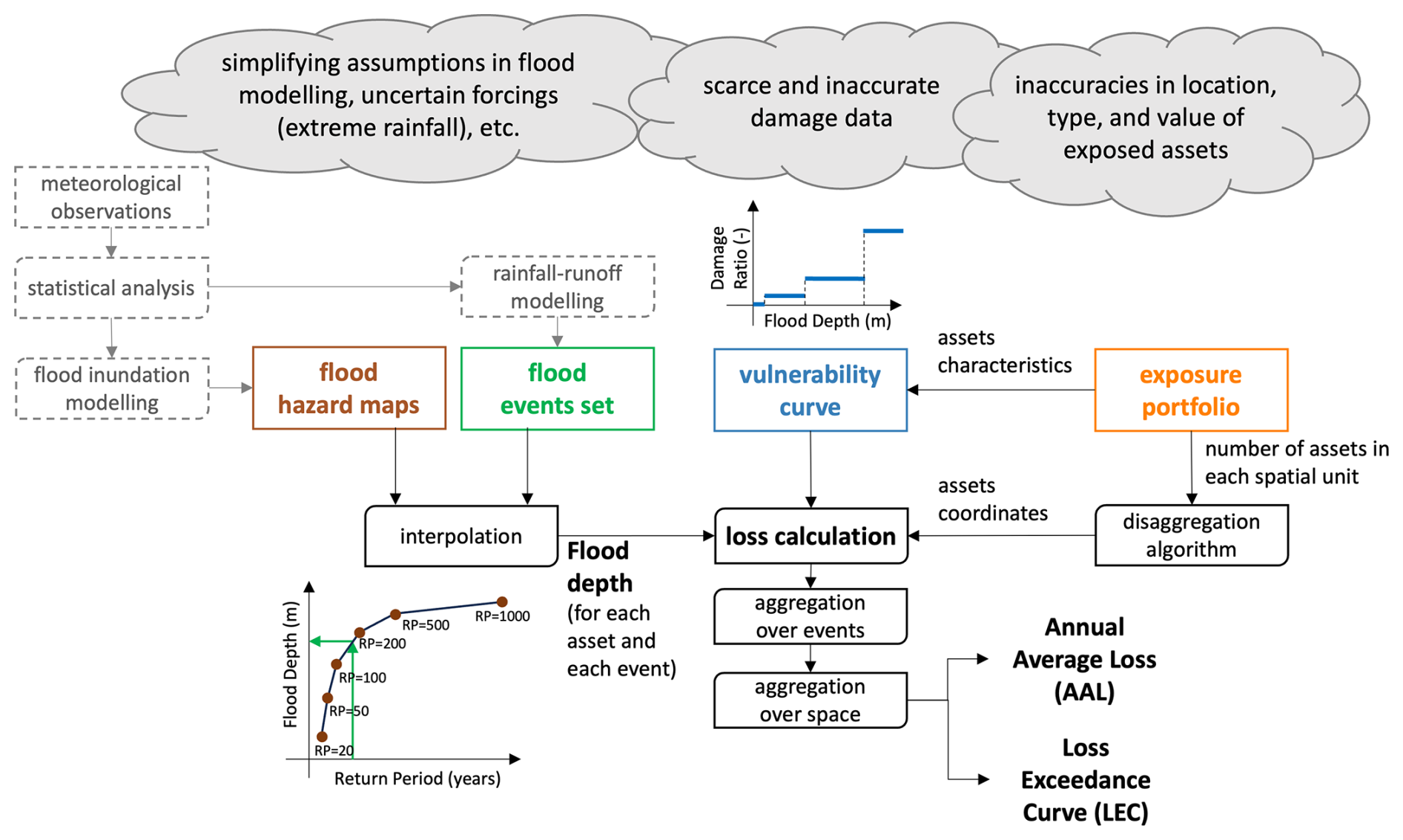
Figure 3 The typical structure of flood loss models used in the (re)insurance sector and their main sources of uncertainty. Coloured boxes highlight the level in the modelling chain where we will apply input variations in our “backward-from-the-end” Global Sensitivity Analysis (see Sect. 4.1).

Vulnerability curve. The flood depth at each location and for each flood event (FD_s,k) is then used to calculate the damage ratio through a vulnerability curve (DR(⋅) in Eq. 1). Several different curves have been developed in different countries and for different applications – for a review and comparison see e.g. Jongman et al. (2012) or Cammerer et al. (2013). In the two applications presented here, we will employ step functions (see Fig. 3), which corresponds to assuming that sufficiently similar flood depths all lead to the same damage ratio. Note that the lower bound of the first step where DR>0 represents the height at which water can enter a building (the threshold height of the property) and therefore the point at which damages begin to occur. The depth values at which this and the subsequent steps start, and corresponding damage ratios, vary depending on building characteristics such as use (e.g. residential or commercial) and type (e.g. house, apartment, warehouse), and on coverage (e.g. buildings insurance vs. contents insurance). Vulnerability curves for the two study regions presented in Sect. 5 were developed internally by JBA starting from the functions provided in the Multi-Coloured Manual (Penning-Rowsell et al., 2014) and adjusted based on various sources of data, including loss data from past events and publicly available information such as the Geoscience Australia GAR15 report (Maqsood et al., 2014).

Exposure portfolio. Finally, the estimated damage ratio value is multiplied by the value of the exposed asset (EV_s) which is retrieved from the exposure portfolio. The exposure portfolio contains all the relevant information regarding the exposed assets (e.g. location, total value etc.). Exposure portfolios can be provided at different levels of spatial resolution. The most detailed portfolios include information about the exact location (expressed with latitude and longitude coordinates) of every asset, along with details about the building characteristics and insured value. Lower resolution portfolios include information about the total number of buildings and their “typical” characteristics within a certain spatial unit. Such spatial unit can be a CRESTA zone or a province or, in the case of most aggregate portfolios, an entire country. The model then applies a disaggregation algorithm to locate the assets in each spatial unit based on other higher-resolution data (typically population density). The exposure portfolios used in the two case study applications will be briefly described in Sect. 5.

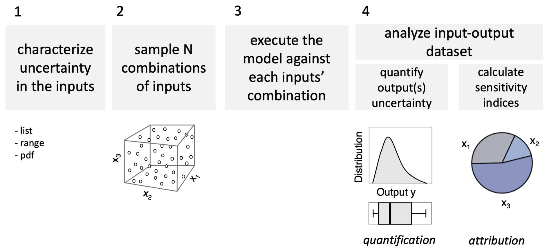
Figure 4 The steps of global sensitivity analysis for the quantification and attribution of uncertainty in model output(s).

3 The global sensitivity analysis (GSA) approach

GSA is a methodology to systematically investigate how variations in the inputs of a model (including parameters, forcing inputs, or initial conditions) propagate into variations in the model outputs.

In brief, GSA comprises four key steps (Fig. 4). First, the analyst selects the uncertain model inputs that will be subject to the analysis and characterizes their uncertainty. Note that uncertain inputs can be both numerical, such as forcing data and parameters, and categorical, such as discrete modelling choices and assumptions. Second, a prescribed number of input combinations are generated through statistical sampling (e.g. random sampling or Latin hypercube sampling) from the input distributions defined in the first step. For categorical inputs, a discrete uniform distribution can be used for sampling. Third, the model is run for each input combination, and one or more output metrics are calculated for simulation. Here, the output metrics are the average annual loss and the loss exceeded with given probabilities of Eqs. (2) and (3). Fourth, the input–output dataset is analysed to quantify the uncertainty in the output metrics, e.g. in the form of a frequency distribution or a set of quantiles, and to quantify the relative contribution of the uncertain inputs to the output uncertainty, e.g. in the form of sensitivity indices. Sensitivity indices typically vary between 0 and 1, with higher values denoting greater contribution to output uncertainty.

The definition of the sensitivity indices, and the calculation procedure to approximate their values from the input–output dataset, vary depending on the chosen GSA method. For example, some methods use correlations between inputs and output samples to measure sensitivity, while other methods measure sensitivity to an input through the reduction in output variance (or some other statistic) when fixing that input. More details about different GSA methods and the implementation of the above four steps can be found in, e.g. Saltelli et al. (2007) and Pianosi et al. (2016).

4 Challenges in applying GSA to large-scale flood loss models and possible solutions

When applying GSA to a complex flood risk model like the one described in Sect. 2, several challenges arise. In the following sections, we discuss these challenges and possible ways forward, which are then demonstrated in our example application.

4.1 Reducing the number of input uncertainties

The first challenge in the application of GSA to a complex modelling chain like that underpinning a flood risk model is that the number of input uncertainties that could be propagated and analysed is potentially very large. This is problematic as it increases the analytical burden of characterising input uncertainties (step 1 in Fig. 2) and the computational burden of executing the model (step 3), as the number of input combinations required to approximate sensitivity indices grows quickly with the number of uncertain inputs (Sarrazin et al., 2016).

To overcome this challenge, here we suggest that instead of propagating all possible uncertainties “forward-from-the-start” of the modelling chain, one can follow a structural dimension reduction through a “backward-from-the-end” approach and perturb only the inputs to the last component of the modelling chain, that is, the loss calculation (Fig. 3). By doing so one only has four input uncertainties: (i) the flood hazard maps used for interpolation of flood depths (FD_s,k in Eq. 1); (ii) the event set; (iii) the vulnerability curve DR(⋅); and (iv) the exposed assets value EV_s.

Framing the GSA in this way makes it computationally tractable while still fulfilling the key aim of determining the dominant control of the uncertainty in the flood losses. Once this has been established, the root causes can be further analysed, if needed, by going “one step up” the modelling chain and conducting a new GSA of the model component responsible for the dominant uncertainty. In other words, the idea is that instead of trying to conduct one comprehensive analysis of the entire modelling chain, which may be computationally intractable, one could start with a smaller analysis of the end of the modelling chain and use the results to focus subsequent rounds of equally tractable analyses on the components that have been proven to matter most.

4.2 Generating physically-plausible input samples

Having embraced a “backward-from-the-end” approach, a subsequent challenge is how to produce random yet physically plausible samples for complex spatially distributed input uncertainties such as flood hazard maps. For example, perturbing flood depths at individual locations independently from one another may produce physically implausible hazard maps, while defining spatially consistent perturbation is possible in principle but difficult in practice.

One approach to maintain spatial consistency could be to put together a set of hazard maps produced by different inundation models (or models with different set-up choices) and randomly sample from this set with uniform discrete probability (i.e. where each possible choice gets the same probability of being sampled). A similar idea has been used in the context of heatwaves rather than flood risk assessment (Dawkins et al., 2023).

A second option, which we will use in the Rhine River Basin application of Sect. 5.1, is to exploit the fact that each hazard map and flood event in the event set is associated with a return period (see Sect. 2) and thus randomly sampling the return period leads to retrieving a different map/event and thus producing different flood depths for each model execution, while maintaining spatial consistency over the simulated domain.

A third option to perturb flood depths consistently across the spatial domain, which we will use in the Queensland application (Sect. 5.2), is to specify a distribution F_s(⋅) for the flood depth at each location, then generate one perturbation factor (p) via uniform sampling over [0,1], and finally obtain a perturbed flood depth at each location by inversion of the cumulative location-specific flood depth distribution: FD${}_s=F_s^{-\mathrm{1}}\left(p\right)$.

4.3 Characterising poorly bounded input uncertainties

Another challenge in applying GSA to large-scale loss models is the characterisation of the selected input uncertainties. In fact, the scarce quantity and quality of data on, for example, extreme floods and flood damages, makes it difficult to rigorously specify probability distributions for most input uncertainties (Apel et al., 2004). This is critical as obviously the results of the GSA – i.e. the relative importance attributed to every input uncertainty – strongly depend on the chosen distributions (e.g. Paleari and Confalonieri, 2016).

To handle this problem, we propose to conceptualise the probability distributions of the inputs not as statements of what is likely, but rather as statements of what cannot be excluded. In practice, this means using uniform distributions with very wide ranges: the choice of uniform distributions translates our inability to discriminate between probabilities of different input values; the use of wide ranges allows for testing input values that may be largely different from “default” set-up, but still physically plausible.

One can then perform a “sensitivity analysis of the sensitivity analysis” and investigate how sensitivity results are affected by the ranges' definition. For example, one could reduce the range of the input that was found to be dominant and check by how much that range needs reducing before the input stops being dominant. In other words, instead of asking: “what is the relative importance of input X given its (assumed) uncertainty distribution?” one can ask: “how much do we need to reduce uncertainty in input X before it becomes unimportant (or another input becomes more important)?”

4.4 Reducing the number of model executions

The last challenge is that of keeping the overall computational burden of the analysis within the limits of available resources. While continuous increase in computing power may ease this problem in the long-term, the requirement of executing the model hundreds or potentially thousands of times for the forward propagation of input uncertainties (step 3 in Fig. 4) remains a bottleneck to the application of GSA to large-scale flood loss models.

One way to mitigate the issue is to use a GSA method as frugal as possible, such as the method of Morris (1991), or to use a surrogate modelling approach such as polynomial chaos expansion (Sudret, 2008). Here, we use the PAWN method (Pianosi and Wagener, 2015) which has been shown to effectively estimate sensitivity indices with a relatively low number of model evaluations (Pianosi and Wagener, 2018). Another advantage of PAWN is that, unlike the method of Morris and surrogate modelling approaches, it is applicable also when some of the inputs are categorical, as will be the case in the Queensland application. With this method, the sensitivity of the output y to the input factor x_i is quantified by measuring the distance between the unconditional cumulative distribution function (CDF) of y that is obtained by varying all inputs simultaneously, and the conditional CDF obtained when all inputs vary but x_i. Operationally, given the input-output samples dataset, the PAWN sensitivity indices $\widehat{S_i}$ are approximated by splitting the range of variation of each input uncertainty x_i into n equally-spaced intervals I_k, using

$$\begin{array}{}\text{(5)}& {\displaystyle }{\widehat{S}}_i={\text{mean}}_{k=\mathrm{1},\mathrm{\dots },n}\text{KS}\left(I_k\right),\text{(6)}& {\displaystyle }\text{KS}\left(I_k\right)=\underset{y}{max}\left|{\widehat{F}}_y\right(y)-{\widehat{F}}_{y\mathrm{|}{x}_i}(y\mathrm{|}{x}_i\in I_k\left)\right|,\end{array}$$

where ${\widehat{F}}_y\left(y\right)$ and ${\widehat{F}}_{y\mathrm{|}{x}_i}(y\mathrm{|}{x}_i\in I_k)$ are the unconditional and conditional CDFs of the output y and KS is the Kolmogorov–Smirnov statistic that measures the distance between the CDFs. If the input x_i is categorical, splitting into intervals is not required and the conditional CDFs are simply calculated for each categorical value c_k of the input, i.e. ${\widehat{F}}_{y\mathrm{|}{x}_i}(y\mathrm{|}{x}_i=c_k)$. The PAWN sensitivity indices vary between 0 and 1: the higher the value of the sensitivity index the more sensitive the output to the input uncertainty. The code to implement PAWN in Matlab, R and Python is available in the SAFE Toolbox (Pianosi et al., 2015).

To further reduce the number of model evaluations required by the GSA, we also propose a simple bootstrap-based approach to robustly determine the dominant uncertainty even if using a particularly small sample size. With this approach, the calculation of the PAWN sensitivity indices is repeated for a prescribed number of times using bootstrap resamples of the original input-output dataset. For each bootstrap resample, the dominant input uncertainty is identified as the one with highest sensitivity index. Then, for each input uncertainty, we can calculate the frequency with which it was identified as dominant across bootstrap resamples. Last, input uncertainties are ranked in order of decreasing frequency of being dominant. If the input uncertainty with highest frequency exceeded the second highest by at least a prescribed difference (0.3 in our case), we deem that input uncertainty as dominant. If instead the difference between the first and second highest frequencies is less than 0.3, we deem both the first and second ranked as dominant uncertainties.

The key point here is recognising that sensitivity indices are just a means to achieving the actual relevant result, which is the ranking of input uncertainties from most to least important, and that a sufficiently robust ranking can often be obtained even if indices are not precisely approximated due to the small sample size used (Sarrazin et al., 2016).

5 Application examples

In this section, we showcase some of the solutions for applying GSA to a large-scale flood loss model as described in Sect. 4, using two application examples.

The first application is the flood loss model of the Rhine River basin in Europe, covering a spatial extent of approximately 185 000 km² and including major European cities of eight different countries (Switzerland, Liechtenstein, Austria, France, Germany, Belgium, Luxembourg, and the Netherlands). An exposure portfolio was constructed at CRESTA level using market-informed values. We analysed the propagation of uncertainty in the value of residential buildings, vulnerability curves and the return period of the flood events and hazard maps, with the goal of identifying the dominant controls of uncertainty in the loss predictions across the spatial domain, and thus understand which model component – hazard, vulnerability or exposure – should be prioritized in future efforts for reducing uncertainty, and where.

The second application is the flood loss model of Queensland in Australia, covering a spatial extent of over 1 700 000 km² and including over 300 000 assets. Here, we focused on understanding to what extent the quality of the exposure portfolio matters with respect to other sources of uncertainty – including uncertainty in future climate. The motivation is that while substantial attention has been devoted to improving the hazard component of flood loss models (including incorporating climate change), exposure data may vary widely in granularity and reliability. For instance, reinsurers frequently receive aggregated portfolios from insurers, which lead to loss of critical information about building location and characteristics. To perform our analysis, we created a coordinate level portfolio informed by the PERILS Industry Exposure & Loss Database (https://www.perils.org/, last access: March 2026) and then created three more portfolios at increasing level of aggregation. We then used GSA to quantify the relative importance of using one portfolio over the other with respect to other uncertainty sources and modelling choices – including the choice between different climate-conditioned event sets.

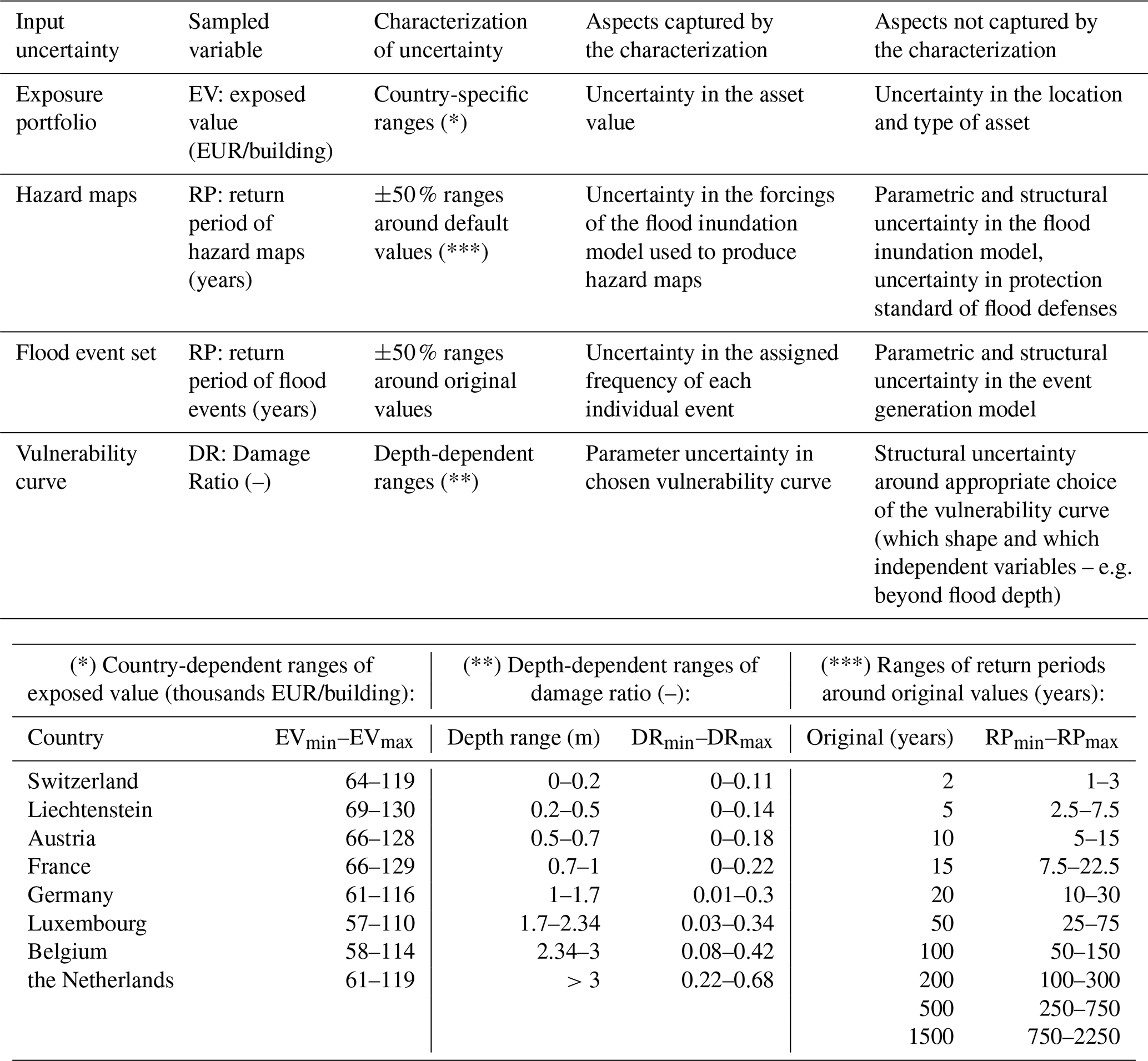
Table 1 Input uncertainties analysed in the GSA demonstration for the Rhine River basin, their characterisation and underpinning assumptions and implications.

5.1 Rhine River basin case study

To identify the minimum and maximum plausible values for each input uncertainty, we systematically reviewed the scientific literature on flood risk in the Rhine River basin and identified past studies that quantified flood return periods, depth-damage ratios and residential building values (and their possible variability) for either specific locations or sub-regions within the basin. We synthetised this information by taking the average of the minimum and maximum values found in such past studies, to obtain the uncertainty ranges for sampling reported in Table 1. A detailed description of this literature review process is reported in Sarailidis (2023, Chapter 3). In brief, ranges for the building values were based on pooling together data reported in nine previous studies and identifying minimum and maximum reported values for each country in the basin. For the flood return periods, we found five studies which however provided uncertainty ranges at two gauging stations only (Cologne and Lobith). In the lack of other information, we arbitrarily decided to apply ±50 % ranges around the default return period values. Note that this approach provides ranges relatively consistent with those derived from literature at Cologne and Lobith stations (see Table 4.1 in Sarailidis, 2023) although there is no further evidence to back up the choice elsewhere. Finally, for the damage ratio of the vulnerability curves, we pooled together data from eight studies which used different vulnerability curves, and not only step functions, possibly leading to overestimating the uncertainty associated to this parameter alone. As discussed in Sect. 4.2 and 4.3, the definition of uncertainty ranges is one of the most difficult steps in the application of GSA, as data to inform this choice are often missing or sparse. This is why it will be important to analyse the impact of these choices on key sensitivity results, as we will show with an example later on.

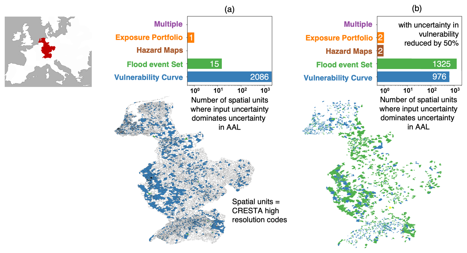
Figure 5 Example results of a global sensitivity analysis of the Rhine River Basin showing dominant input uncertainties for average annual loss across the spatial domain for (a) original uncertainty ranges as in Table 1 (authors' re-elaboration of results in Sarailidis, 2023) and (b) reduced uncertainty ranges for the vulnerability curves.

We then used Latin hypercube sampling to generate 400 combinations of the 4 uncertain inputs and executed the model against each of these input combinations. Sensitivity indices were calculated using the PAWN method and dominant input uncertainties identified with the bootstrapping-based approach described in Sect. 4.3.

Figure 5 shows an example of the type of results that can be produced by the GSA. The map on the left shows the Rhine River basin with spatial units (high resolution CRESTA zones) coloured according to the dominant input uncertainty on average annual loss (AAL) in that units (units coloured in white did not include any exposed assets). The bar plot summarises the total number of units in which each input uncertainty is dominant for AAL estimation. It shows that damage ratio is the dominant uncertainty almost everywhere across the spatial domain. This result aligns with previous sensitivity analyses of flood loss models for smaller regions of the Rhine River basin (e.g. De Moel et al., 2014; Metin et al., 2018) as well as an industry report containing opinions of practitioners (Lighthill Risk Network, 2019) that identified uncertainty in the vulnerability component as a key contributor to uncertainty in AAL estimates and a priority to improve precision of flood loss estimates. On the other hand, as mentioned before, the uncertainty ranges of the damage ratios underpinning this result are particularly wide as they envelope damage ratio coefficients previously used with different vulnerability curves, potentially overestimating parameter uncertainty for a given curve (the step function, in our case). As discussed in Sect. 4.3, it is therefore interesting to explore how much the choice of the uncertainty ranges affects the results. This is exemplified in the right panel in Fig. 5, which shows that the uncertainties in the vulnerability curves (i.e. the variability ranges of the damage ratios) need to be reduced by 50 % from their initial definition, in order for the second most important input uncertainty, i.e. the flood event set, to become dominant in as many spatial units. This suggests that the overall sensitivity analysis is, in this case, tolerably robust to the assumptions made about the damage ratio uncertainties.

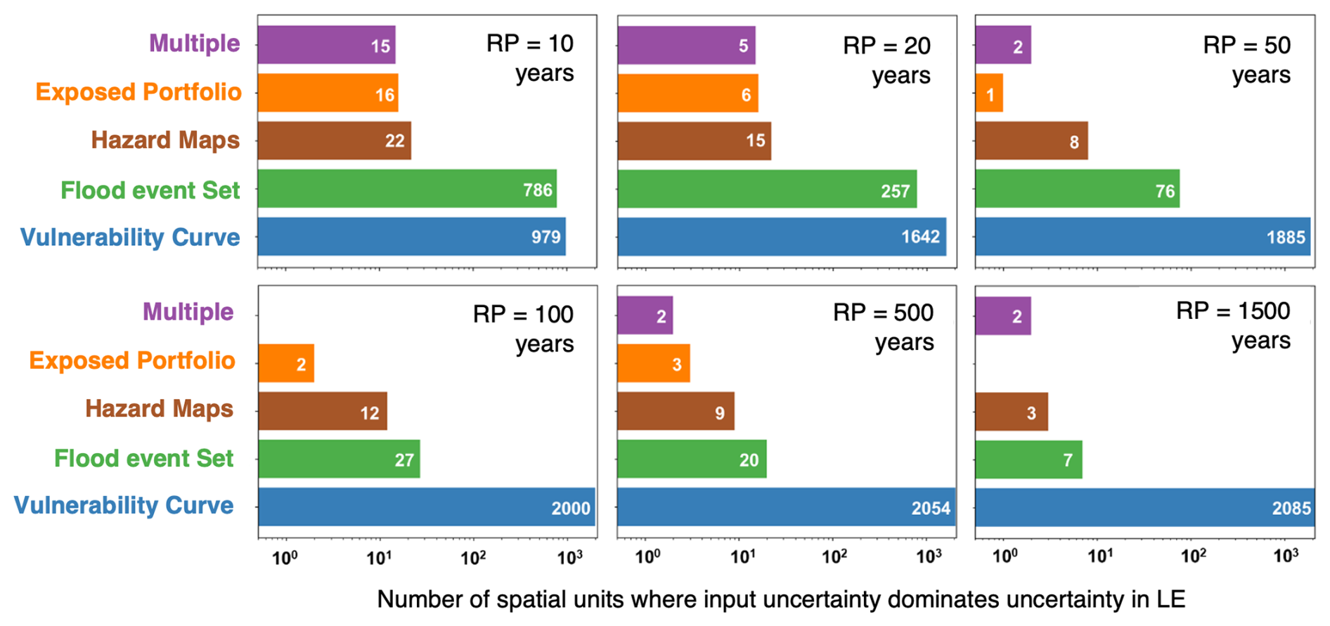
Figure 6 Example results of a global sensitivity analysis of the Rhine River basin showing dominant input uncertainties on loss exceeded (LE) with different return periods (RPs) (authors' re-elaboration of results in Sarailidis, 2023).

Figure 6 shows the dominant input uncertainties for another output metric typically used by (re)insurers: the loss exceeded (LE) with six different return periods. It shows that, for small return periods (RP =10 years or 20 years), the LE uncertainty is dominated by either the vulnerability curve or the event set uncertainties. At larger return periods, the vulnerability curve becomes the dominant uncertainty in more spatial units. This can be explained by the fact that losses with low return periods are produced by small and frequent flood events where the impact of localized features is greater, and thus the uncertainty in flood depths and/or individual asset value is more important. Loss levels with large return periods instead are caused by large inundations where many assets experience similar flood depths and thus flood loss uncertainty is mainly driven by the uncertainty in the damage ratios.

These findings are somewhat consistent with previous literature. For example, in their analysis of the variance of the European flood model, Kaczmarska et al. (2018) also found that the vulnerability component is increasingly important at greater return periods of exceeded losses. Local-scale studies at different reaches (e.g. Apel et al., 2008) or subbasins (Winter et al., 2018) of the Rhine River basin instead found slightly contrasting results: the former found that LE at low return period is dominated by uncertainty in frequency of flood events and the latter found that it is still dominated by uncertainty in vulnerability. It is also worth noting that in this application we did not consider the uncertainty in the flood defences dataset, which may include errors in the definition of the area benefitting from defences or in the value of the associated standards of protection (e.g. because of defence degradation). As this source of uncertainty can have a large influence on flood hazard mapping (e.g. Vousdoukas et al., 2018; Paprotny et al., 2025) its exclusion from the GSA may have led us to underestimate the role of hazard uncertainty in this application.

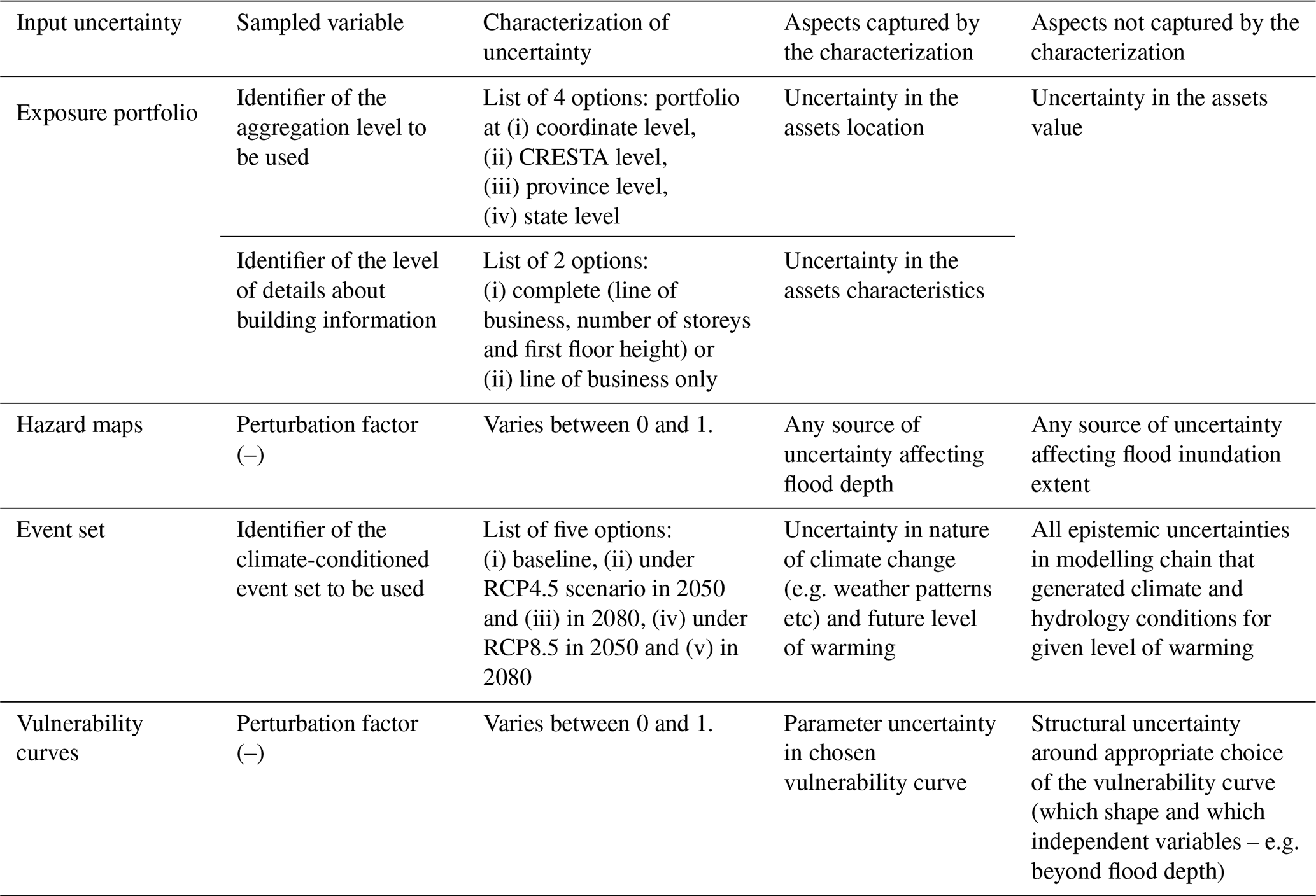
Table 2 Input uncertainties analysed in the GSA demonstration for Queensland, their characterisation and underpinning assumptions and implications.

5.2 Queensland case study

Table 2 describes the input uncertainties considered in the Queensland case study. Similarly to the Rhine River basin case study, we considered uncertainties in the vulnerability curve parameters and in the hazard maps (though this time using a different approach to perturbing the flood depths – see Table 2 and Sect. 4.2). The key differences with the previous case studies are two. First, for the event set, we do not perturb the characteristics (e.g. return periods) of the events in one set, but we sample from five different sets, each one built under a different climate change scenario. Second, for the exposure portfolio, again we do not perturb characteristics (e.g. building value) of the assets in one portfolio but we sample from different portfolios built through intersecting two different characteristics: the level of spatial aggregation (from low to high we consider: coordinate level, CRESTA, province, and state level) and the level of detail of the building characteristics (we consider two cases: complete information including the line of business, number of storeys and height of first floor for each building, and a partial information including the line of business only). These portfolios are representative of different levels of information that may be accessible to different users of flood loss models in the risk analysis sector. For example, insurers might have coordinate-level portfolios of their clients, whereas reinsurers may only have access to CRESTA-level portfolios, and an international risk reduction agency may only have access to a province-level or even state-level portfolios.

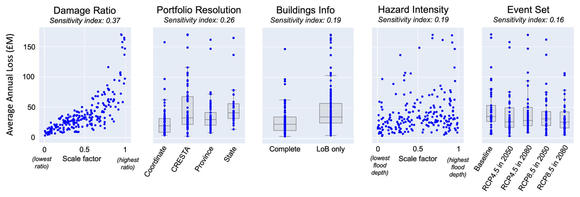
Figure 7 Example results of a global sensitivity analysis of the flood loss model for Queensland, Australia showing scatter plots of model output (average annual loss, AAL) against the five input uncertainties. For discrete inputs, box plots are overlayed to represent the 25th, median, and 75th percentile of the output sample distributions at each discrete input values. The title of each scatter plot reports the PAWN sensitivity index for each input.

Figure 7 shows an example of the type of insights delivered by the GSA. Each scatter plot shows the values of the output metric (average annual loss) against the 210 samples of each input uncertainty. The more clearly a scatter plot shows a pattern when moving along the horizontal axis, which represents the variability range of an input, the greater the influence of that input. For discrete inputs, we use boxplots to help visualise the distribution of output values for each discrete choice of input value. The damage ratio (first scatter plot from the left) is the most influential input, with a clear pattern of higher losses with increasing values of damage ratios. The strength of such input–output relationship is confirmed by the value of the PAWN sensitivity index, reported at the top of the scatter plot. The second most influential input is the choice of the portfolio resolution, with more aggregate portfolio generally leading to higher losses. Predicted losses are slightly higher when the portfolio includes less building information (third scatter plot) and when hazard intensity is increased (fourth). The choice of the event set has the least influence on the loss predictions. The findings confirm the key role of uncertainty in the vulnerability component for predicted losses, consistent with results from the Rhine River basin application. They also show that the spatial resolution of the exposure portfolio has an important impact on loss estimates.

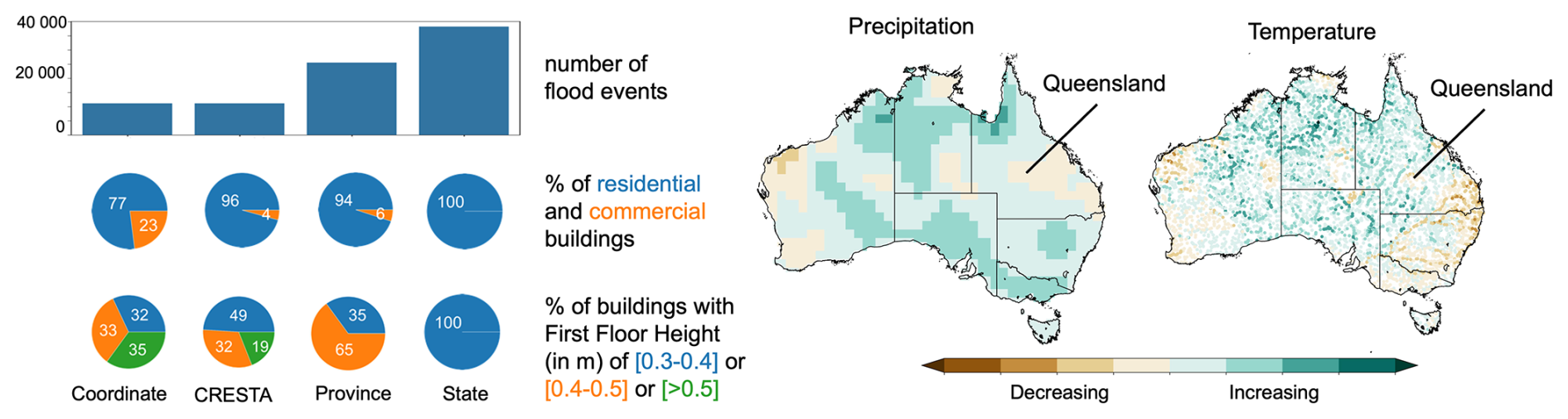
Figure 8 Exposure and building characteristics in the four portfolios considered in the GSA application in Queensland (left) and projected changes in climate and hydrology under the RCP4.5 in 2080 scenario.

In this case study, more aggregate (i.e., lower resolution) portfolios lead to overestimated losses, assuming the coordinate-level portfolio as the reference or “truth”. To understand why, we analysed the characteristics of these different portfolios and identified two key sources of systematic bias (Fig. 8 – left). First, the disaggregation algorithm spreads assets more widely than in the coordinate-level portfolio. This increases the number of assets exposed to any given flood event. Second, aggregation leads to loss of detail in building characteristics. In each spatial unit of an aggregated portfolio, all assets are assigned the same characteristics. This tends to increase the attributed vulnerability relative to the coordinate-level portfolio. For example, in the coordinate-level portfolio, 77 % of the buildings are residential and therefore classified as more vulnerable than the 23 % commercial ones. In contrast, the residential portion is 96 % in the CRESTA-level portfolio, 94 % at the province level, and 100 % at the state-level. Similar patterns are seen in floor height data. In the coordinate-level portfolio, 32 % of the buildings have a first-floor height below 0.4 m – a characteristic associated with higher vulnerability. This increases to 49 % in the CRESTA-level portfolio and 100 % in the state-level one. Conversely, buildings with first floor height above 0.5 m – a characteristic associated with lower vulnerability – decline from 35 % in the coordinate-level portfolio to 19 % at the CRESTA-level, and 0 % at the province and state levels. In summary, the disaggregation algorithm introduces systematic bias in both exposure and vulnerability when moving from detailed to aggregate exposure portfolios.

Figure 7 also suggests a very limited role of future climate uncertainty with respect to other sources of uncertainty. This may be explained by the fact that the climate projections used here suggest both increasing and decreasing trends in precipitation and river flows in different sub-regions of Queensland (Fig. 8), and therefore these opposite trends may offset each other when looking at overall losses across the region. Here, the flood event sets were generated based on the outputs of a single climate model, MRI-ESM2-0 (Yukimoto et al., 2019), and incorporating event sets generated from other models could capture a wider range of uncertainty.

6 Outlook and Conclusions

This paper has discussed challenges and possible ways forward in the application of global sensitivity analysis to flood loss models across large spatial domains. We have discussed and demonstrated several strategies to make GSA tractable even for computationally expensive models such as large-scale flood loss models. Thanks to these strategies, we were able to extract meaningful information from Monte Carlo simulations based on a few hundred model runs. Still, given the large spatial domain covered, these runs required up to 3 d to run on relatively powerful machines: the computational facilities of the Advanced Computing Research Centre at the University of Bristol for the Rhine River basin application, and JBA's machine (an Intel i7 3.4 GHz, with 16 cores, and 128 GB RAM) for the Queensland application.

The two example applications reported here, to the Rhine River basin in Europe and Queensland state in Australia, consistently signal that uncertainty in the quantification of vulnerability is the dominant source of uncertainty in our flood loss estimates, within the scope of the input space studied. In the Rhine River basin application, the second most important source of uncertainty (of those analysed) was the frequency of floods in the event sets. In the Queensland case study, we also found systematic biases induced by the loss of information when moving to more aggregate and less detailed exposure portfolios. These insights could be useful for model developers to set priorities for future acquisition of higher-quality data or refinement of model components; or they can be leveraged by model users – for instance in (re)insurance – to advocate for access to higher resolution exposure data.

Our sensitivity results are conditional on the choices made in the experimental design, and in particular which input variables were varied and within which ranges. Indeed, our experience suggests that the selection of the input uncertainties and their characterisation is a critical step, if not the most critical, in the application of GSA to flood loss models. For example, the choice of not including uncertainty in flood protection standard in our analysis may have led us to underestimate the importance of hazard uncertainty. In future GSA applications, this source of uncertainty could be included, for example, by allowing for flood protection standards to be randomly reduced to account for likely overestimation in commonly used datasets (Paprotny et al., 2025). As for the characterisation of the selected input uncertainties, here we used a mix of literature review and expert opinion to define their distributions. Structured approaches to elicit probabilities from experts could be very useful in this context – see O'Hagan et al. (2006) for a review of methods and e.g. Lamb et al. (2017) or Lenton et al. (2008) for application examples to bridge scour and climate risk assessments. More research on this possibly-overlooked aspect of uncertainty and sensitivity analysis will certainly be needed in the future, as also advocated by Lo Piano et al. (2022) and Page et al. (2023). Still, a degree of subjectivity in the definition of input uncertainties' distributions (or ranges) is unavoidable and therefore GSA results should always be interpreted as answers to the relative question “what are the controls of model outputs if these inputs are varied according to these distributions (within these ranges)?” At a minimum, GSA results should always be presented along with a clear summary of the key assumptions made in characterising input distributions, clarifying what sources of uncertainty are being captured and what are left out – as we did for example in Tables 1 and 2 of this paper.

Equally important in the communication of GSA results is to be clear about the fact that, being a stress test of the model, not of the system being modelled, GSA can only tell us about the behaviour of the model within the scope of its underpinning assumptions, and not whether those assumptions are correct. Put differently, and returning to the distinction made in Fig. 1 – GSA can help to tackle the precision of the model but not its accuracy. For example, we have found that reducing uncertainty in damage curves would be of paramount importance in making the loss predictions more precise in the Rhine River case study, but this does not imply it would make them more accurate if the use of mean damage ratios oversimplifies the reality of damage distributions and other variables beyond flood depth would be needed to better predict damage (Lighthill Risk Network, 2019; Wing et al., 2020).

Overall, GSA can, and we think should, play an essential role in the diagnostic evaluation of models (Wagener et al., 2022) and in guiding investments towards improving data quality and model components where they will have the greatest effect. We hope this paper will provide motivation as well as practical ideas to foster the application of GSA to flood risk models also when they cover large spatial domains, and contribute to increasing their transparency and legitimacy.