Quantifying fire effects on debris flow runout using a morphodynamic model and stochastic surrogates

Fire affects soil and vegetation, which in turn can promote the initiation and growth of runoff-generated debris flows in steep watersheds. Postfire hazard assessments often focus on identifying the most likely watersheds to produce debris flows, quantifying rainfall intensity-duration thresholds for debris flow initiation, and estimating the volume of potential debris flows. This work seeks to expand on such analyses and forecast downstream debris flow runout and peak flow depth. Here, we report on a high-fidelity computational framework that enables debris flow simulation over two watersheds and the downstream alluvial fan, although at significant computational cost. We then develop a Gaussian Process surrogate model, allowing for rapid prediction of simulator outputs for untested scenarios. With a modest training of debris flow simulations, this surrogate is able to approximate peak flow depth with a mean squared error that is generally in the range of 0.1–0.2 m. We utilize this framework to explore model sensitivity to rainfall intensity and sediment availability as well as parameters associated with saturated hydraulic conductivity, hydraulic roughness, grain size, and sediment entrainment. Simulation results are most sensitive to hydraulic roughness and grain size. Further, we use this approach to examine variations in debris flow inundation patterns at different stages of postfire recovery, and we find that the area inundated by postfire flows decreases substantially over a time period as short as 9 months. In this case, we also see that temporal changes in hydraulic roughness and grain size following fire would be particularly beneficial for forecasting debris flow runout throughout the postfire recovery period. The emulator methodology presented here also provides a means to compute the probability of a debris flow inundating a specific downstream region, consequent to a forecast or design rainstorm. This workflow could be employed in prefire scenario-based planning or postfire hazard assessments.

1 Introduction

Fire alters soil and vegetation, leading to increases in runoff and erosion (McGuire et al., 2024; Moody et al., 2013). In extreme cases, particularly when steep watersheds burn at moderate or high severity, rapid entrainment of sediment into runoff can produce debris flows (Kean et al., 2011; Gabet and Bookter, 2008; Esposito et al., 2023; Conedera et al., 2003; Nyman et al., 2011; Diakakis et al., 2023). Postfire debris flows generated by runoff are most common in the first year following fire, when fire-driven reductions in soil infiltration capacity, rainfall interception, and hydraulic roughness are most extreme (DeGraff et al., 2015; Hoch et al., 2021; Thomas et al., 2021; Esposito et al., 2023; Graber et al., 2023). Due to the complex interactions among runoff, sediment transport, and debris-flow initiation and runout following fire, mathematical models that couple these processes have the potential to inform our understanding of the magnitude and downstream effects of postfire debris flows, including how they change through time as landscapes recover (McGuire et al., 2021). Postfire debris flows can drive sediment yields that are orders of magnitude above background rates (Nyman et al., 2015) and provide an important link between hillslopes, channels, and fans in the postfire sediment cascade (McGuire et al., 2024). Predictions of the size and travel distance of postfire debris flows are therefore beneficial for hazard assessments as well as our more general understanding of landscape evolution in fire-prone regions (Orem and Pelletier, 2016; Struble et al., 2023).

The exploration of postfire debris flow processes through application of morphodynamic models for runoff and sediment transport, however, is often limited by the high dimensionality, poor constraints on parameters, and substantial computation time of the models. Quantification of uncertainties associated with model parameters, and incorporation of those uncertainties in probabilistic predictions of hazard, often require use of simulation ensembles with hundreds or thousands of members, greatly increasing computational costs (Bayarri et al., 2015). In this work, we accelerate a recently developed morphodynamic model of runoff and sediment transport (McGuire et al., 2017), and pair model runs with stochastic surrogates for high-dimensional output (Gu and Berger, 2016) as a strategy for simulating the initiation, growth, and runout of postfire debris-flows. This acceleration also enables us to rapidly explore rainfall intensity and fire effects on soil and vegetation, including how they change with time since fire, debris flow runout and inundation patterns.

The processes leading to the initiation and growth of postfire runoff-generated debris flows involve the generation of spatially-distributed, infiltration-excess overland flow and its subsequent interaction with sediment on hillslopes and in channels (Santi et al., 2008; Staley et al., 2014; McGuire et al., 2017; Guilinger et al., 2020). This presents a contrast to debris flows that mobilize from shallow landslides, which initiate when infiltration promotes increases in pore-water pressure that causes a discrete mass of soil to become unstable on a hillslope (Iverson et al., 1997). The source of sediment for postfire runoff-generated debris flows can come from a combination of processes, including widespread, shallow erosion on hillslopes in response to raindrop-driven sediment transport and unconfined sheet flow, rill erosion on hillslopes in areas of concentrated flow, and channel scour (Santi et al., 2008; Staley et al., 2014; McGuire et al., 2017; Tang et al., 2019). All three processes are more efficient at eroding sediment following fire as a result of decreases in ground cover and increases in runoff (Robichaud et al., 2016), particularly rill and channel erosion processes where overland flow does the work to entrain and transport sediment (Sheridan et al., 2007; Wagenbrenner et al., 2010). In areas of unconfined, shallow flow, raindrops facilitate sediment detachment and transport in combination with runoff (Kinnell, 2005). Raindrop-driven sediment transport on hillslopes increases following fire due to removal of the vegetation canopy, litter, and duff, that tend to shield the soil surface from raindrop impact in unburned settings.

Models designed to simulate runoff-generated debris flows from initiation to deposition must therefore account for spatially distributed runoff and sediment transport as well as changes in flow behavior resulting from spatial and temporal variations in sediment concentration. Fully developed debris flows are characterized by volumetric sediment concentrations in excess of 40 %–50  %, though they initiate from runoff with initially negligible sediment concentration. Postfire runoff-generated debris flows initiate in response to short-duration bursts of high intensity rainfall (Kean et al., 2011). Rainfall intensity averaged over a 15 min time period, I₁₅, is correlated well with runoff magnitude at the outlet of small, recently burned watersheds. Moreover, threshold values of I₁₅ have proven to be reasonable predictors for debris flow initiation in the western USA (Kean et al., 2011; Staley et al., 2017). Rainstorms that contain multiple, distinct bursts of high intensity rainfall, such as where I₁₅ exceeds the debris flow threshold multiple times in a single event, can lead to multiple pulses of debris flow activity (Kean et al., 2011). One benefit of morphodynamic models that are capable of simulating the debris-flow lifecycle from initiation to runout is their ability to directly account for the effects of temporally varying rainfall intensity on debris flow processes, including the formation of distinct debris flow surges and their influence on inundation extent. In contrast, models designed only to simulate debris flow runout processes (i.e. neglecting runoff and sediment transport), can be employed by defining an inflow hydrograph above the anticipated runout zone based on a runoff hydrograph and an estimated debris flow volume, or by allowing a pile of sediment and water to flow downstream from a pre-defined initiation zone (Barnhart et al., 2021; Gorr et al., 2022; Gibson et al., 2022). As a result, employing morphodynamic models to estimate debris flow runout avoids introducing epistemic uncertainty related to specifying a volume of material associated with an inflow hydrograph.

McGuire et al. (2017) developed a model that accounts for infiltration, runoff, sediment transport, and changes to flow resistance driven by sediment concentration in order to simulate postfire debris flow initiation and growth. In this model, rainfall drives sediment entrainment and transport processes that naturally lead to debris flow initiation when hydrogeomorphic conditions give rise to flows with sufficiently high sediment concentrations. Since rainfall, runoff, and erosion processes are related to model parameters known to change following fire, such as saturated hydraulic conductivity (Perkins et al., 2022; Ebel et al., 2022; Thomas et al., 2021), hydraulic roughness (Stoof et al., 2015), and vegetation cover (Stoof et al., 2012), this framework can be used to explore how postfire recovery affects debris-flow initiation, growth, and runout. The model is computationally intensive, especially when simulating debris flow initiation and runout processes over large areas, and contains a number of parameters that are challenging to constrain (McGuire et al., 2016, 2017). Thus far, model applications have been limited to examining debris-flow initiation processes in small headwater basins (<0.2 km²) where prior work and intensive field monitoring helped constrain parameter values (McGuire et al., 2021, 2017; Tang et al., 2019). Here, we employ adaptive mesh refinement and parallel computations through the Titan framework (Patra et al., 2005; Dalbey et al., 2008) to make model application more tractable over larger spatial domains, specifically with the goal of simulating the entirety of the postfire debris-flow lifecycle from runoff generation and debris flow growth to runout. In addition, we employ statistical emulators trained on well-chosen simulation ensembles, for fast approximations to solutions of the model equations, to explore the influence of model parameters on debris-flow runout extent and the temporal persistence of debris flow hazards after fire.

Gaussian process emulators (GPs) are a powerful class of statistical surrogates that enable rapid approximation and uncertainty quantification of computationally intensive first principles (conservation laws) based models or, simulators (Currin et al., 1988; Sacks et al., 1989b; Welch et al., 1992). In the context of postfire debris-flows, GPs offer a mechanism to quickly explore spatial patterns in peak flow depth and area inundated for various parameter settings. GPs also allow for uncertainty quantification via Monte Carlo (MC) simulations of flow inundation. Along the way, GPs offer an approximate sensitivity analysis of physical parameters' effects on debris-flow inundation. Parallel partial emulation (PPE) (Gu and Berger, 2016) extends the GP methodology to field-valued outputs – in our case, flow depth at each map point (pixel). Some recent studies use PPE for flow model sensitivity analysis and calibration (Zhao et al., 2021; Zhao and Kowalski, 2022). In this work, we apply PPE to explore the effects of rainfall intensity and sediment availability as well as parameters associated with saturated hydraulic conductivity, hydraulic roughness, grain size, and sediment entrainment on peak debris flow depth and inundation extent.

Figure 1 (a) The Thomas Fire ignited on 4 December 2017 and burned over 1140 km² in southern California, USA. (b) The western portion of the burned area included a series of steep watersheds (black rectangle) above the community of Montecito, located near Santa Barbara. (c) Our study focuses on two watersheds, Oak Creek (0.45 km²) and San Ysidro Creek (7.6 km²), located upstream of Montecito. The KTYD gauge is located approximately 5 km west of the watershed centroid.

2 Study Area

The Thomas Fire ignited in December 2017 and burned more than 1100 km², including a series of steep watersheds in the Santa Ynez Mountains above the community of Montecito, USA (Fig. 1a).

On 9 January 2018, widespread rainfall developed over the burned area in association with an atmospheric river (Oakley et al., 2018). A narrow cold frontal rainband (NCFR), a relatively small-scale feature characterized by a band of intense precipitation that forms along a cold front, moved over burned watersheds above Montecito and produced a short-duration burst of intense rainfall. Peak 15 min rainfall intensities, I₁₅, in this area ranged from approximately 78 to 105 mm h⁻¹ (Kean et al., 2019). During this time period, rainfall intensities greatly exceeded the infiltration capacity of the soil, leading to infiltration-excess overland flow that generated rills on steep hillslopes (Alessio et al., 2021). The combination of intense hillslope erosion and channel incision led to runoff-generated debris flows that traveled across the populated alluvial fan (Kean et al., 2019; Morell et al., 2021; Alessio et al., 2021). The debris flows that initiated in six watersheds above Montecito mobilized more than 630 000 m³ of sediment and led to 23 fatalities, 408 damaged structures, and more than USD 1 billion in damage (Kean et al., 2019; Lancaster et al., 2021). In this study, we focus on modeling debris flow initiation, growth, and runout for two of these watersheds, Oak Creek and San Ysidro Creek. These watersheds are well suited for our study since high resolution topographic and rainfall data are available and we can leverage data collection following the fire (Kean et al., 2019) and previous work in the Transverse Ranges of southern California (McGuire et al., 2016, 2021; Tang et al., 2019; McGuire et al., 2017) to constrain model parameter ranges. In addition, the model domain, which includes the watersheds and downstream alluvial fan, is large enough to make physics-based simulations computationally challenging (Fig. 1c).

Roughly 85 % of San Ysidro Creek, which has a total drainage area of 7.6 km², burned at moderate or high severity (Fig. 1c). Approximately 49 % of Oak Creek, which is substantially smaller at 0.45 km², burned at moderate or high severity. Both the San Ysidro and Oak Creek watersheds are steep, with median slopes of 28 and 21°, respectively. The debris flows that initiated in San Ysidro Creek and Oak Creek mobilized a total volume of 307 000 m³ and inundated an area of 1 007 000 m² (Kean et al., 2019) (Fig. 1c). The grain size distribution in the debris flows was bimodal, consisting of a sandy matrix that suspended boulders with a large axis greater than several meters (Kean et al., 2019). Sediment from burned hillslopes likely supplied a substantial fraction of the sediment contained in the debris-flow matrix, which had a median grain diameter of approximately 0.1–0.3 mm (Kean et al., 2019).

3 Methodology

3.1 Simulating runoff-generated debris flows with Titan2D

Steep watersheds recently burned by fire often experience greater amounts of runoff and increased rates of sediment transport. Factors affecting rates of sediment transport, and also the initiation and growth of runoff-generated debris flows, include rainfall intensity and duration, vegetation cover, soil infiltration capacity, and sediment characteristics (e.g. grain size, erodibility). The model developed by McGuire et al. (2017) represents rainfall, infiltration, fluid flow, and sediment entrainment and deposition processes, which makes it a useful framework for simulating runoff-generated debris flows in steep terrain (McGuire et al., 2017; Tang et al., 2020). The model couples fluid flow, entrainment and deposition processes, and topographic change, such that the topography can evolve during a rainstorm in response to flow. We provide a brief overview of the governing equations, which we solve within the Titan2D framework (Patra et al., 2005; Simakov et al., 2019).

The Titan2D code employs an adaptive mesh, finite volume scheme to solve hyperbolic PDEs describing shallow-water like mass flows over digital elevation models of real topography. Titan2D (Patra et al., 2005) was originally developed to solve the depth averaged shallow-water mass flow equations by Savage and Hutter (1989) . Titan was modernized and restructured in 2019 (Simakov et al., 2019) to optimize storage and access for parallel adaptive mesh refinement, and to facilitate different representations of the physicals processes. Using Titan2D to solve the model equations proposed by McGuire et al. (2017) therefore offers several advantages, especially for simulating debris flows over spatial scales of more than a few square kilometers. The computational efficiencies offered by a Titan2D implementation make it tractable to simulate end-to-end flows from initiation to inundation and/or run the ensembles needed to train GPs efficiently. Henceforth, we refer to Titan2D implementation of the McGuire et al. (2017) model as T2D-M2017.

The equations representing the motion of fluid and sediment can be written as a set of depth averaged conservation laws,

$$\begin{array}{}\text{(1)}& {\displaystyle \frac{\partial \mathit{U}}{\partial t}}+{\displaystyle \frac{\partial \mathit{F}}{\partial x}}+{\displaystyle \frac{\partial \mathit{G}}{\partial y}}={\mathit{S}}_{\mathbf{0}}+{\mathit{S}}_{\mathbf{1}}+{\mathit{S}}_{\mathbf{2}},\end{array}$$

where U, F, and G denote the vector of conserved variables and their corresponding flux functions in the x- and y-direction, respectively. Specifically,

$$\begin{array}{}\text{(2)}& {\displaystyle }\mathit{U}={\left\{\begin{array}{cccccc}h& uh& vh& c_{\mathrm{1}}h& \mathrm{\cdots }& c_{k}h\end{array}\right\}}^T,\text{(3)}& {\displaystyle }\mathit{F}={\left\{\begin{array}{cccccc}hu& h{u}^{\mathrm{2}}+\frac{\mathrm{1}}{\mathrm{2}}{g}_z{h}^{\mathrm{2}}& huv& hu{c}_{\mathrm{1}}& \mathrm{\cdots }& hu{c}_k\end{array}\right\}}^T,\text{(4)}& {\displaystyle }\mathit{G}={\left\{\begin{array}{cccccc}hv& huv& h{v}^{\mathrm{2}}+\frac{\mathrm{1}}{\mathrm{2}}{g}_z{h}^{\mathrm{2}}& hv{c}_{\mathrm{1}}& \mathrm{\cdots }& hv{c}_k\end{array}\right\}}^T,\end{array}$$

where h, u, v, and c_i are flow depth, velocity along x-axis, velocity along y- axis, and sediment concentration of particle size class i. Components of gravitational acceleration in the x, y, and z directions are given by g_x, g_y, and g_z, respectively, and k denotes the number of particle size classes. S₀, S₁ and S₂ are source terms. S₀ denotes the contributions of mass sources and sinks associated with the effective rainfall rate, P_eff, and the soil infiltration capacity, I, as well as momentum sources and sinks arising from variations in topographic elevation, and spatial variations in sediment concentration and debris flow resistance terms, S_x and S_y. Specifically, S₀ is given as

$$\begin{array}{}\text{(5)}& {\mathit{S}}_{\mathbf{0}}=\left\{\begin{array}{c}{P}_{\mathrm{eff}}-I+\frac{\partial z}{\partial t}\\ -g_{x}h+{\mathit{\gamma }}_x-\mathit{\psi }{S}_x\\ -g_{y}h+{\mathit{\gamma }}_y-\mathit{\psi }{S}_y\\ \mathrm{0}\\ \mathrm{⋮}\\ \mathrm{0}\end{array}\right\}.\end{array}$$

The flow resistance terms are influenced by sediment concentration since flow behavior can change substantially as sediment concentration increases (Jakob et al., 2005; Pierson and Costa, 1987), though there is no universal approach for representing these changes in morphodynamic models where sediment concentration can change rapidly in space and time. Following McGuire et al. (2016), the debris flow resistance terms are scaled by ψ, which increases linearly from 0 to 1 as the volumetric sediment concentration increases from 0.2 to 0.4. This scaling factor gradually increases the importance of the debris flow resistance terms as volumetric sediment concentration approaches levels that are consistent with a transition from flood flow to debris flow. The terms γ_x and γ_y account for the effects of spatially variable sediment concentration and are given by

$$\begin{array}{}\text{(6)}& {\mathit{\gamma }}_x={\displaystyle \frac{-({\mathit{\rho }}_{\mathrm{s}}-{\mathit{\rho }}_{\mathrm{w}})g_z{h}^{\mathrm{2}}}{\mathrm{2}{\mathit{\rho }}_{\mathrm{f}}}}{\displaystyle \frac{\partial c}{\partial x}},\end{array}$$

and

$$\begin{array}{}\text{(7)}& {\mathit{\gamma }}_y={\displaystyle \frac{-({\mathit{\rho }}_{\mathrm{s}}-{\mathit{\rho }}_{\mathrm{w}})g_z{h}^{\mathrm{2}}}{\mathrm{2}{\mathit{\rho }}_{\mathrm{f}}}}{\displaystyle \frac{\partial c}{\partial y}}.\end{array}$$

Here, c denotes volumetric sediment concentration, ρ_w=1000 kg m⁻³ the density of water, ρ_s=2600 kg m⁻³ the density of sediment, and ${\mathit{\rho }}_{\mathrm{f}}=c{\mathit{\rho }}_{\mathrm{f}}+(\mathrm{1}-c){\mathit{\rho }}_{\mathrm{w}}$ the density of the flow. S₁ accounts for flow resistance using a depth-dependent Manning’s formulation, and is given as

$$\begin{array}{}\text{(8)}& {\mathit{S}}_{\mathrm{1}}=\left\{\begin{array}{c}\mathrm{0}\\ g_z{\mathit{\eta }}^{\mathrm{2}}hu\sqrt{h{u}^{\mathrm{2}}+h{v}^{\mathrm{2}}}/h^{\mathrm{7}/\mathrm{3}}\\ g_z{\mathit{\eta }}^{\mathrm{2}}hv\sqrt{h{u}^{\mathrm{2}}+h{v}^{\mathrm{2}}}/h^{\mathrm{7}/\mathrm{3}}\\ \mathrm{0}\\ \mathrm{⋮}\\ \mathrm{0}\end{array}\right\},\end{array}$$

where η is the Manning friction coefficient. The friction coefficient varies with flow depth according to

$$\begin{array}{}\text{(9)}& \mathit{\eta }=\left\{\begin{array}{ll}{\mathit{\eta }}_{\mathrm{0}}{\left(h/h_{\mathrm{c}}\right)}^{-\mathit{ϵ}}& h\le h_{\mathrm{c}}\\ {\mathit{\eta }}_{\mathrm{0}}& h>h_{\mathrm{c}},\end{array}\right.\end{array}$$

where η₀ is the hydraulic roughness coefficient, h_c is a critical flow depth and ϵ is a phenomenological exponent. Soil infiltration capacity, I, is represented by the Green-Ampt model where

$$\begin{array}{}\text{(10)}& I=k_{\mathrm{s}}{\displaystyle \frac{Z_{\mathrm{f}}+h_{\mathrm{f}}+h}{Z_{\mathrm{f}}}},\end{array}$$

with k_s denoting saturated hydraulic conductivity, h_f the wetting front potential, $Z_{\mathrm{f}}=V/({\mathit{\theta }}_{\mathrm{s}}-{\mathit{\theta }}_{\mathrm{i}})$ the depth of the wetting front, V the cumulative infiltrated depth, θ_s the volumetric soil moisture content at saturation, and θ_i the initial volumetric soil moisture content. The source term S₂ accounts for sediment entrainment and deposition processes, which are represented using the framework proposed (Hairsine and Rose, 1992a, b). In particular,

$$\begin{array}{}\text{(11)}& {\mathit{S}}_{\mathrm{2}}=\left\{\begin{array}{c}\mathrm{0}\\ \mathrm{0}\\ \mathrm{0}\\ e_{\mathrm{1}}+e_{r\mathrm{1}}+r_{\mathrm{1}}+r_{r\mathrm{1}}-d_{\mathrm{1}}\\ \mathrm{⋮}\\ e_k+e_{rk}+r_k+r_{rk}-d_k\end{array}\right\},\end{array}$$

where e_k and e_rk are sediment detachment and re-detachment rates due to raindrop impact for sediment particles in size class k, r_k and r_rk are rates of entrainment and re-entrainment due to runoff, and d_k is the effective deposition rate. The model differentiates between original soil, which has not yet been entrained and transported during the modeled rainstorm, and deposited sediment, which has been detached and subsequently deposited. Detachment rates for entraining original sediment and re-entraining deposited sediment are computed differently. Sediment in the deposited layer can also fail en-masse (McGuire et al., 2017). Rates of sediment entrainment and re-entrainment by runoff are given by

$$\begin{array}{}\text{(12)}& r_k=(\mathrm{1}-H)p_k{\displaystyle \frac{F(\mathrm{\Omega }-{\mathrm{\Omega }}_{cr})}{J}},\end{array}$$

and

$$\begin{array}{}\text{(13)}& r_{rk}=H{\displaystyle \frac{m_k}{m_{\mathrm{t}}}}{\displaystyle \frac{F(\mathrm{\Omega }-{\mathrm{\Omega }}_{cr})}{\frac{{\mathit{\rho }}_{\mathrm{s}}-{\mathit{\rho }}_{\mathrm{f}}}{{\mathit{\rho }}_{\mathrm{s}}}gh}}.\end{array}$$

Here, m_k is the deposited sediment mass per unit area for sediment in size class k, m_t is the total mass of deposited sediment per unit area, $H=min(m_{\mathrm{t}}/m_{\mathrm{t}}^{*},\mathrm{1})$ accounts for the degree to which deposited sediment shields the underlying bed from erosion, $m_{\mathrm{t}}^{*}$ is the mass of deposited sediment needed to completely shield original sediment from erosion, ρ_f is the density of the flow, ρ_s is the density of sediment, F denotes the fraction of stream power effective in sediment entrainment, $\mathrm{\Omega }={\mathit{\rho }}_{f}g{S}_f\sqrt{u{h}^{\mathrm{2}}+v{h}^{\mathrm{2}}}$ is stream power, and $S_f={\mathit{\eta }}^{\mathrm{2}}(u{h}^{\mathrm{2}}+v{h}^{\mathrm{2}})h^{-\mathrm{10}/\mathrm{3}}$ is the friction slope. In this work, we consider a single particle size class characterized by a representative particle diameter, δ. We do not attempt to link the value of δ to any particular metric (e.g., d₅₀) related to the grain size distribution, but instead interpret it as a parameter that influences the rate and style of sediment transport through its control on the settling velocity.

The topographic surface evolves in response to sediment entertainment and deposition according to

$$\begin{array}{}\text{(14)}& {\displaystyle \frac{\partial z}{\partial t}}={\displaystyle \frac{\mathrm{1}}{{\mathit{\rho }}_{\mathrm{s}}(\mathrm{1}-\mathit{\varphi })}}\left(\sum _{k=\mathrm{1}}^K{d}_k-e_k-e_{rk}-r_k-r_{rk}\right).\end{array}$$

Here, ϕ=0.4 is the bed sediment porosity and e_k and e_rk denote the sediment detachment and redatchment rates due to raindrop impact as defined by McGuire et al. (2016). Since the equations for fluid flow and evolution of the topographic surface are coupled, the model captures feedback between erosion and flow behavior even during individual rainstorms. For example, concentration of flow in one area can lead to erosion, which promotes increased flow concentration and enhanced sediment transport.

3.2 Rainfall and model parameters

A digital elevation model (DEM) of the study area is input to the T2D-M2017 simulation. Here, we used a 1 m DEM derived from post-event airborne lidar (U.S. Geological Survey, 2020). Elevations and slopes at locations required by the computational mesh were obtained using a 9 point (3×3) finite difference stencil to interpolate on the DEM grid reducing the effects of artifacts and noise in the data (Patra et al., 2005). Effects of uncertainty in the DEM could be propagated through the simulation and subsequent analysis (Stefanescu et al., 2012b, a), but we did not consider this in the present study.

Runoff and debris flows initiated in the study area in response to a short duration, high intensity burst of rainfall in the early morning hours of 9 January 2018 (Kean et al., 2019). All simulations used 1 min rainfall intensity data derived from the KTYD rain gauge for a 20 min time period that spans this short temporal window when rainfall intensity rapidly increased and debris flows initiated (Fig. S1 in the Supplement). The gauge was maintained by the Santa Barbara County Flood Control District and is located approximately 5 km west of the San Ysidro Creek watershed.

Simulations were designed to explore the extent to which inundated area and peak flow depths on the alluvial fan were influenced by rainfall intensity as well as several parameters that can play critical roles in debris-flow initiation and growth. Selection of these parameters was determined, in part, based on common effects of fire such as the tendency for moderate and high severity fire to reduce soil infiltration rates (Ebel, 2019). The relative influence of these parameters on debris flow runout extent and peak flow depth, however, is less clear. We explored the effect of different rainfall intensities by multiplying the observed 1 min rainfall intensity time series by a rainfall intensity factor (RI_fac) that we varied from 0.4 to 1.5. We also varied the representative particle diameter, δ, from 0.05–0.3 mm, the fraction of stream power effective in entrainment, F, from 0.01–0.06, the hydraulic roughness coefficient, n₀, from 0.03–0.2, and saturated hydraulic conductivity, k_s, from 5–20 mm h⁻¹. We further enforced a maximum soil thickness, r_max, that varied from 0.25–1.5 m to explore the role of sediment availability. All other parameters were fixed (Tables 1, 2). We used a Latin hypercube sampling strategy to generate 64 different parameter sets from the ranges specified above (McKay et al., 1979). Each simulation took several hours to complete on an HPC cluster using up to 16 cores on an intel Xeon Gold 6226R processor.

We focused on exploring the effects of rainfall intensity, δ, F, n₀, k_s, and soil thickness (sediment availability) since they control different aspects of the debris flow initiation and growth process and, aside from rainfall intensity, they may all be strongly affected by fire in our study area (Liu et al., 2021; McGuire et al., 2021). Peak rainfall intensity over sub-hourly durations, particularly the 15 min duration, is correlated well with runoff in recently burned watersheds in southern California (Kean et al., 2011). Peak 15 min rainfall intensity is also used in empirical models designed to predict postfire debris-flow likelihood and volume in the western USA (Staley et al., 2017; Gartner et al., 2014). We therefore expect that variations in rainfall intensity during the relatively short (<0.5 h) portion of the rainstorm that we are modeling will influence debris flow processes.

We expect the representative grain size, δ, to be relatively small in areas of concentrated flow immediately following fire in our study area given the propensity for postfire dry ravel to transport hillslope sediment to channels and valley bottoms (Florsheim et al., 1991; Lamb et al., 2011). Both δ and the amount of sediment available for transport, which we varied by enforcing a maximum soil thickness (r_max) throughout the model domain, may vary as a function of time since fire as sediment is exported from postfire rainstorms (Tang et al., 2019). Similarly, Liu et al. (2021) found that k_s and the Manning coefficient were lowest during rainstorms in the first year following a high severity fire in the San Gabriel Mountains, southern California, and increased by factors of roughly 3–4 over the following 4 years (Fig. S2). Immediately after fire in southern California, values for the Manning coefficient and saturated hydraulic conductivity can be as low as 0.025–0.07 s ${\mathrm{m}}^{-\mathrm{1}/\mathrm{3}}$ and 1–6 mm h⁻¹, respectively (Rengers et al., 2016; Tang et al., 2019; Liu et al., 2021). Kean et al. (2019) used post-event, point scale measurements with a tension infiltrometer to estimate the geometric mean of saturated hydraulic conductivity at 20 mm h⁻¹ in the days following the Montecito debris flows. The effective fraction of stream power, F, may be expected to increase immediately following fire due to reductions in roughness associated with ground cover and vegetation. Values of F≈0.005 have performed reasonably well at reproducing past events in steep, recently burned watersheds in southern California (McGuire et al., 2017; Tang et al., 2019). Soil cohesion, particle size distribution, and ground cover, among other factors, are likely to influence F and could lead to considerable site-to-site variability.

3.3 Assessing runout model performance

We assessed the ability of the model to reproduce the observed inundation extent (Fig. 1) by computing a similarity index (Heiser et al., 2017). The similarity index, ω, is defined according to

$$\begin{array}{}\text{(15)}& \mathit{\omega }=\mathit{\alpha }-\mathit{\beta }-\mathrm{\Gamma }\end{array}$$

where α denotes the area of overlap between simulated and observed inundation, β denotes the area where the model underestimates inundation extent, and Γ the area where the model overestimates inundation extent. The similarity index varies between −1 and 1, with a greater value indicating a better fit between the model and observation.

3.4 Emulating debris flows

Statistical emulators are effectively probabilistic models of computationally intensive physical model systems or simulators. Statistical emulators relate a set of user-defined inputs, often physical parameter specifications, to simulator output. Gaussian process emulators (GPs) are a popular class of surrogates for approximating and quantifying uncertainties in simulators as they (almost) interpolate model output (Sacks et al., 1989a, b; Santner et al., 2003; Rasmussen and Williams, 2006). Further, the variance of the associated GP offers a quick mechanism to assess the uncertainty of using the emulator in place of the simulator for model prediction at untested inputs. Thus GP emulators offer a rapid and quantifiable mechanism to approximate output from physical process models that are computationally intensive to exercise. The parallel partial emulator (PPE) (Gu and Berger, 2016) extends this surrogate model to field-valued output.

Inputs to GP emulators are user defined. They are typically influential parameters, which show up within the governing dynamics, the forcing terms, or boundary conditions, as opposed to independent variables in the physical model. For the model described in Sect. 3.1, we chose p=6 parameters to define our input vector, namely those described in Sect. 3.2 and given by q=[k_s, r_max, η₀, F, δ, RI_fac]. We will discuss the relationship between GP emulators and sensitivity analysis further in Sect. 4.

Table 1 Parameter ranges with units and PPE range parameters (unit-less) for the six parameters that varied among the N=64 debris flow simulations.

The output under consideration, y, is the maximum (over time) flow depth at each of s=2.4M map points. The main objective of the emulator is to predict the output of the T2D-M2017 model at an untested scenario, q^*, given a relatively modest set of N training or design runs q^D and each of their corresponding inundation depth outputs, ${\mathit{y}}_j^{\mathrm{D}}$, $j=\mathrm{1},\mathrm{\dots },N$. In this work, we took N=64 training runs and each output, ${\mathit{y}}_j^{\mathrm{D}}$, was a 2.4M element vector recording the peak flow depth (inundation depth) at each map point. Collecting these outputs together resulted in Y^D, a 64×2.4M matrix of training run outputs. The 64 training run inputs were chosen by a Latin hypercube design (McKay et al., 1979; Santner et al., 2003) covering the ranges of inputs listed in Table 1. Note that the training run design was intended to cover a broad range of possible scenarios resulting in flows that vary from relatively small inundation footprint areas to those with relatively large inundation footprint areas. All other parameters were fixed (Table 2). To fit the emulator, these parameter ranges were normalized to a unit hypercube.

Given the training data, {q^D,Y^D}, to approximate the inundation resulting from an untested scenario, q^*, we used the predictive mean of the PPE given by

$$\begin{array}{}\text{(16)}& \stackrel{\mathrm{̃}}{\mathit{y}}\left({\mathit{q}}^{*}\right)={\mathit{h}}^T\left({\mathit{q}}^{*}\right)\mathbf{B}+{\mathit{r}}^T\left({\mathit{q}}^{*}\right){\mathbf{R}}^{-\mathrm{1}}({\mathbf{Y}}^{\mathrm{D}}-{\mathbf{H}}^{\mathrm{D}}\mathbf{B}),\end{array}$$

where R is an N×N (64×64 in this work) matrix of correlations between pairs of design inputs, r(q^*) is an N×1 vector of correlations between the untested input, q^*, and each of the input scenarios in the design, q^D. Further, h(q) is a l×1 vector of regression variables, often taken to be constant or linear in q (i.e., l=1 for the constant case used in this work and $l=p+\mathrm{1}$ for the linear case), and H^D is and N×l matrix where the jth row are the regression variables evaluated at the jth design point, ${\mathit{h}}^T\left({\mathit{q}}_j^{\mathrm{D}}\right)$. The matrix B is a l×s matrix of regression coefficients. Here, each of the s=2.4M outputs has its own set of regression coefficients, but a shared correlation structure. We used a Matérn $\mathrm{5}/\mathrm{2}$ correlation function (Stein, 1999). For two scenarios, e.g., two input points ${\mathit{q}}_i=(x_{i\mathrm{1}},\mathrm{\dots },x_{ip}{)}^T$ and ${\mathit{q}}_j=(x_{j\mathrm{1}},\mathrm{\dots },x_{jp}{)}^T$, the standardized distance and correlation between these input scenarios are given by

$$\begin{array}{}\text{(17)}& \begin{array}{rl}{d}_m& =({\displaystyle \frac{|x_{im}-x_{jm}{|}^{\mathrm{2}}}{{\mathit{\theta }}_m^{\mathrm{2}}}}{)}^{\mathrm{1}/\mathrm{2}},m=\mathrm{1},\mathrm{\dots },p\\ c({\mathit{q}}_i,{\mathit{q}}_j)& =\prod _{m=\mathrm{1}}^p(\mathrm{1}+\sqrt{\mathrm{5}}{d}_m+{\displaystyle \frac{\mathrm{5}}{\mathrm{3}}}{d}_m^{\mathrm{2}})\exp (-\sqrt{\mathrm{5}}{d}_m),\end{array}\end{array}$$

respectively. The predictive variance for each output dimension (pixel) of the PPE is given by

$$\begin{array}{}\text{(18)}& \begin{array}{rl}{\mathit{v}}_j\left({\mathit{q}}^{*}\right)& ={\mathit{\sigma }}_j^{\mathrm{2}}(\mathrm{1}-{\mathit{r}}^T({\mathit{q}}^{*}\left){\mathbf{R}}^{-\mathrm{1}}\mathit{r}\right({\mathit{q}}^{*})+(\mathit{h}\left({\mathit{q}}^{*}\right)-\left({\mathbf{H}}^{\mathrm{D}}{)}^T{\mathbf{R}}^{-\mathrm{1}}\mathit{r}\right({\mathit{q}}^{*}){)}^T\\ & \times \left(\right({\mathbf{H}}^{\mathrm{D}}{)}^T{\mathbf{R}}^{-\mathrm{1}}{\mathbf{H}}^{\mathrm{D}}{)}^{-\mathrm{1}}\left(\mathit{h}\right({\mathit{q}}^{*})-({\mathbf{H}}^{\mathrm{D}}{)}^T{\mathbf{R}}^{-\mathrm{1}}\mathit{r}\left({\mathit{q}}^{*}\right)\left)\right),\end{array}\end{array}$$

where ${\mathit{\sigma }}_j^{\mathrm{2}}$, ($j=\mathrm{1},\mathrm{\dots },s$) is the scalar variance corresponding to each pixel's output. “Fitting” a PPE amounts to estimating the regression parameters in B, the scalar variances at of each output, ${\mathit{\sigma }}_j^{\mathrm{2}}$, and the range parameters $\mathit{\{}{\mathit{\theta }}_m:m=\mathrm{1},\mathrm{\dots },p\mathit{\}}$. Note that range parameters, or correlation lengths, tell us how the function response changes as the associated input parameter changes. A small value of a range parameter indicates a strong change in response as that input parameter changes while a large value of a range parameter indicates little to no change in response as that input parameter changes.

In order to fit range parameters, we used the RobustGaSP package (Gu et al., 2018, 2019). Fitting a PPE to 2.4M pixels of output with N=64 training runs took roughly 10 min (on a single core of MacBook Pro with an M2 chip). Training the PPE scales as a cube of the number of training runs N, and linearly with the size of the simulator output, s.

Table 2 Model parameters using the same notation as McGuire et al. (2017).

GP emulators have been applied to Titan2D-based volcanic debris flows (Bayarri et al., 2009, 2015; Spiller et al., 2014; Rutarindwa et al., 2019) and recently to other Titan2D-based debris flows (Zhao et al., 2021; Zhao and Kowalski, 2022). In each of these studies, source terms (particularly debris mass or flux) were specified via ad-hoc parameterizations which are less appropriate for postfire, runoff-generated debris flows.

3.5 Emulator Analyses

Evaluation of the GP emulator's mean quickly allows one to explore any output quantity of interest over the parameter space. Here we took the output quantity of interest, y, to be the maximum debris-flow depth at all locations. Additionally, the variance of the GP emulator accounts for the uncertainty introduced by evaluating the GP mean, $\stackrel{\mathrm{̃}}{\mathit{y}}$, instead of the debris-flow process model. We have broken down our exploration of numerical experiments into four groups.

First, we performed leave-one-out experiments as a test of the PPE performance. This experiment amounted to excluding one simulation at a time, fitting a GP to the 63 remaining simulations, and then comparing the GP predicted inundation of the left-out scenario to actual simulated inundation for that scenario. This was repeated for each of the N=64 simulations. (Note, all other GP and PPE emulators were constructed with the full design of N=64 training simulations.)

Second, we explored the relative importance of different model input parameters using the GP's range parameters. Range parameters are positive numbers indicating the influence of each model parameter on the model response – the smaller the range parameter, the more influence the corresponding model parameter has on the debris flow model (i.e. maximum flow depth). As such, these range parameters act as an effective sensitivity analysis.

Third, we explored the effect of different rainfall scenarios, as quantified by varying I₁₅, on debris flow inundation. Hazard assessments often involve quantifying the likelihood and magnitude of debris flow hazards in response to a forecast or design rainstorm. To do so here, we proposed an approach that uses two different emulators to generate a probabilistic inundation map for a given value of I₁₅. One is the PPE emulator that has already been described, which predicts peak flow depth across the landscape. The other is a second emulator that we developed specifically to facilitate this set of numerical experiments. In particular, we fit a separate GP emulator to predict the volume of sediment eroded from the upper watersheds, which we view as a proxy for the amount of sediment mobilized by debris flows. Rather than a map, the output from this GP, which we refer to as the volume emulator, was a single scalar value (e.g., s=1) – the total volume of eroded sediment for a given simulation. Note that this volume emulator was trained on the same N=64 design simulations as the PPE inundation depth emulator and can likewise be evaluated at any untested combinations of parameters, q=[k_s, r_max, η₀, F, δ, RI_fac]. We then used this volume GP emulator in a screening step to identify parameter sets that are consistent with the Gartner et al. (2014) emergency assessment model.

Lastly, we applied the emulator to explore how inundation extent and peak flow depths are driven by temporal changes in saturated hydraulic conductivity and hydraulic roughness that occur as the soil and land surface evolve with time after fire. This analysis was designed to illustrate how emulators can be used to efficiently quantify the temporal persistence of debris flow hazards after fire. We focused, in particular, on exploring the effects of postfire changes in saturated hydraulic conductivity and hydraulic roughness since these two parameters are influenced by fire and Liu et al. (2021) provides guidance for parameterizing how they change with time since fire in the nearby San Gabriel Mountains (Fig. S2). Since the GP emulator enables rapid forward uncertainty quantification, we demonstrated how it can be used to accelerate a Monte Carlo probability of inundation calculation for two cases, namely when the observed storm occurs 2 months and 14 months postfire. These discrete times for evaluating the emulator were chosen since the parameterization from Liu et al. (2021) results in substantial changes in saturated hydraulic conductivity and hydraulic roughness over the first 14 postfire months and we therefore expected to see corresponding changes in the debris flow inundation footprint.

Emulators offer a significant advantage to probabilistic hazard analysis as compared to approaches that rely directly on debris flow simulations. If a GP is trained on a sufficiently broad set of design simulations covering the support of any reasonable prior distribution, then the probabilistic modeling of aleatory (scenario) uncertainty can be developed independently of the simulation set. Here we looked at two approaches, one where we screened a uniformly sampled parameter space for parameter combinations that matched the Gartner model (using the volume GP) and a second that relied on parameters samples from a validation study of postfire recovery from the Liu et al. (2021) work (using the inundation depth PPE).

Given the volume GP and inundation depth PPE emulators, the process for generating a probabilistic inundation map for a forecast or design rainstorm with a given I₁₅ began by fixing the RI_fac input parameter (e.g., RI_fac=0.5 for $I_{\mathrm{15}}=\mathrm{38.5}\mathrm{mm}{\mathrm{h}}^{-\mathrm{1}}$) and sampling all other inputs randomly over the ranges given in Table 1. We then used the volume emulator to predict the total amount of sediment eroded from the upper watersheds for each sampled parameter set. We kept only those samples that lead to ±10 % of the volume predicted by the Emergency Assessment Volume model developed by Gartner et al. (2014), which is used throughout the western USA to estimate postfire debris flow volumes for an individual rainstorm with a given I₁₅. In general, there is roughly an order-of-magnitude of uncertainty associated with modeled debris-flow volumes using the Emergency Assessment Volume model (Gartner et al., 2014). Here, however, we kept samples that lead to ±10 % of the volume predicted since the Emergency Assessment volume model performed well in our study watersheds. The combined volume as estimated using the Gartner et al. (2014) model for our two study watersheds was 320 000 m³ compared with an observed volume of 309 000 m³ (Kean et al., 2019). We then took these same sets of samples that resulted in ± 10 % of the target volume and evaluated the maximum flow depth GP at those parameter values and used them in a Monte Carlo (MC) simulation where the PPE inundation emulator was evaluated at each of these samples. This allowed us to estimate the probability of inundation, where a grid cell was considered to be inundated if the maximum flow depth was greater than or equal to 0.1 m. Involving the volume GP in this process provided a mechanism for focusing on the portion of the parameter space that led to realistic debris flow volumes (for a given I₁₅) based on an empirical model developed for our study region. The relevant subset of the parameter space will vary with I₁₅ since the Emergency Assessment Volume model predicts greater debris flow sediment volumes for greater values of I₁₅. We considered three I₁₅ values in our analyses – 38.5, 77, and 96 mm h⁻¹ – which yielded debris flow sediment volumes of 88 000, 230 000, and 358 000 m³, respectively. These values of I₁₅ were chosen to be 50 %, 100 %, and 125 % of the observed I₁₅ and correspond to RI_fac input parameter values of 0.5, 1.0, and 1.25, respectively.

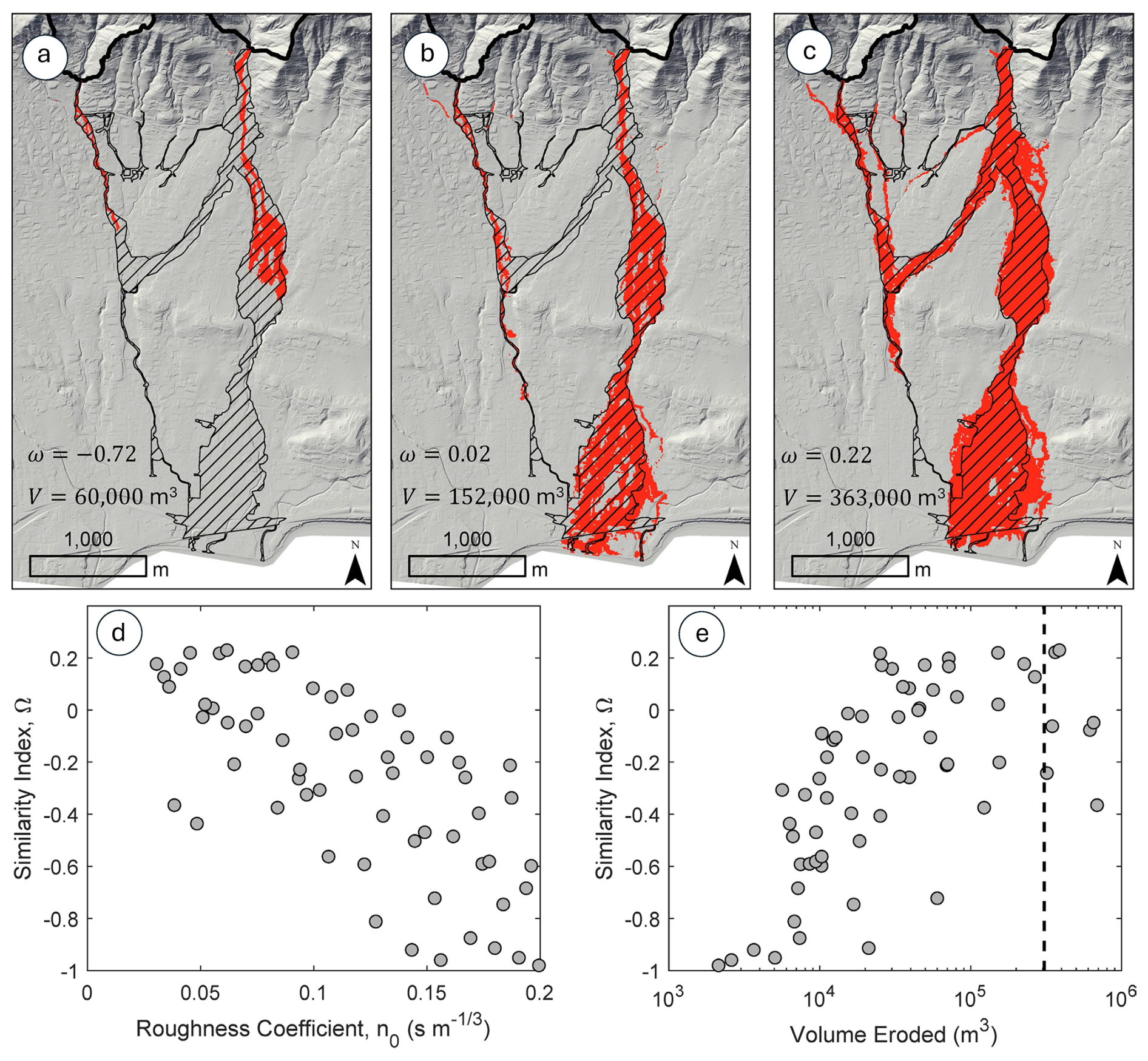
Figure 2 Comparisons between modeled and observed area inundated for flows where the volume of sediment eroded from the upper watersheds was approximately (a) 60 000 m³ (parameters: k_s=11.2, r_max=1.3, η₀=0.15, F=0.04, δ=0.09, RI_fac=0.53) (b) 152 000 m³ (parameters: k_s=11.1, r_max=0.87, η₀=0.05, F=0.03, δ=0.1, RI_fac=0.6) (c) and 363 000 m³ (parameters: k_s=10.7, r_max=1.0, η₀=0.091, F=0.03, δ=0.07, RI_fac=1.28). The observed volume of sediment eroded from the upper watersheds was 307 000 m³. (d) The similarity index, ω, is greatest when the hydraulic roughness coefficient is low. This indicates a better fit between modeled and observed inundation extents when using lower roughness coefficients, especially values less than 0.1 (e) The similarity index generally increases with the volume of sediment eroded from the upper watersheds. Model performance, as quantified by the similarity index, is best when the modeled volume eroded is close to matching the observed volume eroded (dashed black line).

4 Results

4.1 Observed and Modeled Area Inundated

The modeled area inundated, defined as the area below the watershed outlets where flow depth exceeded 0.1 m matches the observed area inundated well within a portion of the explored parameter space. The similarity index is generally greater when the hydraulic roughness coefficient, n₀ is less than 0.1 (Fig. 2). The amount of sediment eroded from the upper watersheds varies substantially from roughly 2000 m³ to nearly 700 000 m³ (Figs. S3, 2). The observed eroded volume of 307 000 m³ falls near the upper range of most simulated erosion volumes (Fig. 2). The similarity index generally increases with erosion volume and approaches its maximum value of roughly 0.23 where the simulated and observed erosion volumes are similar (Fig. 2).

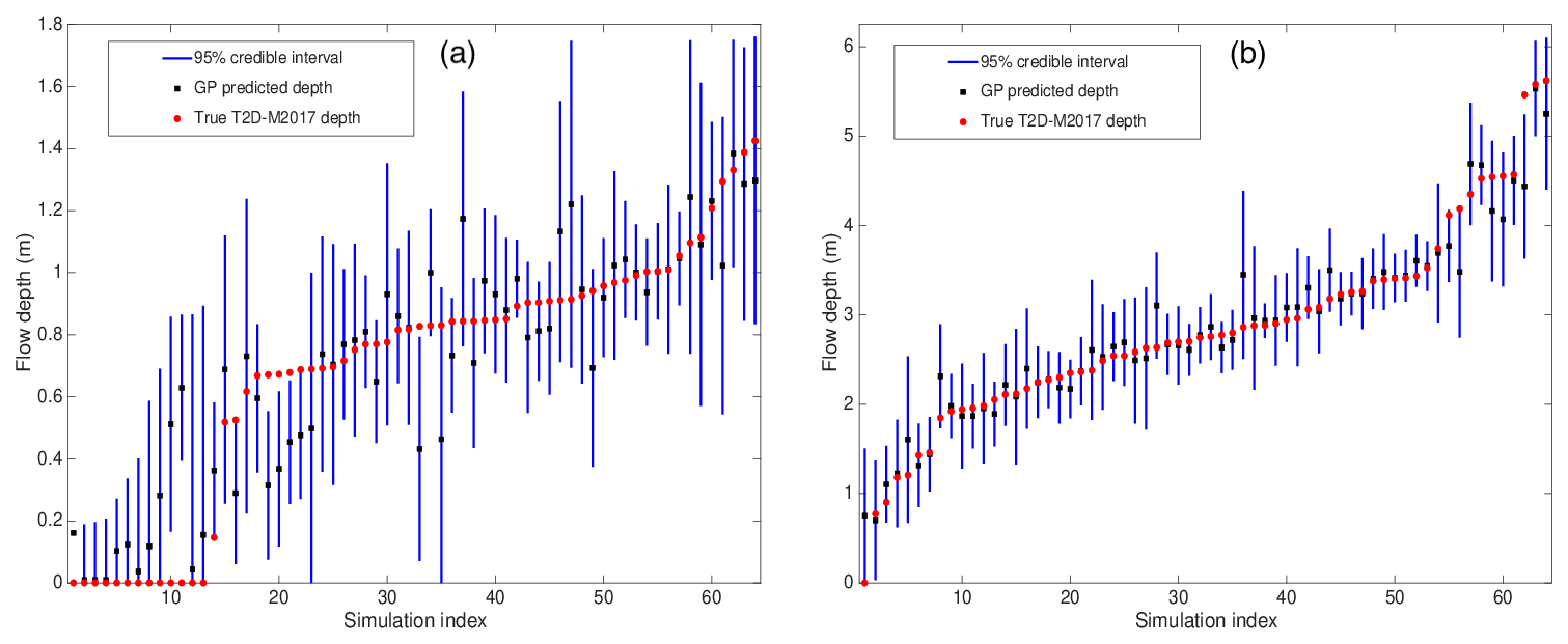
Figure 3 Leave-one-out experiments for (a) a location on the fan and (b) a location in the channel (see Fig. 7 for details). In each panel, indices were sorted based on the T2D-M2017-simulated peak flow depth (red dots). GP predictive means for these left-out scenarios were plotted as black squares while the 95 % credible intervals were plotted as vertical blue bars.

4.2 Emulator performance

A good test of an emulator's performance is its ability predict left-out values using the rest of the design simulations, and so we examined leave-one-out predictions for our debris flow simulations. A GP emulator was re-fit 64 times, each with a set of N=63 design simulations and one left-out simulation; each GP was then used to predict its left-out simulation values. The range parameter estimates across these 64 emulators were very stable. More specifically, we found the coefficients of variation for each of the six range parameter values to be between 0.03–0.15 indicating that the relative influence of any input to the GP was not swayed strongly by any single flow simulation. For illustrative purposes, we focused on two points of interest – one located in a channel and one on the adjacent fan surface where flow is relatively unconfined. Note, the training simulations were designed to generate a large range of flow depth values. In Fig. 3, for both cases, we sorted the simulations by their left-out flow depths, y, and predicted each with a credible interval centered at the mean of the GP prediction, $\stackrel{\mathrm{̃}}{y}$. We found root mean squared errors from these leave-one-out experiments of 0.16 and 0.36 m for the locations on the fan and in the channel, respectively. Further, we observed that 89 % (fan location) and 94 % (channel location) of the simulated depths fall within their predictive credible intervals. These numbers are slightly below the anticipated 95 % coverage, but this is likely due to the relatively small training set. The rule-of-thumb for the size of a GP training set is at least 10× the number of input parameters varied (Berger and Smith, 2019). In the case of the fan location, roughly one third of the simulations resulted in no inundation. While this behavior was anticipated – some training scenarios do not lead to debris flow inundation on the fan – it also effectively reduced the size of the training set for the GP to learn how inundation depths change as scenarios change. Cases where a large fraction of training runs that result in zero (no inundation) outputs are challenging for GP emulation. Although Spiller et al. (2023) introduced methodology to address this challenge in the scalar-output case, applying this methodology to the PPE is an on-going area of research.

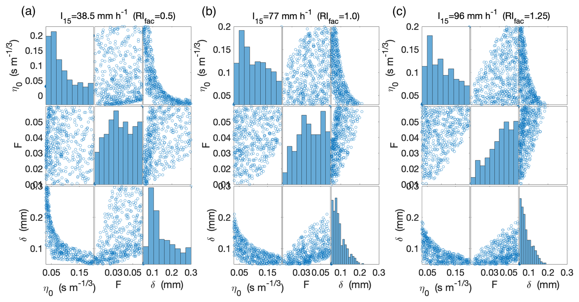
Figure 4 (a) $I_{\mathrm{15}}=\mathrm{38.5}\mathrm{mm}{\mathrm{h}}^{-\mathrm{1}}$ (RI_fac=0.5); (b) $I_{\mathrm{15}}=\mathrm{77}\mathrm{mm}{\mathrm{h}}^{-\mathrm{1}}$ (RI_fac=1); (c) $I_{\mathrm{15}}=\mathrm{96}\mathrm{mm}{\mathrm{h}}^{-\mathrm{1}}$ (RI_fac=1.25). Each panel contains histograms and pairwise scatter plots of η₀, F, and δ that result in GP volume predictions ± 10 % of the targeted volumes. The target volume for a given I₁₅ is defined as that predicted by the Gartner et al. (2014) Emergency Assessment Volume model (Gartner et al., 2014). Note that the vertical and horizontal labels apply to each scatter plot in the matrix, but only the horizontal labels apply to the histograms.

4.3 Sensitivity analysis

A crucial step to fitting a GP is estimating the range parameters. Smaller range parameters indicate that the corresponding model parameter has more influence on the debris flow model output of interest (i.e. maximum flow depth). (See the leftmost column of Table 1). Modeled peak flow depth was most sensitive to the hydraulic roughness coefficient, followed by effective grain size, rainfall intensity, fraction of stream power effective in sediment detachment, and saturated hydraulic conductivity; it was relatively insensitive to the maximum soil thickness.

4.4 Effects of rainfall intensity on runout

One will often want to use GP surrogates in a predictive mode. We used surrogates to predict how the probability of debris flow inundation varies across three different rainfall scenarios as defined by rainstorms with a peak I₁₅ of 38.5 mm h⁻¹ (RI_fac=0.5), 77 mm h⁻¹ (RI_fac=1), and 96 mm h⁻¹ (RI_fac=1.25), respectively. Figure 4 shows scatter plots from (500 volume-targeted) samples of effective grain size (δ), effective sediment detachment fraction (F), and hydraulic roughness (η₀) against each other along with histograms of samples in each parameter. As I₁₅ increases, F goes from nearly uniform to skewed toward higher values while δ values cover the whole range of grain sizes for lower I₁₅, but skew toward the smallest grain sizes for high values of I₁₅. Greater values of I₁₅ are associated with greater target debris flow volumes. The observed shifts in the relevant portion of the parameter space reflect this change. For example, greater values of F and smaller values of δ produce larger debris flows (Fig. S3).

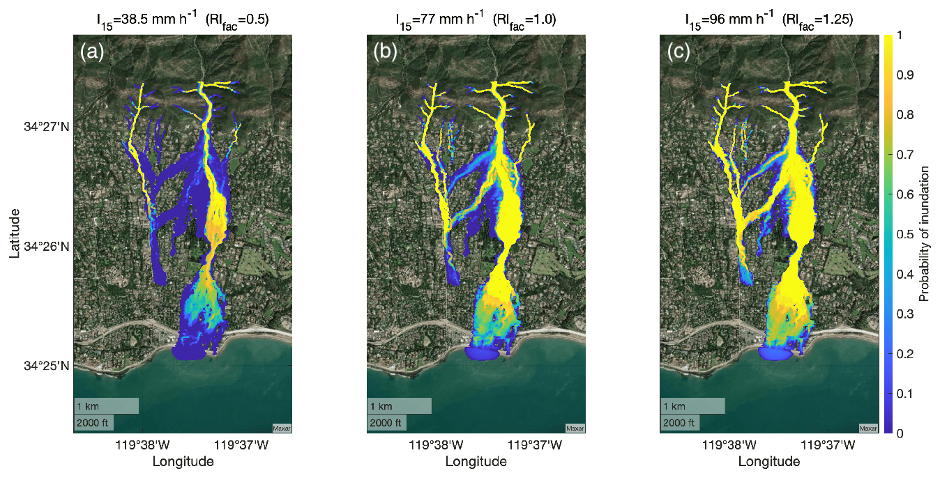
Figure 5 Probability of inundation for three rainfall scenarios associated with immediate postfire conditions: (a) $I_{\mathrm{15}}=\mathrm{38.5}\mathrm{mm}{\mathrm{h}}^{-\mathrm{1}}$ (RI_fac=0.5); (b) $I_{\mathrm{15}}=\mathrm{77}\mathrm{mm}{\mathrm{h}}^{-\mathrm{1}}$ (RI_fac=1); (c) $I_{\mathrm{15}}=\mathrm{96}\mathrm{mm}{\mathrm{h}}^{-\mathrm{1}}$ (RI_fac=1.25).

Figure 5 shows a map of the probability of inundation for each rainfall scenario. The spatial footprint of area with a high probability of inundation increases substantially as I₁₅ increases from 38.5 to 77 mm h⁻¹. Such a probabilistic analysis using only T2D-M2017 simulations would be computationally taxing.

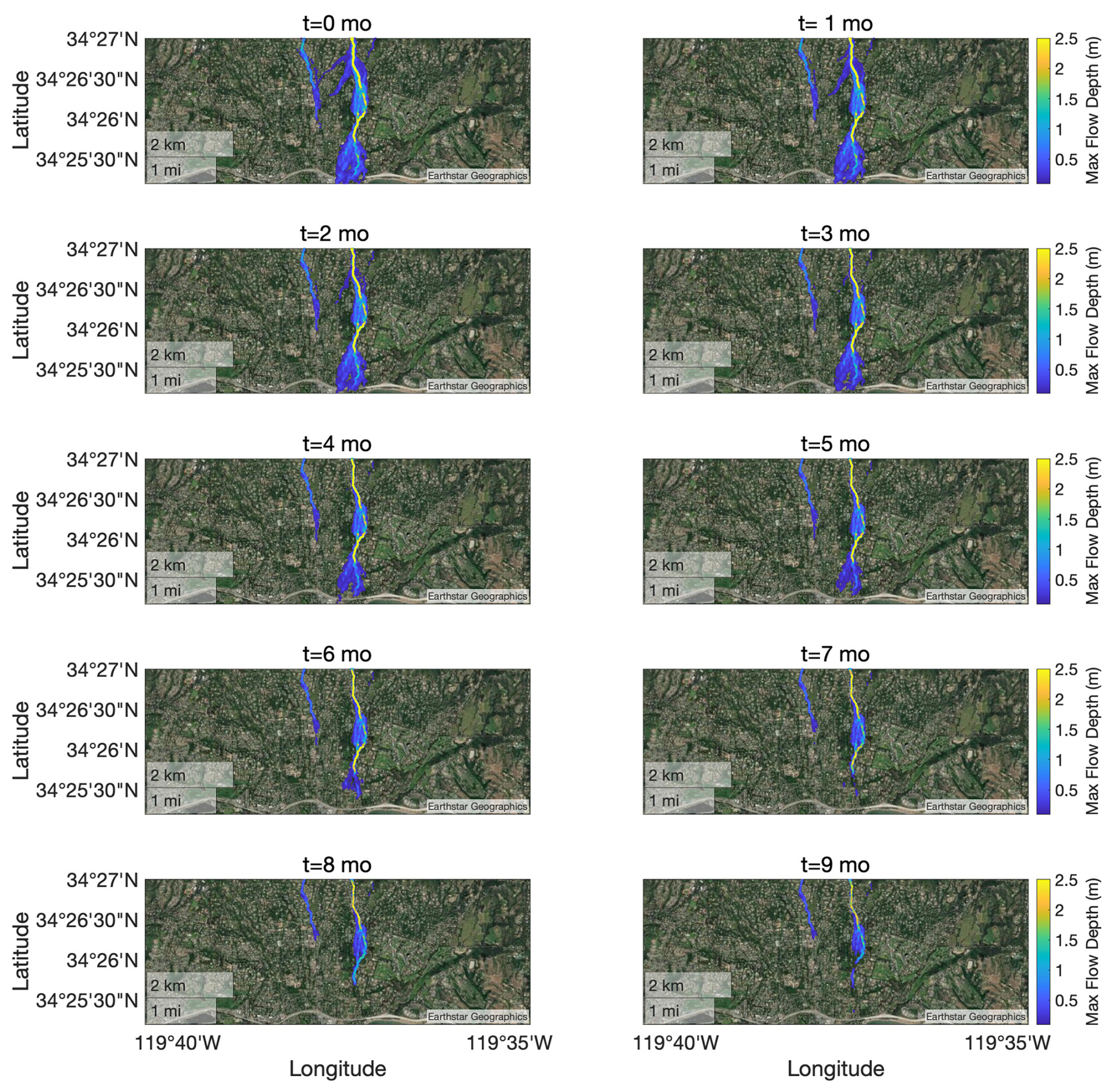
Figure 6 Maximum flow depth for different times since fire. Values of the hydraulic roughness coefficient and saturated hydraulic conductivity vary with time based on data from Liu et al. (2021) (Fig. S2). Saturated hydraulic conductivity is approximately 5 mm h⁻¹ immediately after fire and increases to almost 15 mm h⁻¹ after one year. The hydraulic roughness coefficient increases from roughly 0.05 immediately after fire to 0.2 after one year. All of the other parameters are set to the center value of their range. For contrast, the maximum color bar limit is set to 2.5 m although in the channels towards the north, maximum flow depth exceeds 2.5 m.

4.5 Effects of postfire recovery on runout

Liu et al. (2021) developed parametric best-fit curves to model the change in saturated hydraulic conductivity and hydraulic roughness as a function of time following fire in the nearby San Gabriel Mountains. Using these relationships, and setting other parameters to the center of their respective ranges, we used the GP emulator to explore the effects of temporal changes in the hydraulic roughness coefficient and saturated hydraulic conductivity. Both peak flow depth and area inundated in response to the observed rainstorm would decrease substantially over the first six months following fire (Fig. 6). For example, US Highway 101, which runs perpendicular to the direction of flow near the distal portion of the fan, would only be inundated when the rainstorm occurs within the first 3 months following fire. If the observed rainstorm were to have occurred 12 months following the fire, the simulated inundation area would be limited to channels near the fan apex.

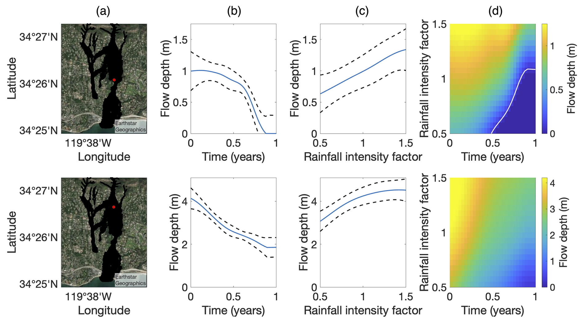
Figure 7 Exploration at one location on the fan (top row) and one location in the channel (bottom row). Panels in column (a) indicate locations of all emulated flow depths (black) and those being explored in detail (red). Panels in column (b) show peak flow depth as a function of time since fire (solid blue curve) along with 95 % credile interval bounds (dashed black curves). The hydraulic roughness coefficient and saturated hydraulic conductivity are parameterized as a function of time since fire (Liu et al., 2021) while RI_fac=1 and all other parameters set at their central values. (Note that the vertical scales are different; the maximum flow depth on the fan is roughly 1 m, and that in the channel is roughly 4 m.) Panels in column (c) show peak flow depth versus rainfall intensity with the hydraulic roughness coefficient and saturated hydraulic conductivity set to their respectively minimum values, which could be interpreted as a worst-case scenario immediately after a fire, and all other parameters set at their central values. Panels in column (d) contain color maps for maximum flow depth at these two locations varying all combinations of rainfall intensity and time since fire, which determines the hydraulic roughness coefficient and saturated hydraulic conductivity (Liu et al., 2021). The white contours indicate the values of time since fire and rainfall intensity leading to a peak flow depth of 10 cm or more at the selected points.

We can also explore the effects of rainfall intensity and temporal changes in hydraulic roughness and saturated hydraulic conductivity following fire by examining flow depth at distinct points of interest. Again, we considered the same two points for illustrative purposes, one located in a channel and one on the adjacent fan surface where flow is relatively unconfined (Fig. 7). For a given time since fire, peak flow depths are greater in the channel relative to the fan surface, as expected. Peak flow depth decreases gradually over the first several months at the point on the fan before dropping substantially after approximately nine months. Peak flow depths decrease over the first year following fire in the channel location from roughly 4 to 2 m. Visualizing peak flow depths as a function of time since fire and rainfall intensity can be helpful for assessing temporal shifts in the magnitude of rainfall associated with potential debris-flow impacts at different locations. For example, the area inundated by a flow in response to a rainstorm characterized by RI_fac=1 would decrease substantially over the first 9 postfire months (Fig. 6).

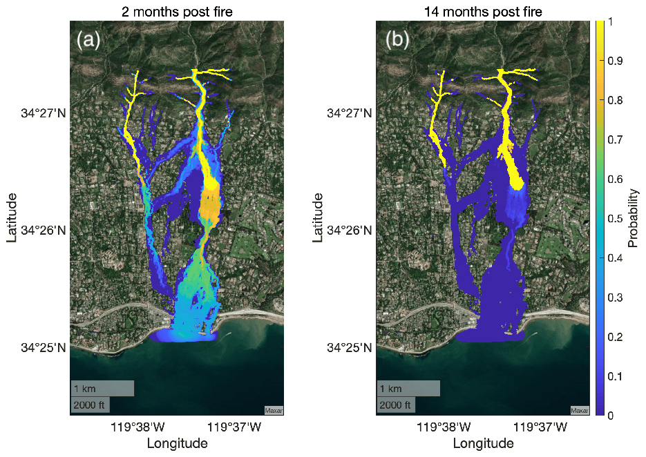
Figure 8 Probability of inundation maps, where a location is considered inundated if the maximum flow depth exceeds 10 cm. To calculate this probability, all parameters except the Manning coefficient and saturated hydraulic conductivity are set to their central values with the latter set to values corresponding to (a) the 2 month and (b) 14 month estimates from Liu et al. (2021), respectively.

We further used the emulator to produce probabilistic maps of inundation at different times following fire (Fig. 8). Differences in the spatial patterns of inundation likelihood are apparent between scenarios where the storm occurs 2 months following the fire versus 14 months. We identified a location as being inundated if peak flow depth exceeds 0.1 m. RI_fac was set to 1. All parameters were set to their central values except for saturated hydraulic conductivity and the hydraulic roughness coefficient. The latter parameter was sampled from the distribution suggested by Liu et al. (2021) while the former was set to the 2 and 14 month values, respectively, estimated from the same study. The probability MC calculation was carried out with 100 samples.

5 Discussion

5.1 Model Performance

T2D-M2017 was able to provide reasonable estimates of inundation extent. Across the 64 T2D-M2017 simulations, which only sparsely cover the parameter space, the maximum similarity index of 0.23 is similar to what other debris flow runout models have achieved when calibrated to the study area. For example, a runout model based on an empirical flow routing algorithm achieved a similarity index of 0.25 when applied to the San Ysidro watershed (Gorr et al., 2022) and physics-based models (i.e. RAMMS, FLO-2D, D-CLAW) with various rheological assumptions had similarity indices between 0.23 and 0.26 (Barnhart et al., 2021). Here, the similarity index was generally greater when the volume of sediment eroded from the upper watersheds was closer to the observed volume eroded. This observation is consistent with flow volume being an influential factor in debris flow runout, including specifically in our study area (Barnhart et al., 2021).

Although the T2D-M2017 model was able to reproduce both the observed sediment volume eroded from the upper watershed and the inundation pattern on the fan, the resulting spatial patterns of erosion are not consistent with observations of widespread incision in higher order channels (Morell et al., 2021; Dunne et al., 2025) (Fig. S4). Modeled erosion patterns are characterized by incision on hillslopes in areas of concentrated flow and in low order channels, which was also observed after the debris flow event (Alessio et al., 2021). We attribute the limited amount of modeled erosion in high order channels, in part, to model assumptions and limitations. For example, since there is no established and generally applicable methodology for quantifying sediment entrainment rates by debris flow, the model neglects sediment entrainment when the volumetric sediment concentration exceeds 0.4 (McGuire et al., 2016, 2017). As a result, intense erosion that leads to high sediment concentrations and debris flow initiation in low order channels could result in higher order channels acting as transport zones for the debris flows that developed at lower drainage areas. We accepted this limitation since our main objective was to simulate the downstream effects of debris flows rather than their growth rates or erosion patterns. Improved representation of sediment entrainment processes, particularly in channels and in portions of flow with sediment concentrations approaching those associated with debris flows, would be beneficial for future applications.

5.2 Model Sensitivity

Fire effects on soil and vegetation properties that affect the initiation and growth of runoff-generated debris flows are most extreme in the first few months following fire (DeGraff et al., 2015; Thomas et al., 2021). Potentially rapid changes in hydrologic conditions following fire limit the time window for gathering data needed to constrain parameters for postfire runoff and erosion models, including the model used here. Aside from rainfall intensity, which will not be affected by the fire, we found that hydraulic roughness, the representative grain size, the fraction of stream power effective in sediment entrainment, and saturated hydraulic conductivity played the most important roles in controlling peak debris flow depth. Additional model testing across fire-prone regions in different geologic and climate settings is needed to assess model performance and determine the extent to which results related to parameter sensitivity are generalizable. Soil thickness, which provides a limit on the maximum depth of incision, could be more influential if the model better reproduced observed erosion depths throughout the channel network. In simulations, debris flow sediment was primarily sourced from more widespread shallow incision on hillslopes and low-order channels. Therefore, there were relatively few locations in the landscape where the maximum depth of incision was achieved. Nonetheless, these results provide observational targets that can help focus future efforts to collect perishable postfire data.

Peak flow depth was most sensitive to hydraulic roughness. We hypothesize that hydraulic roughness plays an important role in controlling inundated area and peak flow depths because of its influence on both modeled sediment detachment rates and flow resistance. Lower values of hydraulic roughness are associated with increased erosion from the upper watersheds (Fig. S3). Saturated hydraulic conductivity will influence the rate at which sediment is detached by overland flow since it plays a role in controlling runoff magnitude and stream power. Increased rates of sediment detachment lead to increases in flow volume, which in turn act to increase runout and inundation potential (Barnhart et al., 2021). Grain size,which is the second most influential parameter, similarly influences flow volume since a larger grain size will encourage more rapid deposition of sediment. The volume of sediment eroded from the upper watersheds decreases with increasing δ (Fig. S3).

Our evaluation of parameter sensitivity indicates that constraints on postfire values for hydraulic roughness, saturated hydraulic conductivity, fraction of stream power effective in sediment entrainment, and the grain size distribution of sediment entrained in debris flows would be beneficial for improving estimates of debris flow runout estimates. Burn severity is likely to play a substantial role in a fire's initial effect on these variables (Moody et al., 2016; McGuire and Youberg, 2020). In addition, attempts to capture changes in debris flow runout as a function of time since fire would benefit from methods to parameterize temporal changes in these influential parameters. Fire-driven reductions in hydraulic roughness are commonly cited as a cause for increased runoff and erosion (McGuire and Youberg, 2020; Stoof et al., 2015) as are increases in soil erodibility, which could be reflected in greater values of F. There are few constraints on the temporal changes in hydraulic roughness or F following fire, which may be facilitated by changes in vegetation cover, ground cover, and/or grain roughness. In addition to being parameterized based solely on time since fire, changes in hydrologic model parameters, such as hydraulic roughness or saturated hydraulic conductivity, could be tied to changes in remotely sensed vegetation indices (Thomas et al., 2021).

Particularly in southern California (Doehring, 1968; Florsheim et al., 1991; DiBiase and Lamb, 2020) and other tectonically active regions in the western USA (Roering and Gerber, 2005), fire can promote substantial increases in dry ravel activity on hillslopes that can reduce hydraulic roughness by increasing the availability of fine sediment in channels. Hydraulic roughness may then increase over time as dry ravel deposits are progressively eroded during postfire rainstorms (Tang et al., 2019). Temporal changes in debris flow sediment source locations (Guilinger et al., 2020) and coarsening of particle size distributions due to preferential erosion of fines would also influence the effective grain size in the model. In practice, it is not clear how to quantitatively connect this single grain size parameter to the particle size distribution of hillslope or channel sediment, especially when flows contain boulders. Postfire changes in saturated hydraulic conductivity can be inferred from calibration of hydrologic models (Liu et al., 2021), rainfall simulator experiments at the small plot scale (Robichaud et al., 2016), and point scale measurements (Ebel, 2020; Ebel et al., 2022; Perkins et al., 2022). While some general patterns have been observed between time since fire and values of saturated hydraulic conductivity, there is substantial site-to-site variability (Ebel and Martin, 2017). The level of uncertainty in influential model input parameters and how they change over time highlights the need for probabilistic assessments of debris flow runout, which emulators can help to achieve by facilitating rapid exploration of large parameter spaces.

5.3 Debris flow hazards

Rainfall is a necessary driver for debris-flow initiation and the model was also sensitive to rainfall intensity, specifically a rainfall intensity factor which we used to scale an observed rainfall intensity time series. This finding is consistent with observations that postfire basin-scale sediment yields (Pak and Lee, 2008) and debris flow volume (Gartner et al., 2014; Gorr et al., 2024) increase with rainfall intensity averaged over durations of 60 min or less. Short duration (sub-hourly) bursts of high intensity rainfall are effective at generating infiltration-excess overland flow that can trigger debris flows in recently burned steeplands (Kean et al., 2011; Nyman et al., 2011; Esposito et al., 2023). Since the spatial and temporal distributions of rainfall can influence flood and debris-flow processes (Oh et al., 2024; McGuire et al., 2021; Zhou et al., 2021), future work could consider sensitivity of debris-flow runout to storm characteristics beyond peak intensity.

Emulators can be useful for generating probabilistic maps of debris flow inundation in response to design storms with different rainfall intensities or examining changes at particular points of interest. In cases where there are specific values at risk downstream of a burned area, rapid exploration of debris flow characteristics (i.e. peak flow depth) as a function of rainfall intensity could help define impact-based rainfall thresholds that could be used for planning and warning purposes. In other words, one could take advantage of the emulator's computational efficiency to determine not only the rainfall intensity required to initiate a debris flow, but also the rainfall intensity required to produce a debris flow that would impact a prescribed area of interest with some prescribed depth of flow. Such estimates could be particularly useful for assessing building damage (Barnhart et al., 2024).

The computational cost of many physically-based debris flow models is a limitation in applications that are time sensitive, such as rapid postfire hazard assessments. Postfire debris flows in the western USA, such as those that occurred near Montecito, may occur before the fire has been officially contained and within weeks or months of fire ignition. Approximately 23 % of postfire debris flow events, for example, initiate in the first 60 d following fire (McGuire et al., 2024). The emulator methodology presented here provides one avenue for minimizing computation times, since an initial suite of simulations can be used to train the emulator which can later be applied with substantially less computational effort to generate a probabilistic hazard map for a specific scenario. Further, as emulators do not depend on a prior distribution characterizing scenario randomness, modeling scenario randomness can be done in parallel or after emulator construction. Likewise, an emulator could even be trained prior to a fire. Analogous approaches have been employed in related applications (Rutarindwa et al., 2019; Spiller et al., 2020). Within the context of postfire hazards, an emulator could be used to assess debris-flow runout and inundation downstream of a burned area in response to a design or forecast rainstorm. Atmospheric model ensembles, for example, can provide estimates of peak 15 min rainfall intensity over watersheds of interest that could be used to constrain a distribution of rainfall intensity factors (Oakley et al., 2023).

We focused on applications of surrogate modeling for postfire runoff-generated debris flows since accelerating MC calculations could be particularly beneficial within the context of rapid hazard assessments after fire when there are time constraints. However, the methodology presented here could similarly be applied to debris flows in unburned settings as well as to a broader range of geophysical flows. Runoff-generated debris flows, for example, can initiate in unburned alpine environments through processes that are similar to those that operate in recently burned watersheds (Coe et al., 2008; Tang et al., 2020; Gregoretti and Fontana, 2008; Bennett et al., 2014). There remain additional challenges to constructing robust and efficient emulators of geohpysical mass flow models that warrant future study: handling large numbers of zero-output pixels; and developing efficient adaptive design strategies that can reliably capture simulator behavior at every pixel of interest.

6 Conclusions

We applied a computationally expensive physics-based morphodynamic model and cost effective surrogates based on Gaussian process models to simulate postfire debris flows. We employ a Gaussian Process surrogate model, or emulator, to approximate peak flow depth from a physics-based morphodynamic model, T2D-M2017. The emulator is able to approximate the peak flow depth with a mean squared error that is generally in the range of 0.1–0.2 m when using a modest training data set built from 64 T2D-M2017 simulations. By parameterizing postfire changes in hydraulic roughness and saturated hydraulic conductivity, we demonstrated that the area inundated by postfire flows decreases substantially over a time period as short as 9 months. In many instances, the temporal persistence of debris flow hazards after fire is assessed through changes in the rainfall intensity required to intiate debris flows. Here we illustrated the utility of cost-effective surrogates for extending this type of analysis to include information about how flow runout changes with time since fire. The range parameters associated with the emulator provide a metric for the relative importance of input parameters, which provides guidance for those that are most important to constrain for forward modeling of debris flow runout. We found that peak flow depths are most sensitive to changes in hydraulic roughness and grain size, while slightly less sensitive to a parameter related to sediment entrainment, a rainfall intensity factor, and saturated hydraulic conductivity. We highlighted the emulator's ability to provide rapid estimates of peak flow depth for parameter combinations that were not part of the training data set by generating probabilistic maps of inundation as a function of time since fire. Emulator-based analyses can also facilitate rapid Monte Carlo calculations of inundation probability, making them a promising option for rapid postfire hazard assessments and scenario planning before a fire starts.