Identification of hydro-meteorological drivers for forest low greenness events in Europe

Extreme hydro-meteorological events can have a substantial impact on vegetation and ecosystems. In particular, with heatwaves and droughts projected to become more frequent due to climate change, understanding their effects on forests is crucial. In this study, we present a novel, large-scale, spatially explicit analysis of forest browning drivers across Europe, using a homogeneous and automated random forest modeling framework. By running independent models at each 0.5° grid point, we enable a region-specific comparison of hydro-meteorological drivers, capturing the diversity of forest responses across the continent. We identify the most relevant hydro-meteorological predictors of low normalized difference vegetation index (NDVI) events at monthly to annual timescales, using NDVI data from the Advanced Very High Resolution Radiometers (AVHRR) and climate variables from ERA5 and ERA5-Land reanalyses. These predictors include maximum temperature at 2 m precipitation, surface latent heat flux, and soil moisture up to 18 months before the observed browning. The random forest model exhibits a high prediction skill over most grid points in Europe, with a critical success index greater than 0.75 for 65 % of grid points. Notably, warm and dry conditions in spring and early summer emerge as essential predictors. We also uncover multi-year influences, with soil moisture and temperature anomalies from the preceding year playing a significant role, especially in Scandinavia and for coniferous forests. The random forest approach further reveals non-linear relationships, such as both positive and negative precipitation anomalies at different lags contributing to browning risk.

1 Introduction

Forests cover about 202 million ha in Europe (FAO, 2020), or about 32 % of its land area. Forests offer essential ecosystem services such as soil conservation and fertility (Jenkins and Schaap, 2018), water regulation and purification (EFI, 2025; Postel and Thompson, 2005; Thompson et al., 2011; Neary et al., 2009), protection against landslides and avalanches, air cleaning, wood production, habitat for specialized biodiversity (Brockerhoff et al., 2017), without forgetting their aesthetic, spiritual, and recreational value (Neary et al., 2009; Brockerhoff et al., 2017). These essential ecosystem services are at risk due to climate change, which causes increased occurrences of detrimental conditions for forests, such as insect outbreaks (Pureswaran et al., 2018) and increased drought frequency (Adams et al., 2017; Senf et al., 2020; Masson-Delmotte et al., 2021).

The health of trees and forests strongly depends on hydro-meteorological conditions. In particular, anomalously dry and hot conditions, especially if they occur over an extended period, can be highly detrimental to forests (Leuzinger et al., 2005; Senf et al., 2020; Brodribb et al., 2020). Droughts can lead to early leaf senescence, parasite infestations, higher fire risk, loss of canopy greenness, and enhanced crown and tree mortality (Brun et al., 2020; Frei et al., 2022; Mariën et al., 2021; Sperlich et al., 2015). Adverse air and soil humidity conditions can also impact tree health, such as anomalies in vapor-pressure deficit (Grossiord et al., 2020; McDowell et al., 2022), potential evapotranspiration (Young et al., 2017), or soil moisture (Alavi, 2002). Large and persistent deviations from normal conditions can impact the photosynthetic capacity and carbon intake (Hinckley et al., 1979; Sperlich et al., 2015). In addition, consecutive dry years can increase tree vulnerability and lead to a larger impact on forests than the combined effect of individual non-consecutive dry years (Anderegg et al., 2015). Adverse hot and dry conditions causing forest browning are expected to become more frequent and more intense under climate change (IPCC, 2022). Moreover, longer growing seasons can amplify drought effects due to earlier spring leaf unfolding, as shown by Meier et al. (2021) for Swiss broadleaved forests.

Forest canopy greenness, widely employed as a proxy for vegetation conditions, exhibits strong sensitivity to hydro-climatic variability across sub-seasonal to interannual timescales (Obuchowicz et al., 2023). Satellite-based remote sensing, particularly vegetation indices such as the Normalized Difference Vegetation Index (NDVI), enables a systematic and spatially consistent monitoring of canopy greenness across large regions, offering the capability for the detection and attribution of forest stress (Liu et al., 2013; Sun et al., 2021). For example, satellite-derived low NDVI values have been associated with severe canopy impacts during the 2013 and 2018 droughts in Germany (Brun et al., 2020; Buras et al., 2020; West et al., 2022). Hermann et al. (2023) introduced a pragmatic and systematic approach that advances this capability by explicitly linking NASA Terra MODIS observations to multi-annual meteorological records. Their methodology identifies low-NDVI events at a 50 km spatial scale across Europe, showing that reduced summer forest greenness is consistently preceded by anomalous temperature and precipitation patterns during the preceding months and seasons. Satellite imagery is a powerful tool for monitoring drought impacts, yet the wide range of available sensors, each with distinct characteristics, requires careful consideration when selecting the most suitable ones (Verbesselt et al., 2010; West et al., 2019). Among these, the Advanced Very High Resolution Radiometer (AVHRR) is unique in providing a continuous 40 year record (Weber et al., 2021; Dupuis et al., 2024; Barben et al., 2024). AVHRR is onboard the National Oceanic and Atmospheric Administration (NOAA) and the European Organisation for the Exploitation of Meteorological Satellites (EUMETSAT). AVHRR provides global coverage in the Global Area Coverage format with a spatial resolution of approximately 0.083°, and higher-resolution data in the Local Area Coverage (LAC) format at about 0.01°.

An improved understanding of the hydro-meteorological drivers of decreased canopy greenness, and of their relative contributions across temporal scales, will benefit the predictive capacity in forest health assessments. In turn, successful predictions of forest health would benefit the design and implementation of efficient protection measures. Such predictions are expected to be possible due to a range of drivers affecting the greenness of trees and acting on timescales of weeks to years. For example, precipitation and temperature conditions strongly influence forest health. Hermann et al. (2023) showed that, in Europe, reduced summer forest greenness is preceded by positive temperature anomalies and negative precipitation anomalies in spring. Preventive action can be taken before such conditions trigger forest vulnerability. Examples include forest fire prevention (Ferreira et al., 2015), sanitation logging, and predation using long-legged flies (Medetera spp.) to prevent spruce bark beetle (Ips typographus) infestations (Weslien et al., 2024). On longer timescales of years to decades, a good understanding of forest susceptibility to meteorological conditions can help managers prioritize regions for adaptation and select tree species that are better suited to future climate conditions. In this context, we choose to study hydro-meteorological variables available from operational forecasts covering the subseasonal-to-seasonal (S2S) timescale. For example, the European Centre for Medium-Range Weather Forecasts (ECMWF) sub-seasonal forecasts cover timescales up to 1.5 months in advance and have been used to predict extreme events (Domeisen et al., 2022) and their surface impacts (White et al., 2022) from a range of atmospheric conditions. In particular, the ECMWF S2S forecast model includes the following hydro-meteorological variables: 2 m temperature, precipitation, soil moisture with soil-water equivalent, and surface latent heat flux (as an estimate of potential evapotranspiration). Our analysis establishes a link between these hydro-meteorological variables and forest health, allowing forest practitioners to anticipate adverse conditions based on S2S forecasts. In addition, machine learning can leverage extensive data to predict vegetation states based on weather and climate conditions (Nay et al., 2018; Kladny et al., 2024). For instance, Lasso regression can identify key drivers through feature selection and performs well in the presence of correlated variables (Tibshirani, 1996; Vogel et al., 2021). Random Forest, a more flexible model based on decision trees, is an interpretable method that ranks predictor importance and captures non-linear relationships (Breiman, 2001; Oliveira et al., 2012).

In this work, we introduce a novel, automated framework to identify and quantify adverse monthly to annual hydro-meteorological conditions driving forest browning across Europe. We employ a random forest (RF) classification model to predict summer low greenness events (July–August), using NDVI anomalies as a proxy for forest health. The RF model offers both flexibility and interpretability, making it well-suited for capturing complex, non-linear relationships between climate variables and vegetation response. We run independent RF models at each 0.5° grid point, enabling a region-specific identification of key predictors and time windows. This approach allows us to capture the diversity of forest-climate interactions across Europe, rather than relying on a one-size-fits-all model. Our goal is to pinpoint the most critical hydro-meteorological drivers at monthly to annual timescales, using only variables that are available from operational S2S forecast systems. By linking forest browning to predictable climate conditions, our method aims to provide actionable insights for forest managers, offering valuable lead time to anticipate and mitigate the impacts of climate extremes through targeted interventions.

2 Data

2.1 NDVI data

Forest browning can be assessed using a range of indices, including vegetation indices based on satellite observations, for a direct assessment of vegetation stress over large areas (Bannari et al., 1995; Zeng et al., 2022). We here employ the normalized difference vegetation index (NDVI, Kriegler et al., 1969; Rouse et al., 1974), a measure of vegetation greenness widely used to monitor the health of forests (Zhou et al., 2003; Pettorelli et al., 2005; Buras et al., 2021; Rumpf et al., 2022). When measured over large areas, the NDVI captures forest vitality losses resulting from reduced canopy greenness or tree mortality (West et al., 2019; Nash et al., 2017; Wang et al., 2020; Yan et al., 2025).

The NDVI is defined by $\text{NDVI}=\frac{\text{NIR}-\text{red}}{\text{NIR}+\text{red}}$, where NIR and red represent the spectral reflectance measurements in the near-infrared (NIR) and red portions of the electromagnetic spectrum, respectively. The NDVI values corresponding to vegetation typically lie between 0 and 1, with values close to one indicating very green, dense, and healthy vegetation. Lower NDVI values indicate either sparse vegetation or browning of the vegetation, a visible sign that the plants are undergoing stress or damage.

We use the NDVI 10 d composite dataset generated from the AVHRR LAC data (Dupuis et al., 2024; Barben et al., 2024; Weber et al., 2021). This dataset is archived at the University of Bern, Switzerland, and contains data from the AVHRR sensors from the NOAA and Metop satellite series (MetOp1, MetOp2, and MetOp3). The NDVI compositing is generated by retaining the 10 d median value of NDVI (Asam et al., 2023). Prior to that, the dataset was orthorectified, radiometrically calibrated, and filtered for clouds, and the NDVI values were spectrally corrected for the different versions of the AVHRR instrument (see Appendix A for further details). The advantage of using the AVHRR dataset over Europe is the long period of data availability, from 1981 to 2022, and the good trade-off between temporal resolution (10 d) and spatial resolution (0.01° N × 0.01° W, corresponding to an effective footprint of approximately 1 km²). We discarded NOAA-15 due to poor data quality and MetOp3 due to the absence of specific correction coefficients for the spectral response function (see Fig. A1 in Appendix A for the time distribution of the satellites used). As several platforms (NOAA-6 to -18 and the MetOp-series) may be available for a given 10 d composite, we selected the maximum NDVI value among the MED (10 d median value composite) NDVI values to obtain a single time series. Selecting the maximum among the MED diminishes the impact of potential disturbances such as clouds, snow, and aerosols, which tend to lower NDVI values (Holben, 1986; Cihlar et al., 1994).

AVHRR LAC data has a medium spatial resolution (1.1 km at nadir) and may not capture fine-scale variability in vegetation greenness. Higher resolution datasets, such as NDVI data derived from Sentinel-2, can better capture high-resolution vegetation dynamics (Benson et al., 2024; Kladny et al., 2024), but offer a lower temporal resolution. To identify low-greenness events, we followed the method of Hermann et al. (2023) (see Sect. 2.2). While Hermann et al. (2023) used NDVI observations from the Moderate-Resolution Imaging Spectroradiometer (MODIS) (Didan, 2015), AVHRR NDVI data offers a longer temporal coverage. By comparing Fig. C1 in their analysis with Fig. B3 in our study, we observe consistent patterns of low-greenness events over Europe between 2002 and 2022. These consistent patterns further support the use of AVHRR data for long-term monitoring, thanks to its extended temporal coverage. We chose AVHRR data as a tradeoff between long temporal availability and spatial resolution, emphasizing that the identified forest browning events represent large-scale anomalies (on a 0.1° grid).

2.2 From NDVI to binary forest browning

In European broadleaved forests, the NDVI typically follows a bell-shaped pattern, starting with a low NDVI in spring before budburst, reaching a maximum and plateauing, and then decreasing in autumn when leaves turn yellow and fall (Klisch and Atzberger, 2014). The NDVI of coniferous species is less sensitive to phenological changes. However, coniferous forests typically include some deciduous species, particularly in the herbaceous and shrub layers, which contribute to seasonal variations in NDVI similar to those observed in broad-leaved forests, although less pronounced (Jönsson and Eklundh, 2002). To capture the state of vegetation during summer, we transform NDVI values into binary browning data, summarizing whether vegetation greenness is unusually low. This binary representation allows us to focus on significant deviations from expected summer greenness, using the same spatial resolution as the environmental drivers (0.1°, see Sect. 2.3). We select July and August to ensure that all forested regions across Europe have reached peak greenness, allowing for a consistent comparison of low NDVI events and their drivers across locations (see Fig. B1 in Appendix B). To ensure consistency and comparability across Europe, we select the same time window (July–August) for all grid points in the analysis. Figure B3 in Appendix B displays the entire time series of binary forest browning. We follow the approach of Hermann et al. (2023), who binarize the NDVI to focus specifically on explaining extremely low NDVI events. A 0.1° grid point (GP) is considered to experience a low-greenness event or summer forest browning if over 80 % of its constituent 0.01° forest pixels show a negative anomaly of the NDVI in at least 5 out of the six 10 d NDVI composites spanning July–August. The 80 % spatial threshold and the requirement of negative NDVI anomalies for at least 5 out of 6 summer data points ensure that browning events are both widespread and temporally persistent, reducing noise from short-term or localized fluctuations (Hermann et al., 2023).

More specifically, the binary forest browning Y_t (for $t=\mathrm{1981},\mathrm{\dots },\mathrm{2022}$) is defined through four steps:

1. Retain only the 0.01° pixels classified as forests in the CORINE Land Cover dataset (EEA, 2020a), considering the most frequent occurrences of classes in 0.01° pixel;

2. Monthly linear detrending of the composite NDVI time series for 0.01° forest pixels (Bastos et al., 2017);

3. Computation of ${\text{NDVI}}_j^{\prime }$, the NDVI anomalies for every composite j in July–August. ${\text{NDVI}}_j^{\prime }$ is defined as:

   $${\text{NDVI}}_j^{\prime }={\displaystyle \frac{{\text{NDVI}}_j-{\text{median}}_{\text{JA}}\left(\text{NDVI}\right)}{{\text{IQR}}_{\text{JA}}\left(\text{NDVI}\right)}},$$

   with NDVI_j the detrended NDVI on composite j, median_JA(NDVI) the median of July–August detrended NDVI and IQR_JA the inter-quartile range of July–August detrended NDVI;

4. Upscaling of the AVHRR NDVI grid on the ERA5-Land grid (from 0.01 to 0.1°) and binarization to anomalies for the whole summer, with the following rule:

   $$Y_{\mathrm{t}}=\left\{\begin{array}{ll}\mathrm{1}& \text{if }>\mathrm{80}\mathit{\%}\text{ of\hspace{0.17em}\hspace{0.17em}the\hspace{0.17em}\hspace{0.17em}forest\hspace{0.17em}\hspace{0.17em}pixels }\\ & \text{exhibit }\ge \mathrm{5}{\text{ composites\hspace{0.17em}\hspace{0.17em}with\hspace{0.17em}\hspace{0.17em}NDVI}}^{\prime }<\mathrm{0}\\ \mathrm{0}& \text{otherwise}\end{array}\right.$$

   for a given year t. Given that July and August include six 10 d NDVI composites, the threshold of “≥ 5 composites with ${\text{NDVI}}^{\prime }<\mathrm{0}$” corresponds to identifying low-greenness events in which the majority of summer observations exhibit negative anomalies.

During step 3, we discard forest GPs with more than one missing data point per summer (out of 6 composites). This requirement ensures the extremeness of the summers, with at least 5 composites out of 6 presenting negative NDVI anomalies (Y_t=1 in step 3). Due to a low NDVI quality in 1986 and 1988, many GPs (or even all GPs for 1988) in Europe had to be discarded, implying large regions with missing data in 1986 and the absence of data for 1988 in Fig. B3. Note that the binary browning time series has a maximum length of 41 data points for each GP, which is not sufficient to establish a robust statistical link with hydro-meteorological predictors. Therefore, we concatenate the time series from neighboring GPs to obtain a longer time series (see Sect. 2.4).

As forests are quite heterogeneous in Europe (Ozenda, 1994; Leuschner and Ellenberg, 2017; Lindner et al., 2014), we separate the analysis by forest type: broad-leaved, coniferous, and mixed forests. Forest coverage and classification (see Fig. D1) are extracted from the Coordination of Information on the Environment (CORINE) Land Cover for the reference years 2006, 2012, and 2018 (EEA, 2020a, b, c). Broad-leaved forest grid points (GPs) are predominantly located in southern Europe (below 50° N), whereas coniferous forests are mainly found in the northern regions (above 50° N; see Fig. D1). After the initial upscaling step, which retains only the 0.01° forest pixels, we compute the binary forest browning time series exclusively from these forest pixels. To ensure temporal consistency of the forest type, we discard any 0.01° pixels that show changes in land cover or forest type between 2006, 2012, and 2018. Removing pixels that experienced forest change is necessary, as the random forest model we employ (see Sect. 3.1) assumes that the relationship between hydro-meteorological anomalies and forest browning remains stable over time. A change in forest type could alter the sensitivity to hydro-meteorological conditions and introduce different response mechanisms, thereby confounding the identification of consistent drivers. Additionally, we exclude 0.1° × 0.1° GPs where forest pixels cover less than 10 % of the corresponding 0.01° pixels, based on CORINE classification. Figure B2 in Appendix B illustrates the proportion of forested area within each 0.1° × 0.1° GP, showing only GP with more than 10 % forest coverage.

2.3 Hydro-meteorological predictors

To capture adverse hydro-meteorological conditions for forests, we select four hydro-meteorological variables as potential drivers for low-greenness events from an initial set of seven (see Fig. C1 in Appendix C). The selection was based on two criteria: (i) limiting pairwise correlations between variables to the range of −0.4 to 0.4, a conservative threshold compared to commonly used values (e.g., Dormann et al., 2013), and (ii) prioritizing variables known to influence NDVI based on previous studies and expert knowledge (Hermann et al., 2023; Grossiord et al., 2020; Young et al., 2017; Alavi, 2002). The final set of variables includes: maximum 2 m temperature (Max T2m), soil moisture (soil moist.) at depth 28–100 cm, total precipitation (total precip.), and surface latent heat flux (s.l.heat flux). We extract these variables for the period 1980–2022 from the ERA5 and ERA5-Land reanalysis datasets (Hersbach et al., 2019; Muñoz-Sabater et al., 2021). Reanalysis data offers dynamically consistent variables with a large, uniform spatio-temporal coverage. For temperature and soil moisture, we use ERA5-Land data at a resolution of 0.1°. For total precipitation and surface-latent heat flux, we use ERA5 data at a resolution of 0.5°. More specifically, each 0.1° GP in a 0.5° grid box is assigned the same daily precipitation and surface latent heat flux values from the corresponding ERA5 data.

We compute the variables' monthly anomalies between March and July of the same year as the studied summer (forest browning in July–August), and the seasonal anomalies up to 18 months before the studied summer (Fig. 1). For a given variable, the monthly (seasonal) standardized anomaly is defined by $\frac{x-\stackrel{\mathrm{‾}}{x}}{{\mathit{\sigma }}_x}$, where x is the monthly (seasonal) mean of the variable, $\stackrel{\mathrm{‾}}{x}$ is the climatology – i.e., the monthly (seasonal) mean of the variable averaged over 1980–2022 – and σ_x is the climatological standard deviation of the variable's seasonal mean. We use seasonal (December–February, March–May, June–August, September–November) rather than monthly anomalies for the preceding conditions anterior to 5 months before July–August, as only strongly anomalous conditions are expected to have a long-term lagged impact.

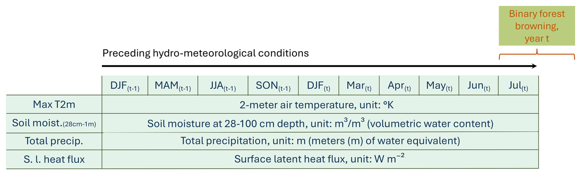
Figure 1 Predictors used to model binary forest browning in July–August of year t, based on 4 hydro-meteorological variables across 10 seasonal and monthly time periods. Each row represents one variable, and each column corresponds to a time step (seasonal or monthly anomaly), resulting in 40 potential predictors. The hydro-meteorological variables include: maximum 2 m air temperature (Max T2m), soil moisture at 28–100 cm depth (Soil moist. (28–100 cm)), total precipitation (Total precip.), and surface latent heat flux (S.l. heat flux). Time steps include seasonal means before the growing season (DJF: December–February, MAM: March–May, JJA: June–August, SON: September–November of the previous year (t−1); DJF: December–February of the same year t) and monthly means during the growing season (March, April, May, June, July). Units for each variable are indicated on the corresponding rows. Note that all predictors used in the random forest model are unitless, as the variables have been transformed into standardized monthly and seasonal anomalies, as detailed in Sect. 2.3.

With the term “predictor”, we refer to each variable at every given time step. Consequently, there are 40 potential predictors in total, as presented in Fig. 1.

2.4 Aggregating data for longer time series

The binary forest browning, our predictand, is a time series of 41 data points between 1981 and 2022, which is too short for a robust estimation of the statistical link between predictors and predictand. Therefore, we artificially create longer time series using the large amount of available spatial data. The 25 time series of GPs located in the same 0.5° × 0.5° grid box are stacked temporally by assuming that hydro-meteorological conditions triggering browning are the same for neighboring GPs (see Fig. C2 in the Appendix). We thereby obtain longer time series, up to 1025 data points (25 × 41) for each sub-region. Note that 1025 is the maximum length, which is obtained only if the 25 GPs are forest GPs (as defined in Sect. 2.2), with sufficient data quality for every summer (as specified in Sects. 2.1 and 2.2). For a robust statistical fitting, we discard stacked, balanced time series shorter than 80 data points (i.e., 0.5° × 0.5° boxes comprising less than two 0.1° × 0.1° forest GPs).

3 Method

3.1 Random forest

A large number of predictors (40, see Sect. 2.3) are here used as potential candidates to explain forest browning. To identify the most important predictors and their link to forest browning, we employ a random forest (RF) model (Breiman, 2001). The principle of the RF model is to compute a large number of decision trees, each fitted with a random sub-selection of the initial data, to assess the average link of each predictor with the predictand (here: binary forest browning) and its importance compared to the other predictors. We use 300 decision trees and 3 predictors per tree. These hyperparameters are found to be a good trade-off between performance and computation time (not shown). Moreover, using a low number of predictors per tree helps reduce the dominance of correlated variables in the model (Strobl et al., 2008; Gregorutti et al., 2013). We randomly divide the time series into a training subsample (75 %) and a testing subsample (25 %). The training data is used to both fit the RF model and calibrate the cutoff level of the RF output, to assign a probability of browning of “0” (no browning) or “1” (browning), and to compute the critical success index on the testing data (see the following Sect. 3.2).

The years with forest browning represent extreme conditions and are rare by definition. For the majority of grid points (GPs), less than 15 % of the years are “1”s (see Fig. B4 in the Appendix), while the remaining years are considered normal (“0”), indicating no significant browning. To improve the performance of the RF model, we balance the training dataset by randomly discarding “0” years, ensuring an equal number (rounded up to the nearest ten) of “0” and “1” years per GP. This random removal of “0” years additionally breaks potential temporal autocorrelation induced by stacking time series temporally. Following this procedure, we obtain a RF model for 1059 GPs across Europe.

The output of the RF function includes the mean decreased accuracy, a measure of the predictor's importance. The mean decreased accuracy of a given predictor quantifies the loss in predictive performance when this predictor is not included in the decision tree.

We use partial dependence analysis to interpret the influence of single variables (Friedman, 2001; RDocumentation, 2024). A partial dependence plot shows how the average probability of observing a specific outcome (e.g., forest browning) changes with a single input variable. The mean probability is calculated across all observations for the other predictors. The partial dependence is computed using the following formula:

$$\stackrel{\mathrm{̃}}{f}\left(x\right)={\displaystyle \frac{\mathrm{1}}{\mathrm{2}n}}\sum _{i=\mathrm{1}}^n\left(\log \left({\displaystyle \frac{p_{\mathrm{1}}(x,x_{\text{iC}})}{\mathrm{1}-p_{\mathrm{1}}(x,x_{\text{iC}})}}\right)\right),$$

where x is the value of the predictor for which partial dependence is calculated, p₁ is the proportion of decision trees in the random forest that classify the input as belonging to class “1” (forest browning), and x_iC corresponds to all the other predictors in the training data, and n is the length of the training data. $\stackrel{\mathrm{̃}}{f}$ is calculated for all the values of x in the training data. A high $\stackrel{\mathrm{̃}}{f}\left(x\right)$ indicates that the value x for the chosen predictor is associated with a high probability of forest browning.

3.2 Performance

We measure the skill of the RF model applied to the testing data with the critical success index (CSI; Schaefer, 1990). The CSI is defined as $\text{CSI}=\frac{\text{TP}}{\text{TP}+\text{FP}+\text{FN}}$, where TP is the number of true positives (successfully predicted and observed low greenness events, Y_t=1), FP is the number of false positives (i.e., false alarms, the model incorrectly predicted a low greenness event) and FN is the number of false negatives (i.e., missed events, the model erroneously predicted Y_t=0). The CSI focuses on the predictive skill of the low greenness events, which is the quantity of interest in our analysis. The accurately predicted normal years (Y_t=0) are not considered. The CSI varies between 0 and 1, where a higher value indicates a better forecast. A CSI of 0.5 means that the model predicted as many TP as the sum of FP and FN.

To assess the performance over all cut-off levels (see Sect. 3.1), we additionally compute the AUC, that is the area under the receiver operating characteristic (ROC) curve (Swets, 1988). The ROC curve displays the true positive rate versus the false positive rate against all cutoff levels. The AUC varies between 0 and 1, where values close to 0 indicate systematically incorrect predictions, values around 0.5 suggest performance that is not better than random guessing, and values higher than 0.5 indicate increasingly good predictions.

3.3 LASSO regression

We additionally run a LASSO logistic regression (Tibshirani, 1996) with the same predictors, predictand, training, and testing data as for the RF. Vogel et al. (2021) demonstrated that LASSO regression shows good performance in identifying meteorological drivers of extreme events (low wheat yield in their study). Therefore, we employ the LASSO logistic regression as a benchmark for the predictive skill. The penalty factor on the coefficients norm (λ_1se in Vogel et al., 2021) is obtained with a 10-fold cross-validation.

4 Results

4.1 Performance

As a first step, we evaluate the performance of the random forest (RF) classification model at predicting low-greenness events from the hydro-meteorological predictors (i.e., from the aforementioned variables and time periods, Fig 1). When applied to the testing data, the RF model exhibits excellent predictive performance for forest browning over Europe (see Fig. 2): 99 % of the GPs have a CSI greater than 0.5 (Fig. 2a). In other words, for 99 % of the grid points (GPs), the model predicts at least as many true positives (TP) as the sum of false positives (FP) and false negatives (FN). 65 % of the GPs have a CSI greater than 0.75 (i.e., at least 3 times as many TP as the sum of FP and FN). The AUC also indicates a good performance, with 98 % of the GPs having an AUC greater than 0.8, and 48 % of the GPs with an AUC larger than 0.95. The high AUC proves that the good performance does not depend on the cutoff level. In other words, the true positive rate is much higher than the false positive rate for all cutoff levels between 0 and 1.

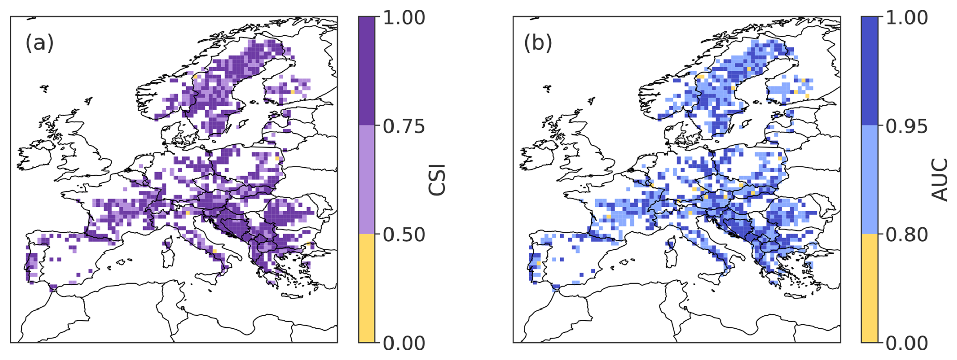
Figure 2 Spatial distribution of performance metrics for the random forest model: (a) CSI (critical success index) and (b) AUC (area under the ROC curve, both defined in Sect. 3.2) of the random forest model, evaluated with the testing dataset. Higher CSI and AUC values indicate better model performance.

There is no specific region showing a lower skill. The Balkans and Sweden exhibit particularly large areas of high skill, for both metrics. We do not observe a dependence between model performance and the percentage of forest cover within the GP area (not shown). This supports the use of a 10 % threshold for forest pixel inclusion, which ensures sufficient representation of forested pixels while maintaining broad spatial coverage.

When aggregating GPs temporally to obtain longer time series, we formulate the hypothesis that the neighboring 0.1° × 0.1° GPs in a 0.5° × 0.5° grid box are driven by the same predictors. The high skill of the RF, in terms of both CSI and AUC, confirms that this hypothesis is sound.

In comparison to the RF, the LASSO model exhibits a lower CSI for 83 % of the GPs, and a lower AUC for 89 % of the GPs (see Figs. E1 and E2 in Appendix). Only 92 % of the GPs exhibit a CSI greater than 0.5 for the LASSO model (99 % for RF). For the LASSO model, 45 % of the GPs attain an AUC above 0.9 (82 % for RF). An advantage of the LASSO logistic regression is the simple, linear link between predictors and predictand. This simplified link is outperformed by the RF model, allowing for flexible non-linear relationships between predictors and predictand.

4.2 Important drivers of forest browning

4.2.1 Example for two grid points

As an illustration of the RF model output analyzed in this study, we present the mean decrease accuracy and the partial dependence plots for two GPs in Europe highlighted in red in Fig. D1. These GPs were selected to showcase the diversity in forest type and the variability in driver responses captured by the RF model. The first grid point, predominantly broadleaf forest, is located in northeastern France and has 41 % forest cover. The RF model achieves a CSI of 0.92 and an AUC of 0.99 at this location. The second grid point, characterized by coniferous forest, is situated in southwestern Sweden, with 66 % forest cover, a CSI of 0.97, and an AUC of 1.

For the broad-leaved GP in the Jura forest in France, the low greenness events are largely explained by the hydro-meteorological conditions during the preceding year, especially the conditions in spring and summer (Fig. 3, grid point A). The most important variables include 2 m temperature (4 out of the 10 top predictors), soil moisture (3 out of 10), total precipitation, and surface latent heat flux (Fig. 3, left panel). Positive 2 m temperature anomalies in the summer of the preceding year and in July of the current year (left side of the x axis), as well as negative precipitation anomalies in MAM of the previous year (right side of the x axis), are all associated with an increased probability of forest browning (Fig. 3, grid point A, second, third, and last panels). These results suggest that summer heatwaves, occurring either during the growing season of the previous year or the current year, and dry conditions in the preceding spring are detrimental to forest health at this grid point.

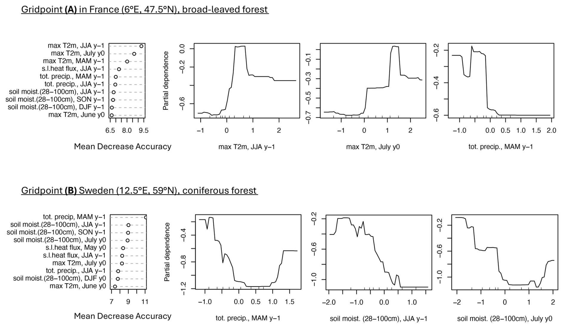
Figure 3 Example of predictor mean decrease accuracy and partial dependence for forest browning at two selected grid points. First column: 10 most important predictors (y axis), i.e., predictors with the largest mean decrease accuracy (x axis) for a grid point in broad-leaved forests in France (A) and a grid point in coniferous forests in Sweden (B) (location indicated in Fig. D1). Second, third, and fourth columns: partial dependence of forest browning (y axis) on the predictor's anomalies (x axis), for the three most important predictors. The mean decrease accuracy and partial dependence plots are introduced in Sect. 3.1.

For the coniferous GP in Sweden (Fig. 3, grid point B), the low greenness events are largely explained by the hydro-meteorological conditions during spring and summer of the same year and the preceding year. As for the France GP, soil moisture is particularly important (4 predictors out of the 10 most important). The four most important variables are precipitation in spring of the preceding year, soil moisture in July of the same year, and spring and fall of the preceding year (left panel of Fig. 3). The link between total precipitation in spring of the previous year and forest browning is non-linear: both positive and negative anomalies are associated with a higher probability of browning, although the impact of dry conditions is considerably stronger (Fig. 3, grid point B second panel). The same non-linear signal is observed for soil moisture in July of the same year (Fig. 3, grid point B in the last panel). Dry soil conditions in the summer of the preceding year increase the probability of forest browning at this GP (Fig. 3, grid point B in third panel).

The ranking of the top 10 predictors should not be interpreted too rigidly, as the differences in mean decrease accuracy are relatively small, and hence several variables may carry similar levels of explanatory power.

4.2.2 Results over Europe

To summarize the model results for all GPs over Europe, we display, for each predictor, the percentage of GPs over Europe that selected this predictor as one of the ten most important predictors in the RF model (Fig. 4A). The time period with the strongest influence on forest browning is spring and early summer of the considered year, especially for maximum 2 m temperature and soil moisture. In particular, the most frequently selected predictor is maximum 2 m temperature in June and July, with 57 % and 50 % of the GPs, respectively, retaining these predictors as one of the 10 most important ones. Soil moisture in July is retained as one of the 10 most important predictors for 43 % of the GPs. Additionally, 35 % of the GPs retain total precipitation in June as an important predictor. We observe a small signal of long-term impact of the preceding year in spring for maximum 2 m temperature (40 % of the GPs).

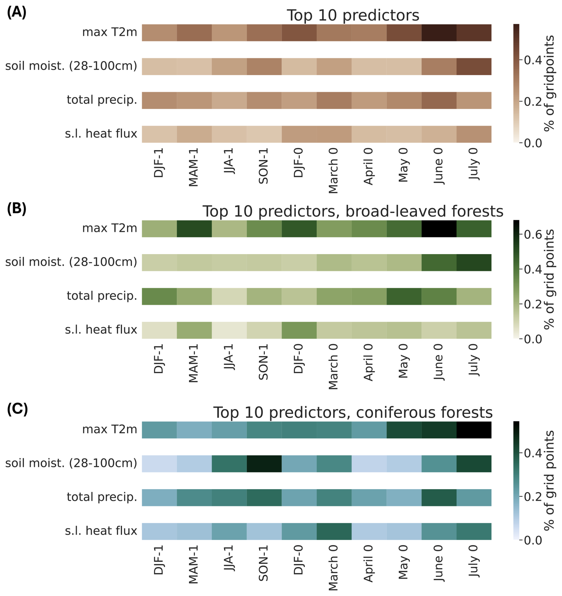
Figure 4 Importance of the predictors for all forest grid points. Each cell represents one predictor presented in Fig. 1, i.e., a given variable (y axis) for a specific time period (x axis). The color shading of each cell indicates the percentage of grid points where this predictor ranks among the top 10 most important predictors in the random forest model. The percentage is calculated for (A) all forest grid points over Europe, (B) broad-leaved forest grid points only, and (C) coniferous forest grid points only.

For the broad-leaved forests (see Fig D1 for forest type classification), the most selected predictor is maximum 2 m temperature in June of the year of the browning (166 GPs, i.e. 68 % of the broad-leaved GPs, Fig 4B). Except for one GP, the ensemble of partial dependence plots shows two clear plateaus, separating negative and positive temperature anomalies, indicating that above-average June temperatures are associated with an increased probability of forest browning (Fig. 5A, first panel). For the second most selected predictor, soil moisture in July of the year of the browning (for 93 GPs, i.e., 52 % of the broad-leaved GPs), the partial dependence plots also exhibit two plateaus, with dry conditions being associated with forest browning (Fig. 5A, second panel). Soil moisture in June and total precipitation in May and June of the same year also play a role for more than 35 % of the GPs (Fig 4B). In addition, there is an influence of spring 2 m temperature conditions one year before (for 51 % of the GPs). While the dependence on conditions in June of the same year is rather homogeneous, the link between forest browning and maximum 2 m temperature in spring of the preceding year changes slightly with latitude (not shown). Warm spring conditions in the preceding year negatively impact forests at higher latitudes, whereas cold spring conditions are detrimental to forests at lower latitudes.

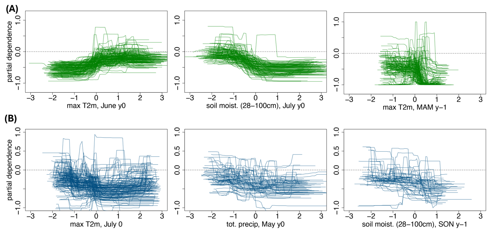
Figure 5 Partial dependence of forest browning (y axis) with a given predictor anomalies (x axis), for broad-leaved forest (A) and coniferous forest (B). The predictors are (A) maximum 2 m temperature and soil moisture (28–100 cm depth) in July of the same year, and maximum 2 m temperature in spring of the preceding year, for broad-leaved forests only and (B) maximum 2 m temperature in July of the same year, total precipitation in May of the same year and soil moisture (28–100 cm depth) in autumn of the preceding year, for coniferous forests only. For each dependence plot, we display only the grid points for which the predictor is among the top 10 predictors. The partial dependence plot is introduced in Sec.3.1.

The spring and early summer conditions before the studied summer are important predictors for coniferous forest browning (Fig. 4C). The most selected predictor is maximum 2 m temperature in July (150 GPs, i.e., 54 % of the coniferous GPs), followed by soil moisture in autumn of the preceding year (48 %), and in July of the same year (41 %). Total precipitation in June is selected as an important predictor for 37 % of the coniferous forest GPs, while surface latent heat flux in March is selected for 35 %. Compared to broad-leaved forests, the link between important predictors and coniferous forest browning is more heterogeneous (Fig. 5B). Surprisingly, some of the GPs at high latitudes show that negative anomalies of maximum 2 m temperature in July are associated with a higher probability of forest browning, whereas the same conditions are associated with a higher probability of browning at lower latitudes (not shown). Negative anomalies of soil moisture in autumn (i.e., dry conditions) are associated with a higher forest browning probability. The link with soil moisture in June of the same year is non-linear for some GPs and overall very dependent on the GP, making a generalization over the region tricky. However, there is a slight indication that negative soil moisture anomalies may be linked to a higher probability of forest browning.

We now examine the spatial distribution of the most influential predictors across Europe, highlighting regional patterns in predictor importance (Fig. 6). Temperature is selected as one of the top 10 most important predictors for the vast majority of GPs across Europe, with a few exceptions in Scandinavia and Bosnia and Herzegovina (top left panel). Soil moisture (28–100 cm) is not retained as an important variable in Switzerland, Eastern France, and the Northern Balkans, but it is selected in regions such as southern Iberia, the southern Balkans, and parts of Norway (top row, second panel). Interestingly, precipitation is also identified as an important predictor in Scandinavia, alongside soil moisture, and in some GPs in Central Europe where soil moisture is not retained. In contrast, surface latent heat flux does not emerge as a dominant predictor in any specific region; its importance appears relatively evenly distributed across Europe (Fig. 6, left and middle panels).

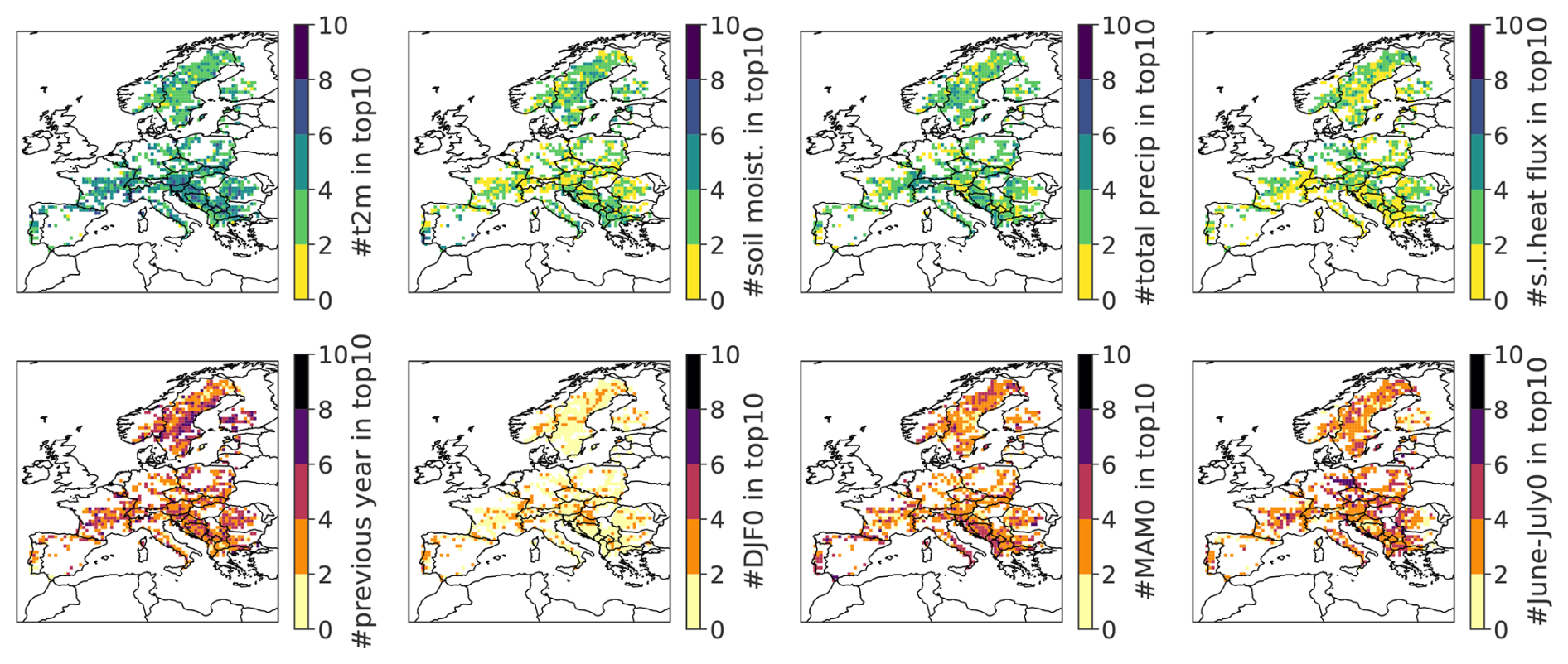
Figure 6 Spatial distribution of the relative importance of predictor types across Europe. At each grid point, the color indicates the number of times specific features appear among the top 10 most important predictors for forest browning. The top row shows meteorological variables (from left to right): 2 m temperature, soil moisture (28–100 cm), total precipitation, and surface latent heat flux. The bottom row displays temporal features (from left to right): seasonal averages from the previous year (DJF, MAM, JJA, SON), DJF of the current year, MAM of the current year, and June–July of the current year.

Temporal variables from the previous year are among the top 10 predictors at most GPs, with slightly higher importance observed at higher latitudes, particularly in Scandinavia (Fig. 6, bottom row, left panel). Similarly, conditions during June–July of the current year are frequently selected, with especially high importance in central France and eastern Germany, where between 6 and 8 of the top 10 predictors correspond to this period (bottom row, right panel). DJF of the current year plays a moderate role, being selected in GPs scattered across Europe (bottom row, second panel). Finally, spring conditions (MAM) of the current year are highly influential, with 4 to 6 predictors among the top 10 in several regions, including southern Italy, Portugal, central France, the Balkans, and Scandinavia (bottom row, third panel).

Altogether, the sub-seasonal to seasonal conditions of temperature, precipitation, and soil moisture in spring and early summer are the most important features to explain summer forest browning in Europe (Fig. 4). Soil moisture and precipitation offer complementary insights, with each variable emerging as important in different regions, highlighting distinct hydrological influences on forest vulnerability across Europe. The more relevant captured conditions for low greenness events in broad-leaved forests are hot and dry conditions in spring and early summer (of the same year or the preceding year). Higher than average summer temperatures are also among the most adverse conditions for coniferous forests, with exceptions depending on the GP. The temperature and moisture conditions in spring, summer, and autumn in the preceding year also contribute to predicting the summer browning of the forests, although their influence is smaller than that of the conditions in the same year.

5 Discussion

5.1 Identified adverse conditions

In this section, we examine the key hydro-meteorological drivers associated with low greenness events identified by our models and compare these findings with the existing literature to contextualize and validate our results.

Our model identified dry and hot conditions as adverse conditions for European broad-leaved forests, i.e., high temperature and low soil moisture (Figs. 3A and 5A), agreeing with existing literature (Rita et al., 2019; Beloiu et al., 2022; Rubio-Cuadrado et al., 2018; Senf et al., 2020; Knutzen et al., 2025; Schnabel et al., 2023). Temperature and moisture conditions in spring and winter of the preceding year also play a role, though to a lesser extent than conditions in the same year. Broad-leaved forests are predominantly located in the central and southern parts of Europe (Fig. D1), which are often water-limited during the growing season, with an increasing trend of drought frequency (Vicente-Serrano et al., 2014; Gudmundsson and Seneviratne, 2016; Rita et al., 2019). In warm conditions, trees increase evapotranspiration to cool the leaves. But when water is no longer available in the soil, stomata closure, at least during the warmest hours, is their only solution. It means that the tree cannot absorb CO₂ anymore, and photosynthesis is no longer possible. Resulting carbon starvation weakens the tree's defenses against herbivores, increasing the risk of tree mortality (see e.g. Gharun et al., 2024). Broad-leaved forests in Central and Southern Europe are particularly sensitive to water availability in May–July (Figs. 5 and 6), as previously observed by dendrochronology (Scharnweber et al., 2011; Rukh et al., 2023). Water availability for trees originates from both precipitation and soil reserves, which are typically replenished during spring and winter. Low precipitation in May can lead to dry soil conditions in June or July, limiting water availability during critical growth periods. This insufficiency becomes particularly problematic when a heatwave occurs in July, further increasing water demand. The detrimental effects of heatwaves in the preceding spring can arise from several factors: reduced growth or diminished reserves in the previous year, which leave trees weakened; a slow recovery rate following earlier stress events; or the physiological cost of a significant mast fruiting, which often follows warm summers in Fagus sylvatica (Leuschner, 2020).

The observed link between dry conditions (July) and warm conditions (May–July) and the increased coniferous forest browning probability (Figs. 3B and 5B) may similarly be linked to drought stress, facilitating bark beetle infestations on Picea abies and Pinus sylvestris (Dobbertin et al., 2007; Müller et al., 2022). In stressful conditions, conifers' fitness decreases, directly impacting resin production and thus the capacity to control insect infestation (Netherer et al., 2024). Moreover, warm conditions accelerate the reproduction rate of the insects and increase the number of generations in the same summer (Wermelinger et al., 2008). The link between July temperature and coniferous forest browning is rather heterogeneous over Europe. For low latitude grid points, the association between forest browning and warm July temperature aligns with the fact that dry and hot conditions are adverse conditions (Senf et al., 2020; Müller et al., 2022). For high latitude coniferous forests, a possible explanation for the association between cold July temperatures and low greenness could be related to frost damage. Frost damage is well documented in winter, particularly when the soil remains frozen for extended periods (Kullman, 1989, 1996), but summer frost events have not been widely reported or studied. Nevertheless, a strong decrease in productivity was observed during long cold spells in summer in Scandinavian pine forests (Matkala et al., 2021). Similarly, the observed increase in browning following dry soil conditions in the previous autumn (September–November) is not easily explained by existing studies or known physiological processes. One possible explanation is that drought stress during the hardening phase may impair nutrient uptake, weakening trees before winter. Alternatively, a deficit in soil moisture during autumn may persist into spring, limiting water availability at the onset of the next growing season. Additional research is needed to better understand the processes driving these associations.

Although precipitation anomalies are known to be significantly linked with forest browning (Hermann et al., 2023), this variable has a relatively low explanatory power to predict low NDVI in our model, compared to soil moisture, for example (Fig. 4). While precipitation and soil moisture are correlated, soil moisture may provide persistence information that precipitation does not. Another possible explanation is that large areas of forest at the European scale are located in flat areas with large water reserves or an available groundwater table. Hence, the reaction of forests to long droughts is potentially more correlated to soil water content than to precipitation. This result highlights the added value of an automatic procedure to select the most important features among a large set of potentially important variables.

Using the random forest model, we also established a statistical link between forest browning and hydro-meteorological conditions during the preceding year, hinting towards a source of inter-annual predictability for European forests. Two processes can explain this signal. First, when dry conditions occur in spring or summer and are not followed by sufficient rainfall in the subsequent months, the next growing season may begin with reduced soil water reserves, increasing the risk of drought-induced browning. Second, forests impacted by anomalous hot and dry summer conditions are more sensitive to adverse conditions during the following year (Brun et al., 2020; Frei et al., 2022). Consecutive years with adverse conditions may reduce tree resilience, indicating a “memory effect” (Anderegg et al., 2015; Hermann et al., 2023). A causality analysis (see e.g. Peters et al., 2017) could explore the role of the forest state for preceding summers or insect infestations as predictors, although this framework is beyond the scope of our study.

5.2 Preprocessing and predictor selection

We here discuss the choices and methodological considerations that guided our preprocessing and predictor selection steps, aiming to ensure comparability, reduce redundancy, and enhance the interpretability of model outputs.

To ensure comparability across predictors, we standardized all hydro-meteorological variables by removing the mean and dividing by the standard deviation. While we acknowledge that some variables (e.g., precipitation) are typically not normally distributed, particularly at daily scales, aggregation to monthly and seasonal means reduces skewness and tends to produce distributions closer to normal, in line with the Central Limit Theorem. Our goal was not to enforce normality but to center and scale variables consistently for model interpretation.

We excluded soil temperature as a predictor from the analysis, as its variability is driven by air temperature, which is already a predictor in our model. We also discarded snow water equivalent for a better comparison between regions, as this variable may be relevant only in snowmelt-driven catchments. We hypothesize that the precipitation and temperature predictors contain the information that snow water equivalent would bring, and that soil moisture, at least in flat areas, is partly dependent on snow melt. We did not consider windstorms, focusing on long-term, large-scale forest browning. Storm damage, though potentially extreme, is more localized (Hermann et al., 2023) and should be assessed with higher resolution NDVI datasets (Giannetti et al., 2021).

We removed long-term trends from the NDVI and hydro-meteorological variables to focus on interannual variability rather than gradual climate change. This procedure allows us to isolate the statistical relationship between short-term anomalies and forest browning. While detrending reduces the influence of the mean climate trend, it does not eliminate the increased frequency of extreme events, which may still reflect underlying climate shifts and remain visible in the anomaly patterns.

To address potential multicollinearity among predictors, we applied a conservative variable selection approach by removing those with pairwise correlation coefficients greater than 0.4 or lower than −0.4. This step was taken to reduce redundancy while preserving ecological interpretability. Given our focus on identifying the top 10 most important predictors, rather than interpreting their exact ranking, we did not apply additional diagnostics such as the Variance Inflation Factor (VIF, Fox and Monette, 1992). While Empirical Orthogonal Functions can be effective in reducing collinearity (North and Wu, 2001), they transform variables into abstract components that are difficult to interpret ecologically. Additionally, applying EOFs individually across thousands of grid points would hinder comparability across regions. Nonetheless, we acknowledge the value of both VIF and EOF approaches for future studies aiming to refine predictor selection for local studies.

5.3 Dataset limitations

In this subsection, we discuss the limitations associated with the datasets used in this study.

The NDVI tends to saturate at high leaf area index (LAI) values, particularly in dense broad-leaved forests (Aklilu Tesfaye and Gessesse Awoke, 2021). Our compositing strategy, using the median value of the NDVI for 10 d, mitigates saturation and potential cloud contamination (Asam et al., 2023). An alternative is the kernel-based NDVI (kNDVI), which can address the saturation problem of the NDVI (Wang et al., 2023). However, kNDVI requires parameter tuning and kernel selection tailored to each use case, with these settings potentially varying across GPs. In addition, Wang et al. (2022) found no significant improvement between using the NDVI versus the kNDVI, likely due to the default kernel values not being universally applicable. The use of NDVI ensures consistency across locations, facilitating comparability across Europe while mitigating biases through median compositing. While other studies have explored vegetation dynamics using total reflectances, Synthetic Aperture Radar technologies (SAR, e.g., Flores-Anderson et al., 2025; Thonfeld et al., 2022) or indices like the Normalized Difference Water Index (NDWI, e.g., Sturm et al., 2022), we selected NDVI due to the long temporal coverage and high revisit frequency of the AVHRR sensor, which is essential for a robust statistical analysis across Europe.

Compared to point measurements, the NDVI has two main limitations: (1) it tends to underestimate drought impacts (Hoek van Dijke et al., 2023), and (2) it lacks sensitivity to underlying structural or physiological forest browning (Gazol et al., 2018). To address limitation (1), we use a binary definition of forest browning, focusing on the relative extremeness of low greenness events rather than their absolute magnitude. Regarding point (2), our aim is to conduct a continental-scale analysis, which is possible here thanks to the large spatial coverage of the AVHRR NDVI dataset. For smaller-scale operational forecasts, such as those for small-scale forest management, we recommend following our method but training the model on higher spatial resolution data. Such high-resolution data could include, e.g. station observations of hydro-meteorological data and forest field measurements, if these are available for sufficiently long periods. Additionally, we suggest using our verification method, with both CSI and AUC, to measure accuracy. Future local studies could also explore differences in browning dynamics and model performance between managed and unmanaged forest areas, such as protected zones, to better account for the influence of silvicultural practices not captured by land cover classifications alone.

Soil moisture from reanalysis datasets can present uncertainties due to sparse in-situ measurements and heterogeneous soil properties that influence local moisture dynamics. While these limitations are well-documented, including a potential underestimation in dry regions such as the Mediterranean during summer, Zeng et al. (2022) show that ERA5-Land soil moisture remains among the most reliable reanalysis products, with good agreement with observations. We chose ERA5-Land to maintain consistency across all climate variables used in the model. Moreover, we rely on soil moisture anomalies rather than absolute values, which helps reduce systematic biases and emphasizes relative changes over time. Although the quality of reanalysis data may influence model performance, the high predictive accuracy of the random forest substantially reduces concerns regarding its impact.

Our analysis identifies key variables for predicting low greenness events. These variables can be directly monitored using model output from ECMWF forecasts. While evaluating the predictive skill of various ECMWF forecast variables lies beyond the scope of this study since these datasets were not used, relevant literature on this topic is available (Zampieri et al., 2018; Krouma et al., 2024; Nicolai-Shaw et al., 2025; Recalde-Coronel et al., 2024).

6 Conclusion

In this study, we presented a large-scale, spatially explicit identification of forest browning drivers across Europe, using a homogeneous and fully automated modeling framework. Our approach achieves high predictive performance while running independent models for each 0.5° grid point, enabling a regionally nuanced comparison of hydro-meteorological drivers. We used the AVHRR NDVI data, which spans a temporal range of 41 years, to capture the state of European forests during summer. We used the fine spatial resolution of the AVHRR data to create a sufficiently long time series for conducting a random forest (RF) classification. The high CSI indicates that, given a cutoff level (that assigns a probability of browning to a “0” or a “1”), the model accurately predicts low-greenness events more often than missing an extreme or producing a false alarm. The high AUC indicates that the performance does not depend on the cut-off level. Our model demonstrates a high predictive score and is sufficiently general to compare the link between drivers and forest browning across all grid points in Europe.

We show that the most essential time periods to predict summer browning are primarily spring and early summer preceding the studied summer. Temperature and soil moisture conditions in spring and early summer are the most important predictors of European summer forest browning. Additionally, temperature, precipitation, and soil moisture conditions from the preceding year also play a significant role, indicating a multi-year influence on forest health. This effect is particularly notable in Scandinavia, where previous-year conditions account for a substantial portion of the most important predictors.

For broad-leaved forests, hot and dry conditions in spring and early summer, both in the current and previous year, are strongly associated with browning events. In coniferous forests, the influence of past conditions is more heterogeneous, with spring, autumn, and winter of the previous year contributing to browning risk. Thanks to the flexible dependence structure of the random forest model, we also uncover non-linear relationships between hydro-meteorological variables and forest browning. For instance, both unusually high and low precipitation anomalies during spring of the previous year can be detrimental to coniferous forests.

The identification of critical conditions and time periods at the local scale, combined with the use of hydro-meteorological variables available from sub-seasonal to seasonal forecast products, offers practical opportunities for proactive forest management. Regional forest agencies can leverage our methods and findings to anticipate periods of increased risk and implement targeted preventive measures, such as monitoring key variables in preceding seasons and years (e.g., autumn soil moisture or spring temperature). This approach enables more strategic allocation of resources, including irrigation, thinning, or pest control, tailored to the most influential local drivers. Such preventive measures would mitigate the economic and environmental costs of forest damage.

Appendix A: AVHRR NDVI composites

To account for differences in the spectral response function (SRF) among the AVHRR sensors (AVHRR/1, AVHRR/2, and AVHRR/3), the data were normalized to NOAA-9 AVHRR/2 following the method described by Fontana et al. (2009) and Barben et al. (2024), using the polynomial coefficients proposed by Trishchenko et al. (2002). This SRF correction was applied to the entire LAC dataset, covering all of Europe. As demonstrated in both Fontana et al. (2009) and Trishchenko et al. (2002), the correction performs well across various biomes.

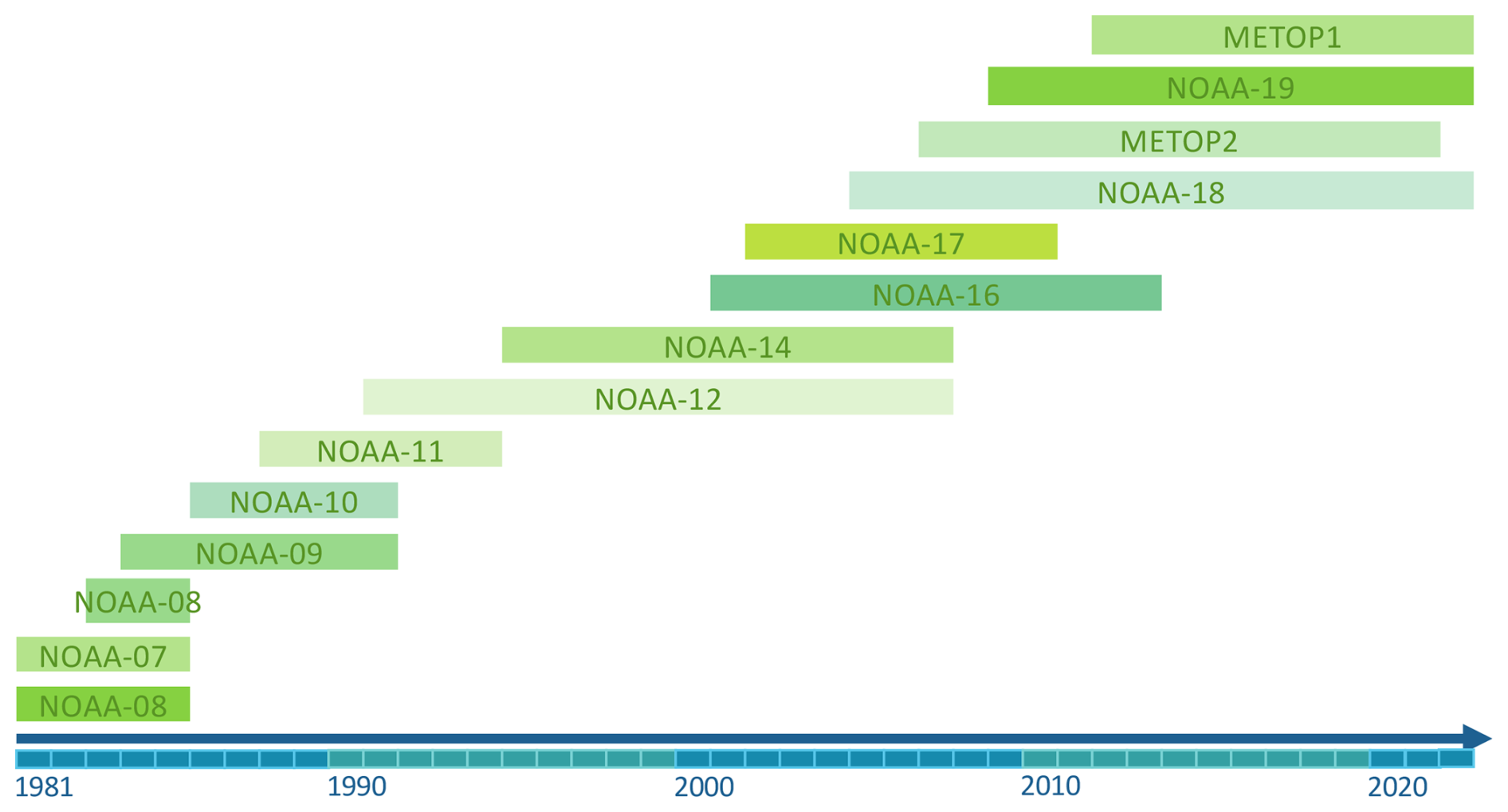
Figure A1 List of the satellites used for our study along with their years of data availability (x axis).

The 10 d AVHRR NDVI dataset (Dupuis et al., 2024) hosted at the University of Bern has been derived by computing the median NDVI values across ten consecutive days. Prior to the compositing, a cloud mask is applied to the single satellite image to filter out pixels contaminated by clouds. Each pixel in the AVHRR dataset was subject to quality control before computing the 10 d composites from the daily NDVI data. For a given observation, the pixel is masked out if the satellite viewing angle is higher than 55°. Additionally, the sun zenith angle must be below 80° for the observation to be considered valid. Similarly, if the cloud probability mask is above 30 % or the quality of the cloud mask is not qualified as “good”, then the pixel is masked out. We then compute the 10 d composite as the mean NDVI value for the valid days over the 10 d. The number of valid pixels used for the compositing generating is recorded, as well as the number of pixels exhibiting cloud probabilities between 1 % and 30 %. If fewer than two valid days are detected for a given 10-composites, the composite is set to missing data.

Appendix B: NDVI and forest browning

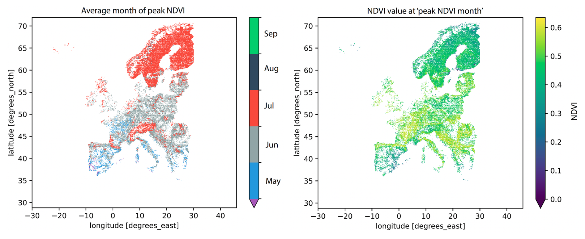
Figure B1 Spatial patterns of the average month of the NDVI peaks across European forest grid points (left panel) and mean value of the NDVI peak (right panel). The average month of yearly NDVI maximum is computed for each 0.1° forest grid point. Colors on the left panel indicate the month of peak NDVI: purple for April, blue for May, grey for June, red for July, navy blue for August, and green for September.

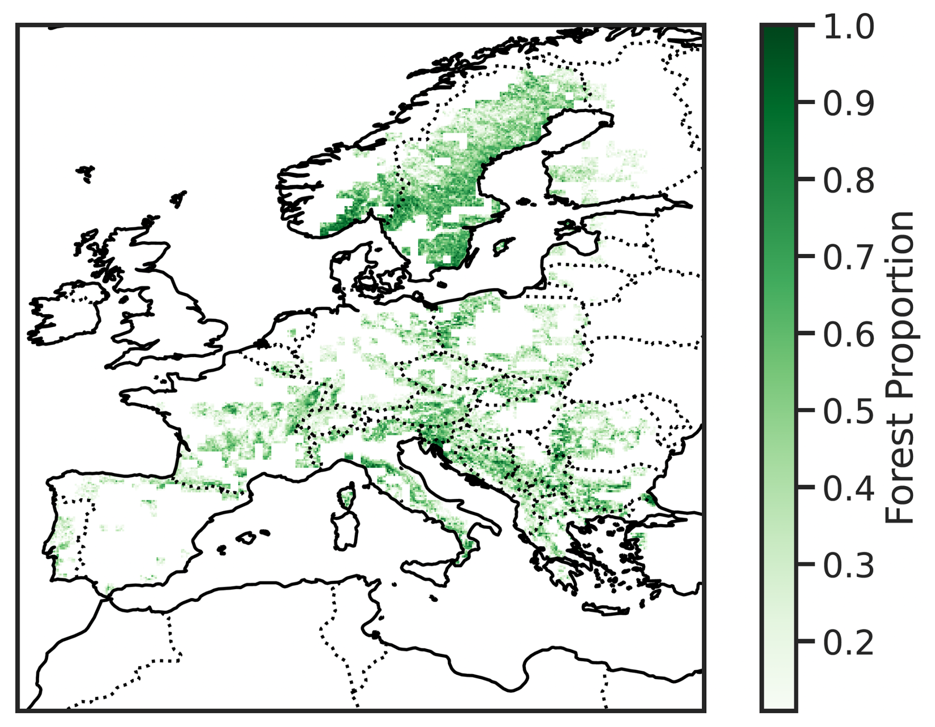
Figure B2 Percentage of forest cover within each 0.1° × 0.1° grid cell, based on CORINE land cover classification. Percentages are computed from underlying 0.01° resolution pixels, and only grid cells with more than 10 % forest coverage are displayed.

Figure B3 Time series of forest browning on a 0.1° × 0.1° grid, as defined in Sect. 2.2. A forest grid point is displayed in orange if it experiences a low-greenness event (Y_t=1, in Sect. 2.2), and in green for normal years (Y_t=0, in Sect. 2.2).

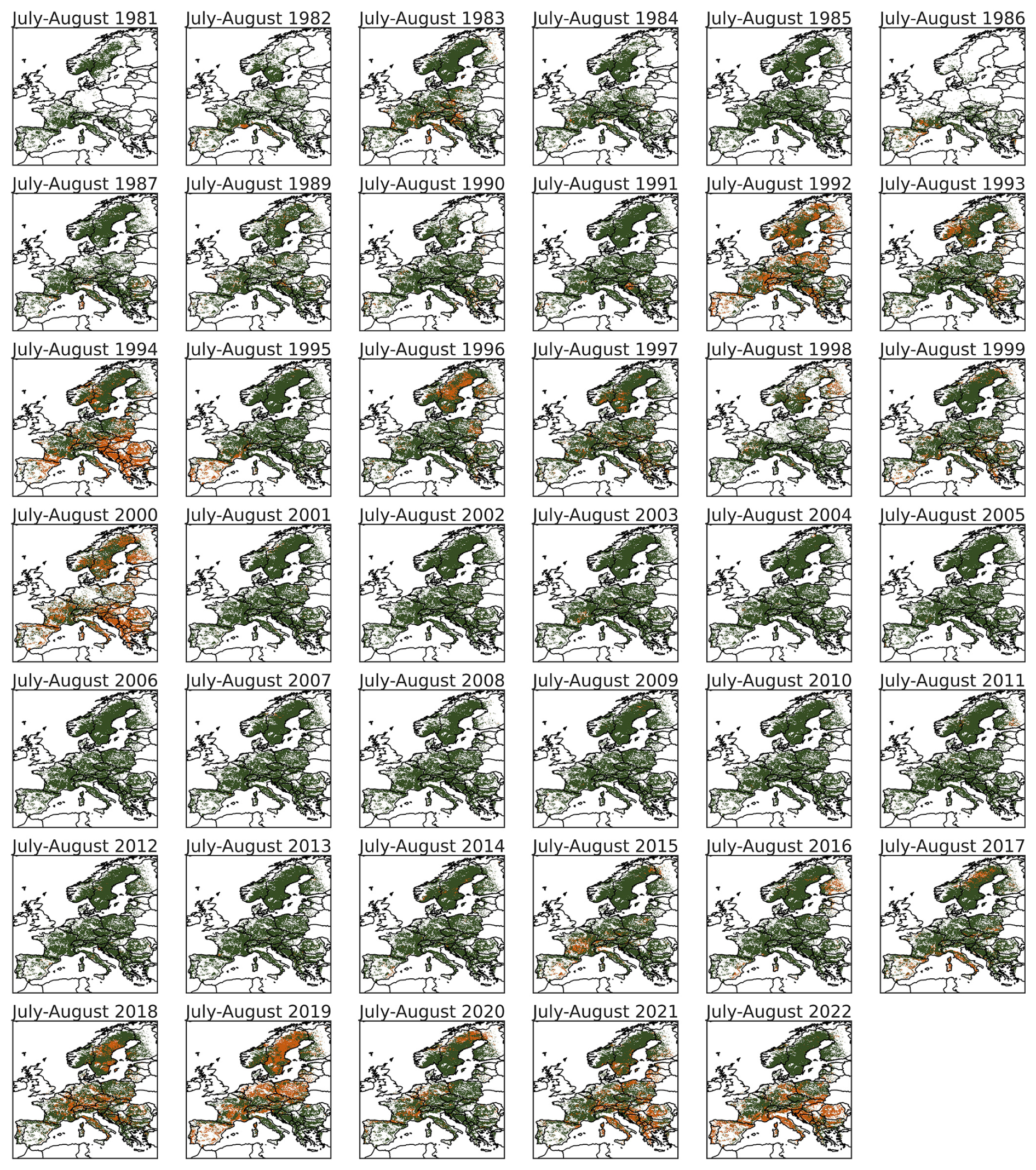
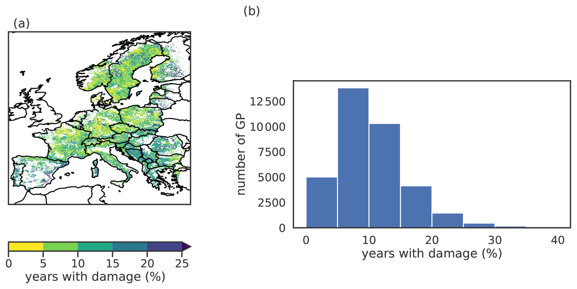
Figure B4 Proportion of years with forest browning. (a) Spatial distribution and (b) histogram of the proportion of years with forest browning (i.e., damage) for each grid point (GP) across the 0.1° grid. The binary forest browning is defined in Section 2.2.

Appendix C: Hydro-meteorological drivers and data processing

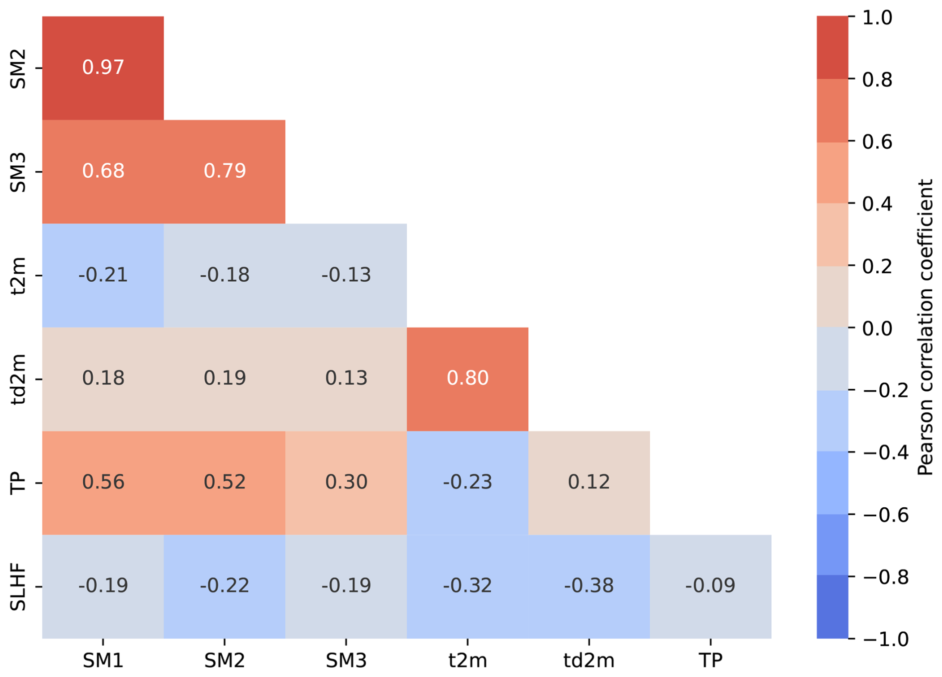
Figure C1 Pairwise correlation coefficients between hydro-meteorological predictor variables, averaged across months and over Europe. Variables include soil moisture at three depths (SM1: 0–7 cm, SM2: 7–28 cm, SM3: 28–100 cm), 2 m air temperature (t2m), 2 m dew point temperature (td2m), total precipitation (TP), and surface latent heat flux (SLHF). We excluded td2m, SM1, and SM2 from the analysis to ensure that all remaining predictors have cross-correlations between −0.4 and 0.4, thereby reducing multicollinearity and enhancing model interpretability.

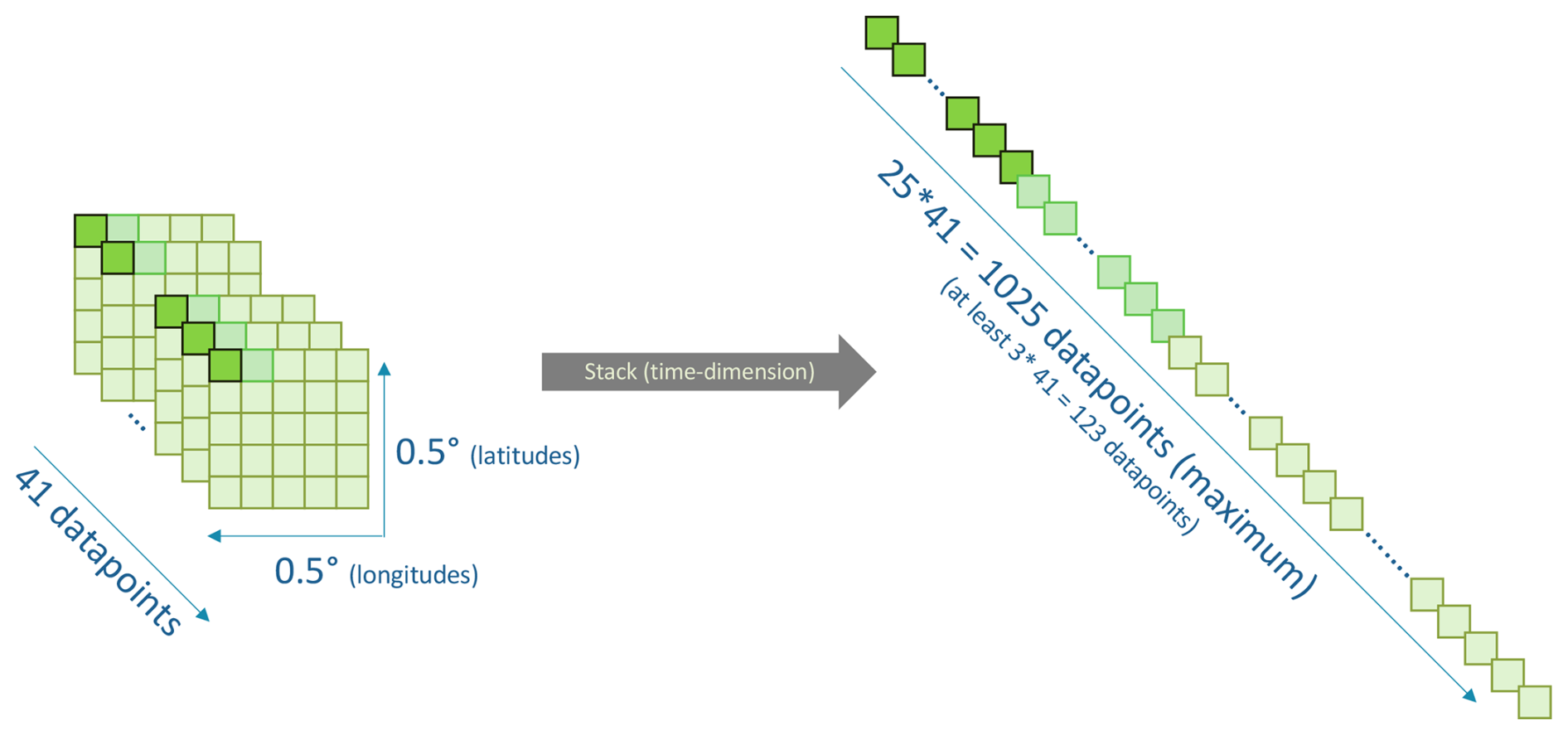
Figure C2 Schematic of the stacking procedure to obtain longer time series. All of the 0.1 × 0.1  orest GPs in a 0.5 × 0.5 box are stacked on the time dimension. The same procedure is applied for the preceding hydro-meteorological conditions, individually for each grid point.

Appendix D: Forest Type

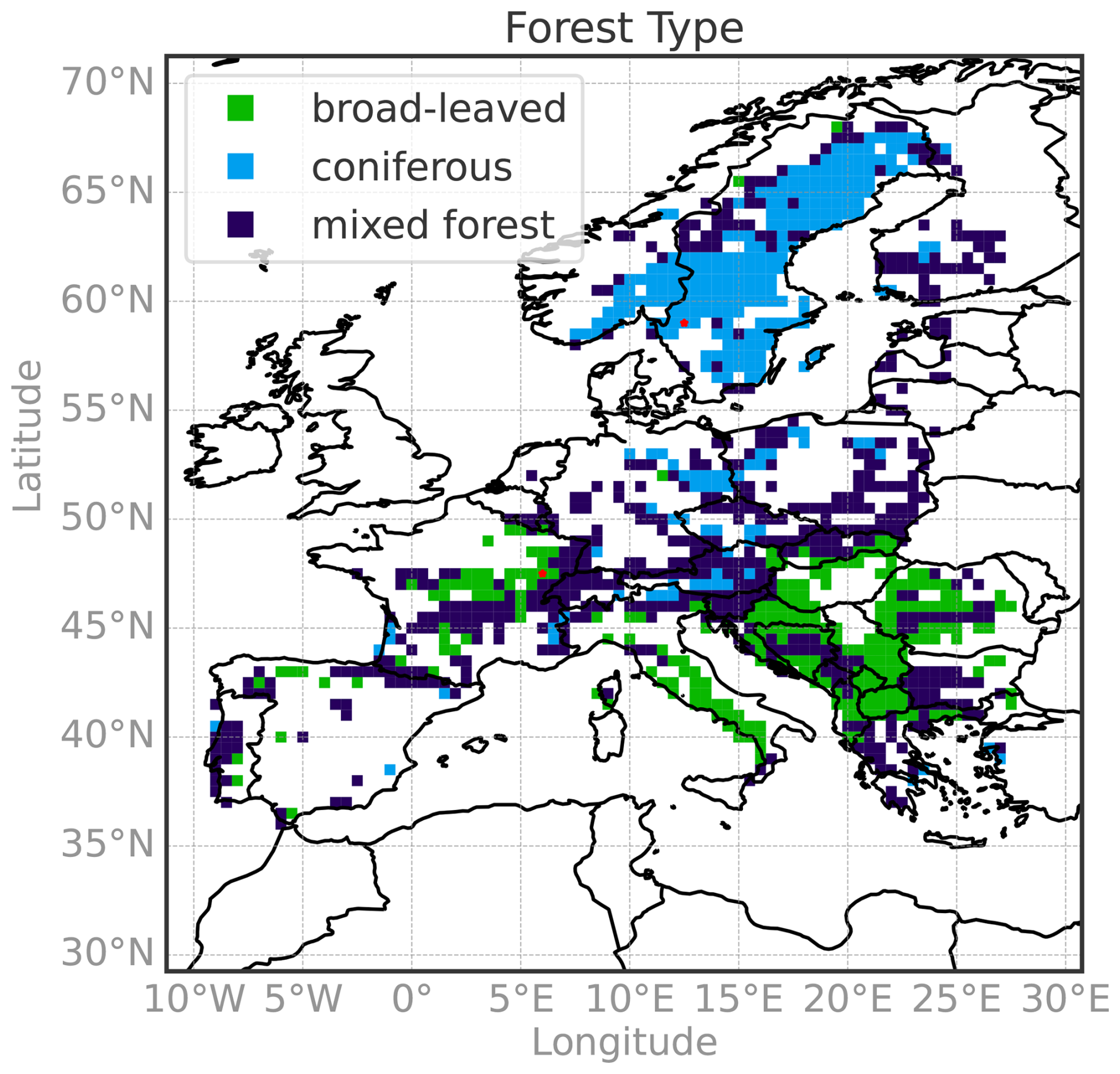
Figure D1 Forest type on the random forest model grid. Forest types across the 0.1° × 0.1° grid used for the random forest model output, based on CORINE Land Cover classification: broad-leaved forests, coniferous forests, and mixed forests. The model was applied to a total of 1059 grid points, including 244 broad-leaved forest points and 275 coniferous forest points. The two red stars indicate the locations of the grid points analyzed in Fig. 3.

Appendix E: Model performance

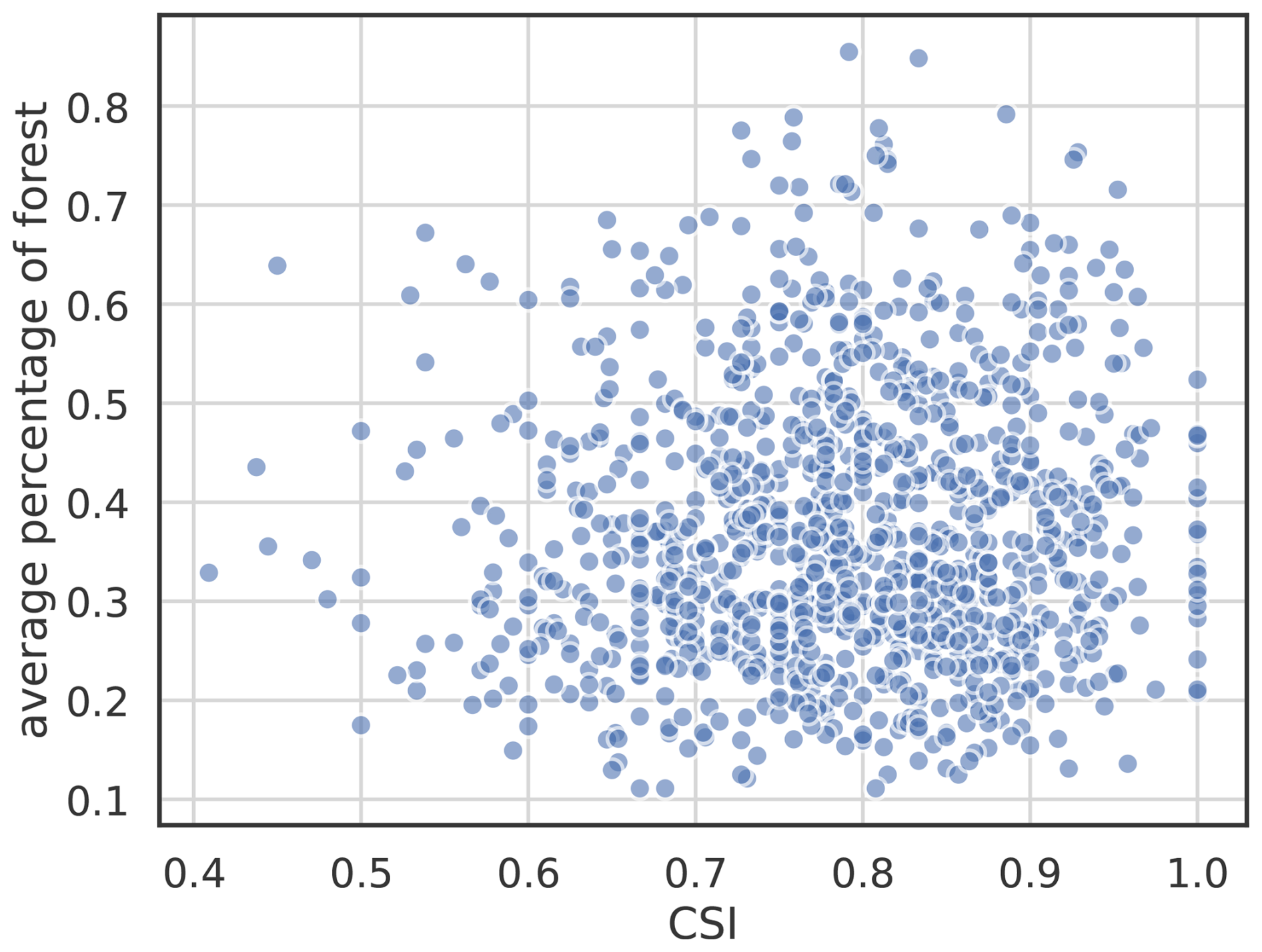
Figure E1 Scatterplot between the critical success index (CSI) of the random forest model and the percentage of forest for each 0.5° × 0.5° gridpoints.

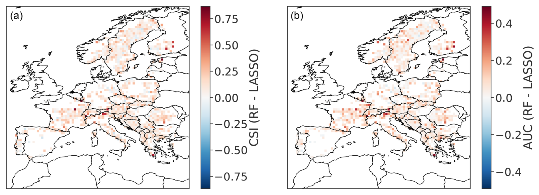
Figure E2 Spatial distribution of difference in performance metrics between the RF and the LASSO model: (a) CSI (critical success index) and (b) AUC (area under the ROC curve, both defined in Sect. 3.2), evaluated with the testing dataset.