Warnings based on risk matrices: a coherent framework with consistent evaluation

Risk matrices are widely used across a range of fields and have found increasing utility in warning decision practices globally. However, their application in this context presents challenges, which range from potentially perverse warning outcomes to a lack of objective verification (i.e. evaluation) methods. This paper introduces a coherent framework for generating multi-level warnings from risk matrices to address these challenges. The proposed framework is general, is based on probabilistic forecasts of hazard severity or impact, and is compatible with the Common Alerting Protocol (CAP). Moreover, it includes a family of consistent scoring functions for objectively evaluating the predictive performance of risk matrix assessments and the warnings they produce. These scoring functions enable the ranking of forecasters or warning systems and the tracking of system improvements by rewarding accurate probabilistic forecasts and compliance with warning service directives. A synthetic experiment demonstrates the efficacy of these scoring functions, while the framework is illustrated through warnings for heavy rainfall based on operational ensemble prediction system forecasts for Tropical Cyclone Jasper (Queensland, Australia, 2023). This work establishes a robust foundation for enhancing the reliability and verifiability of risk-based warning systems.

1 Introduction

Early warning systems are used globally to alert a range of users, including the general public, to act to reduce the potential for harm in advance of hazardous events (UNDRR, 2024). A key feature of many warning systems is the use of warning levels, which typically operate as a series of escalating categories used to communicate threat. Levels can be based on a range of information. Many warning levels are informed directly by the severity or urgency of a hazard (Neußner, 2021). For example, warnings from the German Weather Service (DWD) have four levels which correspond to increasing hazard strength (DWD, 2024). More recently, there has been a move by meteorological agencies toward impact-based forecasting (WMO, 2015), and many services now use levels to explicitly indicate escalating impact potential. The UK Met Office (UKMO) issues impact-based warnings with the highest level, “Red Warning”, corresponding to a very likely risk to life and substantial disruption (UK Met Office, 2024). This is an approach reflected by many emergency service agencies. For example, the warning system used in Australia matches the action required by the community to promote safety (AIDR, NEMA, 2024).

Determining when and at what level to issue a warning is a key decision ideally informed by a probabilistic assessment of possible outcomes made by a forecaster (or forecast system) in conjunction with well-defined criteria. Such criteria are known as “forecast directives” (Murphy and Daan, 1985) and should be determined in consultation with key stakeholders of the warning service. An example of a forecast directive for a warning service for damaging wind gusts is “Issue a warning if and only if the probability of a wind gust exceeding 90 km h⁻¹ is at least 10 %”. Historically, considerable effort has been invested to advise or recommend thresholds that define severity categories (Stepek et al., 2012). In recent years, probability or likelihood information has been increasingly incorporated into warning decision frameworks. This shift recognises the need for an appropriate degree of confidence before issuing a warning and is driven by a surge in probabilistic data following the advent of ensemble-based forecasting systems (Legg and Mylne, 2004). Over a decade ago, the UKMO pioneered the use of impact–likelihood matrices, an example of which is shown in Fig. 1, to communicate risk and generate warning levels for weather-related hazards in the United Kingdom (Neal et al., 2014; Hemingway and Robbins, 2020; UK Met Office, 2024). This approach has since been endorsed by the World Meteorological Organization (WMO, 2015) and is used by a number of other meteorological agencies (Indonesian Agency for Meteorology, Climatology, and Geophysics (BMKG), 2016; South African Weather Service, 2020; Barbados Meteorological Services, 2020). These “risk matrices”, which are widely used in a range of fields, have found increasing utility in warning decisions as they provide a simple process for determining the warning level based on the severity (or impact) and associated certainty (or likelihood) of the hazard. Ideally, the warning level increases as the hazard becomes sufficiently more severe and/or certain. When well-defined and coherent, such risk matrices can constitute a forecast directive for the warning service.

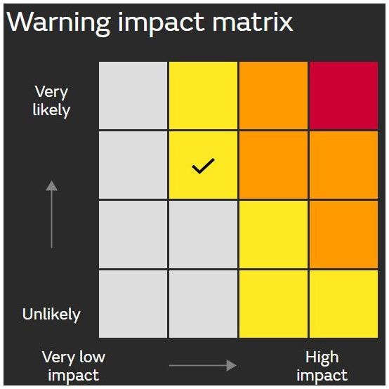
Figure 1 The warning impact matrix used by the UKMO (UK Met Office, 2024). In this example, a “Yellow Warning” level is issued, as indicated by the tick.

Despite their prevalence, serious problems have been identified with the conventional use of risk matrices in other fields (Cox, 2008; Ball and Watt, 2013). In the warning context, current operational risk matrix approaches also have problems, including situations where warning level decreases even as hazard likelihood increases, as discussed in Sect. 2.2. Furthermore, issues arise when categories are not well-defined, as is often the case with services based on impact or consequence, which are usually described qualitatively. When the warning decision process lacks adequate definition, two forecasters with identical probabilistic assessments of the hazard could issue two different warning levels. This may lead to warning messages that fluctuate unnecessarily, compromising both public safety and service credibility. Furthermore, it also limits verification (i.e. evaluation) of warning performance post-event. In fact, while the UKMO's impact-based warning system undergoes some subjective verification, objective verification is not conducted (Suri and Davies, 2021), and a recent attempt at more objective verification has encountered difficulties (Sharpe, 2024).

Warning verification is important for a number of reasons. Firstly, it enables agencies to monitor performance; compare the quality of different forecast systems; and implement targeted, evidence-based enhancements to improve service prediction (Loveday et al., 2024). Secondly, through objective verification, agencies can demonstrate their performance to users, thereby building trust. An indispensable tool for measuring the performance of warning accuracy, or for assessing whether a system upgrade will lead to improved prediction for a warning service, is a scoring function that is consistent for the prediction task at hand (Gneiting, 2011). A scoring function assigns a number to a forecast, which is a measure of how good the forecast was compared to the corresponding observation. In the context of warnings, a scoring function is consistent if the forecaster's expected score is optimised by following the forecast directive. The FIRM framework (Taggart et al., 2022) provides a family of scoring functions that are consistent for warning services that (1) have warning levels that correspond to severity categories and (2) use a measure of certainty based on either a fixed probability threshold or the severity category in which the expected value lies. The FIRM score has recently been used to recommend substantial predictive improvements to a heatwave warning service (Loveday and Carroll, 2025). However, for warning services in which the warning level is determined using a risk matrix, consistent scoring functions have not been available until now.

In this paper we present a general framework for determining warning levels using risk matrices. Unlike some warning systems based on risk matrices, our framework is coherent in the sense that the warning level cannot decrease if certainty and/or severity increases. This is achieved by requiring that the severity categories that represent warning conditions are well-defined and nested and that forecasters select a well-defined certainty category for each of these severity categories. We also present an extension to the framework that incorporates lead time to hazard onset into warning decisions. This provides greater flexibility in warning messaging and ensures compatibility with the Common Alerting Protocol (CAP) (OASIS OPEN, 2024).

The forecast directive for this framework is to fill out the risk matrix in line with the forecaster's probabilistic assessment of the hazard. We provide an accompanying evaluation framework that consists of a family of scoring functions that are consistent with the forecast directive. This evaluation framework encourages forecasters to follow the forecast directive, in the sense that their expected score is optimised by doing so. It also rewards forecasters who make superior probabilistic assessments. This promotes reliable warning decisions and improved hazard prediction. These consistent scoring functions are an extension of a special case of the FIRM score.

Our approach is hazard agnostic, meaning that it can be applied to any hazard or combination of hazards and can be extended to an impact-based service if desired and appropriate data are available. The framework and evaluation method applies equally well if the labels “warning level”, “severity” and “certainty” are replaced with “risk level”, “impact” (or “consequence”) and “likelihood” (or “probability”) respectively. It is also suitable for other areas of risk management, provided that the risk matrix itself represents an adequate model of risk for the application.

The paper is structured as follows. Section 2 presents the general warning framework, illustrated by a simple example for a heavy rainfall warning service. Section 3 describes the new consistent scoring method for warnings based on our general framework. Section 4 presents a case study illustrating the warning framework and verification approach using precipitation forecasts for Tropical Cyclone Jasper. Finally, Sect. 5 presents a summary and discussion of results.

2 Warning framework using risk matrices

In this section we lay out the general framework for determining a warning level based on a risk matrix assessment. Section 2.1 begins with a simple example to illustrate the main concepts, before laying out the general framework in plain language. Section 2.2 discusses key differences between our framework and the presentation of other frameworks, along with justification for our choices. Section 2.3 explains how the general framework can be extended to incorporate urgency, or warning lead time, into warning level determination. Section 2.4 then gives a mathematical description of the framework.

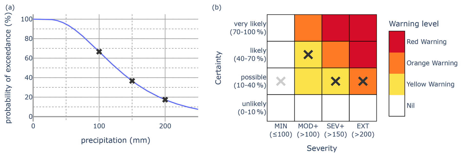
Figure 2 Example of a probabilistic forecast (a) for precipitation and its mapping (via dark grey crosses) to a severity–certainty matrix (b). The light grey cross indicates the certainty category for the MIN severity category implied by the probabilistic forecast. Severity thresholds, shown below the matrix, are in millimetres. In this case an Orange Warning would be issued.

2.1 Illustrative example and general framework

Consider a service that warns for heavy rainfall over a 24 h duration for Sydney, Australia. Figure 2b shows the risk matrix for this warning service. It is a 4×4 matrix with four certainty categories (unlikely, possible, likely and very likely) and four severity categories (MIN, MOD+, SEV+ and EXT, which correspond to severity outcomes that are negligible to minor, moderate or greater, severe or greater, or extreme). Each of the categories is clearly defined. An outcome is MOD+ (SEV+ and EXT respectively) if the 24 h rainfall exceeds 100 mm (150 and 200 mm respectively), while an outcome is MIN if the 24 h rainfall does not exceed 100 mm. A probability p is in the unlikely, possible, likely and very likely categories if $\mathrm{0}\mathit{\%}\le p<\mathrm{10}\mathit{\%}$, $\mathrm{10}\mathit{\%}\le p<\mathrm{40}\mathit{\%}$, $\mathrm{40}\mathit{\%}\le p<\mathrm{70}\mathit{\%}$ and $\mathrm{70}\mathit{\%}\le p\le \mathrm{100}\mathit{\%}$ respectively. The associated probability thresholds, or probability decision points, are p₁=10 %, p₂=40 % and p₃=70 %.

The warning service has four warning levels: Nil, Yellow Warning, Orange Warning and Red Warning. These are listed in order of increasing threat, and each level is paired with a colour (white, yellow, orange and red) of corresponding increasing intensity. Cells in the matrix are coloured to indicate the warning scaling, which is used to determine the level at which a warning is issued.

The forecast directive requests that the forecaster selects, for each severity category, the unique certainty category that aligns with their probabilistic assessment. By doing so they will select one cell in each column of the risk matrix. The warning directive requests that the forecaster follows the forecast directive and then chooses the warning level that is the highest warning level of the selected cells in the matrix.

For example, suppose that a forecaster has a predictive distribution for 24 h rainfall, shown by the probability of exceedance (PoE) curve in Fig. 2a. The forecaster's assessment is that the probability of exceeding 100 mm (i.e. observing a MOD+ outcome) is 66 %, which falls within the “likely” category. If the forecaster follows the forecast directive, they will select the “likely” cell in the MOD+ column of the matrix. The dark grey crosses in Fig. 2 show the probabilistic assessment of the forecaster and how this is mapped onto the matrix by following the forecast directive. The highest warning level from the selected cells is orange, and, therefore, following the warning directive, an Orange Warning will be issued.

The example above illustrates most of the key ingredients of this warning framework. These are the outcome space, the severity and certainty categories, the probability thresholds, the warning levels, the warning scaling, a forecast for the warning service, the forecast directive, the warning directive, and the evaluation weights. Each of these is described in more general terms below, with evaluation weights deferred to Sect. 3.

The outcome space is the set of all possible outcomes, which in the Sydney rainfall example would be all possible rainfall totals (in millimetres). The severity categories are categories of increasing hazard that together cover every possible outcome. The severity categories, excluding the first, are nested, so that in the Sydney rainfall example the set of outcomes in MOD+ includes those in SEV+, which in turn includes those in EXT. The first severity category (MIN) consists of all remaining possible outcomes, covering all events for which no warning would ever be issued. The certainty categories partition the probability space into categories of increasing likelihood, with corresponding probability thresholds. The warning levels are ordered from the lowest threat to the highest threat.

The warning scaling maps each cell in the risk matrix to a warning level. We adopt the standard risk matrix convention that severity categories (the columns) increase from left to right and certainty categories (the rows) increase from the bottom to the top. The warning scaling has three key properties: (a) the left column and bottom row are assigned the lowest warning level (Nil), (b) warning levels are non-decreasing moving from left to right along each certainty row, and (c) warning levels are non-decreasing moving from the bottom to the top along each severity column. Property (a) ensures that the warning service is not in a perpetual state of warning, while properties (b) and (c) ensure that any increase in the warning level (given a fixed warning scaling) is due to increased likelihood of the hazard, increased severity of the hazard or both.

A forecast for the warning service is the selection of one certainty category for each severity category (i.e. a cross in each column of the risk matrix). The forecast directive and warning directive have already been described. However, selecting a cell in the first column of the matrix will not affect the warning level (because the first column always gives the lowest warning level of Nil), so both directives will henceforth only require a categorical certainty forecast for all severity categories except the first. (In practice, forecasters may be encouraged to make a forecast in the first column for communication purposes.) While a forecaster need not follow the directives, one major contribution of this paper is to present an evaluation framework that encourages forecasters to do so.

Finally, note that the framework presented here is quite general. The number of severity categories, certainty categories and warning levels could be different from that illustrated with the Sydney rainfall example, as could the labelling of each of the categories or levels. It is also able to handle a variety of situations, including phenomena where hazards occur at either end of a spectrum and warnings for multiple hazardous phenomena. This is illustrated with the following two examples.

• (E1)

  A warning service for hazardous outdoor temperatures (either cold or hot) could define a MOD+ severity category as temperatures greater than 35 °C or less than 0 °C, a SEV+ severity category as temperatures greater than 40 °C or less than −5 °C, and an EXT category as temperatures greater than 45 °C or less than −10 °C.

• (E2)

  A warning service for large hailstones and/or damaging wind gusts in a 24 h period could define a MOD+ category as events where the maximum hailstone diameter is at least 20 mm and/or the maximum wind gust is at least 25 m s⁻¹ and a SEV category where the maximum hailstone diameter is at least 50 mm and/or the maximum wind gust is at least 35 m s⁻¹. There is no EXT category in this example.

More generally, the framework could be applied to an index, which itself represents complex multi-hazard interactions. An example of such an index is the Fire Behaviour Index (FBI) used in the Australian Fire Danger Rating System (AFDRS), which combines weather and fuel state information to determine the severity of fire behaviour (Hollis et al., 2024). Although we call the categories associated with columns “severity categories”, our general framework is also applicable to impact–likelihood matrices, where the outcome space is the set of possible impacts from the phenomena of concern.

2.2 Comparison with other warning schemes based on risk matrices

Several features of the warning framework merit further discussion as they differ structurally from some risk matrix warning tools proposed elsewhere or used by operational centres. A key comparison is with the work of the UKMO, to which the current authors are indebted. Although some of the labels are different (e.g. the UKMO warns for impact rather than severity), the essential structure of their matrix-based approach, shown in Fig. 1, can be translated to our representation in a straightforward manner. This is demonstrated in Fig. 3, where the matrix marked (a) conforms to our framework, while the matrix marked (b) is a translation of the UKMO matrix. Other authors or organisations present risk matrices using a structure with similarities to that of the UKMO (e.g. National Aeronautics and Space Administration (NASA), 2011, Fig. 53; Aldridge et al., 2020, Figs. 1 and 10).

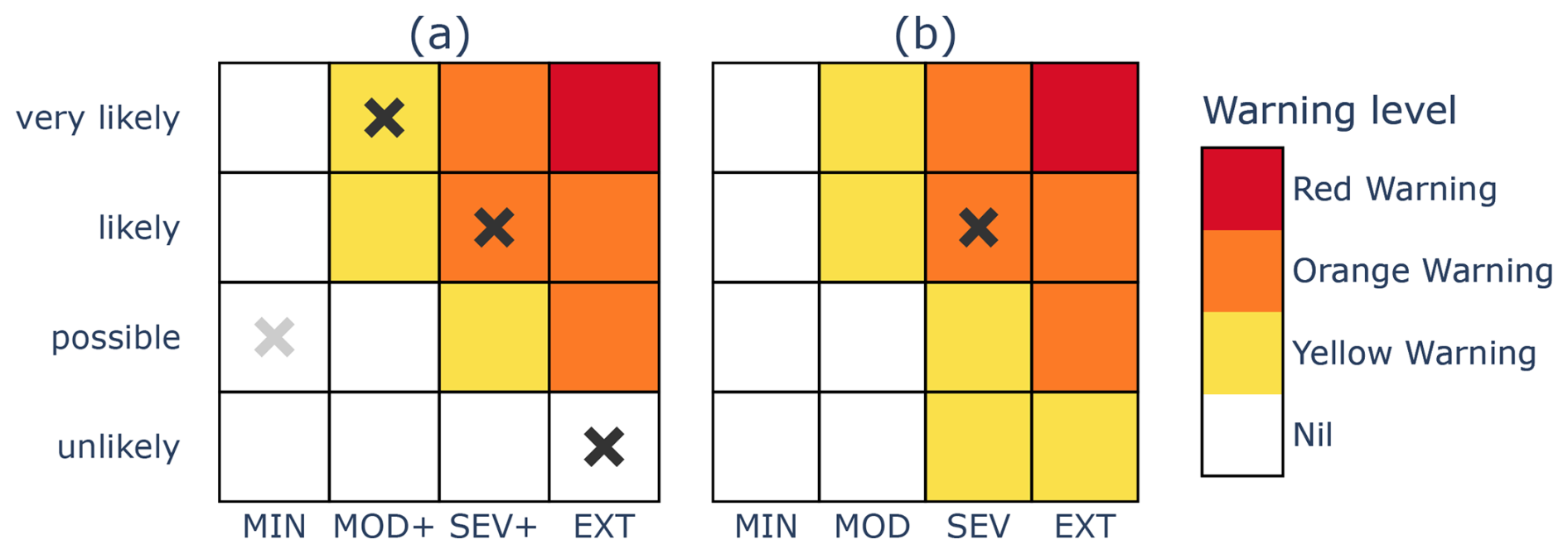
Figure 3 Two matrices demonstrating key structural differences between the framework outlined in Sect. 2.1, indicated by (a), and the approach used by the UKMO, indicated by (b).

There are three major structural differences between the UKMO warning framework, as presented in their risk matrix assessments, and the general framework detailed in Sect. 2.1. First, the UKMO matrix assigns a Yellow Warning level to some cells in the bottom row of their matrices, contravening property (a) for the warning scaling. The implication, if taken literally, would be a perpetual warning at the Yellow Warning level or higher because the risk of severe weather is at least unlikely. Indeed, Neal et al. (2014) define the lowest certainty category to be the set of probabilities less than 20 % and do not prescribe a lower bound above 0 % for this category.

The second difference is that when each of the severity categories of the UKMO matrices is labelled (e.g. Neal et al., 2014, Fig. 8), they appear to be a partition of the outcome space (akin to MIN, MOD, SEV and EXT) rather than a predominantly nested sequence of severity categories (MIN, MOD+, SEV+, EXT). To understand why we advocate for the nesting property, consider the following forecasts for the matrix of Fig. 2b but altered so that the severity categories are MIN, MOD, SEV and EXT:

• Forecast A. The forecast probability that the outcome is MOD, SEV and EXT is 9 %, 9 % and 9 % respectively. The resulting warning level is a Nil warning.

• Forecast B. The forecast probability that the outcome is MOD, SEV and EXT is 11 %, 0 % and 0 % respectively. The resulting warning level is a Yellow Warning.

We argue that Forecast A is more threatening: in Forecast A the probability that the outcome is MOD+ is 27 %, while in Forecast B the probability that the outcome is MOD+ is only 11 %. However, because the severity categories are MIN, MOD, SEV and EXT (rather than MIN, MOD+, SEV+ and EXT), Forecast A results in a lower warning level than Forecast B.

The third difference is that the framework presented here requires a certainty forecast for each of the nested severity categories (MOD+, SEV+, EXT) so that the full scope of potential threat is brought to bear on the final warning level issued. On the other hand, a forecast for each column is not a requirement for the warning service of the UKMO, as illustrated by the single tick in Fig. 1 and single cross in Fig. 3b.

Nonetheless, our framework and the UKMO warning service framework, as actually practised, may have fewer differences than mentioned above. For example, perpetual warnings are not a feature of their service because some small positive likelihood of a hazard is required to issue a warning, notwithstanding the presentation of their risk matrices. Similarly, the ensemble-based first-guess support tool for the warning service (MOGREPS-W) has a positive probability as its lower bound for generating a warning, as well as meteorological exceedance criteria for impact categories suggestive of the nesting property (Neal et al., 2014).

2.3 Warnings that vary with lead time

In many global alerting systems, the warning level is informed by the urgency of the hazard (Neußner, 2021), which typically depends on the time to onset. To accommodate this, warning scaling can be defined to vary with lead time if desired, allowing warning level to change as time to hazard onset reduces, even if the severity and certainty of the threat remain constant. This approach enables greater control of the communication and dissemination of information to the public, as discussed further in Sect. 5.

Figure 4 Examples of three scaling matrices and the trivial NIL STATE matrix.

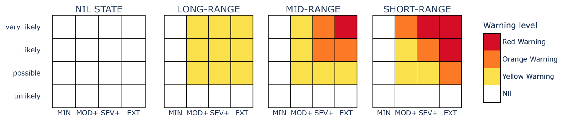
To incorporate lead time into warning level decisions, the composite warning scaling can be thought of as a series of risk matrix “phases” which apply during distinct time intervals in the warning period. This is illustrated in Fig. 4, which shows three sequential matrices applying at “LONG-RANGE”, “MID-RANGE” and “SHORT-RANGE”, in addition to the trivial “NIL STATE” matrix. In this example, for a given position in the matrix, warning level is non-decreasing with reducing lead time. That is, for any constant severity–certainty pair, the warning level remains constant or increases as the hazard becomes more imminent. In all cases, the longest lead time phase is the trivial NIL STATE matrix in which the lowest warning level is applied for all severity and certainty couples. Any standard two-dimensional warning scaling can be viewed as a special case of this approach with two lead time phases: the shorter lead time phase consists of the specified scaling matrix, and the longer lead time phase corresponds to the NIL STATE matrix.

2.4 Mathematical description of the general framework

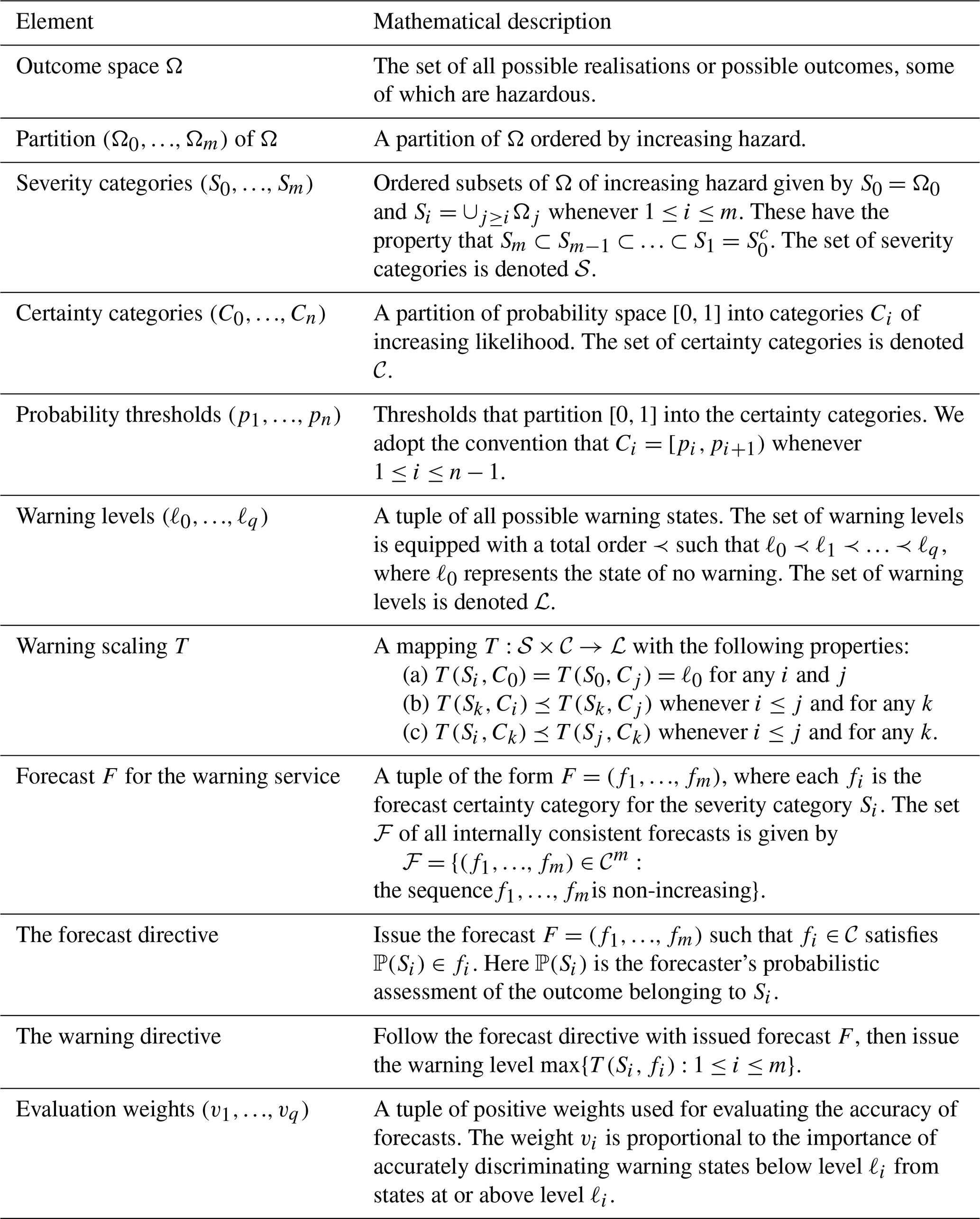
Each of the elements of the warning framework described in Sect. 2.1 has a corresponding mathematical description, presented in Table 1. Readers who prefer to avoid mathematical details may skip ahead to Sect. 3. For readers who would like to understand how risk matrix forecasts and the warnings generated by them can be evaluated using consistent scoring functions, the most important aspect of Table 1 is the following notation: for appropriate index i, each severity category is denoted by S_i, each certainty category by C_i, each probability threshold by p_i and each warning level by ℓ_i.

Table 1 A mathematical description of the elements of the warning framework. The integers m, n and q are positive. Evaluation weights, the final entry of the table, are discussed in Sect. 3.

An interval of the real numbers ℝ with endpoints a and b is denoted by [a,b] if both endpoints are included in the interval, [a,b) if only a is included and (a,b) if both endpoints are excluded. The convention that the left endpoint of C_i is included but not the right endpoint, as per $C_i=[p_i,p_{i+\mathrm{1}})$, can be changed, with appropriate modification to the scoring functions introduced in Sect. 3.

To illustrate some of the notation of Table 1, examples (E1) and (E2) of Sect. 2.1 can be stated as follows.

• (E1)

  This warning service for hazardous temperatures has outcome space $\mathrm{\Omega }=(-\mathrm{273.15},\mathrm{\infty })$ in units of degrees Celsius. Its severity categories are defined by $S_{\mathrm{0}}=[\mathrm{0},\mathrm{35}]$, $S_{\mathrm{1}}=(-\mathrm{273.15},\mathrm{0})\cup (\mathrm{35},\mathrm{\infty })$, $S_{\mathrm{2}}=(-\mathrm{273.15},-\mathrm{5})\cup (\mathrm{40},\mathrm{\infty })$ and $S_{\mathrm{3}}=(-\mathrm{273.15},-\mathrm{10})\cup (\mathrm{45},\mathrm{\infty })$.

• (E2)

  This warning service for hazardous hailstones and wind gusts has outcome space $\mathrm{\Omega }=[\mathrm{0},\mathrm{\infty })\times [\mathrm{0},\mathrm{\infty })$, where a possible outcome (h,g) in Ω is a combination of the maximum hailstone diameter h in millimetres and the maximum wind gust g in metres per second. Its severity categories are defined by $S_{\mathrm{0}}=[\mathrm{0},\mathrm{20})\times [\mathrm{0},\mathrm{25})$, $S_{\mathrm{1}}=[\mathrm{20},\mathrm{\infty })\times [\mathrm{25},\mathrm{\infty })$ and $S_{\mathrm{2}}=[\mathrm{50},\mathrm{\infty })\times [\mathrm{35},\mathrm{\infty })$.

If the matrix scaling also depends on lead time, then warning phase is an additional element required in the framework. In this case, the warning scaling T is also a function of warning phase, with the additional property that the warning level does not decrease with decreasing lead time, all else being equal.

3 Consistent scoring of warnings to evaluate warning systems

It is important to know how well competing forecasters or forecast procedures perform when generating warning products based on risk matrices. For example, one may want to know whether an upgrade to a forecast system produces more accurate warnings or whether the current method of producing warnings performs better than not issuing a warning at all (i.e. always issuing a Nil warning level).

In this section, we present a new scoring function, called the risk matrix score, which enables such questions to be answered. The risk matrix score gives a measure of forecast error, expressed as a number, for a particular forecast case when compared to the corresponding observation. The smaller the score, the better the forecast. A perfect score is 0. Forecasters or forecasting procedures can be compared by calculating the mean risk matrix score over many forecast cases, with a smaller mean risk matrix score indicating better predictive performance on average. The risk matrix score is also a consistent scoring function, which means that a forecaster's expected score will be minimised (i.e. optimised) by following the forecast directive. This property implies that the risk matrix score gives lower (i.e. better) scores to forecasters who make accurate probabilistic assessments and follow the forecast directive.

We also introduce a special case of the risk matrix score, called the warning score, which assesses the predictive accuracy of the final warning level. It does this by measuring forecast error only for the decision points in the risk matrix that are relevant to warning level determination. To calculate the warning score, the warning service must specify the relative importance of each warning level decision point. This specification is called the evaluation weights.

The main ideas are introduced, in a non-technical manner, in Sect. 3.1 using the example of a flood warning service. The risk matrix score and warning score are properly defined in Sect. 3.2 and 3.3. In Sect. 3.4 we present a synthetic experiment involving six fictitious forecasters who have access to different information (which affects the accuracy of their probabilistic assessments) and have different strategies when filling out the risk matrix (such as following the warning directive, over-warning or under-warning). The synthetic experiment illustrates desirable properties of the risk matrix score and warning score. Both scores correctly rank (a) forecasters who follow the directive but who differ in the accuracy of their probabilistic assessments and (b) forecasters who have identical probabilistic assessments but who differ in the degree to which they follow the forecast directive.

The risk matrix score (and by implication, the warning score) has a Python implementation in the open source scores package (Leeuwenburg et al., 2024). The scores documentation also includes a tutorial for how to use this implementation.

3.1 Introduction to scoring methods and evaluation weights

The basic ideas of warning service design and consistent scoring methods are illustrated using a flood warning service for a fictitious town situated on a river. The severity categories MOD+, SEV+ and EXT are defined using river height exceedance thresholds of 3, 4 and 6 m respectively.

When the river height exceeds 3 m (MOD+), the low-level causeway is flooded, leading to lengthy detours and traffic bottlenecks around the high-level bridge. Consultation with community members in the town suggests that a miss (i.e. forecast under 3 m but observation over 3 m) causes similar problems to a false alarm (i.e. forecast over 3 m but observation under 3 m). This means that the optimal probability threshold for warning for the MOD+ category is 50 %.¹

When the river height exceeds 4 m (SEV+), low-lying areas of the town are inundated, resulting in the closure of the primary school. Community consultation suggests that a miss (i.e. forecast under 4 m but observation over 4 m) is about 3 times worse than a false alarm (i.e. forecast over 4 m but observation under 4 m). This means that the optimal probability threshold for warning for the SEV+ category is 25 %.

When the river height exceeds 6 m (EXT), a river levee is breached, and significant inundation occurs, resulting in a third of the town becoming isolated by floodwaters. Community consultation suggests that a miss (i.e. forecast under 6 m but observation over 6 m) is about 4 times worse than a false alarm (i.e. forecast over 6 m but observation under 6 m). This means that the optimal probability threshold for warning for the EXT category is 20 %.

A Yellow Warning is warranted if the risk of exceeding the MOD+ threshold of 3 m is at least 50 %. An Orange Warning is warranted if the risk of exceeding the SEV+ threshold of 4 m is at least 25 %. A Red Warning is warranted if the risk of exceeding the EXT threshold of 6 m is at least 25 %. The warning level issued (if not Nil) is the highest such level. This flood warning service can be represented by the risk matrix depicted in Fig. 5.

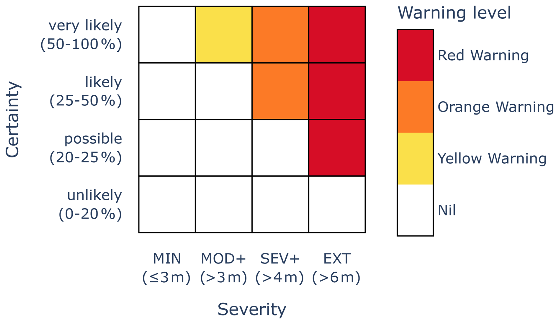
Figure 5 Risk matrix for a flood warning service, with severity categories defined based on river height.

We now discuss how forecasts for this warning service are scored in a manner that is consistent for this warning service. To follow the forecast directive, the forecaster must select one cell (i.e. certainty category) for each of the MOD+, SEV+ and EXT columns in the risk matrix. For each column, there are three probability decision points corresponding to the probability thresholds 20 %, 25 % and 50 %. In total, there are nine decision points (three probability thresholds for each of the three columns). For example, for the (EXT, 20 %) decision point, the forecaster must decide whether the likelihood of an EXT outcome is less than 20 % or at least 20 %.

To construct the risk matrix score, we first score, in a consistent manner, the forecast for each of the nine decision points. Consistency here means that the scores for a miss and a false alarm are appropriate for the particular probability threshold. For example, the following scores apply to the (EXT, 20 %) decision point:

• a false alarm (forecast is at least 20 %, and EXT is not observed) is given a score of 0.2

• a miss (forecast is less than 20 %, and EXT is observed) is given a score of 0.8

• a hit (forecast is at least 20 %, and EXT is observed) is given a score of 0

• a correct negative (forecast is less than 20 %, and EXT is not observed) is given a score of 0.

Note that scores are oriented so that a lower score implies a better forecast. For the (EXT, 20 %) decision point, a miss is penalised 4 times more than a false alarm, which is consistent with community consultation. The score for a false alarm is equal to the probability threshold for this decision point (i.e. 20 % or 0.2), while the score for a miss is equal to the complementary probability (i.e. 80 % or 0.8). Hits and correct negative receive a perfect score of 0.

The risk matrix score is then a weighted sum of all the scores for each of the nine decision points. If all decision points were of equal importance for the warning service, it would be appropriate to apply a weight of 1 for each of the nine decision points. In general, weights should be non-negative, and if we were to assess how forecasters fill out the risk matrix (without regard to warning scaling or warning level), then we should take positive weights for each decision point.

However, for this flood warning service, not every decision point is equally important. In fact, for determining the final warning level, there are exactly three relevant decision points: (MOD+, 50 %), (SEV+, 25 %), and (EXT, 20 %). That is, to determine the final warning level, we only need to know whether the forecaster forecasted above or below each of those decision points. If the accuracy of the final warning level is all that matters, then we put positive weights on the scores for those three decision points and assign a weight of 0 for the remaining six decision points.

This segues into the concept of evaluation weights. Evaluation weights quantify the importance of accurately discriminating between each of the warning levels. For this flood warning service, the Nil warning versus Yellow Warning decision point is the least important. The costs of preemptively erecting detour signs at the low-level causeway if the river stays below 3 m or of belatedly reacting to the situation after the causeway has flooded are low compared to the corresponding costs at the Yellow Warning versus Orange Warning decision point. At the Yellow–Orange Warning level decision point, an incorrect forecast results in either unnecessary preemptive school closures or reactive school closures. At the Orange Warning versus Red Warning decision point, the stakes of an incorrect warning decision are even higher, resulting in either unnecessary evacuations or stranded communities. Community consultation suggests that the relative importance of the Nil–Yellow, Yellow–Orange and Orange–Red Warning level decision points is in the ratio $\mathrm{1}:\mathrm{3}:\mathrm{10}$. We say that the evaluation weights for this flood warning service are (1, 3, 10).

This gives rise to the warning score, which is a special case of the risk matrix score but with weights in the weighted sum determined by the warning scaling and evaluation weights (see Sect. 3.3 for details). For the flood warning service, this means that the warning score is the weighted sum of the scores for each of the decision points in the risk matrix, where the weight on the (MOD+, 50 %) decision point is 1, the weight on the (SEV+, 25 %) decision point is 3, the weight on the (EXT, 20 %) decision point is 10 and the weight on the six remaining decision points is 0.

Evaluation weights should be given to forecasters in advance of them issuing warnings. The weights indicate the relative importance of each decision point and indicates how forecasters should allocate resources, given time and information constraints, to make the best possible warning decisions. Although the process for determining weights in this fictitious flood example was presented straightforwardly, this framework motivates further research into developing best practices for eliciting thresholds and weights through stakeholder consultation.

3.2 The risk matrix score

In this section we give a mathematical definition of the risk matrix score and advocate its usage from the perspective of decision theory.

There are many different scoring functions that could be used for evaluating forecasts for risk matrices but not all reward desirable or penalise unwanted forecasting behaviour. Powerful arguments have been presented (Murphy and Daan, 1985; Engelberg et al., 2009; Gneiting, 2011) that when the requested forecast is not in the form of a full probability distribution, either the scoring function should be made known to the forecaster ahead of time or a “forecast directive” should be given to the forecaster for how to convert their probability distribution to a forecast in the requested form. In the second case, the scoring function should be consistent with the forecast directive, which essentially means that the forecaster's expected score will be optimised by following the forecast directive.

We agree with this perspective. In our case, the forecast directive has been specified (see Sect. 2.1 and Table 1), so in the following we construct a family of scoring functions that are consistent with the forecast directive. See Appendix A for a precise mathematical definition of consistency in this context. As illustrated in Sect. 3.4, using a consistent scoring function provides the following benefits: (i) it rewards forecasters who make accurate probability assessments and follow the forecast directive, (ii) it penalises forecasters who follow the forecast directive but use poorer probabilistic assessments, and (iii) it penalises forecasters who make accurate probabilistic assessments but do not follow the forecast directive (Holzmann and Eulert, 2014).

We begin by using so-called elementary scoring functions (Ehm et al., 2016) to score the forecast relative to each decision point in the risk matrix. Using the notation of Table 1, the elementary scoring function ES_i,j, associated with severity category S_i and probability threshold p_j, is given by

$$\begin{array}{}\text{(1)}& {\mathrm{ES}}_{i,j}(F,y)=\left\{\begin{array}{ll}{p}_j,& y\notin S_i\text{and}{f}_i\text{lies on or above}{p}_j\\ \mathrm{1}-p_j,& y\in S_i\text{and}{f}_i\text{lies below}{p}_j\\ \mathrm{0},& \text{otherwise},\end{array}\right.\end{array}$$

where $F=(f_{\mathrm{1}},\mathrm{\dots },f_m)$ is the forecast for the warning service, f_i is the corresponding forecast for the severity category S_i and y is the observation in the outcome space Ω. In other words, ES_i,j gives a score for forecasts relative to the (S_i,p_j) decision point in the risk matrix, giving a penalty of p_j for a false alarm, a penalty of 1−p_j for a miss and a perfect score of 0 otherwise.

The risk matrix scoring function, RMaS, is defined by

$$\begin{array}{}\text{(2)}& \mathrm{RMaS}(F,y)=\sum _{i=\mathrm{1}}^m\sum _{j=\mathrm{1}}^n{w}_{i,j}{\mathrm{ES}}_{i,j}(F,y),\end{array}$$

where F is the forecast for the warning service, y is the observation in the outcome space Ω and each w_i,j is a pre-specified non-negative weight with at least one such weight being strictly positive. In other words, the risk matrix score is a weighted sum of the forecast errors associated with each of the decision points (S_i,p_j) of the risk matrix. The weight w_i,j indicates the importance of issuing a forecast on the same side as the observation relative to the (S_i,p_j) decision point; failure to do so results in penalties for misses and false alarms amplified by a factor of w_i,j. Hence, the choice of weights should reflect which decision points are most important for the warning service. If all decision points have equal importance, then each weight could be assigned a value of 1. From the forecaster's perspective, the choice of weights guides the focus for improvements in forecast system development.

The proof that the risk matrix score is consistent with the forecast directive is given in Appendix A. In essence, it is shown that each elementary scoring function is consistent and that consistency is preserved through weighted sums of consistent scoring functions. The choice of non-negative weights does not affect the score's consistency with the forecast directive, nor does it affect the optimal conversion rule from a forecaster's full probability distribution to the forecast for the warning service. However, the weights do indicate which decision points may require more attention when fine-tuning forecasting procedures.

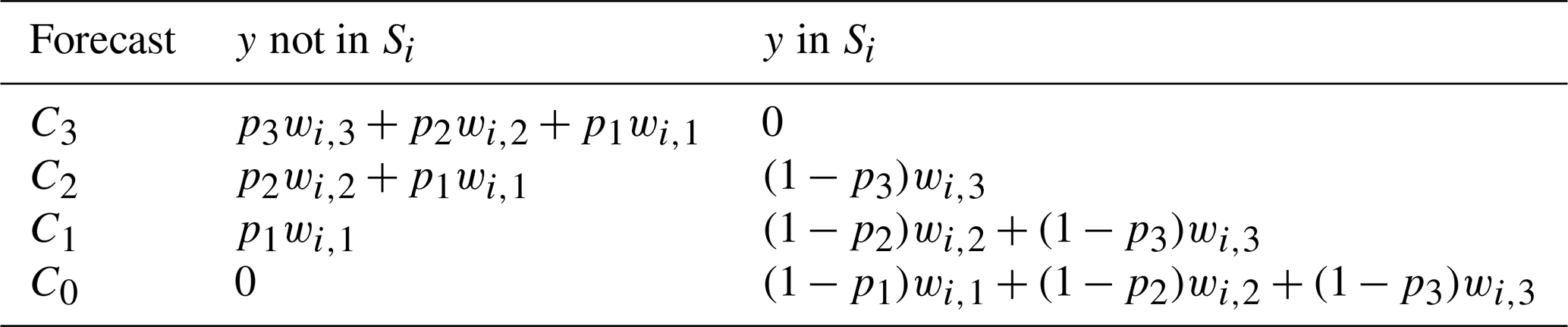
The risk matrix score can be decomposed as a sum of contributing scores for the forecast for each column of the risk matrix, excluding the leftmost column. That is, $\mathrm{RMaS}(F,y)={\sum }_{i=\mathrm{1}}^m{\mathrm{CS}}_i(F,y)$, where ${\mathrm{CS}}_i(F,y)={\sum }_{j=\mathrm{1}}^n{\mathrm{ES}}_{i,j}(F,y)$. We call CS_i(F,y) the column score associated with severity category S_i. The column score for S_i is presented in tabular form in Table 2 for the case when n=3 (i.e. there are three probability thresholds). Note that a perfect column score of 0 is achieved when the lowest certainty category C₀ was forecast and the observation y was not in S_i or when the highest certainty category C₃ was forecast and the observation y was in S_i.

Table 2 The column score associated with severity category S_i is given by the entries in the table for the case where there are four certainty categories from C₀ to C₃. The score depends on whether the observation y belongs to S_i and which certainty category was forecast.

A tabular form of the risk matrix score is a concatenation of tables of column scores. Table 3 illustrates this for the Sydney rainfall example (Fig. 2b), where we have set each weight w_i,j to be 1. Note that, on average, false alarms (non-zero scores in the left column of each severity category) are penalised less than misses (non-zero scores in the right column of each severity category). This is because the probability thresholds are on average closer to 0 than to 1.

Table 3 Components of the risk matrix score in tabular form for the Sydney rainfall example, where each of the weights w_i,j is 1.

We now calculate the risk matrix score for the forecast in the Sydney rainfall example (Fig. 2b), again assuming that each of the weights w_i,j is 1. The observed rainfall was 136 mm, which belongs to MOD+ but not to SEV+ and EXT. The MOD+ forecast was “likely”, so the column score for the MOD+ category is 0.3. The SEV+ and EXT forecasts were both “possible”, so the column scores for SEV+ and EXT are both 0.1. The risk matrix score is the sum of these contributions, namely 0.5. Had another forecaster failed to issue a warning by forecasting “unlikely” for MOD+, SEV+ and EXT, they would have received a risk matrix score of 1.8. With this choice of weights, the second forecaster performed worse than the first forecaster because they received a higher risk matrix score.

The risk matrix score is an extension of two special cases of the FIRM score. The risk matrix score with exactly two certainty categories reduces to one case of the FIRM score (Taggart et al., 2022, Sect. 4.1), while the risk matrix score with exactly two severity categories reduces to another case of the FIRM score (Taggart et al., 2022, Sect. 5.4). Moreover, our risk matrix warning framework and accompanying risk matrix score can also handle situations beyond the FIRM framework. This includes warning services with levels whose probability thresholds decrease with increasing severity (e.g. Fig. 5), thereby providing a coherent solution to problems discussed by Taggart et al. (2022, Appendix E). On the other hand, the FIRM framework provides a decision-theoretically coherent framework for (a) reducing the penalties applied to near misses and close false alarms and (b) warnings based on expected value forecasts. Incorporating these features into a generalisation of the risk matrix score is one avenue for future research.

Finally, although not formally proved in this article, the characterisation of consistent scoring functions for the expectation functional (Savage, 1971; Gneiting, 2011; Ehm et al., 2016), applied to the context of binary outcomes, essentially implies that any scoring function that is consistent with the forecast directive is in the form of the risk matrix score. Measures of risk that are not of this form (e.g. the product of certainty and severity) will be inconsistent with the forecast directive and hence with decision-theoretic coherent use of risk matrices. Although not expressed in these terms, this is the essence of a major criticism of the conventional use of risk matrices in risk management (Cox, 2008). Our framework is suitable for any area of risk management, provided that the risk matrix itself represents an adequate model of risk for the application.

3.3 The warning score

The warning score WS is a special case of the risk matrix score RMaS, where the weights w_i,j are selected to assess predictive performance only for the decision points (S_i,p_j) in the risk matrix that potentially lead to a change in the final warning level. Decision points (S_i,p_j) that are irrelevant for warning level determination have corresponding weights w_i,j set to 0. The classification of a weight being either 0 or positive is determined by the warning scaling. The value of each positive weight is determined by pre-specified evaluation weights, as detailed below.

To appreciate the classification of weights as a function of warning scaling, consider the LONG-RANGE scaling of Fig. 4 as a simple example. In the MOD+ column, the only important decision point, as far as warning level is concerned, is the p₁ probability threshold (that is, the threshold between “unlikely” and “possible”) because a change in warning level occurs at that threshold. A forecaster only needs to decide whether MOD+ is (a) “unlikely” or (b) “possible” or higher to determine the forecast warning level for the column. Moreover, because of the nesting property for severity categories, the forecast relative to the (MOD+, p₁) decision point completely determines the warning level. Hence, the weights for the warning score WS for the LONG-RANGE scaling are all 0, except for the positive weight w_1,1, which corresponds to the sole decision point (MOD+, p₁) that determines the final warning level.

Recall from Table 1 that (${\mathrm{\ell }}_{\mathrm{0}},\mathrm{\dots },{\mathrm{\ell }}_q$) is the tuple of all possible warning levels. To determine the choice of values for the positive weights in the warning score, we introduce corresponding warning evaluation weights ($v_{\mathrm{1}},\mathrm{\dots },v_q$). Each weight v_i is a positive number that is proportional to the importance of accurately discriminating warning states below the level ℓ_i from warning states at or above the level ℓ_i. See the flood warning service of Sect. 3.1 for an example of how evaluation weights might be determined.

Figure 6 Illustration of the algorithm for weight selection using the ZETA scaling.

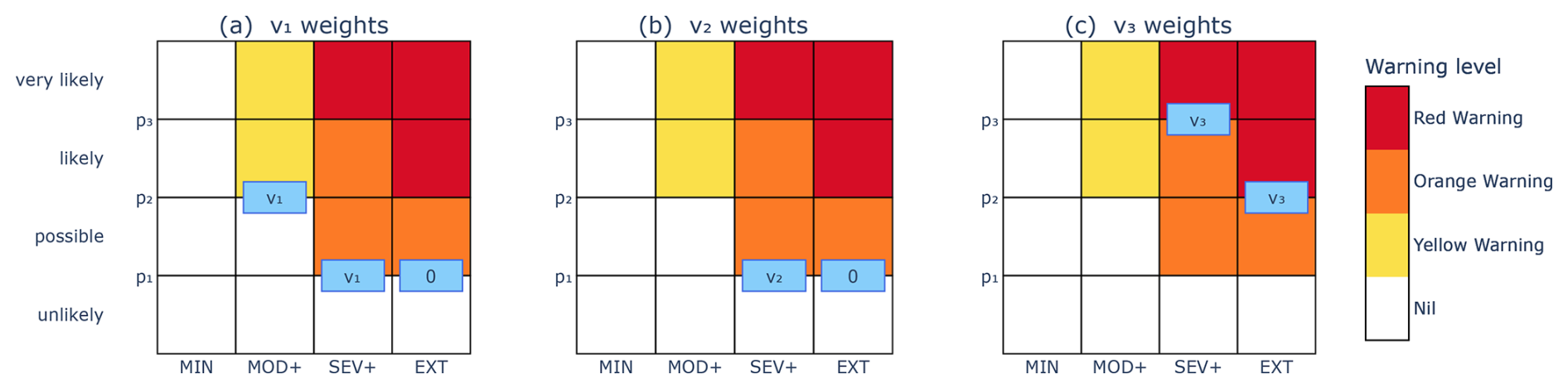
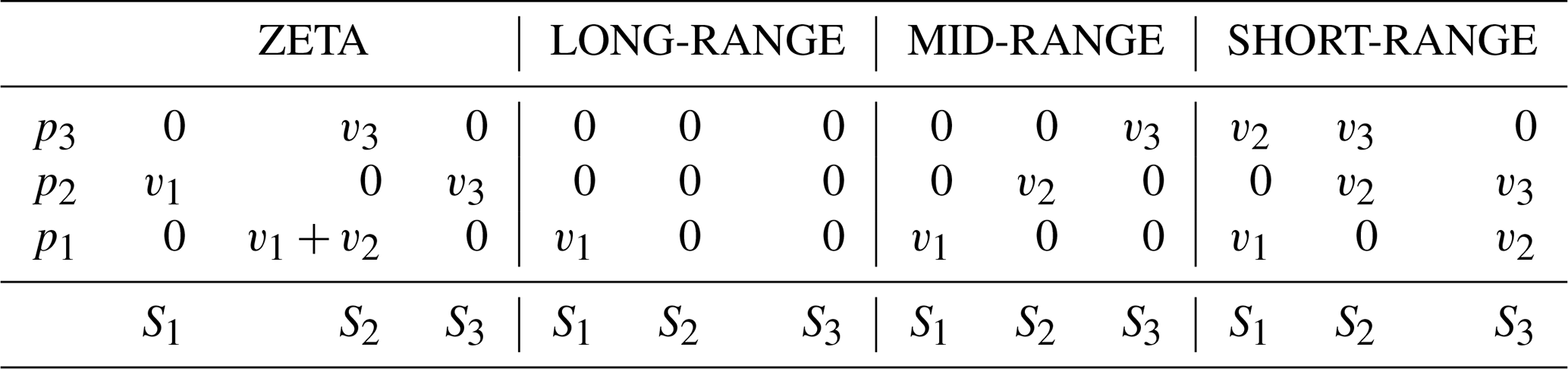
Given a warning scaling and evaluation weights ($v_{\mathrm{1}},\mathrm{\dots },v_q$), the weights w_i,j for the corresponding warning score WS can be determined by an algorithm that identifies which decision points are critical for determining the final warning level. The algorithm is stated and justified in general terms in Appendix B. Here we illustrate the algorithm using evaluation weights ($v_{\mathrm{1}},v_{\mathrm{2}},v_{\mathrm{3}}$) and the warning scaling of Fig. 6, which we call the ZETA scaling. The ZETA scaling illustrates all facets of the algorithm. We start with the first warning score weight v₁, which corresponds to the discrimination of Nil from Yellow Warning (or higher) levels. For each column, we identify any probability thresholds where the colour changes from white to yellow (or darker). These occur at the decision points (MOD+,p₂), (SEV+,p₁) and (EXT,p₁), as illustrated with the blue boxes in Fig. 6a. For each probability threshold p_i with a blue box, we assign a value of v₁ to the leftmost box and a value of 0 to any remaining boxes at the same probability level. In this case, the decision points (MOD+,p₂) and (SEV+,p₁) were assigned the value v₁, and the decision point (EXT,p₁) was assigned the value 0. We now repeat this process for v₂ by identifying probability thresholds where the colour changes from yellow (or lighter) to orange (or darker). The decision points are (SEV+,p₁) and (EXT,p₁). Both are at the same probability threshold, so we assign a value of v₂ to the leftmost box and 0 to the remaining boxes, as indicated in Fig. 6b. Repeating the process for v₃, the value v₃ is assigned to each of the decision points (SEV+,p₃) and (EXT,p₂), since these are the points where the colour changes from orange (or lighter) to red, as indicated in Fig. 6c. The final step of the process is to sum up all the values for each decision point, assigning a value of 0 to any remaining decision points without values. The set of weights for the ZETA scaling given by this algorithm is presented in Table 4, along with weights for the scalings of Fig. 4.

Table 4 Weights w_i,j associated with each (S_i,p_j) decision point for the ZETA, LONG-RANGE, MID-RANGE and SHORT-RANGE scalings when the evaluation weights $(v_{\mathrm{1}},v_{\mathrm{2}},v_{\mathrm{3}})$ are used. Here the severity categories are given by S₁=MOD+, S₂=SEV+ and S₃=EXT.

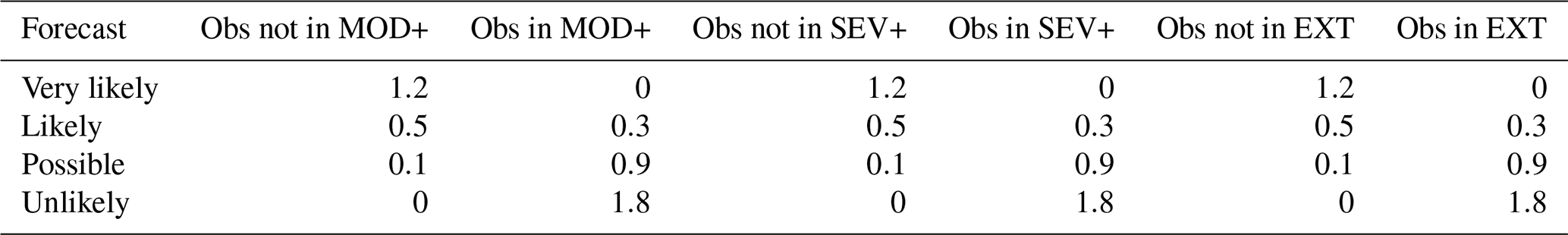
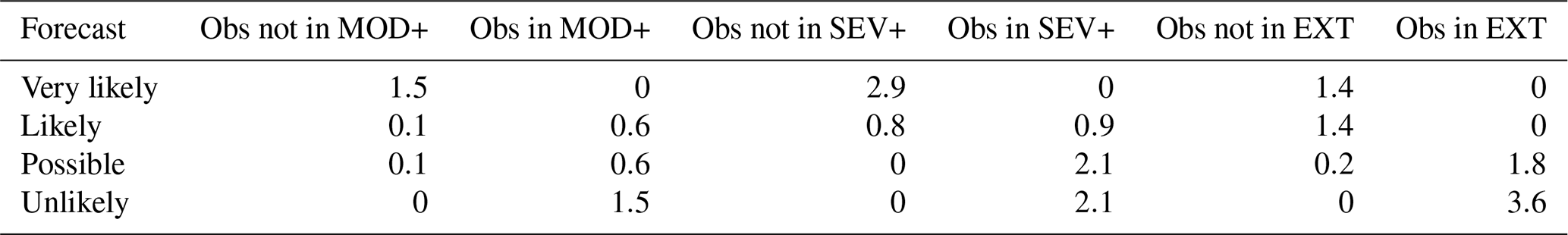
We calculate the warning score for the Sydney rainfall example (Fig. 2b) using illustrative evaluation weights $(v_{\mathrm{1}},v_{\mathrm{2}},v_{\mathrm{3}})=(\mathrm{1},\mathrm{2},\mathrm{3})$. In this case, the warning scaling is the SHORT-RANGE scaling, so the weights w_i,j for the warning score WS are given by the three rightmost columns of Table 4. Using these weights and the column score of Table 2, we obtain the warning score in tabulated form (Table 5). To score a particular forecast case, a column score for MOD+, SEV+ and EXT is obtained using Table 5, and the warning score is the sum of these. Recall that the observation was in MOD+ but not the other severity categories. The forecaster in the Sydney rainfall example obtained column scores of 0.6, 0 and 0.2 to obtain a final warning score of 0.8. A second forecaster, who forecasts “unlikely” for each severity category, receives a warning score of 1.5. Therefore, with this scaling and choice of evaluation weights, the first forecaster is again assessed as performing better. Note that the penalties in the MOD+ columns are the same for a forecast of “possible” or “likely”. This is because the scaling does not change (both cells are yellow in the matrix), and this is reflected in the scoring method.

Table 5 Components of the warning score WS in tabular form for the Sydney rainfall example (Fig. 2b), using evaluation weights (1, 2, 3).

3.4 Case study using synthetic forecasts

We now run a simple synthetic experiment to test whether the scoring methods described above are able to correctly rank competing forecasters who have varying levels of forecast capability and adherence to the forecast directive. We consider a simple warning service for hazardous outdoor heat, as depicted in Fig. 7, with certainty thresholds of 0.1, 0.3, and 0.5; severity thresholds for daily maximum temperature of 35, 37, and 40 °C; and warning scaling as shown.

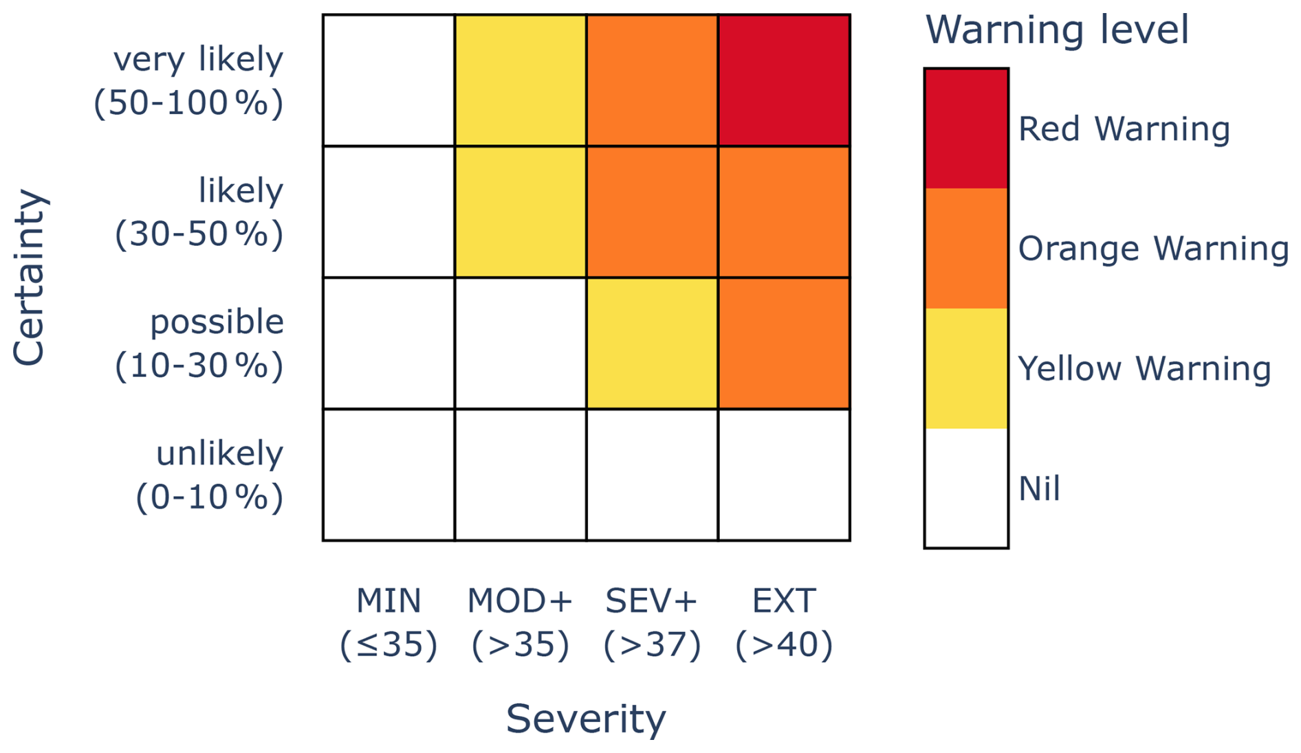
Figure 7 Risk matrix used for the synthetic experiment, warning for hazardous heat. The severity thresholds are for daily maximum temperatures in units of degrees Celsius.

Let 𝒩(μ,σ²) denote the normal distribution with mean μ and variance σ². Suppose that each observed daily maximum temperature y is generated from random variables y₁, y₂ and y₃ using the formula $y=y_{\mathrm{1}}+y_{\mathrm{2}}+y_{\mathrm{3}}$, where each random variable y_i is independent of the others, $y_{\mathrm{1}}\sim \mathcal{N}(\mathrm{20},{\mathrm{10}}^{\mathrm{2}})$, $y_{\mathrm{2}}\sim \mathcal{N}(\mathrm{0},{\mathrm{5}}^{\mathrm{2}})$ and $y_{\mathrm{3}}\sim \mathcal{N}(\mathrm{0},{\mathrm{2}}^{\mathrm{2}})$. The random variables y₁, y₂ and y₃ can be regarded as representing variability from seasonal, synoptic-scale and mesoscale weather processes respectively. The climatic distribution of maximum temperature is $\mathcal{N}(\mathrm{20},{\mathrm{10}}^{\mathrm{2}}+{\mathrm{5}}^{\mathrm{2}}+{\mathrm{2}}^{\mathrm{2}})$. The climatic probability of exceeding 35, 37 and 40 °C on any given randomly selected day is therefore 0.093, 0.067 and 0.039.

Six forecasters named NeverWarnNate, SeasonalSam, SynopticSally, RiskAverseRick, RiskTolerantReena and PlayfulPranay issue competing forecasts for this warning service. All six know the climatic distribution of maximum temperature.

• NeverWarnNate only knows about the climatic distribution. Using this distribution, he follows the forecast directive to issue categorical forecasts for the warning service. This means that his categorical forecasts for MOD+, SEV+ and EXT are always “unlikely” and that his warning level is always Nil.

• SeasonalSam has access to seasonal information y₁ but not synoptic or mesoscale information. She makes the ideal predictive distribution using this information, namely $\mathcal{N}(y_{\mathrm{1}},{\mathrm{5}}^{\mathrm{2}}+{\mathrm{2}}^{\mathrm{2}})$, and from this distribution follows the forecast directive to issue categorical forecasts for the warning service.

• SynopticSally has access to seasonal information y₁ and synoptic information y₂ but not mesoscale information. She makes the ideal predictive distribution using this information, namely $\mathcal{N}(y_{\mathrm{1}}+y_{\mathrm{2}},{\mathrm{2}}^{\mathrm{2}})$, and from this distribution follows the forecast directive to issue categorical forecasts for the warning service.

• RiskAverseRick has the same information as SynopticSally and makes the same ideal predictive distribution. However, he does not follow the forecast directive but instead converts his predictive distribution to categorical forecasts using lower certainty thresholds, namely 0.05, 0.2 and 0.4. Hence, he warns more frequently than SynopticSally.

• RiskTolerantReena has the same information as SynopticSally and makes the same ideal predictive distribution. However, she does not follow the forecast directive but instead converts her predictive distribution to categorical forecasts using higher certainty thresholds, namely 0.2, 0.4 and 0.6. Hence, she warns less frequently than SynopticSally.

• PlayfulPranay has the same information as SynopticSally and makes the same ideal predictive distribution. For each column, he identifies the warning level ℓ of the cell he would select to follow the forecast directive. If possible, he then selects an alternative cell with warning level ℓ, if such a cell exists; otherwise he follows the forecast directive. For example, if SynopticSally forecasts “likely” for SEV+, then PlayfulPranay forecasts “very likely”, and if SynopticSally forecasts “possible” for SEV+, so will PlayfulPranay. Hence, PlayfulPranay issues the same warning levels as SynopticSally but sometimes selects different certainty categories.

Based on this set-up, a good scoring function ought to rank SynopticSally ahead of SeasonalSam and SeasonalSam ahead of NeverWarnNate. All three forecasters make the best probabilistic predictions they can based on the information that is available to them, and all three follow the forecast directive. The difference between these three forecasters is that some have access to more information and can therefore make more accurate probabilistic predictions. Additionally, a good scoring function ought to rank SynopticSally ahead of RiskAverseRick and RiskTolerantReena. These three forecasters make identical probabilistic predictions of the risks. They differ because SynopticSally follows the forecast directive but RiskAverseRick and RiskTolerantReena do not. Finally, a good scoring function that takes into account every decision point in the matrix ought to rank SynopticSally ahead of PlayfulPranay, while a good scoring function that only takes into account decision points that affect warning levels should rank SynopticSally and PlayfulPranay equally.

Table 6 Mean risk matrix score $\stackrel{\mathrm{‾}}{\mathrm{RMaS}}$ and mean warning score $\stackrel{\mathrm{‾}}{\mathrm{WS}}$ for the synthetic experiment. A lower mean score is better.

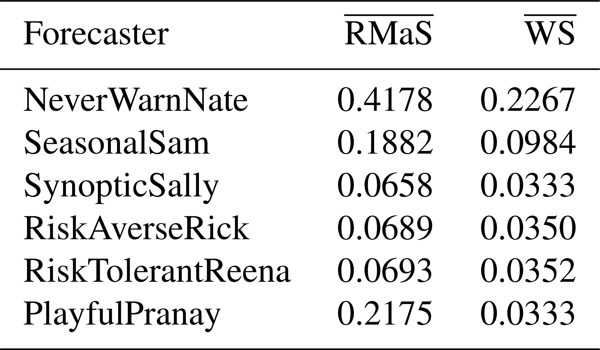
We now test the effectiveness of the risk matrix score and warning score at ranking these forecasters, where the weights for the risk matrix score RMaS and the evaluation weights are all 1. To conduct one synthetic experiment, the random variates y₁, y₂ and y₃ are generated; the probabilistic assessments of each forecaster are computed; and their issued categorical forecasts are then scored against the corresponding observation y. The experiment is repeated independently 1 million times, and the mean risk matrix score $\stackrel{\mathrm{‾}}{\mathrm{RMaS}}$ and the mean warning score $\stackrel{\mathrm{‾}}{\mathrm{WS}}$ are calculated for each forecaster. The results are given in Table 6. The results show that both mean scores meet the expectations of a good scoring function: SynopticSally has the lowest mean score, and SeasonalSam outperformed NeverWarnNate. The risk matrix score distinguished between SynopticSally and PlayfulPranay, while the warning score did not. Standard hypothesis tests for equipredictive performance (Gneiting and Katzfuss, 2014, Sect. 3.3) were conducted, and it was found that SynopticSally outperformed the other forecasters at the 5 % significance level, with the exception of PlayfulPranay with the warning score. Mean scores from RMaS are higher than those from WS because their respective sum of weights w_i,j is 9 and 5. Finally, even though RiskAverseRick and RiskTolerantReena do not follow the forecast directive, they still outperform SeasonalSam because the synoptic information they use gives them substantially more accurate and sharp probabilistic assessments.

4 Case study of warnings for heavy rainfall from Tropical Cyclone Jasper

We now illustrate the warning framework with a case study using operational ensemble precipitation forecasts for the northeastern parts of Queensland, Australia, which were impacted by Tropical Cyclone Jasper during mid-December 2023. The emphasis in this section is on how warning products can be generated and assessed given warning service specifications within the risk matrix framework rather than on how those specifications are determined.

4.1 Specifications for warning service and resultant warning products

To begin, we describe (without justification) a simple warning service for heavy rainfall for 17 December 2023.² The severity categories for the warning service are defined using climatological thresholds for heavy rainfall based on annual exceedance probabilities (AEPs) for a duration of 24 h at each location. The categories MOD+, SEV+ and EXT are defined by rainfall that exceeds 20 %, 10 % and 5 % AEPs respectively. The AEP values are taken from the 2016 Design Rainfall gridded dataset (Bureau of Meteorology, 2016; Johnson and Green, 2018) of the Australian Bureau of Meteorology (hereafter “the Bureau”). For example, for the city of Cairns,³ the thresholds for MOD+, SEV+ and EXT are 298, 357 and 415 mm.

The certainty categories for the warning service consist of probabilities p satisfying $\mathrm{0}\mathit{\%}\le p<\mathrm{10}\mathit{\%}$, $\mathrm{10}\mathit{\%}\le p<\mathrm{30}\mathit{\%}$, $\mathrm{30}\mathit{\%}\le p<\mathrm{50}\mathit{\%}$ and $\mathrm{50}\mathit{\%}\le p\le \mathrm{100}\mathit{\%}$, to which we assign the labels unlikely, possible, likely and very likely respectively.

The warning scaling depends on the issuance time of the warning relative to 17 December 2023, which is the validity period of the warning. All warnings are issued a couple of hours after midnight on the local day. Warnings issued early on the day of the validity period (a “day +0” lead time) use the short-range scaling (see Fig. 4). Warnings issued the day before (a “day +1” lead time) use the mid-range scaling. Warnings issued two days before the validity period (a “day +2” lead time) use the LONG-RANGE scaling.

We compare warnings based on forecasts from three different forecast systems: the 51-member ensemble prediction system from the European Centre for Medium-Range Weather Forecasts (ECMWF) (Molteni et al., 1996), the ECMWF's high-resolution numerical weather prediction model (hereafter called ECMWF deterministic) and the Bureau's operational 18-member ACCESS-GE3 ensemble prediction system (Bureau of Meteorology, 2019). The forecasts used from these systems have an initial condition time (or base time) of 12:00 UTC (a few hours before midnight local time). These forecasts could be used to issue warning products a couple of hours after midnight local time. Gridded AEP values and forecasts from each forecast system were regridded to a common grid prior to generating warning products.

We now explain how each of these forecast systems can be used to generate probabilities for each of the severity categories MOD+, SEV+ and EXT. In the simplest case, ECMWF deterministic forecasts a single value x (in millimetres) for 24 h rainfall at each location. This value is converted to a probability of 100 % if x falls within the severity category of interest or a probability of 0 % otherwise. For example, the day +0 ECMWF deterministic forecast for Cairns was 57 mm, which lies below the MOD+ threshold of 297 mm, and so we have $\mathbb{P}(\mathrm{MOD}+)=\mathrm{0}\mathit{\%}$.

The two ensemble prediction systems produce a single value x (in millimetres) for 24 h rainfall at each location for each ensemble member. The proportion of ensemble member values x that fall within the severity category of interest could be used as the probability forecast. To illustrate, we consider the day +0 ECMWF ensemble forecast for Cairns. Rainfall predictions from the 51 ensemble members are shown as 51 black crosses in Fig. 8, while the AEP thresholds are indicated using grey dotted vertical lines. For the EXT category, 6 out of 51 ensemble members exceeded the EXT threshold of 415 mm, so $\mathbb{P}\left(\mathrm{EXT}\right)=\mathrm{6}/\mathrm{51}\approx \mathrm{12}\mathit{\%}$, which falls into the “possible” category.

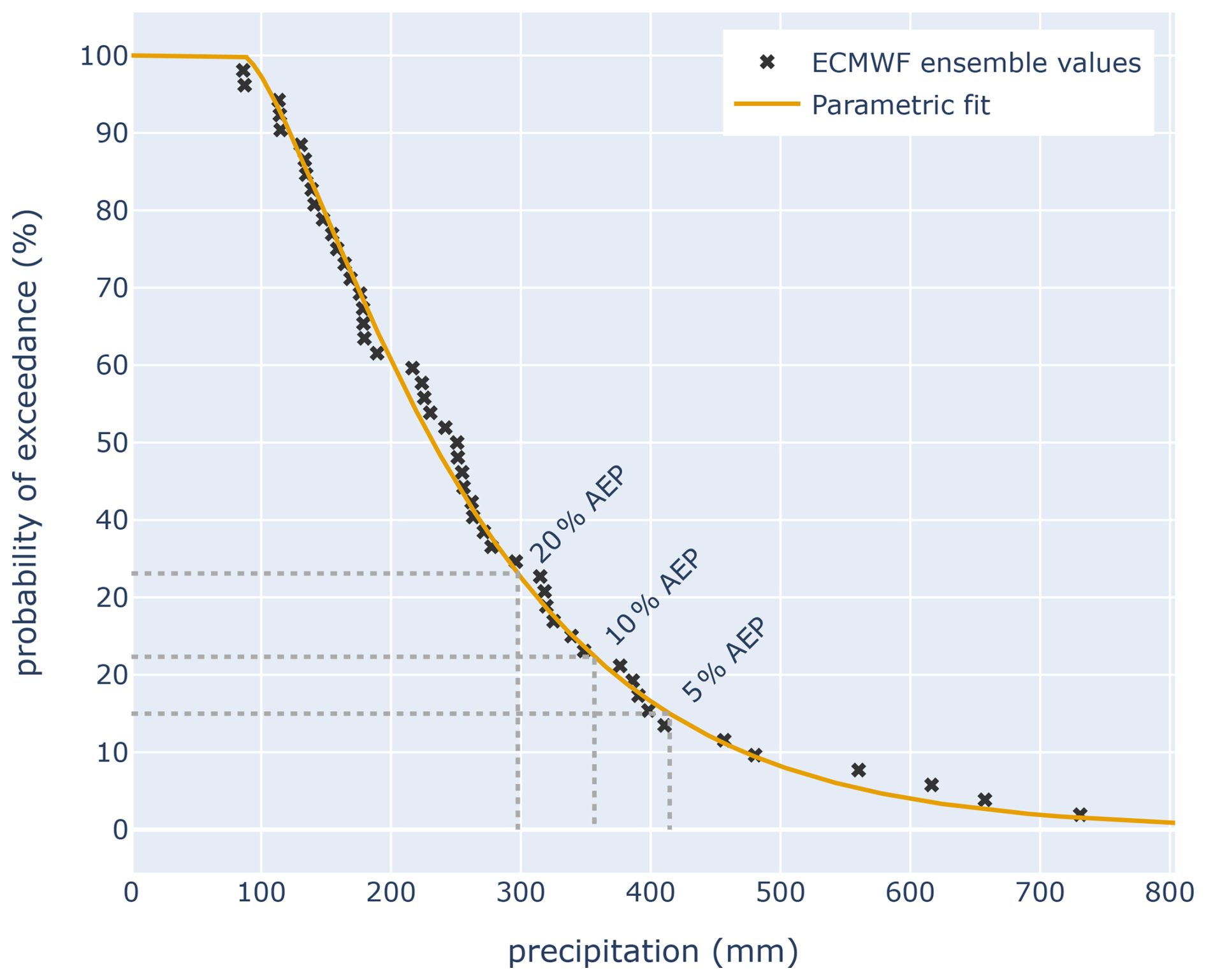
Figure 8 Probability of exceedance curve for daily precipitation on 17 December 2023 for Cairns, derived from the ECMWF ensemble forecast issued early on 17 December.

Rather than calculating ensemble probabilities using a simple proportion of members in the severity category, instead we fit the empirical ensemble distribution to a parametric distribution, as shown with the orange curve in Fig. 8. The fitting method is described in Appendix A of Taggart et al. (2025), drawing on the work of Balakrishnan and Wang (2000). In the Cairns example, the probability of exceeding 415 mm based on the parametric fit is 15 %, which also falls within the “possible” category. Fitting the data in this way gives the 18-member ACCESS-GE3 ensemble comparable resolution in probability space to the 51-member ECMWF ensemble and avoids the overinterpretation of forecast values from individual ensemble members, particularly for small ensembles.

With that set-up, we now generate warning products for heavy rainfall for 17 December 2023. Figure 9 shows warning sequences generated by the ECWMF ensemble (top row), ECMWF deterministic (middle row) and ACCESS-GE3 ensemble (bottom row), issued in the early hours of 15, 16 and 17 December (from left to right). The area of light blue shading indicates part of the Coral Sea, while the grey lines show boundaries of districts that are used by the Bureau's forecast and warning service. The warnings issued on 15 December (left column) only contain a Yellow Warning because LONG-RANGE warning scaling is used. The other issue dates (centre and right columns) contain a mix of Yellow, Orange and Red Warnings. Note that the ECMWF deterministic forecast can only ever produce “unlikely” or “very likely” forecasts, and so at day +0 it can never issue a Yellow Warning due to the SHORT-RANGE warning scaling. The ECMWF ensemble warning level in Cairns for day +0 is the Orange Warning, consistent with the PoE curve in Fig. 8.

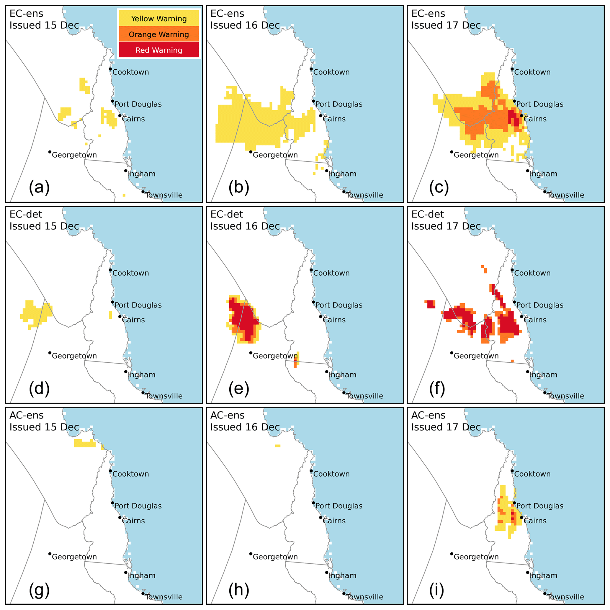
Figure 9 Warning sequences for 17 December 2023, as generated by the ECMWF ensemble (a–c), ECMWF deterministic (d–f) and ACCESS-GE3 ensemble (g–i). Issuance times are the early morning of each issue date. From left to right, the warning scaling used follows the LONG-RANGE, MID-RANGE and SHORT-RANGE matrices shown in Fig. 4.

4.2 Evaluation of the warning products

We now evaluate the predictive accuracy of the warning products. Precipitation accumulations for 17 December were observed over the domain of interest using a network of tipping-bucket rain gauges. After automated and manual quality assurance checks were conducted, 177 observations were obtained. Each observation was categorised as MIN, MOD, SEV and EXT according to warning service AEP thresholds (see Fig. 10). The observation for Cairns was 370 mm, which is categorised as SEV.

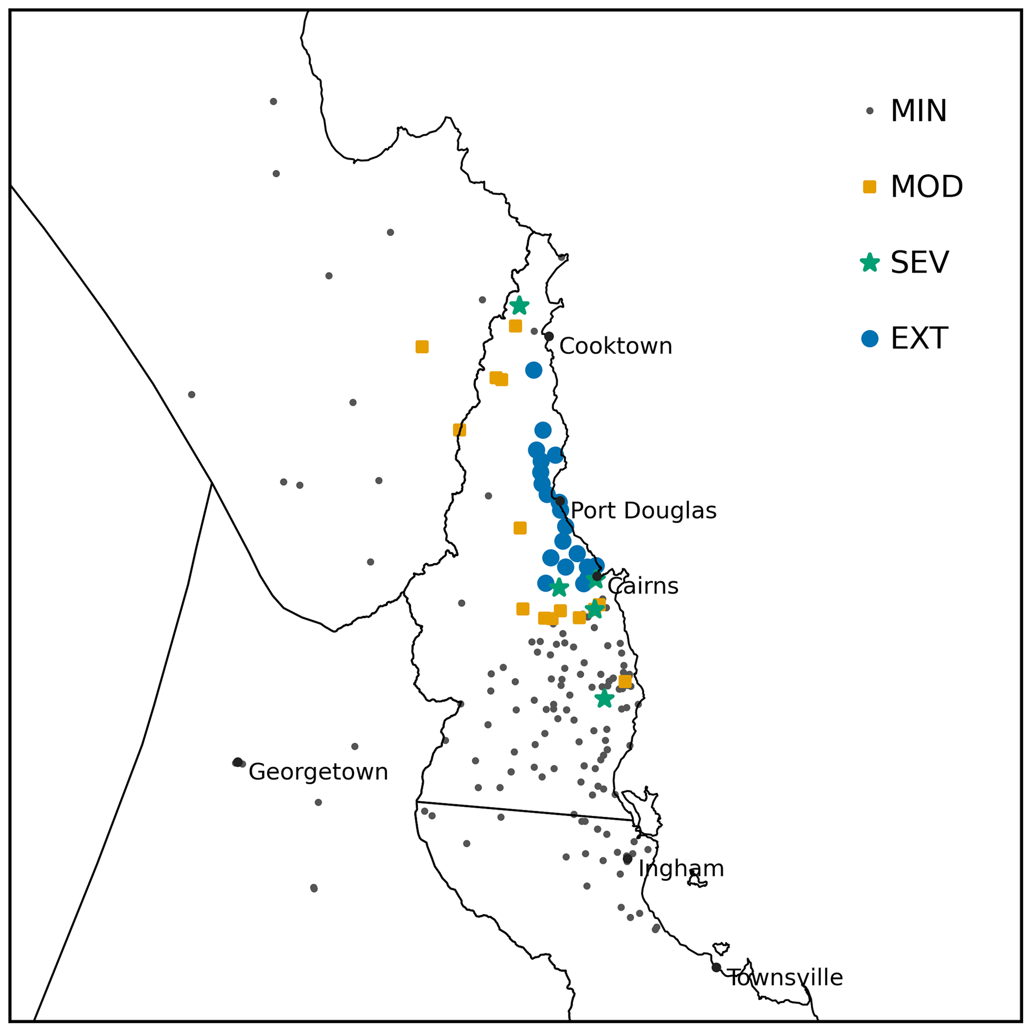
Figure 10 Observed 24 h precipitation for 17 December 2024, categorised by severity.

We begin with a subjective comparison of the warning products with the observations and then apply an objective evaluation using the risk matrix score and warning score. Observations in the EXT category were concentrated along the coast and adjacent hinterland between Cairns and Cooktown. MOD and SEV observations were recorded a little further inland and also a little to the south and north of the extreme observations. The remainder of the domain had observations in the MIN category. The warning products issued on 15 December generally did not produce a signal in the area of observed extreme rainfall, though there is signal inland of Cairns from the ECMWF ensemble. Both ECMWF warning products issued on 16 December have a signal for heavy rain inland to the north of Georgetown. There are very few rain gauges in this area, so whether this signal was accurate cannot be confirmed by data used in this study. Warnings issued early on 17 December all (correctly) have a signal inland of Cairns, while the warnings generated from the two ensembles also correctly include the coast between Cairns and Port Douglas. All three forecasts at all lead times mostly miss the heavy coastal rain observed between Port Douglas and Cooktown.

For an objective evaluation of the risk matrix forecasts, we use the risk matrix score with equal emphasis placed on each decision point in the risk matrix (i.e. a uniform weight scheme with $w_{i,j}=\mathrm{1}$). For an objective evaluation of the warning products, the warning score is used with evaluation weights (1, 1, 1) for their respective warning scalings. For each forecast system and issue time, forecasts are scored at each rain gauge, and the mean score across all rain gauges is then calculated. For comparison, we also calculate the mean scores for the strategy “never warn”. By taking an unweighted mean across all rain gauges, the mean score places a higher weight on predictive performance where the observation network is more dense. One possible justification for this is that rain gauges are generally located where impacts (due to the location of population, infrastructure or flood risk) are greater. If this emphasis is not desired, a weighted mean that places a higher weight on more isolated observations could be used.

The mean risk matrix scores by issue date, using the uniform weight scheme, are shown in Fig. 11a. A lower mean score is better. For each issue date, the ECMWF ensemble performed best. The ECMWF ensemble forecast also improved as the lead time decreased. In contrast, the ECMWF deterministic forecast did not improve with decreasing lead time because the heaviest rainfall shifted eastward from an area without observations to an area with many observations in the MIN category. Both ensemble forecasts performed substantially better than the never-warn strategy at lead day +0 (issue date of 17 December).

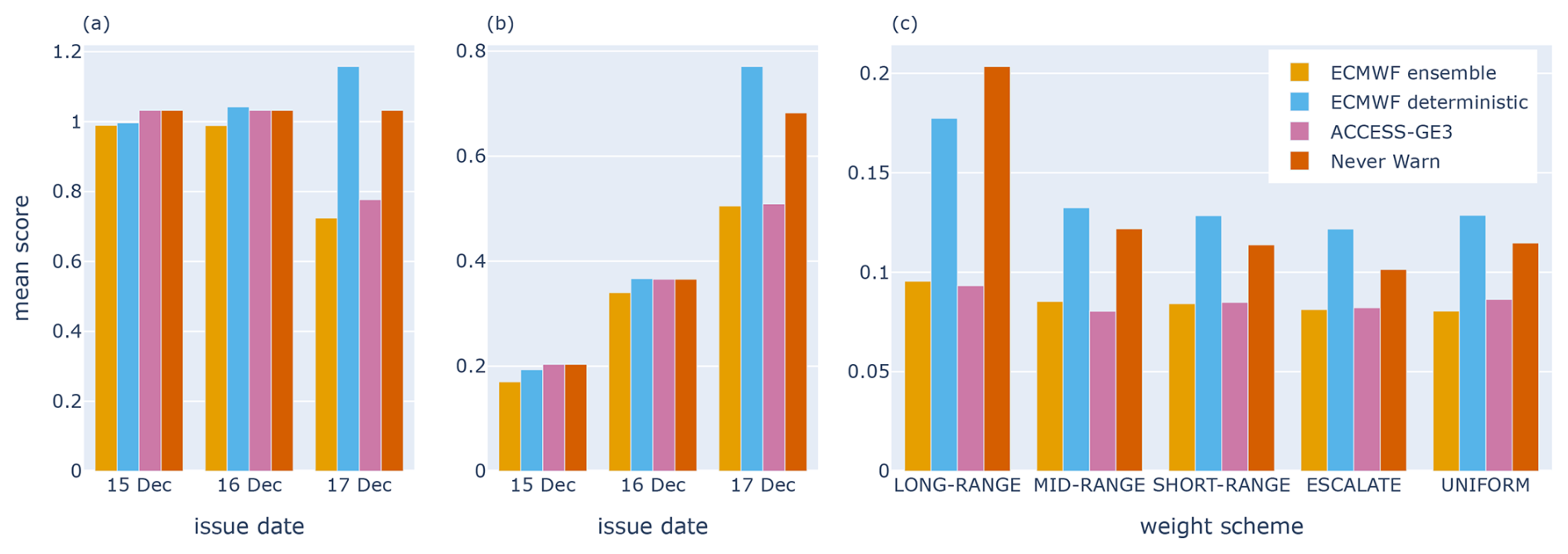
Figure 11 (a) Mean risk matrix scores $\stackrel{\mathrm{‾}}{\mathrm{RMaS}}$ for forecasts valid for 17 December 2023 by issue date, using a uniform weight scheme. (b) Mean warning scores $\stackrel{\mathrm{‾}}{\mathrm{WS}}$ for forecasts valid for 17 December 2023 by issue date. (c) Mean risk matrix scores $\stackrel{\mathrm{‾}}{\mathrm{RMaS}}$ for lead day +0 warnings valid for 17 December, each using a different weight scheme, with weights w_i,j normalised to sum to 1. In all graphs, a lower mean score is better.

The mean warning scores by issue date are shown in Fig. 11b. Once again, the ECMWF ensemble performed best on each issue date. The ACCESS-GE3 ensemble had the same score as the never-warn strategy at days +2 and +1, which is unsurprising given that its small warning footprint did not intersect with any rain gauges. ACCESS-GE3 outperformed the never-warn strategy at day +0 by warning for areas where MOD to EXT observations were observed near Cairns and Port Douglas. The ECMWF deterministic warning product issued on 17 December performed poorly, giving a confident warning signal over many rain gauges to the southwest of Cairns where precipitation did not exceed 20 % AEP. Note that the mean warning scores increase with decreasing lead time. This is because the warning scaling changes with lead time, and, consequently, the sum of the weights w_i,j used for scoring increases from 1 to 3 to 6 across lead days +2, +1 and +0.

Figure 11c shows the mean risk matrix scores for day +0 forecasts issued early on 17 December based on different weight schemes. The LONG-RANGE, MID-RANGE and SHORT-RANGE weight schemes are the same as those in Table 4, with $(v_{\mathrm{1}},v_{\mathrm{2}},v_{\mathrm{3}})=(\mathrm{1},\mathrm{1},\mathrm{1})$. The escalate weight scheme uses SHORT-RANGE scaling but with $(v_{\mathrm{1}},v_{\mathrm{2}},v_{\mathrm{3}})=(\mathrm{1},\mathrm{2},\mathrm{3})$. The uniform weight scheme uses the weights $w_{i,j}=\mathrm{1}$. For each weight scheme, weights are normalised to sum to 1 to allow for easier comparison between schemes. The results of Fig. 11c illustrate the general principle that forecaster rankings can depend on the choice of weight scheme (Ehm et al., 2016). For example, at day +0, ECMWF deterministic outperformed the never-warn strategy when assessed using the LONG-RANGE weight scheme but otherwise performed worse. Similarly, the ACCESS-GE3 ensemble had a lower mean score than the ECMWF ensemble using the LONG-RANGE scheme but not when using the uniform scheme.

We reiterate the importance of selecting weights prior to any evaluation of forecasts and ideally so that forecasters know them in advance. The selected weights should reflect warning service priorities and should not be manipulated to obtain desirable rankings of forecasters.

Finally, we emphasise that the Tropical Cycle Jasper case study is merely designed to illustrate the warning framework and its consistent scoring methods. A superior public weather warning service for heavy rainfall would warn for intense rainfall over varying durations (say 30 min to 48 h), and the period of intense rainfall could start at any time of day (not just at the start of the local day). A warning would be issued if the period of intense rainfall (irrespective of duration) overlapped with the warning validity period. Moreover, evaluation of competing forecasters would need to be conducted over a long period, accompanied by tests for statistical significance, to conduct statistical inference regarding whether any forecast system was superior.

5 Summary and discussion

We have presented a general framework for determining the warning level for a hazard based on a probabilistic forecast of the severity (or impact) of the hazard at a given warning lead time. The key tool used in the framework is the risk matrix, which gives a simple graphical representation of how a probabilistic forecast maps to a warning level and is thus a useful device both for those who issue warning levels and for those who wish to better understand or communicate them. While the use of risk matrices for the generation of warning levels is not new, a major contribution of this paper is to provide a structure for their use that is free of issues found in other frameworks. These include perpetual warnings, undesirable warning level de-escalations and warning level determinations based on incomplete risk assessments. We emphasise that the framework is hazard agnostic, could be used for multi-hazard warnings (e.g. combined rainfall and wind), and could be used when severity categories are replaced with well-defined impact or consequence categories with the appropriate structural properties. Some simpler warning frameworks, such as those with a one-to-one correspondence between warning level and severity category and where warning issuance is defined by a single fixed probability threshold (Taggart et al., 2022), are special cases of the general framework.

Another major contribution of this paper is to furnish the warning framework with accompanying evaluation tools that are consistent with the aims of such warnings. The risk matrix score can be used to assess the predictive accuracy of risk matrix assessments. The warning score, which is a special case of the risk matrix score, assesses the predictive accuracy of warning levels by assessing the accuracy of risk matrix forecasts at the decision points that are critical to warning level determination. Both scoring functions are consistent with the forecast directive to fill out the risk matrix assessment in line with warning service specifications. This means that forecasters who make good probabilistic assessments, given the information at hand, and who comply with the forecast directive will be rewarded, while poorer probabilistic assessments or non-compliance is penalised. The availability of consistent scoring functions allows the possibility of a cycle of continuous improvement in warning accuracy through forecast system upgrades that are objectively measured to be better than those of their predecessors. Over the long term, these scores, or skill score versions of them (Potts, 2003, p. 27), can also be used as key performance indicator measures for warning accuracy.

To establish a warning service based on our framework, several considerations must be addressed. Firstly, severity and certainty categories should be defined to reflect the intention of the warning service and the capabilities of those responsible for its implementation. For example, severity categories could be directly linked to impact or consequence, while certainty categories could be chosen based on an assessment of the cost of misses relative to false alarms and consideration of forecast capabilities. Although the illustrative rainfall, flood and heat warning services in this article use four categories for both severity and certainty, any number of categories greater than one can be utilised.

Next, the warning scaling must be specified. Despite the growing shift towards impact-based warnings, there is limited research on the decision-making processes for determining the warning level (Jenkins et al., 2022). However, this is a crucial decision for the warning service, which depends on several factors, especially the intended audience. Fundamentally, the scaling is informed by the required messaging. In Sect. 2.3, we introduced an extension to the framework that allows scaling to vary with lead time, which may be desirable for warning systems that prioritise urgency or include messaging that depends on the time to hazard onset.

The above design considerations should be determined in collaboration with key stakeholders and users of the warning service (WMO, 2015; Jenkins et al., 2022). For example, understanding the relative implications of misses and false alarms for different user groups will inform the development of the warning system, which is likely to be an iterative process. Our verification approach allows for performance tracking, aiding in this endeavour. Similarly, public perception of “flip-flops”, wherein warnings are issued, cancelled and then re-instated for a location, should be considered. To maintain user trust in the warning service, it may be beneficial to employ lower certainty thresholds for warning cancellation to minimise such sequences in situations where there is little variation in hazard probability. For public warnings of natural hazards, it is essential to adopt a people-centred approach, which should leverage social and behavioural science research to ensure that warnings are communicated effectively, understood and appropriately acted upon (WMO, 2022).

To improve message comprehension and public action, many international meteorological agencies have transitioned toward impact-based warnings (WMO, 2015). While this paper illustrates the framework using traditional meteorological hazards, the framework can be applied to impact warning services provided they are well-specified (e.g. an impact service considering quantitative damage forecasts for defined geographic areas). To verify such a system appropriately requires that suitable observations are available, which remains a challenge (Wyatt et al., 2023). Despite this, our approach provides a robust framework on which to build future quantitative impact warning services.

To implement the framework in practice, well-calibrated probabilistic forecast systems are highly desirable. However, the framework can still be applied in their absence by relying on deterministic models (as shown in our TC Jasper case study) or on more subjective likelihood assessments made by forecasters, if required. Nonetheless, strengthening probabilistic forecast system capabilities, such as through the development of statistically calibrated ensemble prediction systems, will greatly support warning decisions. Combined with observations, any real improvement in warning accuracy can now be objectively measured to help support continued investment in such systems.

For people to act on a warning they must receive it. Another benefit of our framework is that it simplifies the conversion of warning messages into the Common Alerting Protocol (CAP) format, which greatly enhances the reach of warnings. CAP is the international standard format for emergency alerting and public warning that allows consistent and comprehensible all-hazard emergency messages to be broadcast across a variety of communication systems (OASIS OPEN, 2024). To construct a CAP message, critical information about the event is required, including the severity, certainty and urgency of the threat. The CAP severity and certainty can both be determined from our standard risk matrix, provided it has been specified in a manner consistent with CAP definitions. CAP urgency, which represents the “time frame for responsive action”, also requires information about the lead time to hazard onset, which could be accommodated by explicitly considering this factor in the framework, as described in Sect. 2.3.

Finally, the purpose of warning systems is to enable early action to save and protect lives, livelihoods and assets of people at risk (WMO, 2023). However, there is considerable global variation in the design and information conveyed by these systems, which can hinder community response and has led to recent calls for a unified approach (Neußner, 2021). The proposed framework, along with its evaluation method, provides a robust foundation for designing risk-based warning systems and stands as a strong candidate on which to base such an endeavour.

Appendix A: Consistency

We give a mathematical definition for a scoring function SF being consistent with the forecast directive, following the model of Gneiting (2011, Sect. 2.2), and then prove that the risk matrix score is consistent with the forecast directive. Here, scoring functions have a negative orientation (i.e. a smaller score is better). The notation of Table 1 is assumed.

Let 𝒜 denote the σ-algebra on Ω generated by $\mathit{\{}{\mathrm{\Omega }}_{\mathrm{0}},\mathrm{\dots },{\mathrm{\Omega }}_m\mathit{\}}$, noting that 𝒜 is finite. Let 𝒫 denote the space of probability measures on 𝒜. A forecaster's probabilistic assessment for the warning service will be an element P of 𝒫, where P(S_i) is the probability that the outcome falls within severity category S_i.

Recall that ℱ is the space of admissible forecasts for the nested severity categories. We define the operator $K:\mathcal{P}\to \mathcal{F}$ by $K\left(P\right)=(f_{\mathrm{1}},\mathrm{\dots },f_m)$, where f_i is the unique certainty category in 𝒞 satisfying P(S_i)∈f_i. A forecaster with probabilistic assessment P follows the forecast directive if they issue the categorical forecasts K(P). Denote the ith component of K(P) by K_i(P).

Definition 1.

We say that a scoring function $\mathrm{SF}:\mathcal{F}\times \mathrm{\Omega }\to [\mathrm{0},\mathrm{\infty })$ is consistent with the forecast directive if

$$\begin{array}{}\text{(A1)}& \mathbb{E}\left[\mathrm{SF}\right(K\left(P\right),Y\left)\right]\le \mathbb{E}\left[\mathrm{SF}\right(G,Y\left)\right]\end{array}$$

for all probability distributions P in 𝒫 and all risk matrix forecasts G in ℱ, where Y is a random variable taking values in Ω with distribution ℙ satisfying $\mathbb{P}(Y\in S_i)\in K_i\left(P\right)$ whenever $\mathrm{1}\le i\le m$.

Lemma 1. The elementary scoring function ES_i,j of Eq. (1) is consistent with the forecast directive.

Proof 1. Suppose that P∈𝒫, $G=(g_{\mathrm{1}},\mathrm{\dots }{g}_m)\in \mathcal{F}$ and that Y is a random variable taking values in Ω with distribution ℙ satisfying $\mathbb{P}(Y\in S_i)\in K_i\left(P\right)$ whenever $\mathrm{1}\le i\le m$. Let f_i denote the certainty forecast K_i(P) for the severity category S_i and denote P(S_i) by p, noting that p∈f_i. Then

$$\begin{array}{ll}{\displaystyle }\mathbb{E}\left[{\mathrm{ES}}_{i,j}\right(K\left(P\right),Y\left)\right]& {\displaystyle }=\left\{\begin{array}{ll}{p}_{j}P(\mathrm{\Omega }\backslash S_i)& \text{if}{f}_i\text{lies on or above}{p}_j,\\ (\mathrm{1}-p_j)P\left(S_i\right)& \text{if}{f}_i\text{lies below}{p}_j.\end{array}\right.\\ {\displaystyle }& {\displaystyle }=\left\{\begin{array}{ll}{p}_j(\mathrm{1}-p)& \text{if}{f}_i\text{lies on or above}{p}_j,\\ (\mathrm{1}-p_j)p& \text{if}{f}_i\text{lies below}{p}_j.\end{array}\right.\end{array}$$

Similarly,

$$\mathbb{E}\left[{\mathrm{ES}}_{i,j}\right(G,Y\left)\right]=\left\{\begin{array}{ll}{p}_j(\mathrm{1}-p)& \text{if}{g}_i\text{lies on or above}{p}_j,\\ (\mathrm{1}-p_j)p& \text{if}{g}_i\text{lies below}{p}_j.\end{array}\right.$$

We aim to show Eq. (A1) for the scoring function ES_i,j. We do so by considering two cases. In the case where f_i lies on or above p_j, we have p≥p_j. So if g_i lies below p_j, then

$$\begin{array}{rl}\mathbb{E}\left[{\mathrm{ES}}_{i,j}\right(G,Y\left)\right]-\mathbb{E}\left[{\mathrm{ES}}_{i,j}\right(K\left(P\right),Y\left)\right]& =p_j(\mathrm{1}-p)-(\mathrm{1}-p_j)p\\ & =p_j-p\\ & \ge \mathrm{0}.\end{array}$$

On the other hand, if g_i lies on or above p_j, then $\mathbb{E}\left[{\mathrm{ES}}_{i,j}\right(G,Y\left)\right]=\mathbb{E}\left[{\mathrm{ES}}_{i,j}\right(K\left(P\right),Y\left)\right]$. This establishes Eq. (A1). A similar argument establishes Eq. (A1) for the case where f_i lies below p_j.

Theorem 1.

The risk matrix scoring function RMaS of Eq. (2) is consistent with the forecast directive.

Proof 2. Suppose that P∈𝒫, $G=(g_{\mathrm{1}},\mathrm{\dots }{g}_m)\in \mathcal{F}$ and that Y is a random variable taking values in Ω with distribution ℙ satisfying $\mathbb{P}(Y\in S_i)\in K_i\left(P\right)$ whenever $\mathrm{1}\le i\le m$. Suppose that the weights w_i,j are non-negative. Then

$$\begin{array}{ll}{\displaystyle }\mathbb{E}\left[\mathrm{RMaS}\right(K\left(P\right),Y\left)\right]& {\displaystyle }=\mathbb{E}\left[\sum _{i=\mathrm{1}}^m\sum _{j=\mathrm{1}}^n{w}_{i,j}{\mathrm{ES}}_{i,j}\right(K_i\left(P\right),Y\left)\right]\\ {\displaystyle }& {\displaystyle }=\sum _{i=\mathrm{1}}^m\sum _{j=\mathrm{1}}^n{w}_{i,j}\mathbb{E}\left[{\mathrm{ES}}_{i,j}\right(K\left(P\right),Y\left)\right]\\ {\displaystyle }& {\displaystyle }\le \sum _{i=\mathrm{1}}^m\sum _{j=\mathrm{1}}^n{w}_{i,j}\mathbb{E}\left[{\mathrm{ES}}_{i,j}\right(G,Y\left)\right]\\ {\displaystyle }& {\displaystyle }=\mathbb{E}\left[\mathrm{RMaS}\right(G,Y\left)\right],\end{array}$$

where we have used the linearity of the expectation operator and the lemma. This establishes Eq. (A1) for the scoring function RMaS.

Appendix B: Algorithm for determining weighting

Given the warning service described by Table 1, the following algorithm gives values of the weights w_i,j for the warning score WS.

Algorithm

Set $w_{i,j}:=\mathrm{0}$ whenever $\mathrm{1}\le i\le m$ and $\mathrm{1}\le j\le n$.

For warning level index k in $(\mathrm{1},\mathrm{\dots },q)$:

Set $j_{min}:=n$.

For severity category index i in ($\mathrm{1},\mathrm{\dots },m)$:

Set $J:=\mathit{\{}r:{\mathrm{\ell }}_k⪯T(S_i,C_r),\mathrm{1}\le r\le n\mathit{\}}$.

If J≠∅ and $min\left(J\right)<j_{min}$:

Set $j:=min\left(J\right)$, set $j_{min}:=j$ and set $w_{i,j}:=w_{i,j}+v_k$.

Return $(w_{i,j}:\mathrm{1}\le i\le m,\mathrm{1}\le j\le n)$.

Essentially, min(J) is the probability threshold index at which a column in the scaling matrix switches from being below the warning level ℓ_k to being at or above the warning level ℓ_k, if such a switch occurs. The variable j_min tracks whether such a switch occurred at the same probability threshold in a column to the left. If $min\left(J\right)<j_{min}$, it did not, and we can add a contribution of v_k to the weight w_i,j. Switch points identify the warning level decision point within the column. The justification for not adding a contribution of v_k to the weight w_i,j if this has already been done for a previous column at the same probability level p_j is given by the following lemma.

Lemma 2. Fix the warning level index k in $\mathit{\{}\mathrm{1},\mathrm{\dots },q\mathit{\}}$ and the probability threshold index j in $\mathit{\{}\mathrm{1},\mathrm{\dots },n\mathit{\}}$ and suppose that there exist severity category indices i^′ and i satisfying $\mathrm{1}\le i^{\prime }<i\le m$, $T(S_{i^{\prime }},C_{j-\mathrm{1}})\prec {\mathrm{\ell }}_k⪯T(S_{i^{\prime }},C_j)$ and $T(S_i,C_{j-\mathrm{1}})\prec {\mathrm{\ell }}_k⪯T(S_i,C_j)$. If $(f_{\mathrm{1}},\mathrm{\dots },f_m)\in \mathcal{F}$ and $\mathrm{\ell }=max\mathit{\left\{}T\right(S_{i^{\prime }},f_{i^{\prime }}),T(S_i,f_i\left)\mathit{\right\}}$, then the column forecast $f_{i^{\prime }}$ and warning scaling T are sufficient to determine whether ℓ≺ℓ_k or ℓ_k⪯ℓ.

Proof 3. Assume the hypotheses of the lemma and suppose that $(f_{\mathrm{1}},\mathrm{\dots },f_m)\in \mathcal{F}$. Now if ${\mathrm{\ell }}_k⪯T(S_{i^{\prime }},f_{i^{\prime }})$, then clearly ℓ_k⪯ℓ.

On the other hand, if $T(S_{i^{\prime }},f_{i^{\prime }})\prec {\mathrm{\ell }}_k$, then $f_{i^{\prime }}$ must be a lower certainty category than C_j by scaling property (b) and the hypothesis $T(S_{i^{\prime }},C_{j-\mathrm{1}})\prec {\mathrm{\ell }}_k⪯T(S_{i^{\prime }},C_j)$. Consequently, f_i must also be a lower certainty category than C_j, since f_i cannot be higher than $f_{i^{\prime }}$ by the fact that $(f_{\mathrm{1}},\mathrm{\dots },f_m)\in \mathcal{F}$. So $T(S_i,f_i)⪯T(S_i,C_{j-\mathrm{1}})\prec {\mathrm{\ell }}_k$; whence ℓ≺ℓ_k.